Article

Modeling the Spatial Distribution of Three Typical Dominant Wetland Vegetation Species’ Response to the Hydrological Gradient in a Ramsar Wetland, Honghe National Nature Reserve, Northeast China

1
College of Biology and the Environment, Co-Innovation Center for Sustainable Forestry in Southern China, Nanjing Forestry University, Nanjing 210037, Jiangsu, China
2
College of Forestry, Co-Innovation Center for Sustainable Forestry in Southern China, Nanjing Forestry University, Nanjing 210037, Jiangsu, China
*
Author to whom correspondence should be addressed.
Water 2020, 12(7), 2041; https://doi.org/10.3390/w12072041
Submission received: 3 June 2020 / Revised: 13 July 2020 / Accepted: 15 July 2020 / Published: 18 July 2020

Abstract

:
Water level fluctuations resulting from natural and anthropogenic factors have been projected to affect the functions and structures of wetland vegetation communities. Therefore, it is important to assess the impact of the hydrological gradient on wetland vegetation. This paper presents a case study on the Honghe National Nature Reserve (HNNR) in the Sanjiang Plain, located in Northeast China. In this study, 210 plots from 18 sampling line transects were sampled in 2011, 2012, and 2014 along the hydrological gradient. Using a Gaussian logistic regression model, we determined a relationship between three wetland plant species and a hydrologic indicator—a combination of the water level and soil moisture—and then applied that relationship to simulate the distribution of plants across a larger landscape by the geographic information system (GIS). The results show that the optimum ecological amplitude of Calamagrostis angustifolia to the hydrological gradient based on the probability of occurrence model was [0.09, 0.41], that of Carex lasiocarpa was [0.35, 0.57], and that of Carex pseudocuraica was [0.49, 0.77]. The optimum of Calamagrostis angustifolia was 0.25, Carex lasiocarpa was 0.46, and Carex pseudocuraica was 0.63. Spatial distribution probability maps were generated, as were maps detailing the distribution of the most suitable habitats for wetland vegetation species. Finally, the model simulation results were verified, showing that this approach can be employed to provide an accurate simulation of the spatial distribution pattern of wetland vegetation communities. Importantly, this study suggests that it may be possible to predict the spatial distribution of different species from the hydrological gradient.

1. Introduction

The hydrological regime is the primary factor in the formation of wetland landscapes and the most fundamental element for the composition and distribution of wetland vegetation. Wetland hydrology is one of the important driving forces shaping the structure and function of wetland ecosystems [1,2,3]. The magnitude, frequency, duration, and timing of water level fluctuations influence the water depth and duration of flooding, which are key factors that shape the composition and extent of wetlands and, more specifically, influence the species diversity, community structure, and abundance and spatial distribution of vegetation communities [4,5,6,7,8]. The water level is an important ecological factor affecting the growth of wetland plants (plant height, density, stem diameter, and aboveground biomass), and different species will have different ranges of acceptable conditions [9,10].
It is well-known that plant communities of freshwater marshes are characterized by striking zonation patterns across the hydrology gradient [11,12,13,14]. It has previously been discussed that the water level is the most important factor that can substantially influence plant spatial patterns [7,15,16]. However, how the zonation patterns in marsh species respond to specific hydrology gradient change remains unclear [17]. The mechanism responsible for the formation of plant spatial patterns has been the subject of numerous studies and remains a burning issue [12,18]. Some studies have explored the positive or negative relationships between the flooding depth and species richness, aboveground biomass, or plant height [19,20,21]. The Gaussian logistic regression model [22] has been suggested as an approach that allows explicit and rigorous analysis. However, fieldwork is time-consuming, labor-intensive, and can only be used to map small areas [23]. In the past, spatial wetland models were developed in a geographic information system (GIS) to simulate the wetland vegetation response to water level fluctuations to improve species distribution models [24,25,26]. To date, related studies have mainly focused on studying the spatial distribution of wetland plant species based only on intensive fieldwork [27,28,29] or have modeled the spatial distribution of wetland vegetation responses to environmental gradients only using remote sensing data [25,26,30]. However, few studies in the literature have developed a model to simulate the distribution of plants across a larger landscape and to predict future plant distributions in the case that the hydrological conditions become drier or wetter over the next decade or two.
The Sanjiang Plain, located in Heilongjiang Province, Northeast China, is the largest distribution area of freshwater marshes in China [31]. The vegetation composition and structure generally show a spatial differentiation pattern along a hydrological gradient in these freshwater marshes. Specifically, the zonation of the vegetation, comprising wet meadows and permanently inundated marshes, is generally dominated by high-elevation species Calamagrostis angustifolia and low-elevation species Carex pseudocuraica, respectively, whereas the mid-marsh zones (the seasonally inundated marshes) are co-dominated by mid-elevation species Carex lasiocarpa and Glyceria spiculosa[31,32,33]. The main environmental factors affecting the distribution of vegetation are the water level and the soil moisture contents. It is therefore an excellent place for studying the response of vegetation zonation patterns to hydrological gradients and for testing various ecological hypotheses. Considering this, our aim was to model how the distribution of three typical wetland vegetation species' zones responds to the hydrology gradient in these freshwater marshes in the Sanjiang Plain by integrating field data with GIS data. This study involves three main components, as follows: (1) the generation of ecological response (probability of occurrence) curves and modeling of the optimum ecological amplitude for dominant species along the hydrological gradient; (2) the development of spatial distribution maps and the best suitable habitat maps of three typical wetland vegetation species in response to changes in the hydrological gradient across a larger landscape; and (3) verification of the model simulation results, which demonstrate robust simulation of the spatial distribution zonation patterns.

2. Materials and Methods
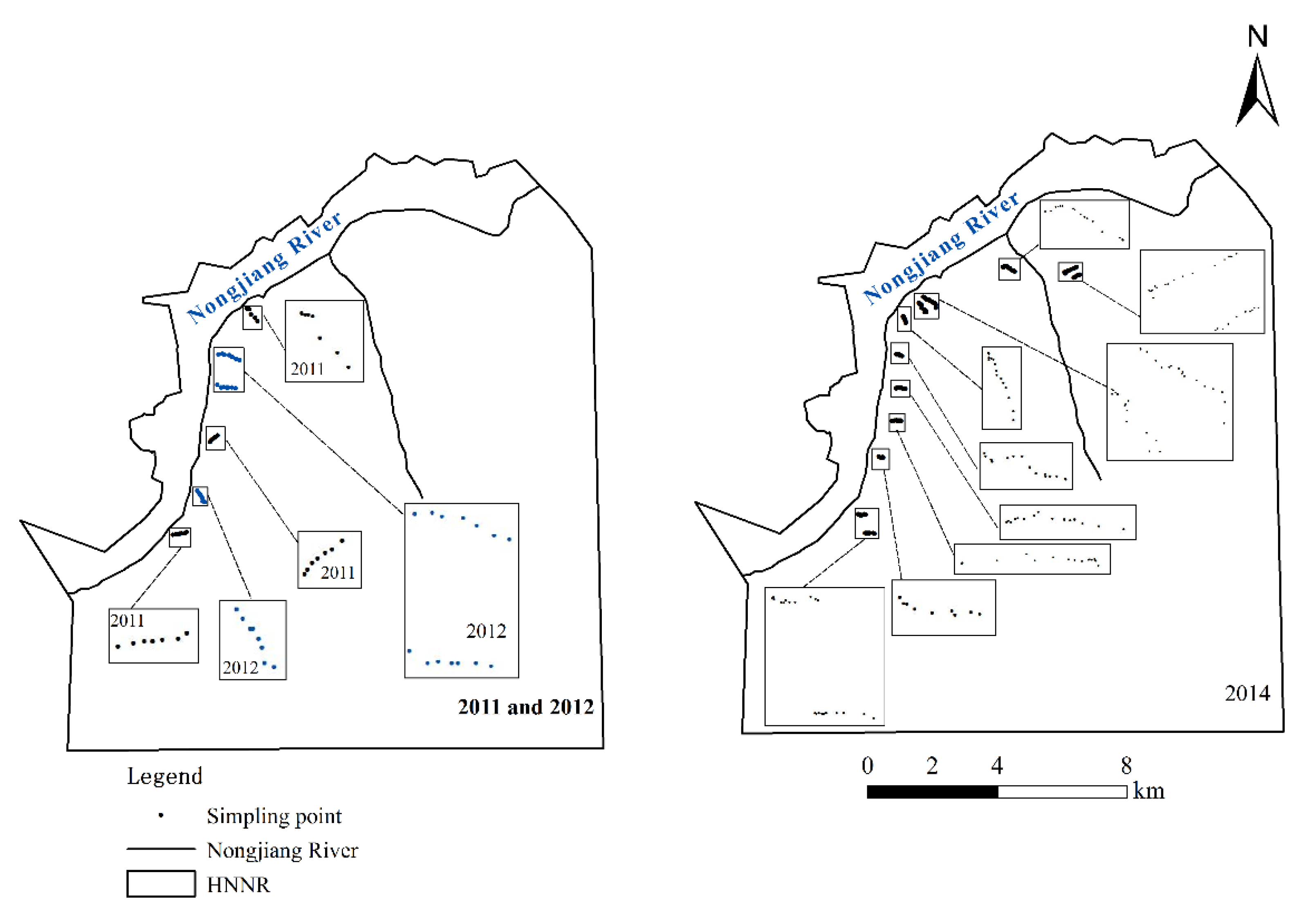
2.1. Study Area

Honghe National Nature Reserve (HNNR; 47°42′18″–47°52′07″ N and 133°34′38″–133°46′29″ E) is an alluvial plain in the Sanjiang Plain, located between Fujin and Tongjiang of Heilongjiang Province, with an area of 250.9 km2. HNNR was designated as a wetland of international importance by the Ramsar Wetland Convention Organization in 2002, and became one of 36 internationally important wetlands in China. The reserve is situated in the temperate humid climate region, with an annual mean temperature of around 1.9 °C, and an annual precipitation of approximately 585 mm, with 50–70% falling between July and September [34]. Two rivers enter the reserve. The Nongjiang River flows through the nature reserve near the northern boundary and the Wolan River originates from the central core area and flows into the Nongjiang River in the northern part of the reserve, both of which are primarily fed by rain water (Figure 1). Low-elevation areas are favorable for wetlands. Widespread inundation by floods is facilitated by a network of cross channels on low-terrain slopes (average slope is less than 1:10,000). Wetlands account for about 76.6% of the total area [35,36].
The vegetation types in the reserve include marsh vegetation, meadow vegetation, and forest vegetation. The zonation of vegetation, from wettest to driest, is characterized by the plant species Carex pseudocuraica, Carex lasiocarpa, Carex meyeriana, Calamagrostis angustifolia, Populus davidiana, and Betula platyphylla. In this study, the plant nomenclature is in accordance with Fu 1995 [37]. The distribution of vegetation zones frequently occurs along elevation gradients. One can find large variations in the water table depth from a wet meadow to meadow marsh and emergent marsh. Generally, permanently flooded emergent marshes (dominated by Carex pseudocuraica), seasonally flooded marshes (dominated by Carex lasiocarpa), and occasionally flooded marsh meadows (dominated by Calamagrostis angustifolia) are the key structural species in the vegetation of the typical hydrological gradient variation zone, though other species are also associated with this zone [11,29]. Swamp vegetation accounts for 50% of the protected area and is widely distributed in various low-lying areas and floodplains. The stable populations of Calamagrostis angustifolia, Carex lasiocarpa, and Carex pseudocuraica were employed as subjects.
As an internationally important wetland, this reserve has experienced heavy disturbance from regional agricultural development. In 1980, a canal was constructed in the west of HNNR, and the runoff of the Nongjiang River was cut off; the Nongjiang River was once an important surface water supply for HNNR. Therefore, the reserve suffered from a severe water shortage after the canal construction, which caused a continuous drop in surface water and groundwater. For all wetland vegetation types, marked decreases in the size of the area have been linked to a recorded lowering of the water level [38,39].

2.2. Methods

2.2.1. Sampling Method

Field data were collected by foot along transects of the study zone from May to September. With eighteen line transects (21 sample points (three line transects) in 2011, 21 sample points (three line transects) in 2012, and around six sample points along each transect and 168 sample points (12 line transects) in 2014), about fourteen sample points were included along each transect. A total of 210 sampling sites were thus produced (Figure 2). Each of the transect lines was designed along a moisture gradient from the stream bank to the floodplain terrace and passed through the plant communities perpendicular to the stream bank. Carex lasiocarpa showed distinct vegetation zonation, being typically situated along the streamside up to the Calamagrostis angustifolia community, which occupied higher floodplain terraces. At each sample point, three quadrats (50 × 50 cm2) were laid out randomly along transects and the plant species in each quadrat were collected with scissors. Records were made of the plants naturally growing in each of these quadrats. The geographical information of each sampling point was recorded using an E-survey E660 differential global positioning system (GPS). Based on the frequency of dominant wetland vegetation species under different hydrological gradients, the probability of wetland vegetation species appearing under different hydrological gradients was calculated. The dataset of 15 line transects was used for analysis in this study, and the field data of three line transects were used for validation (Figure 1 and Figure 2).

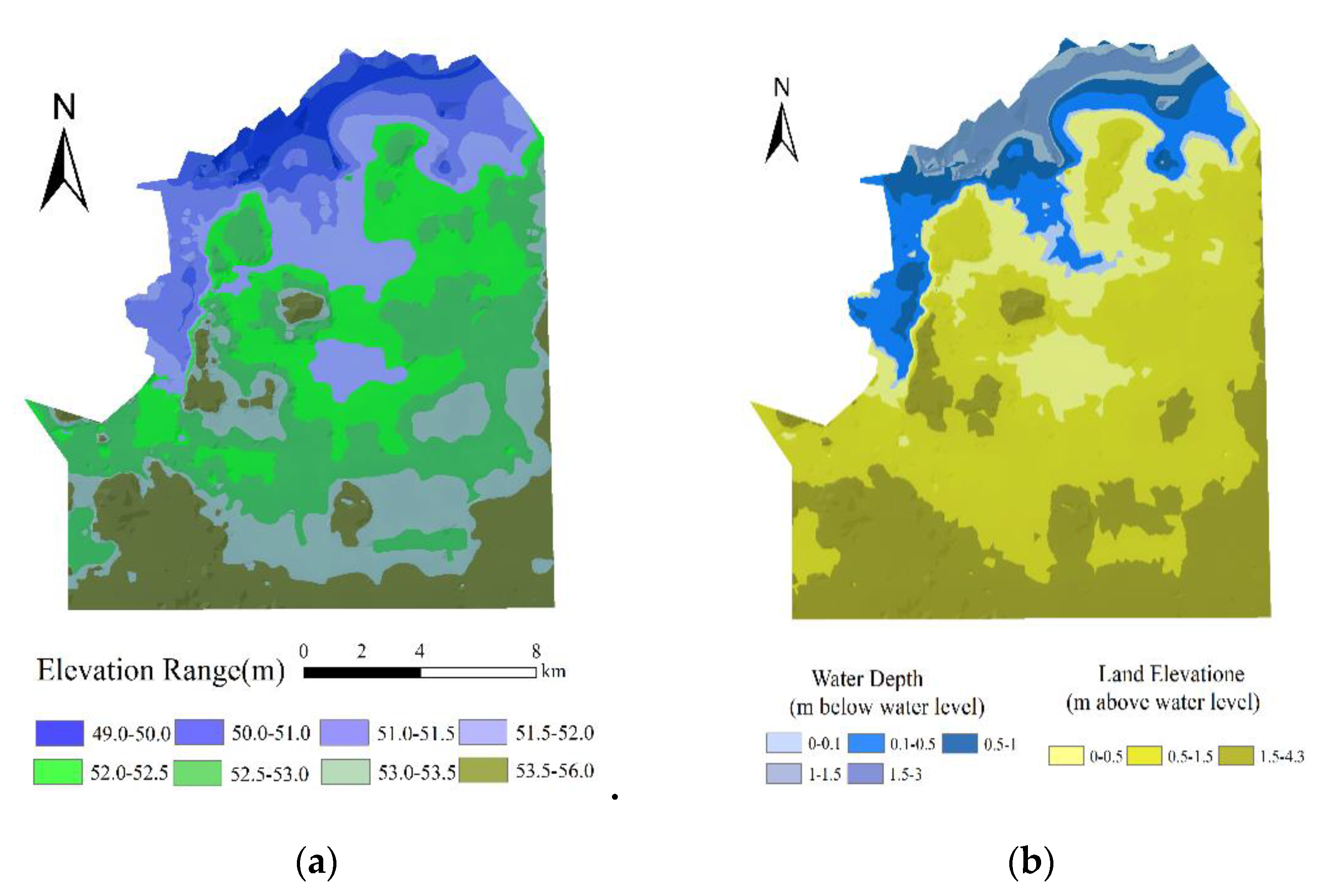
2.2.2. Hydrological Data

At each sampling point, the water depth needed to be measured using a meter stick. The soil moisture was measured by the Odyssey water level recording system from New Zealand, with a non-inundated area in wetlands. The water level of Nongjiang River in 2014 was obtained from a hydrological monitoring station.
The hydrological regime in wetlands is strongly correlated with the elevation of the ground surface and the water depth [40]. If the water level exceeds a certain elevation, the vegetation at this elevation is considered to be submerged. Therefore, the elevation and water depth were used to represent the water regime in the HNNR wetlands. An accurate water depth in the HNNR wetlands was acquired from a digital elevation model (DEM) of the study area, which was constructed by the 1:10,000 topographic map of the study area provided by the Heilongjiang Bureau of Surveying and Mapping Geoinformation. A DEM with a 5 m grid cell size was generated (Figure 3a). Water depth grids (and the elevation above water) (Figure 3b) were derived for each year of historical wetland data by subtracting the mean annual water level for that year from the DEM; average annual water levels were derived from monthly mean coordinated water levels.

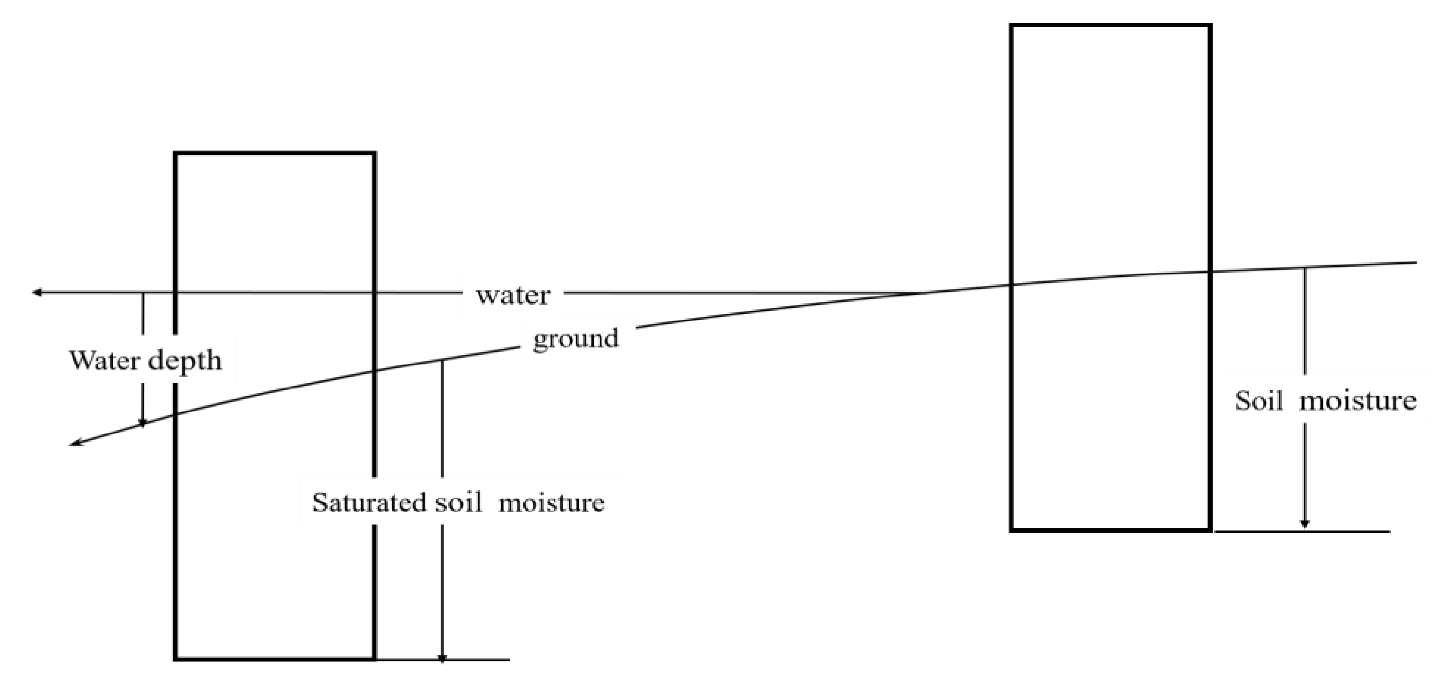
2.2.3. Conversion of the Hydrological Gradient

To compare the different hydrological regimes from inundated and non-inundated areas in wetlands (Figure 4), the value of the hydrological gradient was calculated according to the following equations.
W g 1 = S s × 1 + W l 100 × 1 2 ,
W g 2 = S m 100 × 1 2 ,
where Ss is the saturated soil moisture (%); Wl is the water level (cm); Sm is the soil moisture (%); Wg1 is the inundated area; Wg2 is the non-inundated area; and Wg1 and Wg2 are dimensionless units. Taking the water surface as the benchmark, the data are derived from a section corresponding to 1 cubic meter above and below this surface.
For the non-inundated area, hydrological gradients (Wg2) were calculated by using the actual soil water content measured(Sm) during field sampling. The hydrological gradient for the inundated area was calculated by using the saturated soil moisture (Ss) and water level (Wl). The saturated soil moisture (Ss) corresponding to different vegetation was different, where the average value of the soil saturated water content for the community of Calamagrostis angustifolia was 60%, that of Carex lasiocarpa was 80%, and that of Carex pseudocuraica was 90%, according to the measured values of the saturated soil moisture (Figure 4).

2.2.4. Gaussian Logistic Regression Model

The Gaussian model was adopted to describe the relationship between plant species and the environment [22,41]. Studies on the response of the reed to the water depth based on the Gaussian model have achieved good results [42,43]. The Gaussian model equation is as follows:
y = c   exp [ 1 2 ( x u ) 2 / t 2 ] ,
where y represents an indicator of the biological characteristics of plant species, including the abundance, density, biomass, probability of occurrence, etc.; x is the value of environmental factors; c is the maximum value of y; u is the optimum ecological amplitude of the species to environmental factors; and t represents the tolerance of the plant species and is an indicator used to describe the ecological range of the species. Generally, the optimum ecological amplitude of species to environmental factors changes within the 2t range. In this study, First Optimization (1stOpt) software was used for curve fitting. The term y represents the probability of occurrence of wetland vegetation, and x represents the hydrological gradient of the wetland.

2.2.5. Nonlinear Regression and Correlation Test

Nonlinear regression by the F test was used to analyze the relationship between the probability of occurrence and the hydrological gradient. A correlation test by the T test was applied to test the correlation between the probability of occurrence and the hydrological gradient and simulated and observed results. All of the statistical methods were carried out in First Optimization 1.5 and Origin2018 software (data available upon request).

3. Results

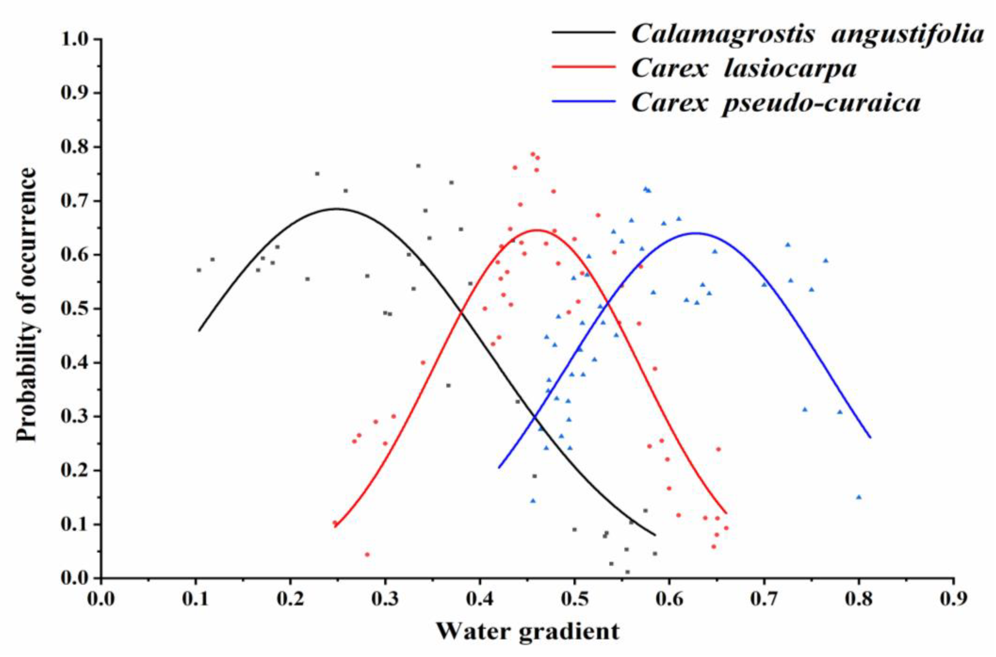
3.1. Species Response to the Hydrological Gradient

3.1.1. Response of Calamagrostis angustifolia to the Hydrological Gradient

A total of 34 Calamagrostis angustifolia community sampling datasets (spots without Calamagrostis angustifolia removed) were statistically analyzed. The probability of occurrence of Calamagrostis angustifolia was strongly correlated to the hydrological gradient (Table 1). The probability of occurrence and hydrological gradient were fit using First Optimization (1stOpt) software, and the empirical model for the probability of occurrence and hydrological gradient were obtained. The obtained curve was fit with the Gaussian model (Figure 5). Using regression analyses, the Gaussian regression equation and regression curve were obtained, and can be expressed as the following equation:
y = 0.69 exp [ 1 2 ( x 0.25 ) 2 / ( 0.16 ) 2 ] .
The optimum ecological amplitude of Calamagrostis angustifolia to the hydrological gradient based on the probability of occurrence was [0.09, 0.41] and the optimum growing point was 0.25.

3.1.2. Response of Carex lasiocarpa to the Hydrological Gradient

A total of 51 Carex lasiocarpa community sampling datasets (spots without Carex lasiocarpa removed) were statistically analyzed. The probability of occurrence of Carex lasiocarpa was strongly correlated to the hydrological gradient (Table 1). The probability of occurrence and hydrological gradient were fit by First Optimization (1stOpt) software, and the empirical model for the probability of occurrence and hydrological gradient was obtained. The obtained curve was fit with the Gaussian model (Figure 5). Employing regression analyses, the Gaussian regression equation and regression curve were obtained, and can be expressed using the following equation:
y = 0.65 exp [ 1 2 ( x 0.46 ) 2 / ( 0.11 ) 2 ] .
The optimum ecological amplitude of Carex lasiocarpa to the hydrological gradient based on the probability of occurrence was [0.35, 0.57] and the optimum growing point was 0.46.

3.1.3. Response of Carex pseudocuraica to the Hydrological Gradient

A total of 46 Carex pseudocuraica community sampling datasets (spots without Carex pseudocuraica removed) were statistically analyzed. The probability of occurrence for Carex pseudocuraica was strongly correlated to the hydrological gradient (Table 1). The probability of occurrence and hydrological gradient were fit by First Optimization (1stOpt) software, and the empirical model for the probability of occurrence and hydrological gradient was obtained. The obtained curve was fit with the Gaussian model (Figure 5). Employing regression analyses, the Gaussian regression equation and regression curve were obtained, and can be expressed as the following equation:
y = 0.64 exp [ 1 2 ( x 0.63 ) 2 / ( 0.14 ) 2 ] .
The optimum ecological amplitude of Carex pseudocuraica to the hydrological gradient based on the probability of occurrence was [0.49, 0.77] and the optimum growing point was 0.63.

3.2. Comparison of Probabilities of Occurrence Responses to the Hydrological Gradient

The change of hydrological gradient had a significant impact on the probability of occurrence for three typical types of wetland vegetation (Figure 5). The probability of occurrence for the three typical types of wetland vegetation increased first and then declined with the change in hydrological conditions, showing a single peak curve. This probably followed a distinct order of Calamagrostis angustifolia, Carex lasiocarpa, and Carex pseudocuraica with the hydrological gradient going from small to large. The distribution range of Calamagrostis angustifolia was from no water surface area to 0.63, that of Carex lasiocarpa was from 0.25 to 0.63, and that of Carex pseudocuraica was from 0.40 to 0.80. In the study area, without a water surface (i.e., the hydrological gradient was less than 0.15), only the community of Calamagrostis angustifolia appeared; when the hydrological gradient was 0.25, the community of Carex lasiocarpa began to appear until the hydrological gradient was greater than 0.66; and when the hydrological gradient was 0.40, the community of Carex pseudocuraica began to appear.

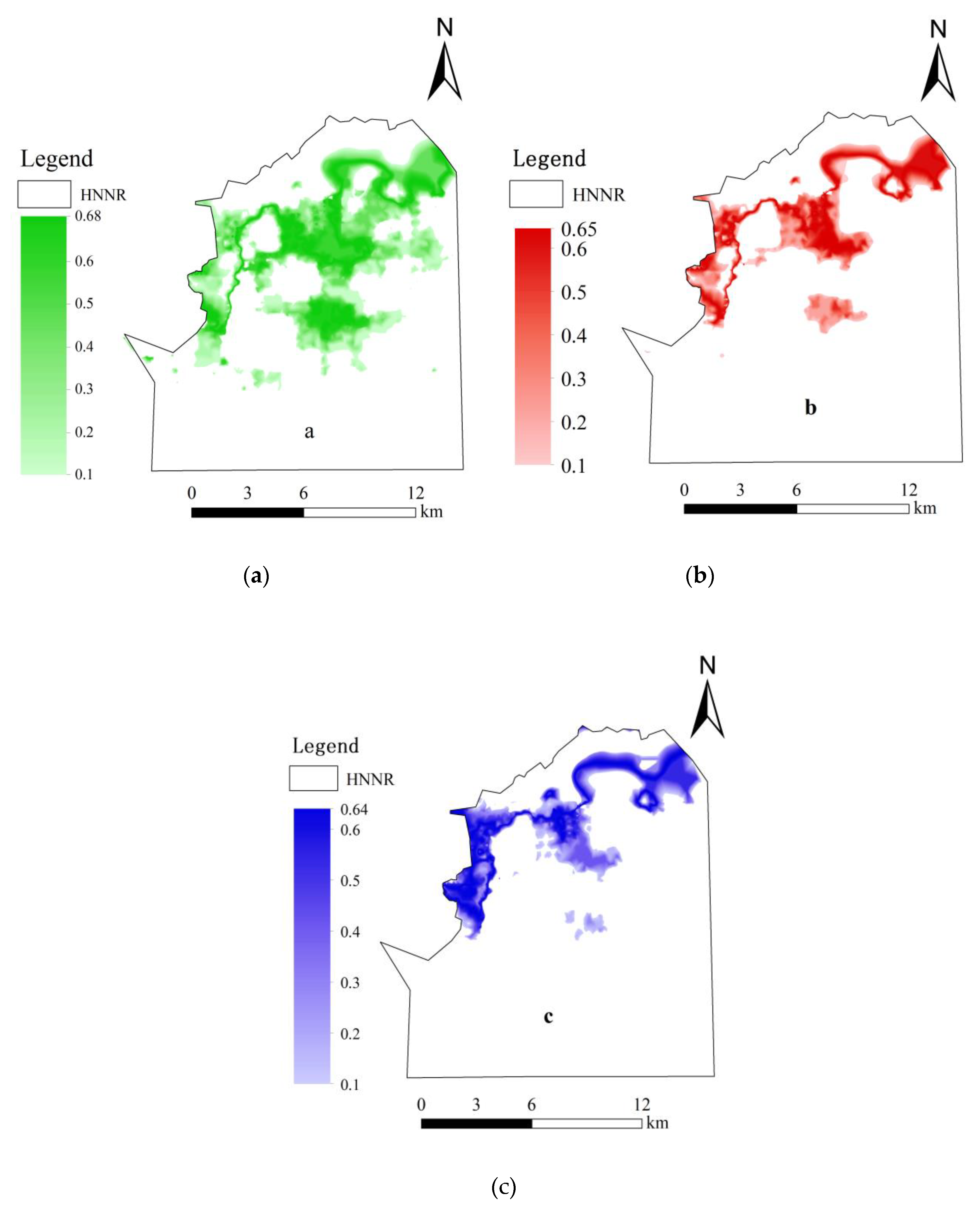
3.3. Simulation of the Spatial Distribution Probability

Using the relationship between the three wetland plant species and the hydrological gradient, the spatial pattern of wetland vegetation communities under different hydrological gradients was simulated and predicted across the whole study area using the spatial analysis tools of Arcgis10.5. The results of the probability of occurrence model, when integrated with GIS techniques, provide a means to predict and characterize the spatial distribution probability of the three types of wetland vegetation under different hydrological gradients. The spatial distribution of three typical dominant plants in grid format with a spatial resolution of 5 m was generated from our established model (Figure 6). The maps show that with an increase in distance to the water body, the probability of occurrence increased gradually for Calamagrostis angustifolia and decreased gradually for Carex pseudocuraica. Additionally, there was a high probability of occurrence of Carex pseudocuraica close to the water body. Moreover, a high probability of occurrence for Carex lasiocarpa was found between areas dominated by Carex pseudocuraica and Calamagrostis angustifolia. The three typical dominant plant communities displayed distinct vegetation zonation along a hydrological gradient in elevation, from the stream bank to the floodplain terrace.
The vegetation types and distribution areas of wetlands in the future could be predicted. The result of the spatial distribution probability reflected the community pattern (area and distribution) of wetland vegetation. It can be seen that the distribution area of Calamagrostis angustifolia was 77.30 km2, the distribution area of Carex lasiocarpa was 40.40 km2, and the distribution area of Carex pseudocuraica was 39.50 km2 (Figure 6).

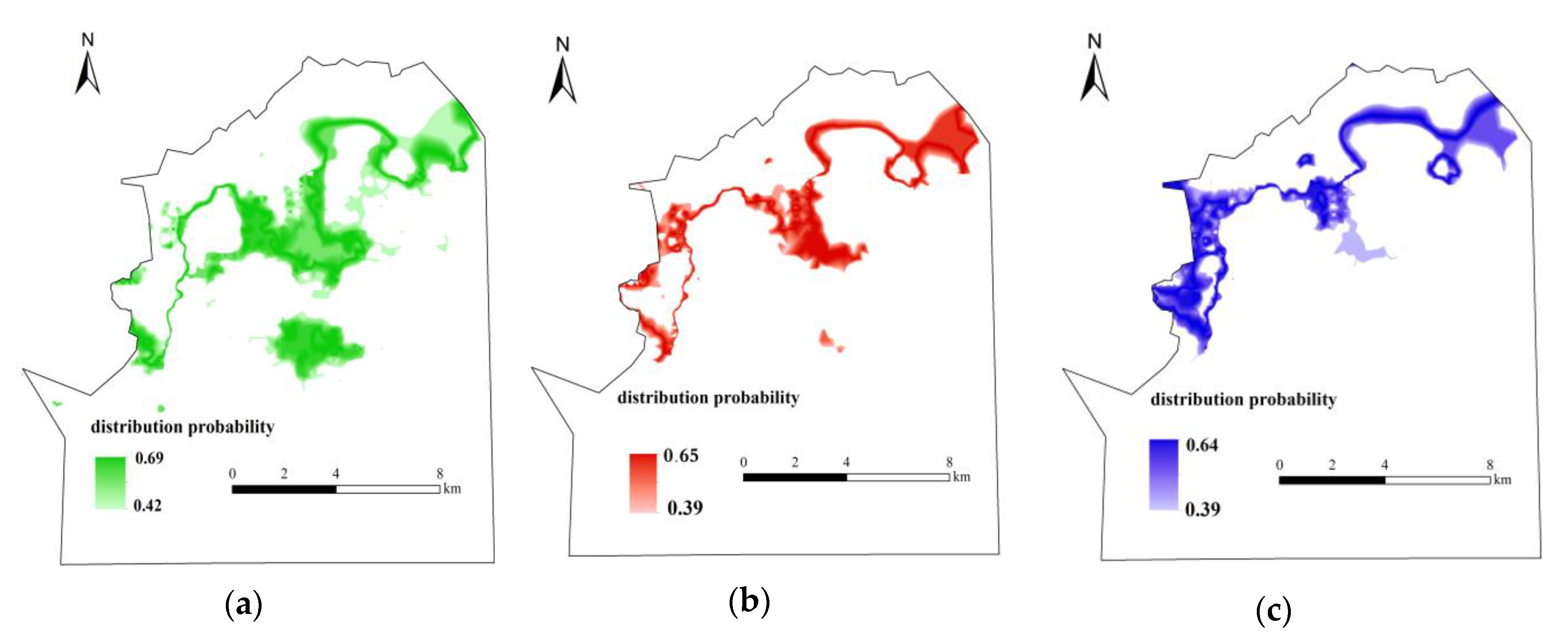
3.4. The Distribution of the Most Suitable Habitat

The corresponding spatial distribution probability interval of vegetation was obtained according to the optimum ecological amplitude of wetland vegetation and the hydrological gradient based on the results of the probability of occurrence model. The distribution probability interval of Calamagrostis angustifolia was [0.42, 0.69], the distribution probability interval of Carex lasiocarpa was [0.39, 0.65], and the distribution probability interval of Carex pseudocuraica was [0.39, 0.64]. Finally, the distribution map of the most suitable habitat for each type of vegetation was developed (Figure 7).
Calamagrostis angustifolia grows in seasonally flooded areas where the hydrological gradient drops; Carex lasiocarpa is distributed in the transition zone between the marsh vegetation and the seasonally flooded vegetation; and Carex pseudocuraica exists near the river where the hydrological gradient is relatively large.

3.5. Validation Results

For this study, three line transects (transects1, 2, and 3 in Figure 1) were randomly selected to validate the simulation results of the model. The observation and simulation results of the vegetation distribution probability are presented as a tendency chart shown in Figure 8 (only transect 2). A comparison of the observed and simulated vegetation distribution probability shows good agreement, indicating that the model shows good representation of the vegetation distribution probability in the Honghe wetland. Furthermore, the performance evaluation criteria were also calculated for the vegetation distribution probability. Table 2 outlines the R2, standard error (SE) and standard error of the mean (SEM) values for the simulation results. The R2, SE and SEM values of Calamagrostis angustifolia were 0.62, 0.24, 0.11 and those of Carex lasiocarpa were 0.68, 0.27 and 0.17 for transect 1. The R2, SE and SEM values of Calamagrostis angustifolia were 0.84, 0.14 and 0.13. The values for Carex lasiocarpa were 0.93, 0.10 and 0.02, and for Carex pseudocuraica the values were 0.97, 0.09 and 0.02 for transect 2. For transect 3, the R2, SE, and SEM values were 0.71, 0.19 and 0.07 for Carex lasiocarpa and 0.79, 0.22 and 0.09 for Carex pseudocuraica.Allvalues were above 0.5, suggesting satisfactory model performance.
There were a few differences between the observed and simulated vegetation distribution probabilities in transects 1 and 3 (Table 2). The major discrepancies between the simulated and observed distribution probability were found for Carex pseudocuraica in transect 1 and Calamagrostis angustifolia in transect 3.
We obtained the simulation tendency charts for transect 2; they are presented in Figure 8. The results show that the observed and simulated distribution probability values follow the hydrological gradient of the studied areas. The method was validated in accordance with the line transects corresponding to sampling points from the island to the river, that is, from a low to high hydrological gradient. As shown by the simulation values and observation values in Figure 8, an increase in the hydrological gradient results in a higher distribution probability for Calamagrostis angustifolia initially, followed by Carex lasiocarpa and finally, Carex pseudocuraica. This further verifies the applicability of the simulation results and reveals the response of the vegetation distribution to the hydrological gradient in the Honghe wetland.

4. Discussion

4.1. Modeling the Spatial Distribution of Wetland Vegetation Species’ Response to the Hydrological Gradient

Hydrological conditions have been demonstrated to be the main factor controlling changes in vegetation community composition in the Sanjiang Plain [11,34,44]. How the probability of occurrence varies between different plant species in response to an increasing hydrological gradient may play an important role in the distribution of vegetation zones in these freshwater marshes. At present, most research in this study area is still mostly focused on distribution responses of individual species to the water depth in the Sanjiang Plain [26,27], while little attention has been paid to research on the vegetation zonation pattern distribution along hydrological gradients in wetlands, especially the ecological spatial distribution pattern and the process of quantitative research across a larger landscape.It is highly relevant to combine large numbers of observations with species response models to predict future vegetation changes dependent on water level changes. Therefore, based on the GIS and results of the probability of occurrence model, the distribution probability of wetland vegetation under the hydrological gradient was predicted, and further, the dominant species under the hydrological gradient were predicted. Considering both the change in the hydrological regime of the HNNR and the spatial probability distribution of dominant species, the future patterns of vegetation types and distribution areas of the wetland can be predicted (Figure 6 and Figure 7). Our results show that the dominant wetland vegetation species had its own optimum ecological amplitude (Figure 4); there were substantial optimum ecological amplitude overlaps, but a clear differentiation of optima among the studied species. This may indicate that the spatial distribution of these species is driven, in part, by a changing hydrological gradient. This finding is consistent with previous research [11,28]. In the process of conducting the vegetation survey in the study area, it was found that dominant species and associated species coexist in most cases and Carex lasiocarpa acts as a transitional zone, representing the transition from a low-water-gradient Calamagrostis angustifolia community to a high-water-gradient Carex pseudocuraica community. The simulation results are consistent with the actual sampling, which verifies the rationality of the simulation results and reveals the horizontal zonal law of typical wetland vegetation in HNNR.
A water level decrease was the factor most clearly related to the changes along the marsh zonation. The temperature showed an increasing trend, while precipitation fluctuated without a trend; this would result in a decline in humidity [44]. These findings indicate that if the drying of wetlands in this region continues, then Carex lasiocarpa and Carex pseudocuraica marshes will gradually be replaced by Calamagrostis angustifolia wet meadows in the near future. This will result in a reduction in biodiversity. Our results can be applied in conservation management. For example, knowledge about the water depth optimum ecological amplitude of wetland plants is a prerequisite for hydrological restoration. This can be valuable for understanding the vulnerability of wetland ecosystems and informing resource management decisions in the Sanjiang Plain, Northeast China.

4.2. Uncertaintyof the Modeling the Spatial Distribution of Wetland Vegetation Species’ Response to the Hydrological Gradient

We found that in the validation results, there were major discrepancies between the simulated and observed probability of occurrence for Carex pseudocuraica in transect 1 andCalamagrostis angustifolia in transect 3 (Table 2). In field sampling, Carex pseudocuraica was found in the deepest parts of the Honghe wetland, which are particularly inaccessible and are difficult places to work. Therefore, there was no observed value for this area, only a simulated value, resulting in a poor simulation effect. The final simulation results in the study area were based on a DEM of the study area for obtaining the hydrological gradient, from which the distribution probability under hydrological gradient change can be derived. Therefore, the simulation results were directly related to the accuracy of topography and the DEM. Meanwhile, long-term field sampling datasets and high-resolution remote sensing images must be considered and should be a focus of attention in future studies on simulations of vegetation responses to hydrology in floodplain wetlands. In addition to this, species interactions (correlations with other environmental factors, e.g., competition and soil nutrients) can also influence the pattern of simulation [2,4,11,45]. Although our results show that the flooding depth works reasonably well as a predictor in modeling, the nutrient availability should be included in future studies on the ecological response of wetland plant species, since the soil properties together with draining can also determine the species distribution in the Sanjiang wetlands. Therefore, there are many dominant factors that affect the spatial distribution of vegetation in other study areas. The establishment of the model should comprehensively consider the influence of dominant factors.

5. Conclusions

This study investigated three wetland vegetation community distribution responses to the hydrological gradient in the Sanjiang Plain, Northeast China. The main results of this study are as follows: (1) ecological response curves were generated, and the optimum ecological amplitude was modeled based on the probability of occurrence; (2) the wetland vegetation spatial distribution in response to changes in the hydrological gradient was simulated across a larger landscape and the most suitable habitats were determined; (3) the model simulation results were verified, showing that this approach was able to simulate the spatial distribution pattern of the wetland vegetation community in the Sanjiang Plain, Northeast China.

Author Contributions

D.Y. and Z.L. contributed to come up with the initial ideas and wrote the main manuscript text; D.X. reviewed and edited the manuscript; Y.X. and D.S. prepared figures and tables and related analyses; D.Y. discussed the results and wrote the paper; all authors made revisions and improvements to the final version. All authors have read and agreed to the published version of the manuscript.

Funding

The study of this paper was supported by National Natural Science Foundation of China (project no. 41471078, 41871097), Jiangsu Agricultural Science and Technology Innovation Fund (project no. CX (18)2026), Jiangsu 333 Talent Program, Research Foundation for Advanced Talents of Nanjing Forestry University, and the Priority Academic Program Development of Jiangsu Higher Education Institution(PAPD).

Acknowledgments

The authors gratefully acknowledge editors and reviewers for raising suggestions and comments on this paper.

Conflicts of Interest

The authors declare no conflict of interest.

References

  1. Foti, R.; Del Jesus, M.; Rinaldo, A.; Rodriguez-Iturbe, I. Hydroperiod regime controls the organization of plant species in wetlands. Proc. Natl. Acad. Sci. USA 2012, 109, 19596–19600. [Google Scholar] [CrossRef] [PubMed] [Green Version]
  2. Kinser, P.; Fox, S.; Keenan, L.; Ceric, A.; Baird, F. Hydrology and the Distribution of Floodplain Plant Communities of the Upper Set. Johns River, Florida—Using Transects to Track the Movement of Plant Communities Along a Changing Hydrological Gradient; St. Johns River Water Management District: Parateca, FL, USA, 2012. [Google Scholar]
  3. Todd, M.J.; Muneepeerakul, R.; Pumo, D.; Azaele, S.; Miralles-Wilhelm, F.; Rinaldo, A.; Rodriguez-Iturbe, I. Hydrological drivers of wetland vegetation community distribution within Everglades National Park, Florida. Adv. Water Resour. 2010, 33, 1279–1289. [Google Scholar] [CrossRef]
  4. Wilcox, D.A.; Xie, Y.C. Predicting wetland plant community responses to proposed water-level-regulation plans for lake ontario: GIS-based modeling. J. Great Lakes Res. 2007, 33, 751–773. [Google Scholar] [CrossRef]
  5. Geest, G.J.V.; Coops, H.; Roijackers, R.M.M.; Buijse, A.D.; Scheffer, M. Succession of aquatic vegetation driven by reduced water-level fluctuations in floodplain lakes. J. Appl. Ecol. 2005, 42, 251–260. [Google Scholar] [CrossRef]
  6. Havens, K.E. Submerged aquatic vegetation correlations with depth and light attenuating materials in a shallow subtropical lake. Hydrobiologia 2003, 493, 173–186. [Google Scholar] [CrossRef]
  7. Casanova, M.T.; Brock, M.A. How do depth, duration and frequency of flooding influence the establishment of wetland plant communities? Plant Ecol. 2000, 147, 237–250. [Google Scholar] [CrossRef]
  8. Wang, H.Y.; Chen, J.K.; Zhou, J. Influence of water level gradiention plant growth, reproduction and biomass allocation of wetland plant species. Chin. J. Plant Ecol. 1999, 3, 269–274. (In Chinese) [Google Scholar]
  9. Magee, T.K.; Kentula, M.E. Response of wetland plant species to hydrologic conditions. Wetl Ecol. Manag. 2005, 13, 163–181. [Google Scholar] [CrossRef]
  10. Wang, Q.L.; Chen, J.R.; Liu, H.; Yi, L.Y.; Li, W.; Liu, F. The growth responses of two emergent plants to the water depth. Acta Hydro. Sin. 2012, 33, 583–587. (In Chinese) [Google Scholar]
  11. Lou, Y.J.; Wang, G.P.; Lu, X.G.; Jiang, M.; Zhao, K.Y. Zonation of plant cover and environmental factors in wetlands of the Sanjiang Plain, northeast China. Nord. J. Bot. 2013, 31, 748–756. [Google Scholar] [CrossRef]
  12. Engels, J.G.; Jensen, K. Patterns of wetland plant diversity along estuarine stress gradients of the Elbe (Germany) and Connecticut (USA) Rivers. Plant Ecol.Diver. 2009, 2, 301–311. [Google Scholar] [CrossRef]
  13. Zhou, D.; Gong, H.; Luan, Z.; Hu, J.; Wu, F. Spatial pattern of water controlled wetland communities on the Sanjiang Floodplain, Northeast China. Community Ecol. 2006, 7, 223–234. [Google Scholar] [CrossRef]
  14. Wilson, S.D.; Keddy, P.A. Plant Zonation on a Shoreline Gradient: Physiological Response Curves of Component Species. J. Ecol. 1985, 73, 851–860. [Google Scholar] [CrossRef]
  15. Shi, F.X.; Song, C.C.; Zhang, X.H.; Mao, R.; Guo, Y.D.; Gao, F.Y. Plant zonation patterns reflected by the differences in plant growth, biomass partitioning and root traits along a water level gradient among four common vascular plants in freshwater marshes of the Sanjiang Plain, Northeast China. Ecol. Eng. 2015, 81, 158–164. [Google Scholar] [CrossRef]
  16. Correa-Araneda, F.J.; Urrutia, J.; Soto-Mora, Y.; Figueroa, R.; Hauenstein, E. Effects of the hydroperiod on the vegetative and community structure of freshwater forested wetlands, Chile. J.Freshw. Ecol. 2012, 27, 459–470. [Google Scholar] [CrossRef] [Green Version]
  17. Xie, Y.H.; Ren, B.; Li, F. Increased nutrient supply facilitates acclimation to high-water level in the marsh plant Deyeuxia angustifolia: The response of root morphology. Aquat. Bot. 2009, 91, 1–5. [Google Scholar] [CrossRef]
  18. Crain, C.M. Interactions between marsh plant species vary in direction and strength depending on environmental and consumer context. J. Ecol. 2008, 96, 166–173. [Google Scholar] [CrossRef]
  19. Seabloom, E.W.; Van der Valk, A.G.; Moloney, K.A. The role of water depth and soil temperature in determining initial composition of prairie wetland coenoclines. Plant. Ecol. 1998, 138, 203–216. [Google Scholar] [CrossRef]
  20. Dwire, K.A.; Kauffman, J.B.; Baham, B.J.E. Plant biomass and species composition along an environmental gradient in montane riparian meadows. Oecologia 2004, 139, 309–317. [Google Scholar] [CrossRef]
  21. Violle, C.; Bonis, A.; Plantegenest, M.; Cudennec, C.; Damgaard, C.; Marion, B.; Le Coeur, D.; Bouzille, J.B. Plant functional traits capture species richness variations along a flooding gradient. Oikos 2011, 120, 389–398. [Google Scholar] [CrossRef]
  22. Coudun, C.; Gegout, J.C. The derivation of species response curves with gaussian logistic regression is sensitive to sampling intensity and curve characteristics. Ecol. Model. 2006, 199, 164–175. [Google Scholar] [CrossRef]
  23. Lee, K.H.; Lunetta, R.S. Wetland detection methods. In Wetland and Environmental Application of GIS; Lyon, J.G., McCarthy, J., Eds.; Lewis: New York, NY, USA, 1995; pp. 249–284. [Google Scholar]
  24. Trepel, M.; Dall'O', M.; Cin, L.D.; Wit, M.D.; Opitz, S.; Palmeri, L.; Persson, J.; Pieterse, N.; Timmermann, T.; Bendoricchio, G.; et al. Models for wetland planning, design and management. EcoSys Bd. 2000, 8, 93–137. [Google Scholar]
  25. Hebb, A.J.; Mortsch, L.D.; Deadman, P.J.; Cabrera, A.R. Modeling wetland vegetation community response to water-level change at Long Point, Ontario. J. Great Lakes Res. 2013, 39, 191–200. [Google Scholar] [CrossRef]
  26. Jiao, C.C.; Zhou, D.M. Modeling the spatial distribution of Carex pseudocuraica in a freshwater marsh, Northeast China. Wetlands 2014, 34, 267–276. [Google Scholar] [CrossRef]
  27. Luan, Z.Q.; Wang, Z.X.; Yan, D.D.; Liu, G.H.; Xu, Y.Y. The ecological response of Carex lasiocarpa community in the Riparian Wetlands to the environmental gradient of water depth in Sanjiang Plain, Northeast China. Sci. World J. 2013, 2013, 1–7. [Google Scholar]
  28. Lou, Y.J.; Gao, C.Y.; Pan, Y.W.; Xue, Z.S.; Liu, Y.; Tang, Z.H.; Jiang, M.; Lu, X.G.; Rydin, H. Niche modelling of marsh plants based on occurrence and abundance data. Sci. TotalEnviron. 2018, 616, 198–207. [Google Scholar] [CrossRef] [PubMed]
  29. Lou, Y.J.; Pan, Y.W.; Gao, C.Y.; Jiang, M.; Lu, X.G.; Xu, Y.J. Response of plant height, species richness and aboveground biomass to flooding gradient along vegetation zones in floodplain wetlands, Northeast China. PLoS ONE 2016, 11, e0153972. [Google Scholar]
  30. Adam, E.; Mutanga, O.; Rugege, D. Multispectral and hyperspectral remote sensing for identification and mapping of wetland vegetation: A review. Wetl. Ecol. Manag. 2010, 18, 281–296. [Google Scholar] [CrossRef]
  31. Zhao, K.Y. Mires in China; Science Press: Beijing, China, 1999. (In Chinese) [Google Scholar]
  32. Luo, W.B.; Song, F.B.; Xie, Y.H. Trade-off between tolerance to drought and tolerance to flooding in three wetland plants. Wetlands 2008, 28, 866–873. [Google Scholar] [CrossRef]
  33. Zhang, X.H.; Mao, R.; Gong, C.; Yang, G.S.; Lu, Y.Z. Effects of hydrology and competition on plant growth in a freshwater marsh of northeast China. J. Freshwater. Ecol. 2014, 29, 117–127. [Google Scholar] [CrossRef] [Green Version]
  34. Luan, Z.Q.; Deng, W.; Zhu, B.G. Estimation of eco-environmental water consumption for Honghe national nature reserve wetlands. Arid Land Resour. Environ. 2004, 18, 59–63. [Google Scholar]
  35. Liu, X.T. Natural Environmental Changes and Ecological Protection in the Sanjiang Plain; Science Press: Beijing, China, 2002. (In Chinese) [Google Scholar]
  36. Zhou, D.M.; Gong, H.L. Hydro-Ecological Modeling of the Honghe National Natural Reserve; China Environmental Science Press: Beijing, China, 2007. (In Chinese) [Google Scholar]
  37. Fu, P.Y. Clavis Plantarum Chinese Boreali-Orientalis; Science Press: Beijing, China, 1995. (In Chinese) [Google Scholar]
  38. Zhou, D.M.; Gong, H.L.; Wang, Y.Y.; Khan, S.B.; Zhao, K.Y. Driving forces for the marsh wetland degradation in the Honghe National Nature Reserve in Sanjiang plain, Northeast China. Environ. Model. Assess. 2009, 14, 101–111. [Google Scholar] [CrossRef]
  39. Wan, L.H.; Zhang, Y.W.; Zhang, X.Y.; Qi, S.Q.; Na, X.D. Comparison of land use/land cover change and landscape patterns in Honghe National Nature Reserve and the surrounding Jiansanjiang Region, China. Ecol. Indic. 2015, 51, 205–214. [Google Scholar] [CrossRef]
  40. Urban, K.E. Oscillating vegetation dynamics in a wet heathland. J. Veg.Sci. 2009, 16, 111–120. [Google Scholar] [CrossRef]
  41. Zhang, J.T. Quantitative Ecology; Science Press: Beijing, China, 2010. (In Chinese) [Google Scholar]
  42. Cui, B.S.; Zhao, X.S.; Yang, Z.F.; Tang, N.; Tan, X.J. The response of reed community to the environment gradient of water depth in the Yellow River Delta. Acta. Ecol. Sin. 2006, 3, 194–202. [Google Scholar] [CrossRef]
  43. Bi, Z.L.; Xiong, X.; Lu, F.; He, Q.; Zhao, X.S. Studies on ecological amplitude of reed to the environmental gradient of waterdepth. Shandong For. Sci.Technol. 2007, 4, 1–3. (In Chinese) [Google Scholar]
  44. Lou, Y.J.; Zhao, K.Y.; Wang, G.P.; Jiang, M.; Lu, X.G.; Rydin, H. Long term changes in marsh vegetation in Sanjiang plain, Northeast China. J. Veg. Sci. 2015, 26, 643–650. [Google Scholar] [CrossRef]
  45. Austin, M.P. Spatial prediction of species distribution: An interface between ecological theory and statistical modelling. Ecol. Model. 2002, 157, 101–118. [Google Scholar] [CrossRef] [Green Version]
Figure 1. Location of the study area and distribution map of field sampling sites in the Honghe National Nature Reserve (HNNR).
Water 12 02041 g001
Figure 2. Location of the sampling spots.
Water 12 02041 g002
Figure 3. (a) Topographical elevation (m) and (b) elevation relative to the water level.
Water 12 02041 g003
Figure 4. Conversion of the hydrological gradient.
Water 12 02041 g004
Figure 5. Species response curves for the hydrological gradient based on the probability of occurrence indicated by the Gaussian model for wetland vegetation.
Water 12 02041 g005
Figure 6. Spatial distribution probability maps of wetland vegetation (a): Calamagrostis angustifolia; (b): Carex lasiocarpa; (c): Carex pseudocuraica.
Water 12 02041 g006
Figure 7. The distribution map of the most suitable habitat for wetland vegetation (a): Calamagrostis angustifolia; (b): Carex lasiocarpa; (c): Carex pseudocuraica.
Water 12 02041 g007
Figure 8. Comparison of observed and simulated vegetation probability of occurrence in transect 2: (a): Calamagrostis angustifolia; (b): Carex lasiocarpa; (c): Carexpseudocuraica.
Water 12 02041 g008
Table 1. The coefficient obtained from the Gaussian regression model for each species, together with the error indices.
Wetland Vegetation SpeciesCoefficientPerformance Evaluation Criteria (p < 0.05)
cutF-StatisticRR2RMSESSE
Calamagrostis angustifolia0.680.250.16140.40.900.810.110.40
Carex lasiocarpa0.650.460.11241.90.910.830.090.41
Carex pseudocuraica0.620.630.1459.880.760.580.100.42
Abbreviations: root-mean-square error(RMSE); sum of squares for error (SSE).
Table 2. Statistical comparison of the observed and simulated vegetation distribution probability in the HNNR. Abbreviations: standard error (SE); standard error of the mean (SEM).
TransectWetland Vegetation SpeciesPerformance Evaluation Criteria (p < 0.05)
R2SESEM
Transect 1 Calamagrostis angustifolia0.620.240.11
Carex lasiocarpa0.680.270.17
Carex pseudocuraica
Transect 2Calamagrostis angustifolia0.840.140.03
Carex lasiocarpa0.930.100.02
Carex pseudocuraica0.970.090.02
Transect 3Calamagrostis angustifolia
Carex lasiocarpa0.710.190.07
Carex pseudocuraica0.790.220.09

