Impacts of Tide Gate Modulation on Ammonia Transport in a Semi-closed Estuary during the Dry Season—A Case Study at the Lianjiang River in South China


Abstract
:1. Introduction
2. Materials and Methods
2.1. Study Site
2.2. Numerical Model
2.3. Model Setting
2.4. Analysis Methods
3. Results
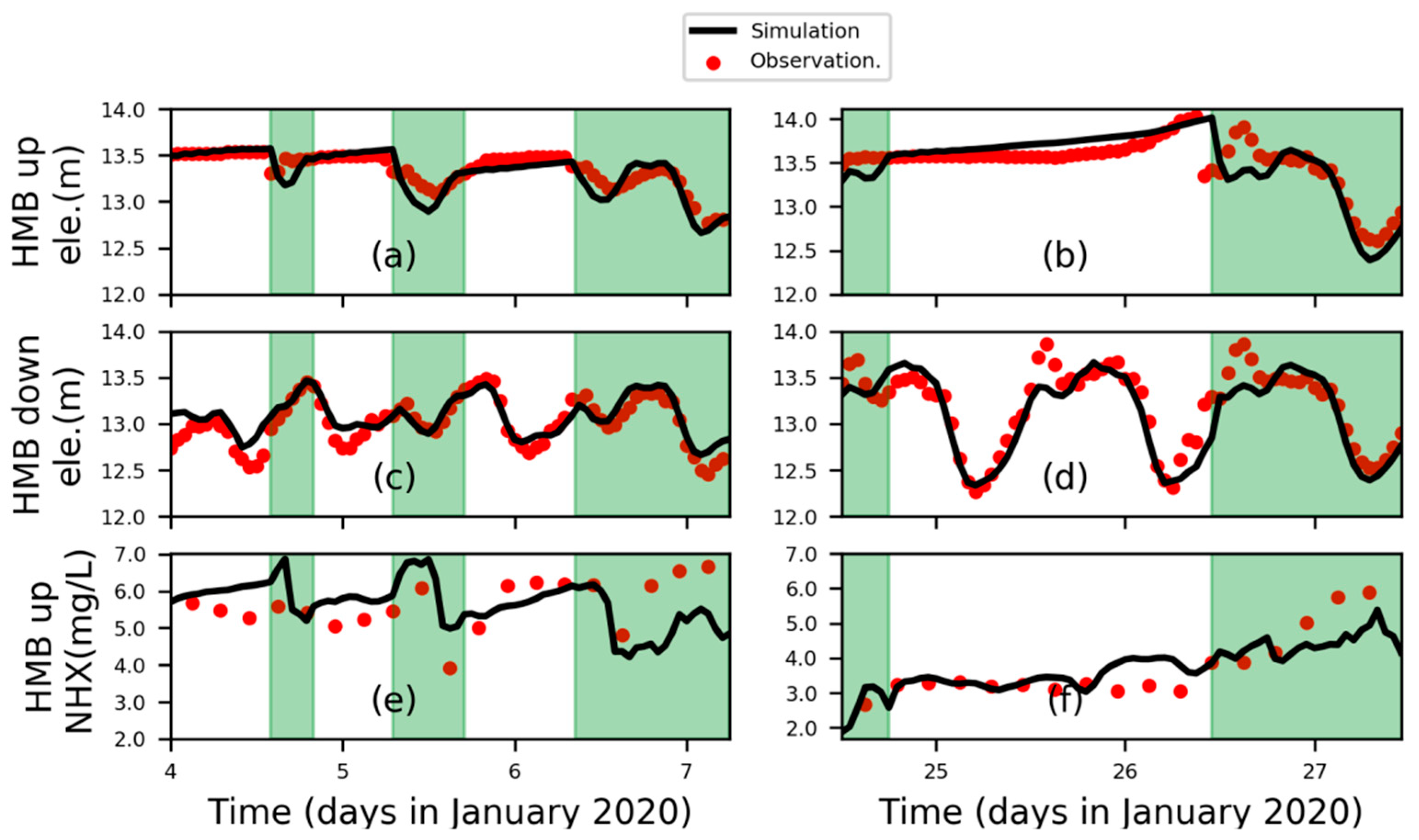
3.1. Validation
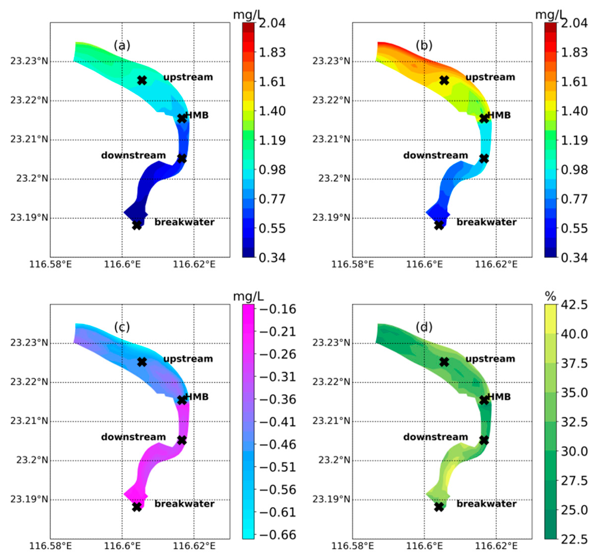
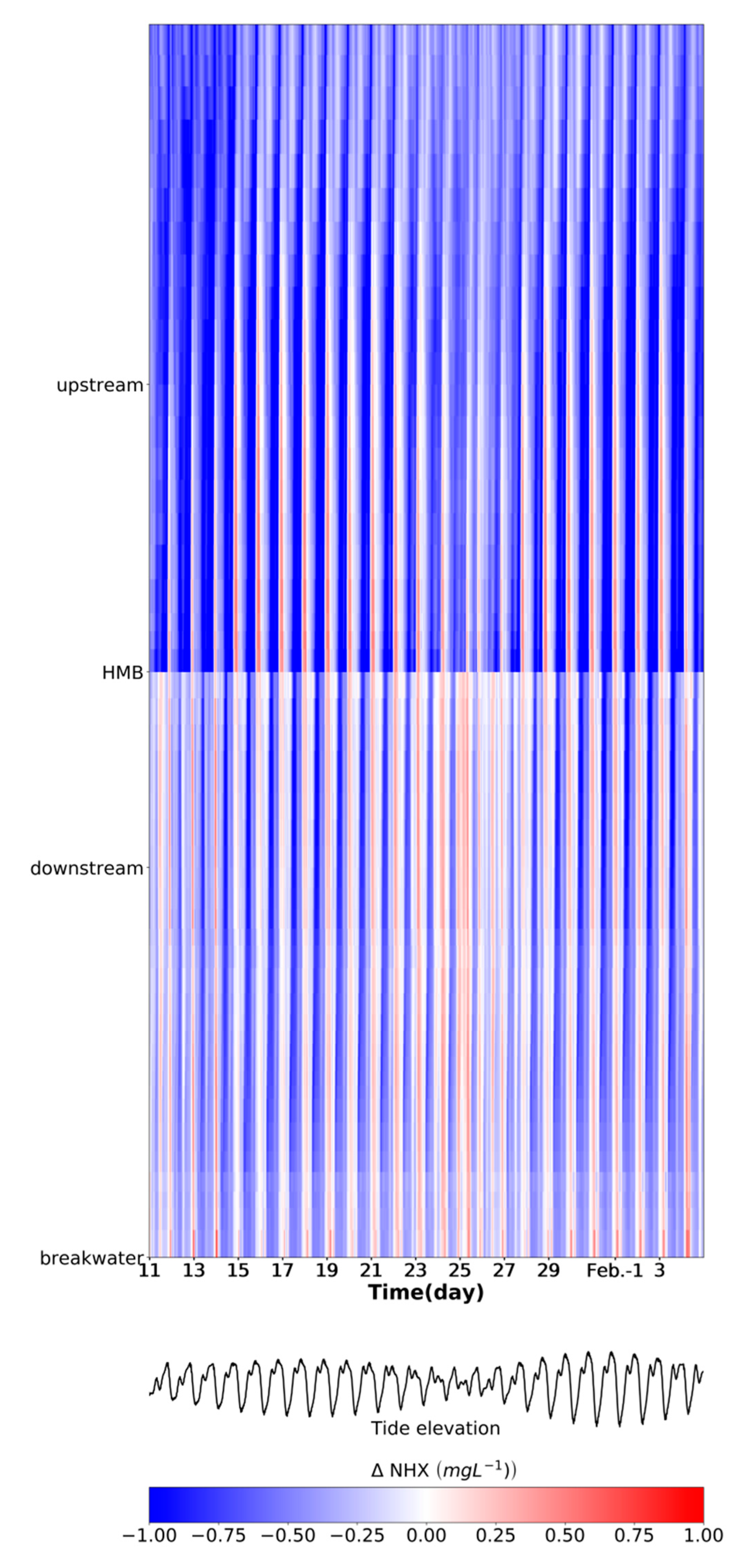
3.2. Variation of Ammonia Concentration
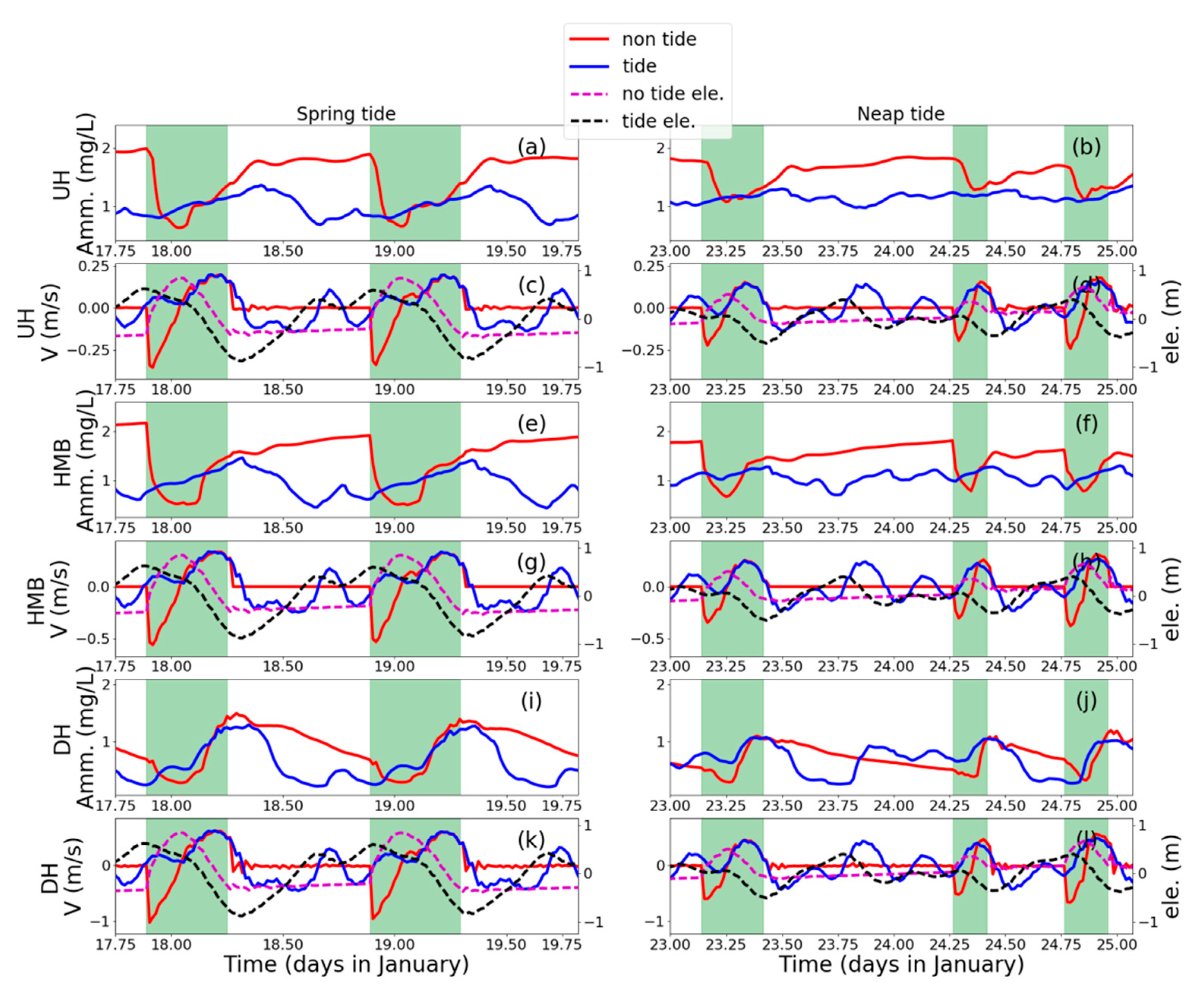
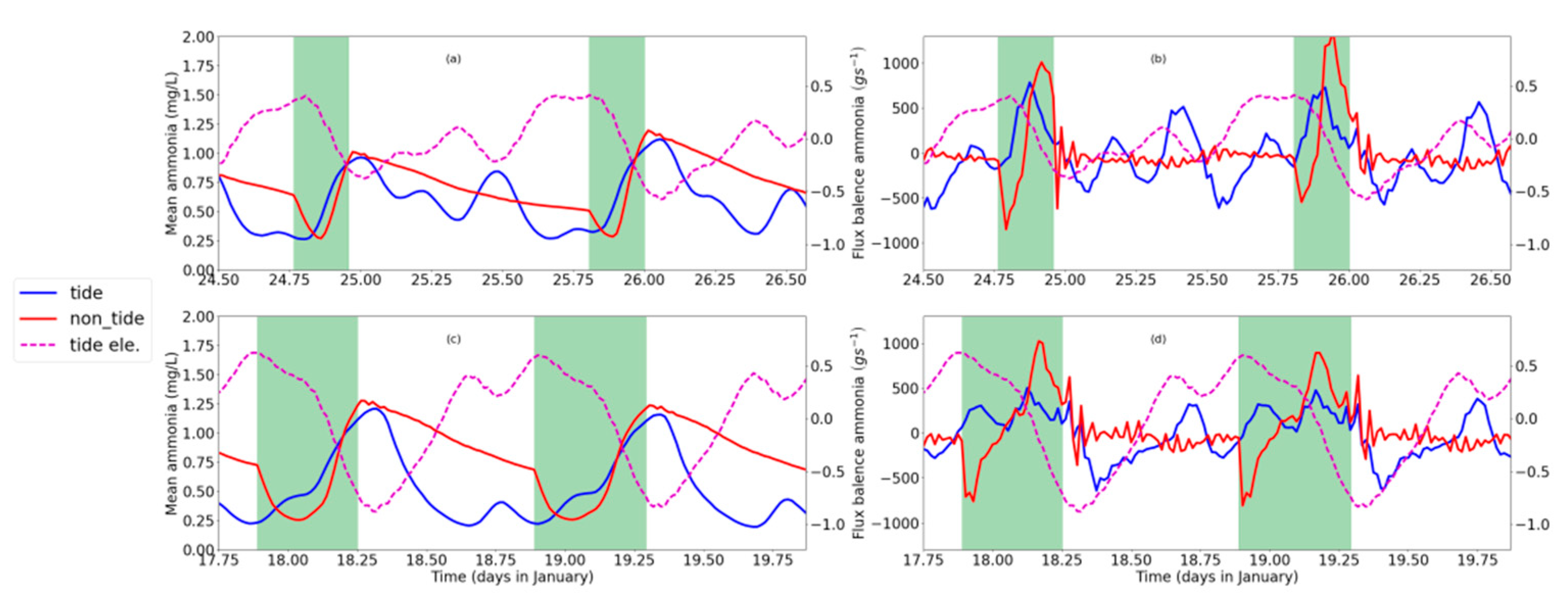
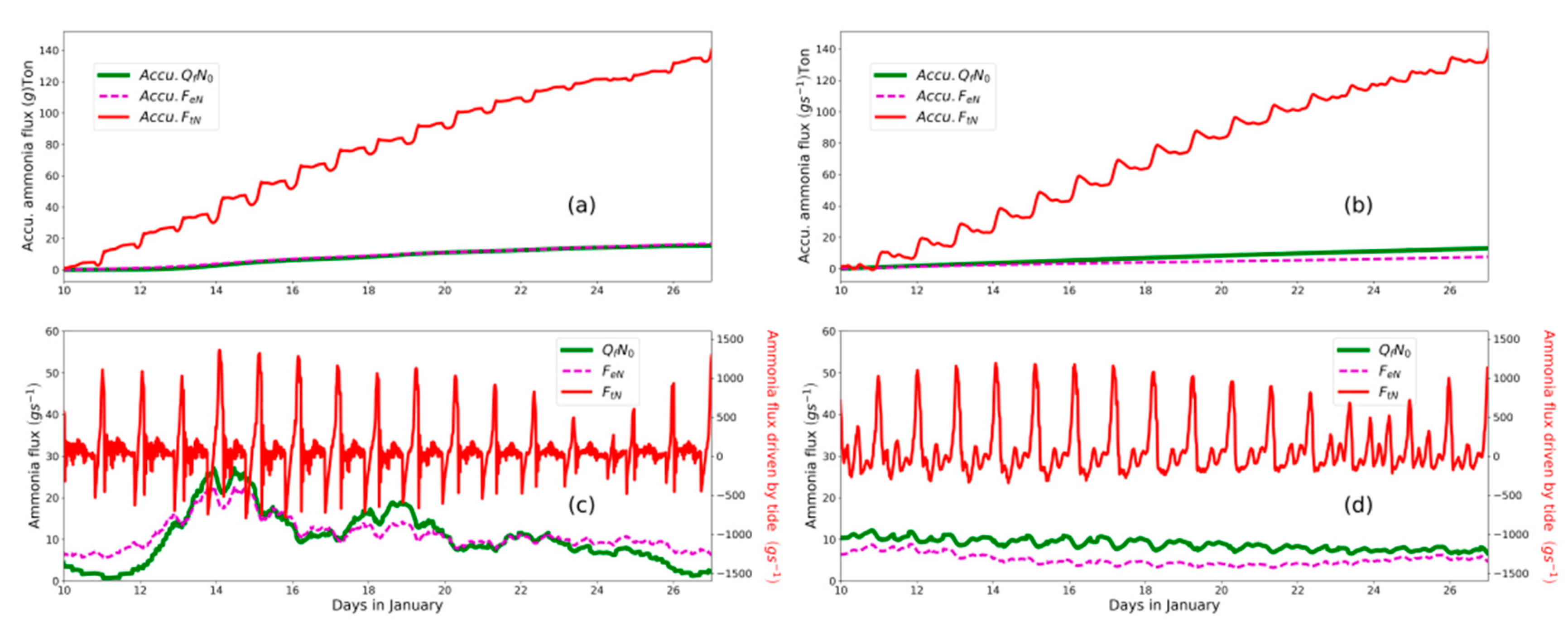
3.3. Variations in Time Series
4. Discussion
5. Conclusions
Author Contributions
Funding
Acknowledgments
Conflicts of Interest
References
- Elliott, M.; Whitfield, A.K. Challenging paradigms in estuarine ecology and management. Estuar. Coast. Shelf Sci. 2011, 94, 306–314. [Google Scholar] [CrossRef]
- Yanagi, T.; Ducrotoy, J.P. Toward coastal zone management that ensures coexistence between people and nature in the 21st century. Mar. Pollut. Bull. 2003, 47, 1–4. [Google Scholar] [CrossRef]
- Ysebaert, T.; van der Hoek, D.-J.; Wortelboer, R.; Wijsman, J.W.M.; Tangelder, M.; Nolte, A. Management options for restoring estuarine dynamics and implications for ecosystems: A quantitative approach for the Southwest Delta in the Netherlands. Ocean Coast. Manag. 2016, 121, 33–48. [Google Scholar] [CrossRef] [Green Version]
- Goodwin, C.R. Simulation of the Effects of Proposed Tide Gates on Circulation, Flushing, and Water Quality in Residential Canals, Cape Coral, Florida; US Geological Survey: Reston, VA, USA, 1991. [Google Scholar]
- Charland, J.W. Alternative tide gate designs for habitat enhancement and water quality improvement. In Proceedings of the Marine Environment Engineering Technology Symposium, Alexandria, VA, USA, 28–30 September 2001. [Google Scholar]
- Thomson, A.R. Study of Flood Proofing Barriers in Lower Mainland Fish Bearing Streams; Department of Fisheries and Oceans, Habitat and Enhancement Branch, Pacific Region: Vancouver, BC, Canada, 1999.
- Choudri, B.S.; Baawain, M.; Ahmed, M. Review of Water Quality and Pollution in the Coastal Areas of Oman. Pollut. Res. 2015, 34, 439–449. [Google Scholar]
- Paalvast, P.; van der Velde, G. Long term anthropogenic changes and ecosystem service consequences in the northern part of the complex Rhine-Meuse estuarine system. Ocean Coast. Manag. 2014, 92, 50–64. [Google Scholar] [CrossRef] [Green Version]
- Wright, G.V.; Wright, R.M.; Bendall, B.; Kemp, P.S. Impact of tide gates on the upstream movement of adult brown trout, Salmo trutta. Ecol. Eng. 2016. [Google Scholar] [CrossRef]
- Verdonschot, P.F.M.; Spears, B.M.; Feld, C.K.; Brucet, S.; Keizer-Vlek, H.; Borja, A.; Elliott, M.; Kernan, M.; Johnson, R.K. A comparative review of recovery processes in rivers, lakes, estuarine and coastal waters. Hydrobiologia 2013, 704, 453–474. [Google Scholar] [CrossRef]
- Choudhury, A.K.; Pal, R. Variations in seasonal phytoplankton assemblages as a response to environmental changes in the surface waters of a hypo saline coastal station along the Bhagirathi-Hooghly estuary. Environ. Monit. Assess. 2011, 179, 531–553. [Google Scholar] [CrossRef]
- Ducrotoy, J.P.; Elliott, M. Recent developments in estuarine ecology and management. Mar. Pollut. Bull. 2006, 53, 1. [Google Scholar] [CrossRef]
- Masselink, G.; Hanley, M.E.; Halwyn, A.C.; Blake, W.; Kingston, K.; Newton, T.; Williams, M. Evaluation of salt marsh restoration by means of self-regulating tidal gate – Avon estuary, South Devon, UK. Ecol. Eng. 2017, 106, 174–190. [Google Scholar] [CrossRef]
- Souder, J.A.; Tomaro, L.M.; Giannico, G.R.; Behan, J.R. Ecological Effects of Tide Gate Upgrade or Removal: A Literature Review and Knowledge Synthesis; Oregon State University: Corvallis, OR, USA, 2018. [Google Scholar]
- Li, S.; Zhang, Q. Risk assessment and seasonal variations of dissolved trace elements and heavy metals in the Upper Han River, China. J. Hazard. Mater. 2010, 181, 1051–1058. [Google Scholar] [CrossRef] [PubMed]
- Young, S.M.; Ishiga, H. Environmental change of the fluvial-estuary system in relation to Arase Dam removal of the Yatsushiro tidal flat, SW Kyushu, Japan. Environ. Earth Sci. 2014, 72, 2301–2314. [Google Scholar] [CrossRef]
- Chernetsky, A.S.; Schuttelaars, H.M.; Talke, S.A. The effect of tidal asymmetry and temporal settling lag on sediment trapping in tidal estuaries. Ocean Dyn. 2010, 60, 1219–1241. [Google Scholar] [CrossRef] [Green Version]
- Winterwerp, J.C. Fine sediment transport by tidal asymmetry in the high-concentrated Ems River: Indications for a regime shift in response to channel deepening. Ocean Dyn. 2011, 61, 203–215. [Google Scholar] [CrossRef] [Green Version]
- Ning, X.; Chai, F.; Xue, H.; Cai, Y.; Liu, C.; Shi, J. Physical-biological oceanographic coupling influencing phytoplankton and primary production in the South China Sea. J. Geophys. Res. C Ocean. 2004, 109. [Google Scholar] [CrossRef] [Green Version]
- Ou, S.; Zhang, H.; Wang, D.X.; He, J. Horizontal characteristics of buoyant plume off the Pearl River Estuary during summer. J. Coast. Res. 2007, SI50, 652–657. [Google Scholar]
- Yin, K.; Song, X.; Sun, J.; Wu, M.C.S. Potential P limitation leads to excess N in the pearl river estuarine coastal plume. Cont. Shelf Res. 2004, 24, 1895–1907. [Google Scholar] [CrossRef]
- Gan, J.; Li, L.; Wang, D.; Guo, X. Interaction of a river plume with coastal upwelling in the northeastern South China Sea. Cont. Shelf Res. 2009. [Google Scholar] [CrossRef]
- Jiang, C.; Cao, R.; Lao, Q.; Chen, F.; Zhang, S.; Bian, P. Typhoon Merbok induced upwelling impact on material transport in the coastal northern South China Sea. PLoS One 2020, 15, 1–15. [Google Scholar] [CrossRef]
- Jing, Z.Y.; Qi, Y.Q.; Hua, Z.L.; Zhang, H. Numerical study on the summer upwelling system in the northern continental shelf of the South China Sea. Cont. Shelf Res. 2009, 29, 467–478. [Google Scholar] [CrossRef] [Green Version]
- Li, W.; Lin, S.; Wang, W.; Huang, Z.; Zeng, H.; Chen, X.; Zeng, F.; Fan, Z. Assessment of nutrient and heavy metal contamination in surface sediments of the Xiashan stream, eastern Guangdong Province, China. Environ. Sci. Pollut. Res. 2019, 1–17. [Google Scholar] [CrossRef] [PubMed]
- Shen, J.; Lin, J. Modeling study of the influences of tide and stratification on age of water in the tidal James River. Estuar. Coast. Shelf Sci. 2006, 68, 101–112. [Google Scholar] [CrossRef]
- Arifin, R.R.; James, S.C.; de Alwis Pitts, D.A.; Hamlet, A.F.; Sharma, A.; Fernando, H.J.S. Simulating the thermal behavior in Lake Ontario using EFDC. J. Great Lakes Res. 2016, 42, 511–523. [Google Scholar] [CrossRef]
- Devkota, J.; Fang, X. Numerical simulation of flow dynamics in a tidal river under various upstream hydrologic conditions Numerical simulation of flow dynamics in a tidal river under various. Hydrol. Sci. J. 2015, 60, 1666–1689. [Google Scholar] [CrossRef]
- Zhu, L.; He, Q.; Shen, J.; Wang, Y. The influence of human activities on morphodynamics and alteration of sediment source and sink in the Changjiang Estuary. Geomorphology 2016, 273, 52–62. [Google Scholar] [CrossRef]
- Mellor, G.L.; Yamada, T. Development of a turbulence closure model for geophysical fluid problems. Rev. Geophys. 1982, 20, 851–875. [Google Scholar] [CrossRef] [Green Version]
- Hamrick, J.M. User’s Manual for the Environmental Fluid Dynamics Computer Work; Special Report in Applied Marine Science and Ocean Engineering No. 331; Virginia Institute of Marine Science/School of Marine Science, the College of William and Mary: Gloucester Point, VA, USA, 1996. [Google Scholar]
- Chapelle, A.; Lazure, P.; Ménesguen, A. Modelling eutrophication events in a coastal ecosystem. Sensitivity analysis. Estuar. Coast. Shelf Sci. 1994, 39, 529–548. [Google Scholar] [CrossRef]
- Guan, W.; Wong, L.-A.; Xu, D. Modelling nitrogen and phosphorus cycles and dissolved oxygen in the Zhujiang Estuary I. Model development. Acta Oceanol. Sin. 2001, 20, 493–504. [Google Scholar]
- Gharibi, H.; Mahvi, A.H.; Nabizadeh, R.; Arabalibeik, H.; Yunesian, M.; Sowlat, M.H. A novel approach in water quality assessment based on fuzzy logic. J. Environ. Manage. 2012, 112, 87–95. [Google Scholar] [CrossRef]
- Pawlowicz, R.; Beardsley, B.; Lentz, S. Classical tidal harmonic analysis including error estimates in MATLAB using TDE. Comput. Geosci. 2002, 28, 929–937. [Google Scholar] [CrossRef]
- Lerczak, J.A.; Geyer, W.R.; Chant, R.J. Mechanisms driving the time-dependent salt flux in a partially stratified estuary. J. Phys. Oceanogr. 2006, 36, 2296–2311. [Google Scholar] [CrossRef] [Green Version]
- Zhou, W.; Wang, D.; Luo, L. Investigation of saltwater intrusion and salinity stratification in winter of 2007/2008 in the Zhujiang River Estuary in China. Acta Oceanol. Sin. 2012, 31, 31–46. [Google Scholar] [CrossRef]
- Kärnä, T.; Baptista, A.M. Water age in the Columbia River estuary. Estuar. Coast. Shelf Sci. 2016, 183, 249–259. [Google Scholar] [CrossRef] [Green Version]
- Warner, J.C.; Geyer, W.R.; Lerczak, J.A. Numerical modeling of an estuary: A comprehensive skill assessment. J. Geophys. Res. C Ocean. 2005, 110, 1–13. [Google Scholar] [CrossRef]
- Bowen, M.M.; Geyer, W.R. Salt Transport and the Time-dependent Salt Balance of a Partially Stratified Estuary. J. Geophys. Res.Oceans 2003. [Google Scholar] [CrossRef]
- Lerczak, J.A.; Geyer, W.R.; Ralston, D.K. The temporal response of the length of a partially stratified estuary to changes in river flow and tidal amplitude. J. Phys. Oceanogr. 2009, 39, 915–933. [Google Scholar] [CrossRef] [Green Version]
- Romero, E.; Garnier, J.; Billen, G.; Ramarson, A.; Riou, P.; Le Gendre, R. Modeling the biogeochemical functioning of the Seine estuary and its coastal zone: Export, retention, and transformations. Limnol. Oceanogr. 2019, 64, 895–912. [Google Scholar] [CrossRef]
- Peierls, B.L.; Hall, N.S.; Paerl, H.W. Non-monotonic responses of phytoplankton biomass accumulation to hydrologic variability: A comparison of two coastal plain north carolina estuaries. Estuaries Coasts 2012, 35, 1376–1392. [Google Scholar] [CrossRef]
- Cloern, J.E.; Foster, S.Q.; Kleckner, A.E. Phytoplankton primary production in the world’s estuarine-coastal ecosystems. Biogeosciences 2014, 11, 2477. [Google Scholar] [CrossRef] [Green Version]


| Variable | Station | Time | |||
|---|---|---|---|---|---|
| 2020.1.4–1.7 | 2020.1.24–1.27 | ||||
| r | SS | r | SS | ||
| Elevation | HMB up | 0.87 | 0.96 | 0.89 | 0.95 |
| Elevation | HMB down | 0.85 | 0.93 | 0.90 | 0.95 |
| Ammonia | HMB up | 0.20 | 0.38 | 0.41 | 0.15 |
| Sections | Variable | Concerned Time Period | Neap Tide | Non-Tide | Spring–Neap Cycle | ||
|---|---|---|---|---|---|---|---|
| Spring Tide | Non-Tide | Tide | Non-Tide | ||||
| HMB | Ammonia Flux Seaward | (Ton/Lunar Cycle) | (Ton/Spring–Neap Cycle) | ||||
| 10.52 | 13.15 | 4.52 | 8.56 | 126.23 | 165.65 | ||
| Breakwater | 10.85 | 10.45 | 6.74 | 7.93 | 135.52 | 144.46 | |
| HMB | Flux Seaward | (104 m3/Lunar Cycle) | (104 m3/spring–neap cycle) | ||||
| 196.77 | 379.86 | −40.08 | 361.46 | 12,623.16 | 16,565.13 | ||
| Breakwater | 219.34 | 146.91 | −66.88 | 200.89 | 13,551.69 | 14,446.32 | |
© 2020 by the authors. Licensee MDPI, Basel, Switzerland. This article is an open access article distributed under the terms and conditions of the Creative Commons Attribution (CC BY) license (http://creativecommons.org/licenses/by/4.0/).
Share and Cite
Zhao, C.; Yang, H.; Fan, Z.; Zhu, L.; Wang, W.; Zeng, F. Impacts of Tide Gate Modulation on Ammonia Transport in a Semi-closed Estuary during the Dry Season—A Case Study at the Lianjiang River in South China. Water 2020, 12, 1945. https://doi.org/10.3390/w12071945
Zhao C, Yang H, Fan Z, Zhu L, Wang W, Zeng F. Impacts of Tide Gate Modulation on Ammonia Transport in a Semi-closed Estuary during the Dry Season—A Case Study at the Lianjiang River in South China. Water. 2020; 12(7):1945. https://doi.org/10.3390/w12071945
Chicago/Turabian StyleZhao, Changjin, Hanjie Yang, Zhongya Fan, Lei Zhu, Wencai Wang, and Fantang Zeng. 2020. "Impacts of Tide Gate Modulation on Ammonia Transport in a Semi-closed Estuary during the Dry Season—A Case Study at the Lianjiang River in South China" Water 12, no. 7: 1945. https://doi.org/10.3390/w12071945