Measurement of Total Nitrogen Concentration in Surface Water Using Hyperspectral Band Observation Method
by
 ,
,
Changjiang Liu
1,2, 
Fei Zhang
1,2,3,4,*,
Xiangyu Ge
1,2 ,
,
Xianlong Zhang
1,2,
Ngai weng Chan
5 and 
Yaxiao Qi
1,2 1
Key Laboratory of Wisdom City and Environment Modeling of Resources and Environmental Science College, Urumqi 830046, China
2
Key Laboratory of Oasis Ecology, Xinjiang University, Urumqi 830046, China
3
Engineering Research Center of Central Asia Geoinformation Development and Utilization, National Administration of Surveying, Mapping and Geoinformation, Urumqi 830002, China
4
Commonwealth Scientific and Industrial Research Organization Land and Water, Canberra ACT 2601, Australia
5
School of Humanities, Universiti Sains Malaysia, George Town, Penang 11800, Malaysia
*
Author to whom correspondence should be addressed.
Water 2020, 12(7), 1842; https://doi.org/10.3390/w12071842
Submission received: 23 April 2020
/
Revised: 11 June 2020
/
Accepted: 18 June 2020
/
Published: 27 June 2020
Abstract
:Nitrogen overload is one of the main reasons for the deterioration of surface water quality. Hence, monitoring nitrogen loadings is vital in maintaining good surface water quality. Increasingly, the use of spectral reflectance to monitor nitrogen concentration in water has shown potentials, but it poses some problems. Therefore, it is necessary to explore new methods of quantitative monitoring of nitrogen concentration in surface water. In this paper, hyperspectral data from surface water in the Ebinur Lake watershed are used to select sensitive bands using spectral transformation, the spectral index, and a coupling of these two methods. The particle swarm optimization support vector machine (PSO-SVM) model, constructed on the basis of sensitive bands, is used quantitatively to estimate the total nitrogen concentration in surface water and subsequently to verify its accuracy. The results show that the bands near 680, 850, and 940 nm can be used as sensitive bands for estimation of the total nitrogen concentration of surface water in arid regions. Compared with the best estimation models constructed by sensitive bands selected using the spectral transformation or the spectral index alone, the best model based on the coupling of these two measures is more accurate (R2 = 0.604, Root Mean Square Error (RMSE) = 1.61 mg/L, Residual Prediction Deviation (RPD) = 2.002). This coupling method leads to a robust, accurate, and strong predictability model, and can contribute to improved quantitative estimation of water quality indexes of rivers in arid regions.
1. Introduction
Excessive nitrogen concentration is one of the main water pollution problems in Chinese rivers as well as rivers worldwide [1,2,3]. Excessive nitrogen in rivers feed algae causing it to grow faster than what most river ecosystems can handle. The result is the occurrence of eutrophication caused by large algal blooms which can consume almost all the oxygen in a river, producing so-called “dead zones” [4]. Rivers devoid of oxygen leads to hypoxia which kills virtually all aquatic organisms in the river, rendering the river to be declared as a “dead river”. The main reason for the increase of the nitrogen concentration in inland waters is the intensification of industrial and agricultural activities, with their resulting effluents and pollutants discharging into waterways leading to severe ecological and environmental problems [5]. In China, it was reported that the Yangtze and Pearl river estuaries have been turned into dead zones, mostly due to nitrogen pollution of the waterways [6]. Most alarmingly, dangerous toxins are produced by harmful algal blooms (HABs) and these directly threaten human health [7]. Hence, it is of paramount importance that nitrogen pollution of surface waters be controlled to minimize all these problems.
Although satellite remote sensing can support extensive spatial and temporal monitoring, it has obvious disadvantages such as serious information redundancy, low spatial–temporal resolution and difficulty in quantitative inversion of water quality indexes in small rivers. Surface hyperspectral remote sensing technology can not only distinguish various spectral of water bodies to extract rich information but also have a controllable time resolution and high mobility, which can result in high-precision quantitative inversion of water quality indicators in small rivers [8]. However, the quantitative study of water quality indexes mainly focuses on the estimation of light sensitive variables, such as total suspended solids, chlorophyll-a and turbidity, while use of hyperspectral data to study other water quality indexes that are insensitive to light, such as total nitrogen, pH, and dissolved phosphorus, is rarely implemented [9]. Quantitative estimation methods for the total nitrogen concentration in surface water by hyperspectral data mainly include direct methods [10,11,12], indirect methods [13,14,15], and physicochemical methods [16,17,18].
To date, quantitative estimation of the total nitrogen concentration in surface water directly using hyperspectral data is still rare [19], especially in arid regions. Due to geographical factors, the water quality indices of surface water are often quite variable. Although various analysis and modelling methods are used in water quality index inversion and have achieved good results, they inevitably result in new errors when applied to new regions. In the arid regions, the applicability of the quantitative estimation model of total nitrogen concentration in surface water has yet to be verified due to the influence of special environmental conditions. However, the total nitrogen concentration of water is one of the most important water quality indicators. It has a profound impact on the water quality in arid regions, and it is also a challenging field for its high-precision estimation [20,21]. Therefore, it is necessary to develop a quantitative monitoring method suitable for arid regions, which is of practical significance for solving the ecological and environmental problems caused by nitrogen pollution.
The measured hyperspectral data can be used to estimate the total nitrogen concentration in water, but the hyperspectral data’s information is always huge. If the original data is directly used in the calculation, it will cause the serious Hughes phenomenon [22]. Hence, the application of hyperspectral data is limited. Sensitive band selection is a common method to effectively reduce the dimension of hyperspectral data, which can significantly reduce the Hughes phenomenon. We summarize the most advanced band selection methods, which can be divided into six categories, i.e., searching based, clustering based, deep-learning-based, ranking based, sparsity based, and hybrid-scheme based methods [23,24]. These methods have many advantages, but there are also some defects. For example, although the first three methods are suitable for small samples, they usually have higher computational costs. The ranking based method is only suitable for large data sets, and the sparsity based method requires the imposing of sparse constraints. However, spectral transformation and spectral index can effectively enhance spectral information, which can be used in the selection of sensitive bands. In view of this, this paper attempts to couple spectral transformation and spectral index to achieve the purpose of optimizing sensitive bands on the basis of screening sensitive bands by spectral transformation and spectral index respectively.
In this study, the main three rivers in the Ebinur Lake watershed, located in XinJiang, China, were selected (Figure 1), because they are under the influence of large-scale agricultural and relatively concentrated industrial activities. The aims of this paper are to: (1) collect data on the hyperspectral reflectance of surface water and select sensitive bands based on spectral transformation and the spectral index, (2) attempt to couple spectral transformation and the spectral index to optimize the sensitive bands, (3) establish a PSO-SVM model based on the sensitive bands to quantitatively estimate the total nitrogen concentration of surface water, and (4) compare the inversion accuracy of the PSO-SVM model based on three methods for selecting sensitive bands.
2. Materials and Methods
2.1. Study Area
The Ebinur Lake watershed (43°38′–45°52′ N and 79°53′–85°02′ E) is located in northwest Xinjiang, China (Figure 1). The study area is about 50,621 km2, comprising Bortala River Valley, Jinghe oasis, Wusu Oasis, Dandagai desert, and Mutetaer desert zone of the lower reaches of the Akeqisu–Kuitun River. The Ebinur Lake is located in the lowest elevation of the watershed and is the largest saltwater lake in Xinjiang. It has the characteristics of a typical lake in the arid region of Central Asia. The area experiences a typical arid continental climate in the middle temperate zone and is characterized by drought, low rainfall, drastic temperature variations, and severe soil salinization [25].
Three rivers, the Bortala, Jinghe, and Kuitun Rivers, flow into Ebinur Lake from the south, and west and east, respectively, and constitute the main water sources of the watershed. There are a lot of farmlands in the Bortala River, Jinghe River, and Kuitun River Sub watersheds, and some artificial reservoirs are constructed in the southwest of the Ebinur Lake. Over the past 40 years, due to the impact of human irrigation activities, the water inflow into the lake from these three rivers has decreased significantly. This has consequently lowered the water level of the lake, dropping it by 2–3 m, resulting in the reduction of the lake surface to less than 500 km2, and deterioration of the water environment of the watershed [26].
2.2. Measured Spectral Data and Preprocessing
Surface water hyperspectral data from the Bortala, Jinghe, and Kuitun Rivers were collected between October 12 and October 20, 2017. Based on the measured spectral curves, 3 groups of abnormal curves were eliminated, and 32 groups of hyperspectral curves were retained.
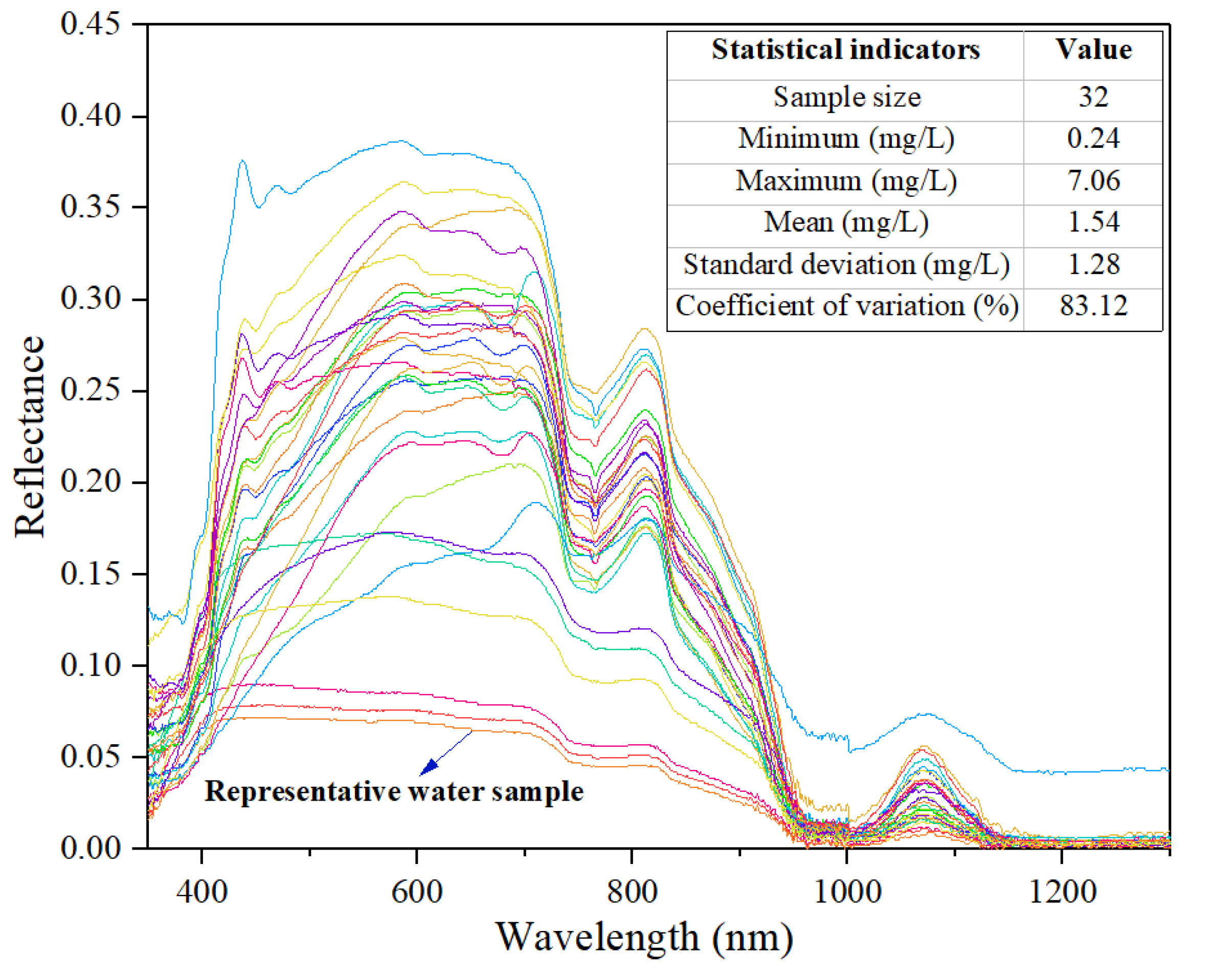
A UV-VIS Spectro Photometer (UV-6100, mapada, Shanghai, China) was used to measure the total nitrogen concentration [27]. Before the test, instrument self-inspection and calibration were performed. During the test, the solution in the cuvette was 2/3–4/5 higher than the cuvette and kept clean. Three parallel water samples were collected from each sampling point to measure the total nitrogen concentration, and the mean value of the total nitrogen concentration of the three samples was taken as the measured value. The basic statistics of the test results are shown in the table in the upper right corner of Figure 2. In order to further describe the total nitrogen concentration of surface water in Ebinur Lake watershed, referring to the standard values of the Ⅲ and Ⅴ categories of water in the environmental quality standard for surface water (GB3838-2002), we divided the measured data into three levels: low nitrogen concentration (0–1 mg/L), medium nitrogen concentration (1–2 mg/L), and high nitrogen concentration (2–7.06 mg/L). Based on the measured results, there are 14 samples with low nitrogen concentration, 8 samples with medium nitrogen concentration, and 10 samples with high nitrogen concentration in the total 32 water samples. To ensure representative training and verification sets, 4 samples of low concentration, 2 samples of medium concentration, and 2 samples of high concentration were randomly selected from three concentration levels as verification set, and the rest were used as training set.
An ASD fieldspec3 ground object spectrometer (Analytical Spectral Devices, Boulder, CO, USA) with a spectral range of 350–2500 nm was used to measure spectra [28]. Clear and windless weather was selected for field measurements, and the time of measurement time was 12:00–16:00 in the eastern six areas, facing the sun, to ensure that the sensor probe was vertical to the water surface. Before the test, white board correction was performed, and the mean value of 10 spectral curves collected from each water sample point was taken as the actual measured spectral curve for each point. To eliminate the influence of noise on the spectral data, the mean filtering method was used to uniformly denoise and smoothen the spectral curve [29]. The processed curves were taken as the characteristic spectral curves for each test water sample.
Nitrogen concentration is the main cause of eutrophication, and the degree of eutrophication is positively correlated with spectral reflectance [30,31], which is also substantiated by our measurement (Figure 2). Therefore, the water sample with lowest reflectance was selected to search for the sensitive band, which ensures the universality of the search method for the sensitive band to other water samples.
2.3. Spectral Transformation
Spectral transformation is an important means of spectral sensitive band analysis. Appropriate spectral transformation can effectively enhance the prediction accuracy and robustness of the model. In this paper, 14 spectral transformations are used to search for sensitive bands related to total nitrogen concentration in surface water. (Table 1).
2.4. Spectral Index Construction
The spectral index or improved spectral index are a common method for selecting a sensitive band for measuring a water quality index. Difference index (DI), ratio index (RI), and normalized difference index (NDI) are three kinds of remote sensing earth observation indices that are widely used and have high accuracy [32]. Based on these three index calculation formulas, the spectral difference index (SDI), spectral ratio index (SRI), and spectral normalized difference index (SNDI) were constructed to select sensitive bands from hyperspectral data (Table 2). By analysing the quantitative relationship between the sensitive bands and the measured values for the water nitrogen concentration, the optimal spectral index was selected to screen the sensitive bands, establishing an inversion model to improve the estimation efficiency and accuracy of the total nitrogen concentration.
2.5. PSO-SVM Model
The particle swarm optimization (PSO) algorithm is a kind of grouping based on optimization technology. This algorithm has received wide attention by the academic community because of its easy implementation, fast convergence, high accuracy, and applicability to small samples. In this study, the number of samples is small (32), which is the main reason for choosing this algorithm. The PSO algorithm regards every object to be optimized as a particle with an initial velocity and finds an optimal solution through iteration. After the PSO algorithm is initialized to a group of random particles, the corresponding random solution will be obtained, and then the optimal solution will be found through iteration. In each iteration, particles update themselves by tracking two extremum: the first is the optimal solution found by the particles themselves, which is called individual extremum; the other is the optimal solution found by the whole population present, which is the global extremum. In each iteration, particles update their speed and position through individual and group extremum, that is:
where w is the inertia weight, d is the space dimension, and i = 1,2...n, k is the current iteration number; xid, vid is the particle position and speed; pid is the particle individual optimal position, pgd is the global optimal solution; c1 and c2 are acceleration factors; and r1 and r2 are random numbers distributed in [0,1] interval. In the specific operation process, we set n = 32, c1 = 2, c2 = 2, w = 0.6, the maximum number of cycles as 500, and other super parameters as default value.
Therefore, the PSO algorithm can be applied to the optimization of a support vector machine (SVM). That is, the PSO algorithm can be used to find the optimal parameters of a SVM—the penalty coefficient C and kernel function parameter g, and construct a PSO-SVM [35] estimation model.
2.6. Evaluation Indices
To quantify the performance of the model, the decision coefficient (R2), mean square error (RMSE), and residual prediction deviation (RPD) were used to evaluate the inversion results. Similar studies have shown that this process is reliable [36,37]. The formulas are as follows:
where yi is the measured value, Yi is the predicted value, Ti is the average of the measured values of all samples, n is the number of soil samples, and SD is the standard deviation of the samples. R2 reflects the robustness of the model establishment and prediction. The larger the value of R2, the more robust the model and the higher the fitting degree of the estimation model. The RMSE is used to evaluate the inversion ability of the model. The smaller the value of the RMSE, the stronger the inversion ability of the model. RPD is used to evaluate the prediction ability of the model. When RPD is less than 1.4 mg/L, the model is not predictive. When RPD is between 1.4 mg/L and 2 mg/L, the model can make approximate quantitative predictions. When RPD exceed 2.0 mg/L, the model can perfectly complete a quantitative prediction.
3. Results and Analysis
3.1. Selection of Sensitive Bands Based on Spectral Transformation
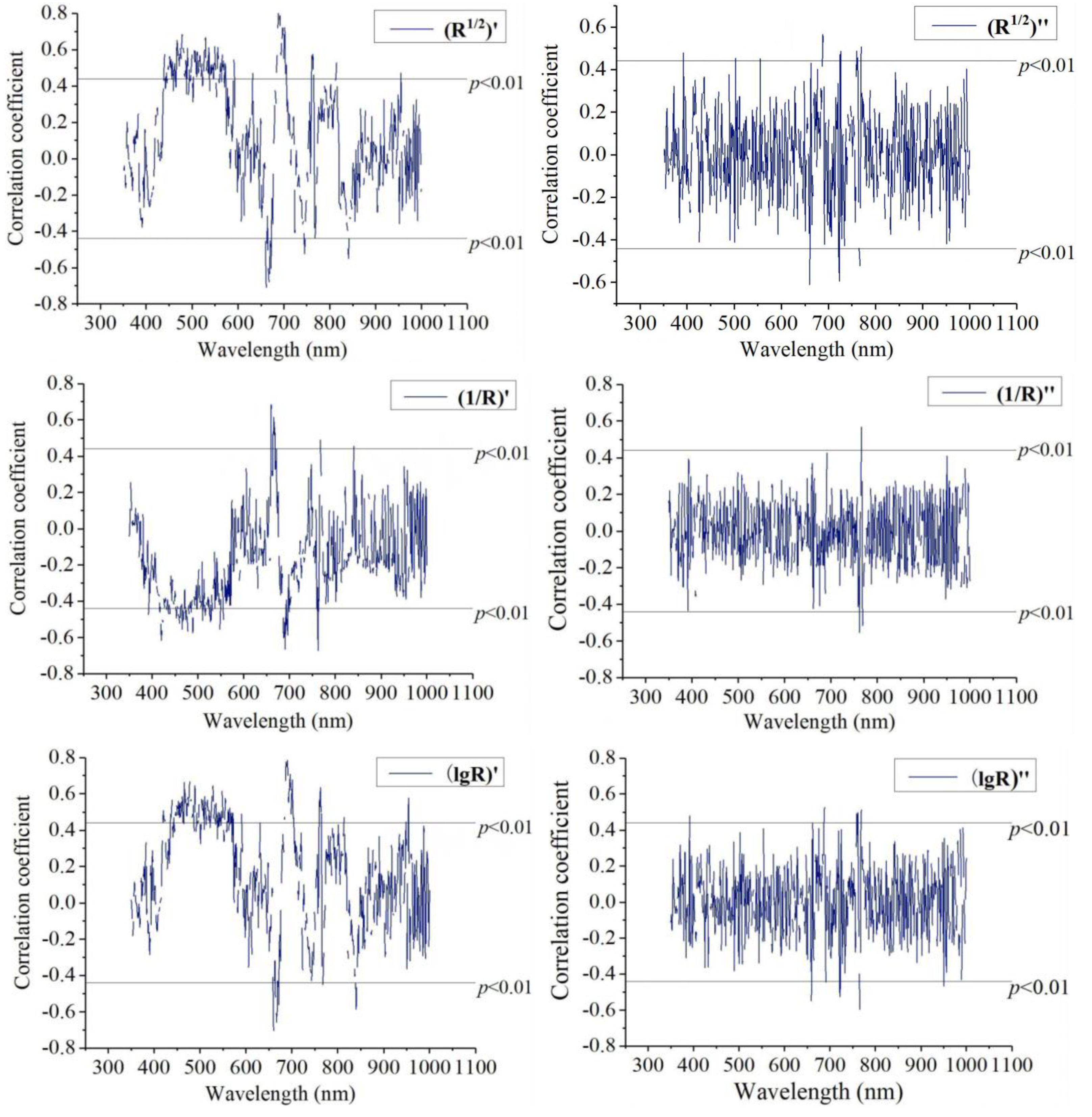
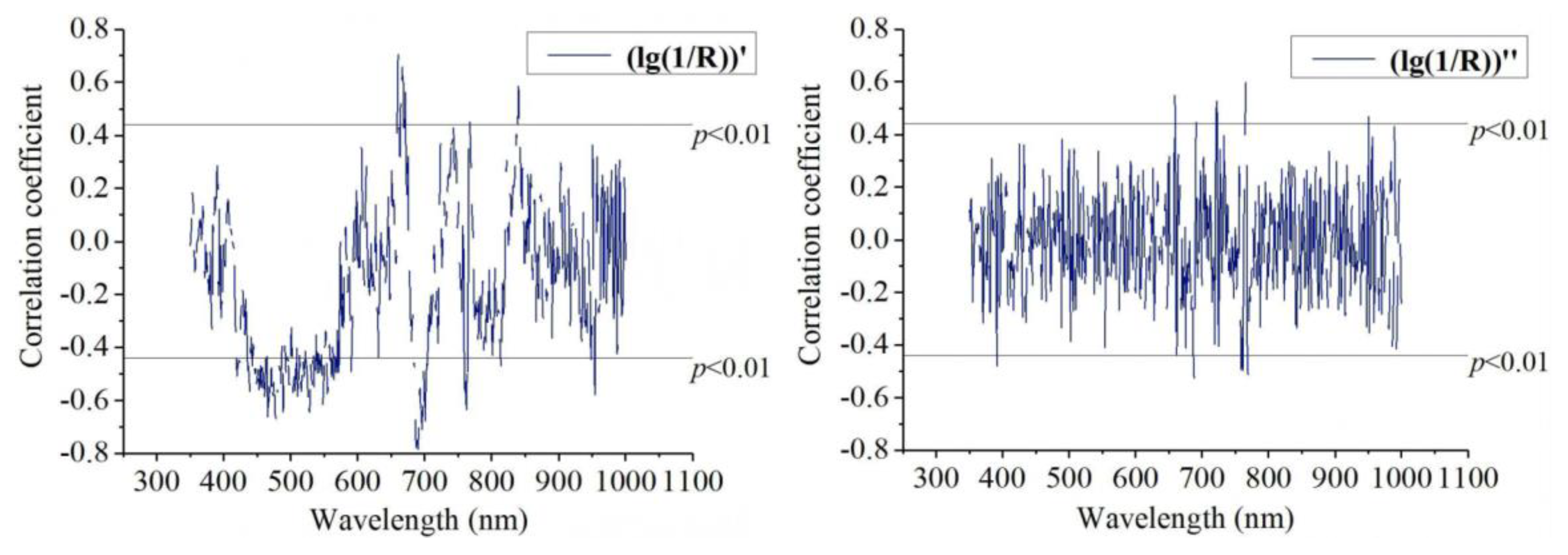
To improve the spectral sensitivity and highlight the mixed characteristic information of the spectral curve, 14 spectral transformations (Table 1) were carried out on the basis of the original spectral curve R, after denoising and smoothing. The partial correlation between the reflectance and the total nitrogen concentration was analysed to find the sensitive band. After screening, it was found that the first and second order differential forms of R1/2, 1/R, lgR, and lg(1/R) were significantly correlated with the measured total nitrogen concentration of surface water (Figure 3).
The black line in the figure indicates the critical value of the significance of correlation coefficient when the significance level is p = 0.01. The point above the critical value indicates that the band reflectance had a significant positive correlation with the total nitrogen concentration of water body, and the point below the critical value indicates a significant negative correlation. Here, we retain two bands corresponding to the correlation coefficient with larger absolute value as the combination of sensitive bands. Thus, the sensitive band for estimating the total nitrogen concentration of surface water was selected, as shown in Table 3. It can be seen that the absolute value of correlation coefficient varied from 0.54 to 0.8, and the spectral transformation form with better correlation was (R1/2)′ and (lg(1/R))′.
3.2. Selection of the Sensitive Band Based on the Spectral Index
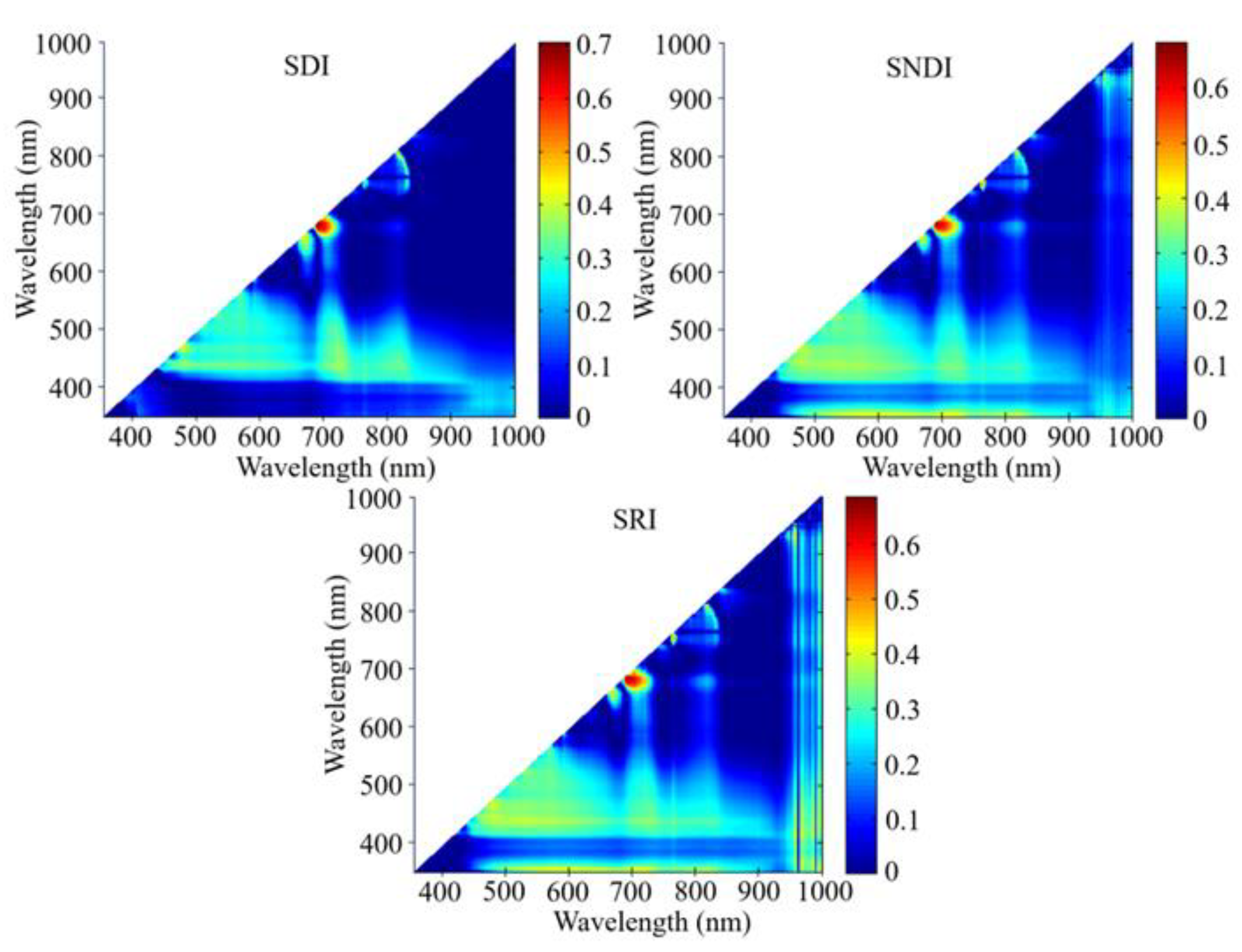
The spectral reflectance of water samples was arranged in a two-dimensional matrix sequence. The abscissa and ordinate axes were set as the spectral reflectance Ri and Rj, respectively, and the total nitrogen concentration in water samples was recorded as N. Matlab-R2012a software was used to construct a hyperspectral matrix coefficient map of the spectral reflectance and total nitrogen concentration in water (Figure 4) to evaluate the correlation between SDI, SRI, SNDI, and the total nitrogen concentration and to optimize the combination of sensitive bands significantly related to the total nitrogen concentration [38]. Different colours in the figures show the degree of correlation between the measured values of the total nitrogen concentration and the spectral index, the redder the color, the stronger the correlation. This kind of two-dimensional matrix map can accurately extract the effective peak wavelength with high correlation.
It can be seen from the hyperspectral matrix coefficient diagram that the three hyperspectral matrix coefficient diagrams (SDI, SRI, and SNDI) have similar distribution characteristics and are significantly related to the total nitrogen concentration of the water bodies under study. The sensitive bands and correlation coefficients related to the total nitrogen concentration of water bodies in different spectral indexes are shown in Table 4. We can see that the correlation coefficient based on the three spectral indices is relatively close, but the correlation coefficient based on SDI is the largest, with a value of 0.71.
3.3. Estimation of the Total Nitrogen Concentration in Surface Water
3.3.1. Estimation of the Total Nitrogen Concentration in Surface Water Based on Spectral Transformation and the Spectral Index
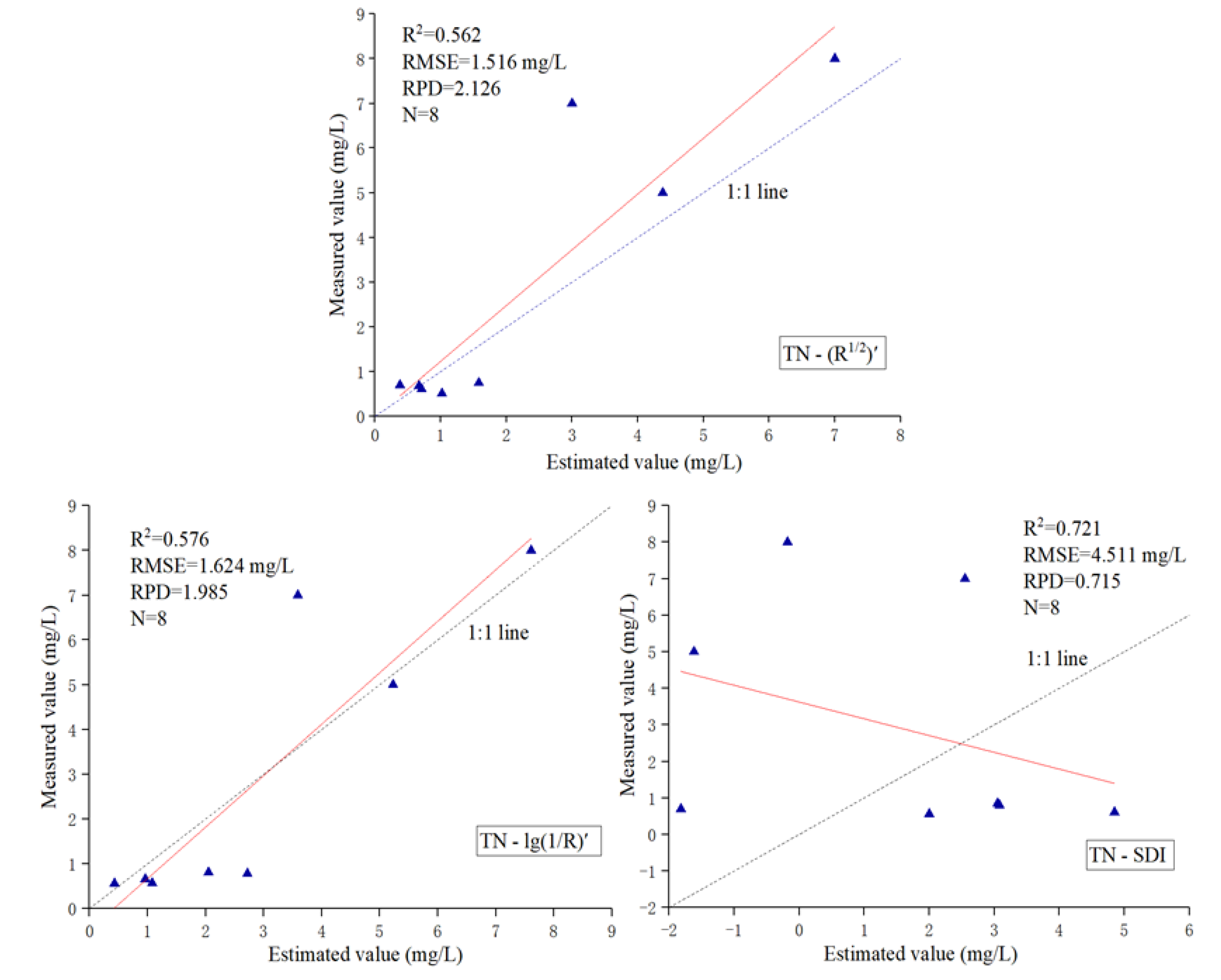
After the parameters C and g of the SVM were obtained by PSO, the spectral reflectance values of the sensitive bands of training and validation sets were taken as input variables and the measured total nitrogen concentration values of corresponding samples were taken as output variables. The total nitrogen concentration of each sample was obtained through an SVM machine learning algorithm and then its estimation accuracy was evaluated. According to Section 2.6, the larger of R2, RPD, and the smaller of RMSE, the higher of the model accuracy. From the results of the training set, the accuracy index of the model was persuasive, with R2, RMSE, and RPD values of 0.68–0.82, 0.62–0.93 mg/L, and 3.15–4.71, respectively. From the results of the validation set, the models based on (R1/2)′ and (lg(1/R))’ spectral transformations had approximately equal accuracies for estimating the total nitrogen concentration, but as can be seen in Figure 5, the model estimation accuracy under the (lg(1/R))′ spectral transformation was more reasonable, with R2, RMSE, and RPD values of 0.576, 1.624 mg/L, and 1.985, respectively. This finding provides an available model for the estimation of total nitrogen concentration in surface water, but its robustness and predictability are not ideal. In the estimation model based on the spectral index, the model constructed by the sensitive band selected using the SDI spectral index had the highest accuracy, with R2 of 0.721, RMSE value of 4.511 mg/L, and RPD of 0.715, but the R2 of the other two spectral indexes was lower than that of the spectral transformation. Therefore, it is not an ideal model for quantitative estimation of nitrogen concentration in surface water either. The accuracy of PSO-SVM estimation model based on the optimized spectral transformation and spectral index is shown in Figure 5 and Table 5.
3.3.2. Estimation of the Total Nitrogen Concentration in Surface Water Based on Spectral Transformation and Spectral Index Coupling
Based on the first-order and second-order differential transformations of lgR, 1/R, lg1/R, and R1/2, a number of sensitive bands that were significantly related to the total nitrogen concentration were selected. Subsequently, the PSO-SVM model was used to estimate the total nitrogen concentration. It was found that the estimation model using (R1/2)′ and (lg(1/R))′ spectral transformations estimated the total nitrogen concentration well, but the accuracy indexes R2 of these models only ranged between 0.5 and 0.6, suggesting that their estimation accuracy was limited. The estimation models built using the three spectral indexes SDI, SRI, and SNDI were also weak, with the maximum value of the determination coefficient R2 of 0.721, the RMSE was as high as 4.511 mg/L, and RPD was only 0.715.
Here, it can clearly be seen that the estimation model under (R1/2)′ and (lg(1/R))′ spectral transformation had smaller R2, but better RMSE and RPD; in contrast, the model under SNDI spectral index had larger R2, but worse RMSE and RPD (Table 5). In order to find a way to inherit the advantages of the above two methods, the next step was to develop a more effective method to improve the accuracy of total nitrogen concentration estimation.
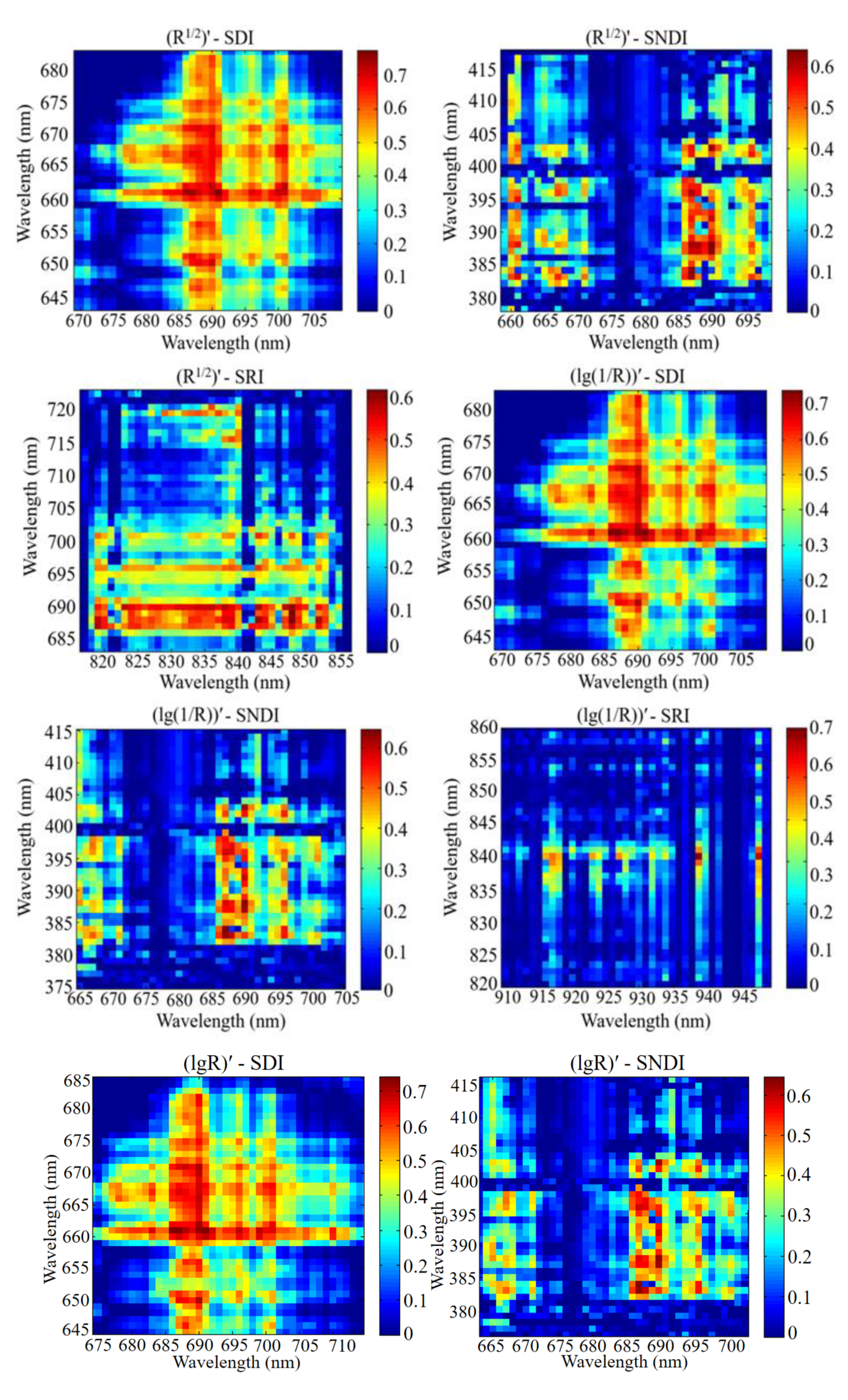
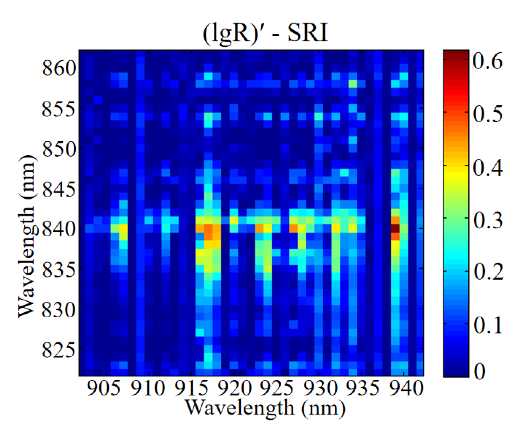
In view of this, an attempt was made to turn the spectral reflectance of (R1/2)′, (lg(1/R))′, and lg(R)′ into a two-dimensional matrix sequence and then nested them in three spectral index modules, SDI, SRI, and SNDI, using Matlab-R2012a software to build the hyperspectral matrix coefficient map of the spectral transformation and spectral index coupling (Figure 6). The hyperspectral sensitive band combination with a high autocorrelation to the total nitrogen concentration was selected, with an expected improvement of the inversion accuracy. The selected sensitive band combination is shown in Table 6. Compared with the previous single forms, the correlation coefficient based on the coupling form did not change significantly, but its sensitive band was obviously different. Then, we tried to input these sensitive bands into the PSO-SVM model to detect whether the prediction accuracy index would improve.
After the parameters C and g of the SVM were obtained using PSO, the spectral reflectance corresponding to the sensitive bands of the training and validation set samples were taken as input parameters and the measured total nitrogen concentration of corresponding samples were taken as the output variable. Through the support vector machine (SVM) learning algorithm for learning and prediction, the total nitrogen concentration of each sample and its estimation accuracy was obtained. After optimization, only in the form of (lg(1/R))′-SRI and (R1/2)′-SRI, the decision coefficients of the estimation model were greater than 0.6.
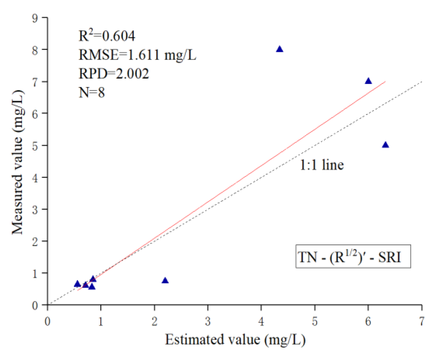
From the results of the training set, the accuracies of the two models were found to be acceptable. From the perspective of the validation set, the R2, RMSE, and RPD values of the (lg(1/R))′-SRI coupled estimation model were 0.613, 1.798 mg/L, and 1.793, respectively. Similarly, the R2, RMSE, and RPD values of the (R1/2)′-SRI coupled estimation model were 0.604, 1.6 mg/L, and 2.002, respectively. Comparing the two estimation models, it was found that the (R1/2)′-SRI model had higher accuracy, considering that while their R2 values were basically the same, their RMSE values were lower and their RPD values were higher (Figure 7 and Table 7).
Compared with the model constructed by spectral transformation or the spectral index, the PSO-SVM estimation model based on the (R1/2)′-SRI coupled form was more robust and its powers of inversion and prediction were clearly improved. Based on these positive results, we concluded that the coupling form was suitable for the quantitative estimation and prediction of total nitrogen concentration of surface water in arid areas.
4. Discussion
4.1. Theoretical Basis
The material composition of surface water determines its spectral characteristics, and differences in the surface water concentrations often result in significant differences in reflectivity in particular bands [39,40], which is the theoretical basis for inversion of water components by spectral reflectance. To study the surface water nitrogen concentration, both direct and indirect methods confirm the feasibility of using hyperspectral data to estimate surface water quality indicators [41,42]. Furthermore, in this paper, the cluster analysis method was used to make the training set and verification set more representative, which is also a powerful measure to improve the generality of the estimation model. When a small sample is used, the PSO-SVM quantitative estimation model based on a sensitive band is applicable, consistent with Nagra [43]. In addition, the representative water samples were selected to have the lowest reflectivity, ensuring estimation accuracy for high reflectivity water samples.
In the literature, the PSO-SVM estimation model is known to be suitable for small samples [44], but the definition of small samples is not clear at present. Hence, we speculate that it may be a relative concept. Although the number of samples in this paper was only 32 (24 training sets and 8 verification sets), it achieved good results in the prediction of total nitrogen concentration. Our results indicate that a sample size of 32 is suitable for the PSO-SVM model. In addition, there were 14 samples of low concentration, 8 samples of medium concentration, and 10 samples of high concentration in this study, which shows that the concentration of selected samples has good continuity. As for the training set and verification set, we randomly selected them from the three levels according to the proportion of 7:4:5, which ensured the rationality of sample selection. Based on the above theoretical basis, the results of this study are scientifically acceptable.
4.2. Selection of Sensitive Bands
The high resolution and narrow bands of hyperspectral data result in a high data dimension, making much information redundant and making some bands noisy, increasing the need for data preprocessing [45], so it is particularly important to select appropriate dimension reduction methods to quantitatively estimate water quality indicators. Sensitive band selection is one of the main widely used dimensionality reduction methods [46], and its mechanism is to highlight the relevant main signal through a series of preprocessing steps and to weaken or shield the secondary signal. In general, sensitive band of photosensitive substances in surface water is easy to extract, but this research’s object was total nitrogen in water, which is a non-photosensitive substance. Therefore, some measures had to be taken to search the sensitive band related to total nitrogen. Upon careful study it was found that the sensitive bands selected in this paper were concentrated around 680 nm, 850 nm, and 940 nm, and this is basically consistent with the studies of Schalles [47] and Yu [48].
It can be seen from Figure 2 that the spectral reflectance around these bands has different degrees of absorption, which may be caused by optically active variables in surface water. Coincidentally, Chen [49] and Li [50] proved that the total nitrogen concentration had a high correlation with chlorophyll-a, colored dissolved substances and total suspended solids, and they are all optically active variables. As for the method of selecting a sensitive band, it was found to be reliable to establish a model for quantitative estimation of total nitrogen concentration in surface water by means of spectral transformation and spectral index, similar to the methods of Zhao [51]. In particular, this paper attempted to establish a hyperspectral matrix coefficient map by coupling spectral transformation and the spectral index to screen sensitive bands. Sensitive bands are easy to identify, and the band information is rich (Figure 6). The method can be understood as two-dimensional superposition of two sensitive bands, which can better highlight the sensitive bands related to the total nitrogen concentration.
4.3. Advantage of Coupling Model
The correlation coefficient of (R1/2)′-SRI in Table 6 is smaller than that of other coupling forms, but the final evaluation index of total nitrogen concentration estimation was better than that of other coupling forms, which may be caused by different degree of over fitting phenomenon in the model estimation process under other coupling forms.
In order to intuitively show the advantages of total nitrogen concentration estimation in coupling form, we compared the optimal evaluation indices in single and coupling forms (Table 8). In the specific implementation process, we took the coupling form as the standard and used the difference between the single form evaluation index and the coupling form evaluation index to reflect the advantages of the coupling form. It can be seen from Table 8 that the optimal evaluation indices in the spectral transformation situation were all worse than those in the coupling form, while R2 in the optimal evaluation indices in the spectral index was 0.117 larger than that in the coupling form, but its RMSE was 2.9 larger than that in the latter, and RPD was 1.287 smaller than that in the latter, which shows that the estimation model error under the spectral index was large and the robustness was poor. Therefore, we know that the reliability of the coupling model was higher.
In order to further illustrate the advantages of the coupling mode in selecting sensitive band, we tested the difference of evaluation indices in the testing set. This study was based on the hyperspectral sensitive band to estimate the total nitrogen concentration, so we chose the sensitive band with high correlation with the measured total nitrogen concentration to carry out the difference study. Among them, the selection mode of sensitive band in single form included spectral transformation and spectral index (Table 3 and Table 4); the selection mode of sensitive band in coupling form is shown in Table 6. Then we defined single forms as the first group and coupling forms as the second group. Through the normal test, the authors found that R2 and RPD satisfied the normal distribution except RMSE. Therefore, independent sample t-test was used to detect the difference of R2 and RPD between the two groups, and independent sample nonparametric test was used to detect the difference of RMSE. The results are shown in Table 9.
It can be seen from Table 9 that the t-test result of R2 was greater than 0.05, indicating that there was no significant difference in R2 between the two groups; similarly, the t-test result of RPD was 0.024, and the non-parametric test result of RMSE was only 0.03, indicating that there is significant difference in RPD and RMSE. The average values of the first and second groups of evaluation indicators also supported the above views. In addition, R2 and RPD of the second group were 0.057 and 0.524 larger than that of the first group, and RMSE was 0.964 smaller than that of the first group. Therefore, combined with all the above analysis, we conclude that the PSO-SVM model constructed by the sensitive band optimized by coupling form has stronger prediction ability.
4.4. Deficiencies and Prospects
This study only considered one year’s field data rather than a long time series, possibly explaining the relatively low inversion accuracy of this model [52]. Whether the model selected in this study is suitable for other regions, as well as the efficacy of using other data sources to estimate the total nitrogen concentration in surface water, need to be further verified [53]. Eventually, the inversion model presented in this study was based on surface water samples, and the accuracy of models based on water samples from the whole water column remains to be studied.
5. Conclusions
In this study, a new strategy was selected to improve the hyperspectral estimation of total nitrogen concentration in surface water. The main conclusions are as follows:
- (1)
- After determination, the nitrogen concentration of all samples was quite variable, the coefficient of variation was 83.12%, and the concentration in the lower reaches was roughly higher than that in the upper reaches.
- (2)
- Through correlation analysis of the hyperspectral reflectance value and the measured nitrogen concentration under spectral transformation, the spectral index and their coupling forms, it was found that the bands near 680, 850, and 940 nm can be used as the sensitive bands for the inversion of the total nitrogen concentration in surface water in arid areas.
- (3)
- After optimization, in the estimation model based on the sensitive bands, the model based on the coupling form of (R1/2)′-SRI had the highest accuracy, followed by the accuracy of the model based on (R1/2)′ spectral transformation and that of the model based on the SDI spectral index.
In summary, compared with the estimation model based on spectral transformation or the spectral index alone, the estimation model based on the coupled form had the greatest accuracy, potentially providing a new method for improving the efficiency and accuracy of surface water nitrogen concentration monitoring in arid regions.
Author Contributions
Conceptualization, C.L. and F.Z.; methodology, C.L.; software, X.G.; validation, C.L. X.Z. and F.Z.; formal analysis, C.L.; investigation, C.L. and Y.Q.; resources, F.Z.; data curation, C.L.; writing—original draft preparation, C.L.; writing—review and editing, N.w.C.; visualization, C.L. and X.Z.; supervision, F.Z.; project administration, F.Z.; funding acquisition, F.Z. All authors have read and agreed to the published version of the manuscript.
Funding
This research was funded by the National Natural Science Foundation of China (U1603241), the National Natural Science Foundation of China (Xinjiang Local Outstanding Young Talent Cultivation) (Grant No. U1503302), the Tianshan Talent Project of Xinjiang Uygur Autonomous Region (400070010209), and the Group supporting projects for study abroad sent by the People’s Government of the Autonomous Region (Grant No. L06).
Acknowledgments
Sincere thanks are also extended to the teachers and students of the Key Laboratory of Oasis Ecology Department of Xinjiang University for their support and help. Furthermore, I would like to express my special thanks to Ngai Wen Chan, a professor at the University of Sains in Malaysia, for his valuable suggestions on punctuation, typographical errors, grammar, etc. Finally, the authors would like to thank the reviewers and editors for providing helpful suggestions to improve this manuscript.
Conflicts of Interest
The authors declare no conflict of interest.
References
- Wu, Y.Z.; Wu, Y.Y.; Gu, B.J. Urban rivers as hotspots of regional nitrogen pollution. Environ. Pollut. 2015, 205, 139–144. [Google Scholar]
- Bricker, S.B.; Rice, K.C.; Bricker, O.P. From Headwaters to Coast: Influence of Human Activities on Water Quality of the Potomac River Estuary. Aquat. Geochem. 2014, 20, 291–323. [Google Scholar] [CrossRef]
- Räike, A.; Pietiläinen, O.; Rekolainen, S.; Kauppila, P.; Pitkanen, H.; Niemi, J.; Raateland, A.; Vuorenmaa, J. Trends of phosphorus, nitrogen and chlorophyll a concentrations in Finnish rivers and lakes in 1975–2000. Sci. Total Environ. 2003, 310, 47–59. [Google Scholar] [CrossRef]
- Biello, D. Fertilizer Runoff Overwhelms Streams and Rivers--Creating Vast “Dead Zones”. Sci. Am. 14 March 2008. Available online: https://www.scientificamerican.com/article/fertilizer-runoff-overwhelms-streams/ (accessed on 20 June 2020).
- Smith, V.H.; Tilman, G.D.; Nekola, J.C. Eutrophication: Impacts of excess nutrient inputs on freshwater, marine, and terrestrial ecosystems. Environ. Pollut. 1999, 100, 179–196. [Google Scholar] [CrossRef]
- Sun, X. Yangtze and Pearl River Estuaries Now ‘Dead Zones’. China Daily. Available online: http://www.chinadaily.com.cn/china/2006-10/20/content_712573.htm (accessed on 7 April 2020).
- Hilborn, E.D.; Roberts, V.A.; Backer, L.; Deconno, E.; Egan, J.S.; Hyde, J.B.; Nicholas, D.; Wiegert, E.; Billing, L.; Diorio, M.; et al. Algal bloom-associated disease outbreaks among users of freshwater lakes--United States, 2009–2010. MMWR-Morb. Mortal. Wkly. Rep. 2014, 63, 11–15. [Google Scholar] [PubMed]
- Wang, X.; Zhang, F.; Kung, H.T.; Ghulam, A.; Trumbo, A.L.; Yuan, J. Evaluation and estimation of surface water quality in an arid region based on EEM-PARAFAC and 3D fluorescence spectral index: A case study of the Ebinur Lake Watershed, China. Catena 2017, 155, 62–74. [Google Scholar] [CrossRef]
- Mohammad, H.G.; Assefa, M.M.; Lakshmi, R. A Comprehensive Review on Water Quality Parameters Estimation Using Remote Sensing Techniques. Sensors 2016, 16, 1298. [Google Scholar]
- Tasistro, A.S.; Shaaban, S.; Kissel, D.E.; Vendrell, P.F. Near-Infrared Reflectance Spectroscopy for the Analysis of Water and Total Nitrogen Concentrations in Poultry Litter. Commun. Soil Sci. Plant Anal. 2003, 34, 1367–1379. [Google Scholar] [CrossRef]
- Liu, J.M.; Zhang, Y.J.; Yuan, D.; Song, X.Y. Empirical Estimation of Total Nitrogen and Total Phosphorus Concentration of Urban Water Bodies in China Using High Resolution IKONOS Multispectral Imagery. Water 2015, 7, 6551–6573. [Google Scholar] [CrossRef] [Green Version]
- Amiri, B.J.; Nakane, K. Comparative Prediction of Stream Water Total Nitrogen from Land Cover Using Artificial Neural Network and Multiple Linear Regression Approaches. Pol. J. Environ. Stud. 2009, 18, 151–160. [Google Scholar]
- Liu, H.; Gong, Z.N.; Zhao, W.J. Estimating total nitrogen concentration in reclaimed water based on hyperspectral reflectance information from emergent plants: A case study of Mencheng Lake Wetland Park in Beijing. Chin. J. Appl. Ecol. 2014, 25, 3609–3618. (In Chinese) [Google Scholar]
- Pan, B.L.; Yi, W.N.; Wang, X.H.; Qin, H.P.; Wang, J.C.; Qiao, Y.L. Inversion of the Lake Total Nitrogen Concentration by Multiple Regression Kriging Model Based on Hyperspectral Data of HJ-1A. Spectrosc. Spectr. Anal. 2011, 31, 1884–1888. (In Chinese) [Google Scholar]
- Pan, B.Z.; Wang, H.J.; Liang, X.M.; Wang, H.Z. Factors influencing chlorophyll a concentration in the yangtze-connected lakes. FRESENIUS Environ. Bull. 2009, 18, 1894–1900. [Google Scholar]
- Jia, F. The feasibility research for detecting the nitrogen concentration in sewage quickly and continuously with NIPGA. J. Northeast Norm. Univ. 2013, 45, 88–90. (In Chinese) [Google Scholar]
- Hook, A.M.; Yeakley, J.A. Stormflow Dynamics of Dissolved Organic Carbon and Total Dissolved Nitrogen in a Small Urban Watershed. Biogeochemistry 2005, 75, 409–431. [Google Scholar] [CrossRef]
- Yamazaki, Y.; Muneoka, T.; Wakou, S.; Kimura, M.; Tsuji, O. Evaluation of the Ion Components for the Estimation of Total Nitrogen Concentration in River Water based on Electrical Conductivity. J. Drugs Dermatol. JDD 2014, 13, 1491–1493. [Google Scholar]
- Chang, N.B.; Imen, S.; Vannah, B. Remote Sensing for Monitoring Surface Water Quality Status and Ecosystem State in Relation to the Nutrient Cycle: A 40-Year Perspective. Crit. Rev. Environ. Sci. Technol. 2015, 45, 101–166. [Google Scholar] [CrossRef]
- Gao, Q.; Chen, S.; Kimirei, I.A.; Zhang, L.; Mgana, H.; Mziray, P.; Wang, Z.; Yu, C.; Shen, Q.S. Wet deposition of atmospheric nitrogen contributes to nitrogen loading in the surface waters of Lake Tanganyika, East Africa: A case study of the Kigoma region. Environ. Sci. Pollut. Res. 2018, 25, 1–15. [Google Scholar] [CrossRef]
- Song, G.Q.; Yin, M.; Zhang, W.D.; Jiang, B. Determination of concentration and fluxes of total nitrogen in river entries of Danjiangkou Reservoir. Environ. Sci. Technol. 2009, 32, 135–137. [Google Scholar]
- Medjahed, S.A.; Ouali, M. Band selection based on optimization approach for hyperspectral image classification. Egypt. J. Remote Sens. Space Sci. 2018, 21, 413–418. [Google Scholar] [CrossRef]
- Sun, W.; Du, Q. Hyperspectral Band Selection: A Review. IEEE Geosci. Remote. Sens. Mag. 2020, 2, 118–139. [Google Scholar] [CrossRef]
- Lorenzo, P.R.; Tulczyjew, L.; Marcinkiewicz, M.; Nalepa, J. Hyperspectral Band Selection Using Attention-Based Convolutional Neural Networks. IEEE Access 2020, 8, 42384–42403. [Google Scholar] [CrossRef]
- Wang, X.; Zhang, F.; Hsiang-te, K.; Verner, C.J. New methods for improving the remote sensing estimation of soil organic matter concentration (SOMC) in the Ebinur Lake Wetland National Nature Reserve (ELWNNR) in northwest China. Remote Sens. Environ. 2018, 218, 104–118. [Google Scholar] [CrossRef]
- Zhu, S.; Zhang, F.; Zhang, Z.; Kung, H.; Yushanjiang, A. Hydrogen and Oxygen Isotope Composition and Water Quality Evaluation for Different Water Bodies in the Ebinur Lake Watershed, Northwestern China. Water 2019, 11, 2067. [Google Scholar] [CrossRef] [Green Version]
- Gentle, B.S.; Ellis, P.S.; Grace, M.R.; Mckelvie, I.D. Flow analysis methods for the direct ultra-violet spectrophotometric measurement of nitrate and total nitrogen in freshwaters. Anal. Chim. Acta 2011, 704, 116–122. [Google Scholar] [CrossRef] [PubMed]
- Curcio, D.; Ciraolo, G.; D’Asaro, F.; Minacapilli, M. Prediction of Soil Texture Distributions Using VNIR-SWIR Reflectance Spectroscopy. Procedia Environ. Sci. 2013, 19, 494–503. [Google Scholar] [CrossRef] [Green Version]
- Rakshit, S.; Ghosh, A.; Shankar, B.U. Fast mean filtering technique (FMFT). Pattern Recognit. 2007, 40, 890–897. [Google Scholar] [CrossRef]
- Gitelson, A.A.; Kondratyev, K.Y. Optical models of mesotrophic and eutrophic water bodies. Int. J. Remote Sens. 1991, 12, 373–385. [Google Scholar] [CrossRef]
- Gons, H.J.; Auer, M.T.; Effler, S.W. MERIS satellite chlorophyll mapping of oligotrophic and eutrophic waters in the Laurentian Great Lakes. Remote Sens. Environ. 2008, 112, 098–4106. [Google Scholar] [CrossRef]
- Hong, Y.; Chen, S.; Zhang, Y.; Chen, Y.Y.; Yu, L.; Liu, Y.F.; Liu, Y.L.; Cheng, H.; Liu, Y. Rapid identification of soil organic matter level via visible and near-infrared spectroscopy: Effects of two-dimensional correlation coefficient and extreme learning machine. Sci. Total Environ. 2018, 644, 1232–1243. [Google Scholar] [CrossRef]
- Nawar, S.; Buddenbaum, H.; Hill, J. Estimation of soil salinity using three quantitative methods based on visible and near-infrared reflectance spectroscopy: A case study from Egypt. Arab. J. Geosci. 2015, 8, 5127–5140. [Google Scholar] [CrossRef]
- Meng, L.; Zhou, S.; Zhang, H.; Bi, X.L. Estimating soil salinity in different landscapes of the Yellow River Delta through Landsat OLI/TIRS and ETM+ Data. J. Coast. Conserv. 2016, 20, 271–279. [Google Scholar] [CrossRef]
- Huang, C.L.; Dun, J.F. A distributed PSO–SVM hybrid system with feature selection and parameter optimization. Appl. Soft Comput. 2008, 8, 1381–1391. [Google Scholar] [CrossRef]
- Nocita, M.; Stevens, A.; Noon, C.; van Wesemael, B. Prediction of soil organic carbon for different levels of soil moisture using Vis-NIR spectroscopy. Geoderma 2013, 199, 37–42. [Google Scholar] [CrossRef]
- Qi, H.; Paz-Kagan, T.; Karnieli, A.; Jin, X.; Li, S. Evaluating calibration methods for predicting soil available nutrients using hyperspectral VNIR data. Soil Tillage Res. 2018, 175, 267–275. [Google Scholar] [CrossRef]
- Wang, X.; Zhang, F. Effects of land use/cover on surface water pollution based on remote sensing and 3D-EEM fluorescence data in the Jinghe Oasis. Sci. Rep. 2018, 8, 13099. [Google Scholar] [CrossRef]
- Ma, R.; Tang, J.; Dai, J.; Zhang, Y.L.; Song, Q. Absorption and scattering properties of water body in Taihu Lake, China: Absorption. Int. J. Remote Sens. 2006, 27, 4277–4304. [Google Scholar] [CrossRef]
- Nakariyakul, S. Fast spatial averaging: An efficient algorithm for 2D mean filtering. J. Supercomput. 2013, 65, 262–273. [Google Scholar] [CrossRef]
- Fan, C. Spectral Analysis of Water Reflectance for Hyperspectral Remote Sensing of Water Quailty in Estuarine Water. J. Geosci. Environ. Prot. 2014, 2, 19–27. [Google Scholar] [CrossRef]
- Tan, J.; Cherkauer, K.A.; Chaubey, I. Using hyperspectral data to quantify water-quality parameters in the Wabash River and its tributaries, Indiana. Int. J. Remote Sens. 2015, 36, 5466–5484. [Google Scholar] [CrossRef]
- Nagra, A.A.; Han, F.; Ling, Q.H.; Mehta, S. An Improved Hybrid Method Combining Gravitational Search Algorithm with Dynamic Multi Swarm Particle Swarm Optimization. IEEE Access 2019, 7, 50388–50399. [Google Scholar] [CrossRef]
- García Nieto, P.J.; García-Gonzalo, E.; Alonso Fernández, J.R.; Muñizb, C.D. Hybrid PSO–SVM-based method for long-term forecasting of turbidity in the Nalón river basin: A case study in Northern Spain. Ecol. Eng. 2014, 73, 192–200. [Google Scholar] [CrossRef]
- Hasanlou, M.; Samadzadegan, F. Comparative Study of Intrinsic Dimensionality Estimation and Dimension Reduction Techniques on Hyperspectral Images Using K-NN Classifier. IEEE Geosci. Remote Sens. Lett. 2012, 9, 1046–1050. [Google Scholar] [CrossRef]
- Zhao, W.; Du, S. Spectral–spatial feature extraction for hyperspectral image classification: A dimension reduction and deep learning approach. IEEE Trans. Geosci. Remote Sens. 2016, 54, 4544–4554. [Google Scholar] [CrossRef]
- Schalles, J.F.; Gitelson, A.A.; Yacobi, Y.Z.; Kroenke, A.E. Estimation of chlorophyll a from time series measurements of high spectral resolution reflectance in an eutrophic lake. J. Phycol. 2002, 34, 383–390. [Google Scholar] [CrossRef]
- Yu, X.; Yi, H.; Liu, X.; Wang, Y.B.; Liu, X.; Zhang, H. Remote-sensing estimation of dissolved inorganic nitrogen concentration in the Bohai Sea using band combinations derived from MODIS data. Int. J. Remote Sens. 2016, 37, 327–340. [Google Scholar] [CrossRef]
- Chen, S.; Han, L.; Chen, X.; Li, D.; Sun, L.; Li, Y. Estimating wide range Total Suspended Solids concentrations from MODIS 250-m imageries: An improved method. ISPRS J. Photogramm. Remote Sens. 2015, 99, 58–69. [Google Scholar] [CrossRef]
- Li, K.; Xiao, P. Temporal and Spatial Distribution of Chlorophyll-A Concentration and Its Relationships with TN, TP Concentrations in Lake Chaohu. J. Biol. 2011, 28, 53–56. (In Chinese) [Google Scholar]
- Zhao, K.; Valle, D.; Popescu, S.; Zhang, X.S.; Mallick, B.K. Hyperspectral remote sensing of plant biochemistry using Bayesian model averaging with variable and band selection. Remote Sens. Environ. 2013, 132, 102–119. [Google Scholar] [CrossRef]
- Liang, Y.; Joachim, R.; Van, B.B.M.; Ouboter, M.; Vlugt, C.V.D.; Broers, H.P. Groundwater impacts on surface water quality and nutrient loads in lowland polder catchments: Monitoring the greater Amsterdam area. Hydrol. Earth Syst. Sci. 2018, 22, 487–508. [Google Scholar]
- Hao, Z.; Gao, Y.; Yang, T.; Tian, J. Atmospheric wet deposition of nitrogen in a subtropical watershed in China: Characteristics of and impacts on surface water quality. Environ. Sci. Pollut. Res. 2017, 24, 8489–8503. [Google Scholar] [CrossRef] [PubMed]
Figure 1.
(a) A satellite image from Landsat 8 of the study area; (b) location map of the study area; (c) landscape of water quality in the upper reaches of Jinghe River; and (d) landscape of water quality in the lower reaches of Bortala River (photographed (c,d) by Changjiang Liu; map of (a,b) by ArcGIS10.3.1 (http://www.esri.com/software/arcgis)).

Figure 2.
Spectrum curve of water samples and variation of the nitrogen concentration.

Figure 3.
Search for the hyperspectral sensitive band under the spectral transformation.


Figure 4.
Search for the hyperspectral sensitive band under the spectral index.

Figure 5.
Estimation results for the total nitrogen concentration using a PSO-SVM model (the triangle in the figure represents the testing sample).
Figure 5.
Estimation results for the total nitrogen concentration using a PSO-SVM model (the triangle in the figure represents the testing sample).

Figure 6.
Search for the hyperspectral sensitive band with the combination of spectral transformation and the spectral index.
Figure 6.
Search for the hyperspectral sensitive band with the combination of spectral transformation and the spectral index.


Figure 7.
The best accuracy of PSO-SVM estimation model (the triangle in the figure represents the testing sample).
Figure 7.
The best accuracy of PSO-SVM estimation model (the triangle in the figure represents the testing sample).


Table 1.
Spectral transformation forms.
| Number | Spectral Transformation Method | Abbreviation |
|---|---|---|
| 1 | First derivative | R′ |
| 2 | Second derivative | R′′ |
| 3 | Square root of R | R1/2 |
| 4 | First derivative of R square root | (R1/2)′ |
| 5 | Second derivative of R square root | (R1/2)′′ |
| 6 | Inverse of R | 1/R |
| 7 | First derivative of inverse | (1/R)′ |
| 8 | Second derivative of inverse | (1/R)” |
| 9 | Logarithm of R | lgR |
| 10 | First derivative of logarithm | (lgR)′ |
| 11 | Second derivative of logarithm | (lgR)′′ |
| 12 | Logarithm of 1/R | lg(1/R) |
| 13 | First derivative of 1/R logarithm | (lg(1/R))′ |
| 14 | Second derivative of 1/R logarithm | (lg(1/R))′′ |
Note: The original spectral reflectance is recorded as R.
Table 2.
Constructed spectral index.
| Spectral Index | Calculation Formula | Reference |
|---|---|---|
| SDI | Rj − Ri | [33] |
| SRI | Rj /Ri | |
| SNDI | Rj − Ri /Rj + Ri | [34] |
Note: Ri and Rj are the original reflectivity of any two bands in the band range.
Table 3.
Selection of sensitive bands and correlation coefficients under the different spectral transformations.
Table 3.
Selection of sensitive bands and correlation coefficients under the different spectral transformations.
| Spectral Transformation | Sensitive Bands (nm) | Correlation Coefficient |
|---|---|---|
| (R1/2)′ | 665, 688 | −0.72, 0.80 |
| (R1/2)′′ | 659, 723 | −0.61, −0.59 |
| (1/R)′ | 660, 762 | 0.68, −0.67 |
| (1/R)′′ | 761, 766 | −0.55, 0.57 |
| (lgR)′ | 657, 691 | −0.70, 0.78 |
| (lgR)′′ | 659, 767 | −0.57, −0.60 |
| (lg(1/R))′ | 662, 689 | 0.71, −0.79 |
| (lg(1/R))′′ | 658, 766 | 0.54, 0.59 |
Table 4.
Sensitive band selection and correlation coefficients based on the spectral indices.
| Spectral Indices | Sensitive Bands Combination (nm) | Correlation Coefficient |
|---|---|---|
| SDI | (693, 683) | 0.71 |
| SNDI | (693, 687) | 0.69 |
| SRI | (693, 687) | 0.69 |
Table 5.
Estimation accuracy of the optimal models based on spectral transformation and the spectral index.
Table 5.
Estimation accuracy of the optimal models based on spectral transformation and the spectral index.
| Sensitive Band Optimization Method | Training Set | Testing Set | ||||
|---|---|---|---|---|---|---|
| R2 | RMSE (mg/L) | RPD | R2 | RMSE (mg/L) | RPD | |
| (R1/2)′ | 0.814 | 0.899 | 3.260 | 0.562 | 1.516 | 2.126 |
| (lg(1/R))′ | 0.820 | 0.622 | 4.710 | 0.576 | 1.624 | 1.985 |
| SDI | 0.682 | 0.930 | 3.150 | 0.721 | 4.511 | 0.715 |
Table 6.
Sensitive band combination and correlation coefficients for the combination of spectral transformation and the spectral index.
Table 6.
Sensitive band combination and correlation coefficients for the combination of spectral transformation and the spectral index.
| Coupling Forms | Sensitive Bands Combination (nm) | Correlation Coefficient |
|---|---|---|
| (R1/2)′-SDI | (691, 661) | 0.76 |
| (R1/2)′-SNDI | (690, 388) | 0.65 |
| (R1/2)′-SRI | (848, 687) | 0.62 |
| (lg(1/R))′-SDI | (690, 661) | 0.73 |
| (lg(1/R))′-SNDI | (687, 383) | 0.65 |
| (lg(1/R))′-SRI | (939, 840) | 0.72 |
| (lgR)′-SDI | (691, 661) | 0.71 |
| (lgR)′-SNDI | (690, 388) | 0.69 |
| (lgR)′-SRI | (848, 688) | 0.69 |
Table 7.
Estimation accuracy based on spectral transformation and spectral index coupling models.
| Coupling Forms | Training Set | Testing Set | ||||
|---|---|---|---|---|---|---|
| R2 | RMSE (mg/L) | RPD | R2 | RMSE (mg/L) | RPD | |
| (R1/2)′-SRI | 0.653 | 0.97 | 3.022 | 0.604 | 1.611 | 2.002 |
| (lg(1/R))′-SRI | 0.751 | 0.948 | 3.094 | 0.613 | 1.798 | 1.793 |
Table 8.
Reliability comparison of optimal evaluation indexes in single and coupling forms.
| Evaluation Indices | Coupling Form | Spectral Transformation | Spectral Index | ||
|---|---|---|---|---|---|
| (R1/2)′-SRI | (lg(1/R))′ | Difference | SDI | Difference | |
| R2 | 0.604 | 0.576 | −0.028 ↓ | 0.721 | 0.117 ↑ |
| RMSE | 1.611 | 1.624 | 0.013 ↓ | 4.511 | 2.9 ↓ |
| RPD | 2.002 | 1.985 | −0.017 ↓ | 0.715 | −1.287 ↓ |
Notes: ↓ means worse than coupling form, ↑ means better than coupling form.
Table 9.
Difference test of evaluation indices in single and coupling forms.
| Evaluation Indices | Testing Method | Significance | Result | Average Value (First Group) | Average Value (Second Group) |
|---|---|---|---|---|---|
| R2 | t-test | 0.542 | No significant difference | 0.357 | 0.414 |
| RPD | 0.023 | Significant difference | 1.253 | 1.777 | |
| RMSE | Nonparametric statistical test (Mann–Whitney) | 0.030 | Significant difference | 2.949 | 1.985 |
Note: If the significance is greater than 0.05, there is no significant difference between the two groups; if the significance is less than 0.05, there is significant difference.
© 2020 by the authors. Licensee MDPI, Basel, Switzerland. This article is an open access article distributed under the terms and conditions of the Creative Commons Attribution (CC BY) license (http://creativecommons.org/licenses/by/4.0/).
Share and Cite
MDPI and ACS Style
Liu, C.; Zhang, F.; Ge, X.; Zhang, X.; Chan, N.w.; Qi, Y. Measurement of Total Nitrogen Concentration in Surface Water Using Hyperspectral Band Observation Method. Water 2020, 12, 1842. https://doi.org/10.3390/w12071842
AMA Style
Liu C, Zhang F, Ge X, Zhang X, Chan Nw, Qi Y. Measurement of Total Nitrogen Concentration in Surface Water Using Hyperspectral Band Observation Method. Water. 2020; 12(7):1842. https://doi.org/10.3390/w12071842
Chicago/Turabian StyleLiu, Changjiang, Fei Zhang, Xiangyu Ge, Xianlong Zhang, Ngai weng Chan, and Yaxiao Qi. 2020. "Measurement of Total Nitrogen Concentration in Surface Water Using Hyperspectral Band Observation Method" Water 12, no. 7: 1842. https://doi.org/10.3390/w12071842
Note that from the first issue of 2016, this journal uses article numbers instead of page numbers. See further details here.