Symmetrical Rank-Three Vectorized Loading Scores Quasi-Newton for Identification of Hydrogeological Parameters and Spatiotemporal Recharges

Abstract

In a multi-layered groundwater model, achieving accurate spatiotemporal identification and solving the ill-posed problem is the vital topic for model calibration. This study proposes a symmetry rank three vectorized loading scores (SR3 VLS) quasi-Newton algorithm by modifying the Levenberg–Marquardt algorithm and importing a rank three structure from Broyden–Fletcher–Goldfarb–Shanno algorithm for identification of hydrogeological parameters and spatiotemporal recharge simultaneously. To accelerate directional convergence and approach a global optimum, this study uses a vectorized limited switchable step size in the transmissive groundwater inverse problem. The Hessian approximation rank three uses high and low-rank factor loading scores analyzed from simulated storage fluctuation between adjacent iterations for calculation and matrix correction. Two numerical experiments were designed to validate the proposing algorithm, showing the SR3 VLS quasi-Newton reduced the error percentages of the identified parameters by 1.63% and 9.65% compared to the Jacobian quasi-Newton. The proposing method is applied to the Chou-Shui River alluvial fan groundwater system in Taiwan. Results show that the simulated storage error decreased rapidly in six iterations, and has good head convergence as small as 0.11% with a root-mean-square-error (RMSE) of 0.134 m, indicating that the proposing algorithm reduces the computational cost to converge to the true solution.

1. Introduction

In arid and semi-arid areas, if there are insufficient surface water facilities to store runoff, groundwater provides an important water supply source [1]. Conjunctive use planning for surface water and groundwater plays an important role in total water resource management and can be optimized through a sound groundwater management model based on mathematical system analysis. To develop such a model, it is necessary to understand and to be able to estimate the spatiotemporal patterns of pumpage, net recharge, and hydrogeological parameters of the groundwater system, in which the associated simulation model and optimization model are mostly nonlinear. The governing equation of three-dimensional groundwater flow can be expressed as [2]

$$\frac{\partial }{\partial x}(K_{xx}\frac{\partial h}{\partial x})+\frac{\partial }{\partial y}(K_{yy}\frac{\partial h}{\partial y})+\frac{\partial }{\partial z}(K_{zz}\frac{\partial h}{\partial z})+W=S_s\frac{\partial h}{\partial t}$$

(1)

where $K_{xx}$, $K_{yy}$, and $K_{zz}$ are the hydraulic conductivities along the x, y, and z directions (LT⁻¹); $S_s$ is the specific storage of porous media (L⁻¹); h is the groundwater head (L); W is the volumetric flux per unit volume representing sources (recharge) and/or sinks (pumpage) of the groundwater system, $W>0$ for the flow into the system (T⁻¹); t is the time (T).

It can be seen from Equation (1) that before simulating groundwater flow, the spatiotemporal patterns of pumpage and recharge must be specified and the hydrogeological parameters identified. However, in previous studies, the establishment of a groundwater flow model has focused on hydrogeological parameter identification. The spatiotemporal patterns of pumpage and net recharge are mostly regarded as known [3,4,5,6,7,8,9,10,11,12,13,14,15]. If the pumpage and recharge spatiotemporal patterns are arbitrary, the calibrated model is subject to uncertainty [16]. Furthermore, previous studies on hydrogeological parameter identification are usually based on hypothetical cases, which seldom apply to large-scale complex groundwater systems.

The nonlinear programming is the traditional parameter identification method in groundwater modeling. Therein, Newton’s method is used to find the roots of first-order partial derivatives of the objective function $J^{\prime }\left({\mathsf{\eta }}^{*}\right)=0$ by constructing a parameter sequence ${\mathsf{\eta }}^k$ based on the initial guess ${\mathsf{\eta }}^0$ that converges towards some optimal value ${\mathsf{\eta }}^{*}$ with the use of the Jacobian matrix [17], which is the first-order partial derivatives of a scalar-valued model output function. Subsequently, to improve the convergence rate of parameter (decision variable) identification, the Hessian matrix, which is a square matrix of second-order partial derivatives of the objective function (or scalar field), was employed in the Gauss–Newton method [18]. The Hessian describes the local curvature of a function of many parameters; thus, the Gauss–Newton tends to search for the parameter value along a shorter and more direct path calculated from a direction compared to that of Newton’s method [19]. However, finding the inverse of the Hessian in high dimensions can be an expensive operation, which can be addressed via various factorizations or approximately using iterative methods. Moreover, computing and storing the full Hessian matrix requires the squared number of parameters in memory, which is unfeasible for high dimensional functions/models with several parameters [17]. Furthermore, if the Hessian is similar to a non-invertible matrix, the inverted Hessian can be numerically unstable, and the solution may diverge. For such situations, quasi-Newton algorithms have been developed, where an approximation for the Hessian is constructed from changes in the gradient. The most commonly used quasi-Newton algorithms are the Jacobian quasi-Newton method, Levenberg–Marquardt algorithm (LMA), and Broyden–Fletcher–Goldfarb–Shanno (BFGS) algorithm.

The Jacobian quasi-Newton often overestimates the Hessian [17]; hence, the convergence may not be guaranteed in transmissive groundwater problems, and the problem may be ill-posed. Contrarily, LMA is more robust than the Jacobian quasi-Newton due to the addition of a diagonal correction matrix; however, it tends to be slower. Furthermore, LMA converges to the global minimum only if the initial estimate is already close to the global minimum [20]. The BFGS algorithm is not used for solving constrained nonlinear optimization. Moreover, Newton’s method and the BFGS algorithm do not guarantee convergence unless the function has a quadratic Taylor expansion near an optimum position [21]. A key reason leading to the above-mentioned challenges is the scalar nature of the step size in the Jacobian quasi-Newton, the Marquardt damping factor in LMA, and the secant scale factor in BFGS.

In Newton’s method and the quasi-Newton algorithm for nonlinear optimization, the line search algorithm in the calculated direction $d^k$ is used to find the next solution ${\mathsf{\eta }}^{k+1}$ by minimizing the corresponding objective function, $J=f\left({\mathsf{\eta }}^k+{\alpha }^k·d^k\right)$, over the scalar step size ${\alpha }^k>0$. The line search strategy is one of two basic iterative approaches to find a locally optimal solution for scalar step size by minimizing the objective function. The other approach is the trust region. The line search approach first determines a gradient descent direction along which the objective function $J$ will be reduced and subsequently computes a step size that determines how far the vector of parameters $\mathsf{\eta }$ should move along that direction. In the commonly used direct search double false position method, the minimum must be bracketed in an interval; therefore, it always converges and is capable of targeting more difficult problems [22]. Modern versions of the false position method employ systematic methods of choosing new test values and are concerned with approximation speed. If a computer program needs to repeatedly solve equations during its run, faster methods with significant time savings are preferred. If the scalar step size expands to the vectorized limited step size and simultaneously modifies the direction $d^k$ for better Hessian approximation, to accelerate shrinking between the step size bracketed intervals, initial interval selection and systematic acceleration approach are key for efficient optimization.

Recently, a few studies used advanced approaches for the identification of hydrogeological parameters or source/sink to satisfy objective convergence conditions. However, few studies have worked on a modified quasi-Newton algorithm for converging to the parameter’s true solution and reducing the computational cost. Tung and Chou [23] integrated pattern classification and Tabu Search to optimize zonation and associated average groundwater pumping rates. Tsai and Yeh [24] used a genetic algorithm embedded with a Bayesian estimator to solve the transmissivity structure identification problem in a two-dimensional confined aquifer. Cheng et al. [25] developed a nudging data assimilation algorithm for estimating unknown pumping from private wells in an aquifer system. Liu et al. [26] combined the adjoint state and gradient search methods to simultaneously estimate the storage coefficient, transmissivity, initial condition, and boundary conditions. Liu and Hsu [27] used independent component analysis to identify the local pumping and recharging source. Liu et al. [28] used independent component analysis to identify the main pumping type characteristics and estimate the pumping type quantities with a calibrated groundwater simulation model. To enhance the identified accuracy of multiple parameters, this study modifies an iterative quasi-Newton algorithm using a vectorized switchable step size to simultaneously identify hydrogeological parameters and spatiotemporal patterns of pumpage and recharge in a multi-layered groundwater system.

Groundwater head (storage) hydrograph time–frequency analysis has been used to estimate recharge with reasonable results [29,30,31,32,33,34,35]. However, the control volume of the hydrograph fluctuation analysis uses a lumped parameter approach; thus, it can only estimate pumpage or recharge temporally and not spatially. In most previous studies, groundwater recharge is limited to rainfall and river recharge, and recharge across the boundary has received less attention. Furthermore, singular value decomposition (SVD) can be used to identify the factors and the corresponding magnitudes that cause the groundwater flow fluctuation. Moon et al. [33] applied SVD to explore the relationship between groundwater head fluctuation and recharge, and Yu and Chu [36] analyzed the principal factors affecting the groundwater head using an empirical orthogonal function (EOF). However, previous large-scale groundwater modeling studies have seldom used SVD-calculated loadings and scores to approximate or correct the Hessian matrix.

Thus far, very few studies have investigated large systems conditioned by actual data. This study proposes a symmetry rank three vectorized loading scores (SR3 VLS) quasi-Newton algorithm by modifying the Levenberg–Marquardt algorithm and importing a rank three structure from the Broyden–Fletcher–Goldfarb–Shanno (BFGS) algorithm to solve the constrained hydrogeological parameter identification and recharge spatiotemporal patterns simultaneously in a large-scale multi-layered groundwater model. To accelerate convergence, approach a global optimum, and achieve a well-posed problem, this study uses a vectorized limited switchable step size in the transmissive groundwater inverse problem. Accordingly, to achieve the Hessian approximation, solve nonlinear ill-posed problems, and detect the area of global minimum, a rank three structure with high- and low-rank factor loading scores analyzed from the simulated storage fluctuation between two adjacent iterations is used to calculate the correction matrix for the Hessian. The proposing methodology is verified using numerical experiments and is applied in a complex practical groundwater system.

2. Methodology

This study designs the depictions of the Section Methodology composing of five sub-sections. Section 2.1 shows the proposing optimization model for model calibration in a multi-layer groundwater system. Section 2.2 expresses the proposing SR3 VLS quasi-Newton algorithm by modifying the notable Levenberg–Marquardt algorithm and importing a rank three structure from the BFGS algorithm for solving the constrained identification of hydrogeological parameters and spatiotemporal patterns of recharges simultaneously in a large-scale transmissive groundwater model. Section 2.3 expresses the vectorized multi-order derivative exact double false position bracketing using SVD-related rank and depth modified from the traditional scalar line search. Section 2.4 depicts the procedures of the methodology. Section 2.5 expresses the visualized SVD of the change in storage between k^th and (k − 1)^th iteration for Hessian approximation.

2.1. Proposing Optimization Model for Model Calibration in a Multi-Layer Groundwater System

Traditionally, for model calibration purposes, a set of the hydrogeological parameters or source/sink patterns ($\mathsf{\eta }$) are optimized from a limited number of observations ($h_{t,x,y}^{\mathrm{obs}}$). If the classical least-squares error (LSE) is used to represent the output simulated groundwater head error, the objective function can be expressed as the minimization problem in Equation (2a) [37]. In this study, the order differs substantially between the storage coefficient in confined aquifers and the specific yield in unconfined aquifers, which are the dominant independent groundwater head fluctuation variables, thus, this study devises the LSE of the simulated and observed storage hydrograph ($q_{t_{\mathrm{s}},s_f,f}^{\mathrm{sim}}$ and $q_{t_{\mathrm{s}},s_f,f}^{\mathrm{obs}}$) as the objective function to optimize the parameter vector $\mathsf{\eta }$. The proposing minimized objective function is expressed in Equation (2b):

$$\underset{\mathsf{\eta }}{Min}\begin{array}{cc}& J\left(\mathsf{\eta }\right)\end{array}={\left[h_{t,x,y}^{\mathrm{sim}}\left(\mathsf{\eta }\right)-h_{t,x,y}^{\mathrm{obs}}\right]}^{\mathrm{T}}\left[h_{t,x,y}^{\mathrm{sim}}\left(\mathsf{\eta }\right)-h_{t,x,y}^{\mathrm{obs}}\right]$$

(2a)

$$\underset{\mathsf{\eta }}{Min}\begin{array}{cc}& J\left(\mathsf{\eta }\right)={\displaystyle \sum _{f=1}^F{\displaystyle \sum _{s_f=1}^{S_f}{\displaystyle \sum _{t_{\mathrm{s}}=1}^{T_{\mathrm{s}}}{\left(q_{t_{\mathrm{s}},s_f,f}^{\mathrm{sim}}\left(\mathsf{\eta }\right)-q_{t_{\mathrm{s}},s_f,f}^{\mathrm{obs}}\right)}^2}}}\end{array}={\displaystyle \sum _{m=1}^M{\left({\vartheta }_m^{\mathrm{sim}}\left({\mathsf{\eta }}^k\right)-{\vartheta }_m^{\mathrm{obs}}\right)}^2}={\displaystyle \sum _{m=1}^M{r}_m^2\left({\mathsf{\eta }}^k\right)}$$

(2b)

where $h_{t,x,y}^{\mathrm{sim}}\left(\mathsf{\eta }\right)$ is the simulated groundwater head at an observation well based on an estimated value of $\mathsf{\eta }$; $q_{t_{\mathrm{s}},s_f,f}^{\mathrm{obs}}$ and $q_{t_{\mathrm{s}},s_f,f}^{\mathrm{sim}}$ are the observed storage and the simulated storage, corresponding to the observed and simulated groundwater head of aquifer f in region $s_f$ for time step $t_{\mathrm{s}}$ calculated according to Hsu et al. [16], respectively; and F is the total number of aquifers. Equation (2b) assumes that a groundwater system has $S_f$ observation wells in aquifer f with several time steps $T_{\mathrm{s}}$, and uses $M=T_{\mathrm{s}}\times S_f\times F$ to represent subscript symbols $q_{t_{\mathrm{s}},s_f,f}^{\mathrm{sim}}$ and $q_{t_{\mathrm{s}},s_f,f}^{\mathrm{obs}}$ by single subscript symbols ${\vartheta }_m^{\mathrm{sim}}$ and ${\vartheta }_m^{\mathrm{obs}}$. 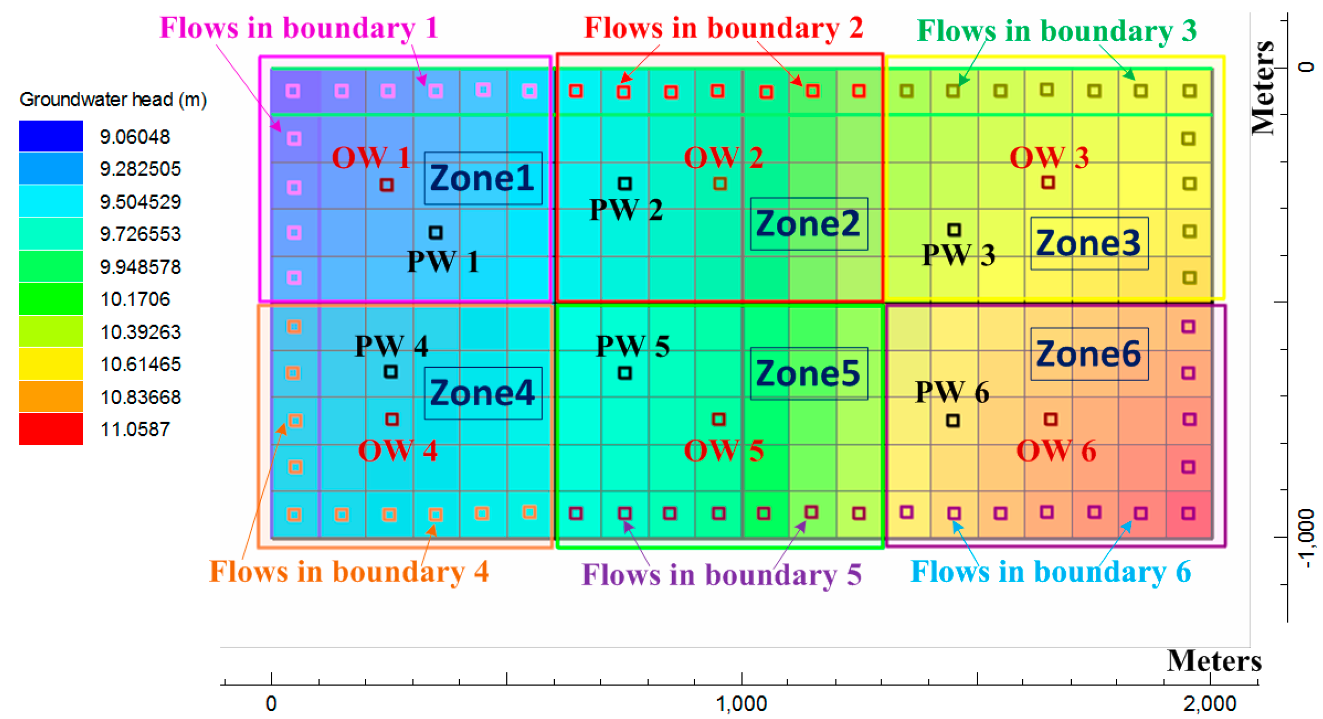To formulate the optimization model, the zonation approach [38,39] is used to partition the parameter space according to the observation well location.

Assume that the spatiotemporal pumpage pattern can be estimated beforehand, and the storage coefficients and specific yield values can be obtained from pumping tests. Then, the parameter vector estimated $\mathsf{\eta }=\left[K_{}^{\mathrm{aqu}},K_{}^{\mathrm{riv}},K_{}^{\mathrm{V}},R_{}^{\mathrm{surf}},R_{}^{\mathrm{boun}}\right]$ in the optimization model includes aquifer hydraulic conductivity $K_{}^{\mathrm{aqu}}=\left\{K_{s_f,f}^{\mathrm{aqu}}|s_f=1,\dots ,S_f;f=1,\dots ,F\right\}$, riverbed leakage conductivity $K_{}^{\mathrm{riv}}=\left\{K_{{\tau }_{\gamma },\gamma }^{\mathrm{riv}}|{\tau }_{\gamma }=1,\dots ,R_{\gamma };\gamma =1,\dots ,H\right\}$, aquitard leakance conductivity $K_{}^{\mathrm{V}}=\left\{K_{s_f,f}^{\mathrm{V}}|s_f=1,\dots ,S_f;f=1,\dots ,F\right\}$, and the source patterns of surface recharge $R_{}^{\mathrm{surf}}=\left\{R_{t_{\mathrm{s}},s_f}^{\mathrm{surf}}|s_f=1,\dots ,S_f\right\}$ and boundary recharge $R_{}^{\mathrm{boun}}=\left\{R_{t_{\mathrm{s}},{\alpha }_f,f}^{\mathrm{boun}}|{\alpha }_f=1,\dots ,B_f;f=1,\dots ,F\right\}$. The parameter vector $\mathsf{\eta }$ has L entries and $L=F\times S_f+R_f+(F-1)\times S_f+T_{\mathrm{s}}\times S_f+T_{\mathrm{s}}\times F\times B_f$ in which $K_{s_f,f}^{\mathrm{aqu}}$ is the hydraulic conductivity of aquifer f in region $s_f$ [${\mathrm{LT}}^{-1}$]; $K_{{\tau }_{\gamma },\gamma }^{\mathrm{riv}}$ is the riverbed hydraulic conductivity of river $\gamma$ in region ${\tau }_{\gamma }$ [${\mathrm{LT}}^{-1}$]; $K_{s_f,f}^{\mathrm{V}}$ is the vertical hydraulic conductivity of aquitard f in region $s_f$ [${\mathrm{T}}^{-1}$]; $R_{t_{\mathrm{s}},s_f}^{\mathrm{surf}}$ is the surface recharge of region $s_f$ for time step $t_{\mathrm{s}}$; $R_{t_{\mathrm{s}},{\alpha }_f,f}^{\mathrm{boun}}$ is the boundary recharge of aquifer f and arc ${\alpha }_f$ for time step $t_{\mathrm{s}}$ [${\mathrm{L}}^3{\mathrm{T}}^{-1}$]; and $T_{\mathrm{s}}$, $H$, $R_{\gamma }$, and $B_f$ are the total time step number, total number of rivers, total sectional number of river $\gamma$, and total boundary arcs of aquifer f, respectively.

The optimization model contains four constraints: (1) the spatiotemporal pattern of multiple recharges should subject to mass balance, (2) the simulation of groundwater head should obey governing Equation (1), (3) the upper and lower bounds of in situ hydrogeological parameters, and (4) the allocated upper and lower bounds of surface recharge. In a real case, the identification of hydrogeological parameters and recharges often form a large-scale highly nonlinear problem.

2.2. Modification of Traditional Algorithms in Nonlinear Programming for Proposing SR3 VLS Quasi-Newton Algorithm to Solve Hydrogeological Parameters

In nonlinear programming, Newton’s method attempts to find the roots of $J^{\prime }$ by constructing a sequence ${\mathsf{\eta }}^k$ from the initial guess ${\mathsf{\eta }}^0$ that converges towards some value ${\mathsf{\eta }}^{*}$ satisfying $J^{\prime }\left({\mathsf{\eta }}^{*}\right)=0$. This ${\mathsf{\eta }}^{*}$ is a stationary point of $J$ where the second-order Taylor expansion $J_{\mathrm{T}}\left({\mathsf{\eta }}^{*}\right)$ of an objective function $J$ around ${\mathsf{\eta }}^k$ is:

$$J_{\mathrm{T}}\left({\mathsf{\eta }}^{k+1}\right)=J_{\mathrm{T}}\left({\mathsf{\eta }}^k+\mathsf{\Delta }{\mathsf{\eta }}^k\right)\approx J\left({\mathsf{\eta }}^k\right)+J^{\prime }{\left({\mathsf{\eta }}^k\right)}^{\mathrm{T}}·\mathsf{\Delta }{\mathsf{\eta }}^k+\frac{1}{2}{\left(\mathsf{\Delta }{\mathsf{\eta }}^k\right)}^{\mathrm{T}}{J}^{″}\left({\mathsf{\eta }}^k\right)·\mathsf{\Delta }{\mathsf{\eta }}^k$$

(3)

Ideally, we want to pick $\mathsf{\Delta }{\mathsf{\eta }}^k$ such that ${\mathsf{\eta }}^k+\mathsf{\Delta }{\mathsf{\eta }}^k$ is a stationary point of $J$. Using this Taylor expansion as an approximation, we can at least solve for the $\mathsf{\Delta }{\mathsf{\eta }}^k$ corresponding to the root of the expansion’s derivative:

$$0=\frac{d}{d\mathsf{\Delta }{\mathsf{\eta }}^k}\left(J\left({\mathsf{\eta }}^k\right)+J^{\prime }{\left({\mathsf{\eta }}^k\right)}^{\mathrm{T}}·\mathsf{\Delta }{\mathsf{\eta }}^k+\frac{1}{2}{\left(\mathsf{\Delta }{\mathsf{\eta }}^k\right)}^{\mathrm{T}}{J}^{″}\left({\mathsf{\eta }}^k\right)·\mathsf{\Delta }{\mathsf{\eta }}^k\right)=J^{\prime }\left({\mathsf{\eta }}^k\right)+J^{″}\left({\mathsf{\eta }}^k\right)·\mathsf{\Delta }{\mathsf{\eta }}^k$$

(4)

$$\Rightarrow \mathsf{\Delta }{\mathsf{\eta }}^k=-{\left[J^{″}\left({\mathsf{\eta }}^k\right)\right]}^{-1}{J}^{\prime }\left({\mathsf{\eta }}^k\right)$$

(5)

The above-mentioned iterative scheme can be generalized to several dimensions by replacing the derivative with the gradient, $\nabla J\left({\mathsf{\eta }}^k\right)$ and the reciprocal of the second derivative with the inverse of the Hessian matrix, $H\left({\mathsf{\eta }}^k\right)J\left({\mathsf{\eta }}^k\right)$. The iterative scheme obtained on doing so is as follows:

$${\mathsf{\eta }}^{k+1}={\mathsf{\eta }}^k-{\left[H\left({\mathsf{\eta }}^k\right)J\left({\mathsf{\eta }}^k\right)\right]}^{-1}\nabla J\left({\mathsf{\eta }}^k\right),k\in \mathbb{N}$$

(6)

If all second-order partial derivatives of $J$ exist and are continuous over the function domain, then the Hessian matrix $H$ of $J$ is usually defined as follows:

$$H\left({\mathsf{\eta }}^k\right)=\left[\begin{array}{cccc}\frac{{\partial }^{2}J}{\partial {\eta }_1^2}& \frac{{\partial }^{2}J}{\partial {\eta }_1^{}\partial {\eta }_2^{}}& \cdots & \frac{{\partial }^{2}J}{\partial {\eta }_1^{}\partial {\eta }_L^{}}\\ \frac{{\partial }^{2}J}{\partial {\eta }_2^{}\partial {\eta }_1^{}}& \frac{{\partial }^{2}J}{\partial {\eta }_2^2}& \cdots & \frac{{\partial }^{2}J}{\partial {\eta }_2^{}\partial {\eta }_L^{}}\\ ⋮& ⋮& \ddots & ⋮\\ \frac{{\partial }^{2}J}{\partial {\eta }_L^{}\partial {\eta }_1^{}}& \frac{{\partial }^{2}J}{\partial {\eta }_L^{}\partial {\eta }_2^{}}& \cdots & \frac{{\partial }^{2}J}{\partial {\eta }_L^2}\end{array}\right]$$

(7)

At a local minimum, the Hessian is positive semi-definite. The geometric interpretation of the Gauss–Newton method is that at each iteration, $J_{\mathrm{T}}\left({\mathsf{\eta }}^k\right)$ is approximated by a quadratic function around ${\mathsf{\eta }}^k$, and a small scalar step size $\alpha \in \left(0,1\right)$ was taken to the minimum (or maximum) of that function, as expressed in Equation (8a). The Jacobian quasi-Newton method uses the Jacobian matrix $J_{\mathrm{D}}$ to approximate the Hessian matrix $H\approx 2J_{\mathrm{D}}^{\mathrm{T}}{J}_{\mathrm{D}}^{}$ iteratively, as expressed in Equation (8b). The Levenberg–Marquardt algorithm adds an identity matrix $I$ to the Hessian $H\approx J_{\mathrm{D}}^{\mathrm{T}}{J}_{\mathrm{D}}^{}+\lambda I$, with the scale adjusted iteratively as needed, in which the increment vector is rotated towards the direction of steepest descent, as expressed in Equation (8c). Considering a disadvantage arises for large damping factor values $\lambda$, Fletcher (1971) proposed each gradient component can be scaled by curvature, so that there is larger movement along directions where the gradient is smaller [17], which avoids slow convergence in the direction of a small gradient. Therefore, the identity matrix was replaced with the diagonal matrix comprising diagonal elements of $J_{\mathrm{D}}^{\mathrm{T}}{J}_{\mathrm{D}}^{}$, which is used to solve linear ill-posed problems, as expressed in Equation (8d). The BFGS quasi-Newton algorithm is used for solving unconstrained nonlinear optimization problems by setting the search direction $d^k=-H^{-1}\left({\mathsf{\eta }}^k\right)\nabla J\left({\mathsf{\eta }}^k\right)\approx -A^{-1}\left({\mathsf{\eta }}^k\right)\nabla J\left({\mathsf{\eta }}^k\right)$ for the analog solution of the Newton equation, where $A\left({\mathsf{\eta }}^k\right)$ approximates the Hessian matrix, as expressed in Equation (8e).

$${\mathsf{\eta }}^{k+1}={\mathsf{\eta }}^k-{\alpha }^k{\left[H\left({\mathsf{\eta }}^k\right)J\left({\mathsf{\eta }}^k\right)\right]}^{-1}\nabla J\left({\mathsf{\eta }}^k\right),k\in \mathbb{N}$$

(8a)

$${\mathsf{\eta }}^{k+1}={\mathsf{\eta }}^k-{\alpha }^k{\left[2J_{\mathrm{D}}^{\mathrm{T}}{J}_{\mathrm{D}}^{}\right]}^{-1}{J}_{\mathrm{D}}^{\mathrm{T}}r\left({\mathsf{\eta }}^k\right),k\in \mathbb{N}$$

(8b)

$${\mathsf{\eta }}^{k+1}={\mathsf{\eta }}^k-{\left[J_{\mathrm{D}}^{\mathrm{T}}{J}_{\mathrm{D}}^{}+\lambda I\right]}^{-1}{J}_{\mathrm{D}}^{\mathrm{T}}r\left({\mathsf{\eta }}^k\right),k\in \mathbb{N}$$

(8c)

$${\mathsf{\eta }}^{k+1}={\mathsf{\eta }}^k-{\left[J_{\mathrm{D}}^{\mathrm{T}}{J}_{\mathrm{D}}^{}+\lambda \mathrm{diag}(J_{\mathrm{D}}^{\mathrm{T}}{J}_{\mathrm{D}}^{})\right]}^{-1}{J}_{\mathrm{D}}^{\mathrm{T}}r({\mathsf{\eta }}^k),k\in \mathbb{N}$$

(8d)

$${\mathsf{\eta }}^k={\mathsf{\eta }}^{k-1}+A^{-1}\left({\mathsf{\eta }}^k\right)·\left[\nabla J\left({\mathsf{\eta }}^k\right)-\nabla J\left({\mathsf{\eta }}^{k-1}\right)\right],k\in \mathbb{N}$$

(8e)

$${\mathsf{\eta }}^{k+1}={\mathsf{\eta }}^k-{\mathsf{\alpha }}^k\circ \left\{{\left[{\left({\Psi }_{\mathrm{D}}^{\mathrm{T}}\right)}^k{\Psi }_{\mathrm{D}}^k+{\mathsf{\theta }}^k\circ {\left({\Gamma }_{\mathrm{D}}^{\mathrm{T}}\right)}^k{\Gamma }_{\mathrm{D}}^k+{\mathsf{\omega }}^k\circ {\left({\Psi }_{\mathrm{D}}^{\mathrm{T}}\right)}^k{\Gamma }_{\mathrm{D}}^k\right]}^{-1}·{\left(J_{\mathrm{D}}^{\mathrm{T}}\right)}^k·r\left({\mathsf{\eta }}^k\right)\right\},k\in \mathbb{N}$$

(8f)

To accelerate convergence, jump over local minima, and achieve a well-posed problem, this study uses a vectorized limited switchable step size ${\mathsf{\alpha }}^k=\left[{\alpha }_l^k|l=1~L\right]\in \left(-{\epsilon }_l^k,{\epsilon }_l^k\right)$ in the inverse problem of transmissive groundwater whose parameters include both hydrogeology and source simultaneously. Therefore, we achieve $\left|r_m\frac{{\partial }^2{r}_m}{\partial {\eta }_i\partial {\eta }_j}\right|\approx \left|\frac{\partial r_m}{\partial {\eta }_i}\frac{\partial r_m}{\partial {\eta }_j}+\mathrm{SVD}\left({\vartheta }_m^k-{\vartheta }_m^{k-1},{\eta }_l^k-{\eta }_l^{k-1}\right)\right|$, detect the minima area, approach global optimum, and solve nonlinear ill-posed problems, this study modifies LMA and imports a third rank structure from BFGS for solving constrained nonlinear parameter identification problems, which uses a low-rank factor loading score ${\Psi }_{\mathrm{D}}^{}$ and a high-rank loading score ${\Gamma }_{\mathrm{D}}^{}$ analyzed from the simulated storage difference ${\vartheta }_m^k-{\vartheta }_m^{k-1}$ to approximate the Hessian and calculate the correction matrix, as expressed in Equation (8f).

In Equation (8b–d), $J_{\mathrm{D}}^{\mathrm{T}}\left({\mathsf{\eta }}^k\right)$ is the Jacobian matrix of ${\vartheta }_m^{\mathrm{sim}}$ defined in Equation (9a). In Equation (8e), set $y^{k-1}=\nabla J\left({\mathsf{\eta }}^k\right)-\nabla J\left({\mathsf{\eta }}^{k-1}\right)$ and $s^{k-1}={\mathsf{\eta }}^k-{\mathsf{\eta }}^{k-1}$, the approximate Hessian matrix $A\left({\mathsf{\eta }}^k\right)$ in the BFGS algorithm is updated by the addition of two matrices as expressed in Equation (9b), subjected to symmetry and positive definiteness of $A\left({\mathsf{\eta }}^k\right)$. Both ${\chi }^k{\mathsf{\mu }}^{k-1}{\left({\mathsf{\mu }}^{k-1}\right)}^{\mathrm{T}}$ and ${\gamma }^k{\mathsf{\nu }}^{k-1}{\left({\mathsf{\nu }}^{k-1}\right)}^{\mathrm{T}}$ are symmetric rank-one matrices, and their sum is a rank two updated matrix. Imposing the secant condition [40] $A\left({\mathsf{\eta }}^k\right)·s^{k-1}=y^{k-1}$ and choosing ${\mathsf{\mu }}^{k-1}=y^{k-1}$ and ${\mathsf{\nu }}^{k-1}=A\left({\mathsf{\eta }}^{k-1}\right)·s^{k-1}$, the secant BFGS scale factors ${\chi }^k$ and ${\gamma }^k$ are expressed in Equation (9c).

$$J_{\mathrm{D}}^{\mathrm{T}}\left({\mathsf{\eta }}^k\right)={\left[\begin{array}{cccccc}\frac{\partial {\vartheta }_1^{\mathrm{sim}}}{\partial {\eta }_1}& \frac{\partial {\vartheta }_2^{\mathrm{sim}}}{\partial {\eta }_1}& \cdots & \frac{\partial {\vartheta }_m^{\mathrm{sim}}}{\partial {\eta }_1}& \cdots & \frac{\partial {\vartheta }_M^{\mathrm{sim}}}{\partial {\eta }_1}\\ ⋮& ⋮& & ⋮& & ⋮\\ \frac{\partial {\vartheta }_1^{\mathrm{sim}}}{\partial {\eta }_L}& \frac{\partial {\vartheta }_2^{\mathrm{sim}}}{\partial {\eta }_L}& \cdots & \frac{\partial {\vartheta }_m^{\mathrm{sim}}}{\partial {\eta }_L}& \cdots & \frac{\partial {\vartheta }_M^{\mathrm{sim}}}{\partial {\eta }_L}\end{array}\right]}_{L\times M}$$

(9a)

$$A\left({\mathsf{\eta }}^k\right)=A\left({\mathsf{\eta }}^{k-1}\right)+{\chi }^k{\mathsf{\mu }}^{k-1}{\left({\mathsf{\mu }}^{k-1}\right)}^{\mathrm{T}}+{\gamma }^k{\mathsf{\nu }}^{k-1}{\left({\mathsf{\nu }}^{k-1}\right)}^{\mathrm{T}}$$

(9b)

$${\chi }^k=\frac{1}{{\left(y^{k-1}\right)}^{\mathrm{T}}{s}^{k-1}},{\gamma }^k=-\frac{1}{{\left(s^{k-1}\right)}^{\mathrm{T}}·A\left({\mathsf{\eta }}^{k-1}\right)·s^{k-1}}$$

(9c)

In the proposing SR3 VLS quasi-Newton algorithm in Equation (8f), ${\left({\Psi }_{\mathrm{D}}^{\mathrm{T}}\right)}^k{\Psi }_{\mathrm{D}}^k$, ${\mathsf{\theta }}^k\circ {\left({\Gamma }_{\mathrm{D}}^{\mathrm{T}}\right)}^k{\Gamma }_{\mathrm{D}}^k$ and ${\mathsf{\omega }}^k\circ {\left({\Psi }_{\mathrm{D}}^{\mathrm{T}}\right)}^k{\Gamma }_{\mathrm{D}}^k$ are symmetric rank-one matrices; however, their sum is a rank three matrix. The row vectors of the low-rank and high-rank loading score matrix, namely ${\left({\Psi }_{\mathrm{D}}^{\mathrm{T}}\right)}^k$ and ${\left({\Gamma }_{\mathrm{D}}^{\mathrm{T}}\right)}^k$, are permutated from ${\left({\Psi }_{\mathrm{D},l}^{\mathrm{T}}\right)}^k$ and ${\left({\Gamma }_{\mathrm{D},l}^{\mathrm{T}}\right)}^k$, as expressed in Equation (10a–c) and in Equation (10d–f), respectively, in which the low-rank component j is 1, and the high-rank component j is from 2 to S_f. This study uses the factor score ${\left(\widetilde{C_{·,·,f}^{}}\right)}^k$ and the factor loading ${\left(F_{·,·,f}^{\mathrm{T}}\right)}^k$ calculated from the simulated storage difference ${\vartheta }_m^k-{\vartheta }_m^{k-1}$ through SVD between iteration k and k − 1 to compute the elements of ${\left({\Psi }_{\mathrm{D},l}^{\mathrm{T}}\right)}^k$ and ${\left({\Gamma }_{\mathrm{D},l}^{\mathrm{T}}\right)}^k$, as expressed in Equations (13)–(16), thereby eliminating the need for additional model runs to approximate the Hessian. $D_{·,f}^k$ is the diagonalized standard deviation matrix of ${\vartheta }_m^k-{\vartheta }_m^{k-1}$, where $m=1,2,\dots ,M$, and $M=T_{\mathrm{s}}\times S_f\times F$. Before SVD, the simulated storage difference ${\vartheta }_m^k-{\vartheta }_m^{k-1}$ will first be normalized by the average $a^k$ and standard deviation ${\epsilon }_l^k$ for each zonal $s_f$ and each aquifer f across multiple simulated time steps $t_{\mathrm{s}}$, such that the average of the simulated storage difference of each zone equals to 0 and the variance equals to 1. Hence, the vectorized step size ${\mathsf{\alpha }}^k$ is a switchable and limited set between $-{\epsilon }_l^k$ and ${\epsilon }_l^k$, namely ${\mathsf{\alpha }}^k=\left[{\alpha }_l^k|l=1~L\right]\in \left(-{\epsilon }_l^k,{\epsilon }_l^k\right)$.

$${\left({\Psi }_{\mathrm{D},l}^{\mathrm{T}}\right)}^k=\left[Y_{1,1,l}^{},Y_{1,2,l}^{},\cdots Y_{1,t_{\mathrm{s}},l}^{},\cdots Y_{1,T_{\mathrm{s}},l}^{},\cdots Y_{s_f,1,l}^{},\cdots Y_{s_f,t_{\mathrm{s}},l}^{},\cdots Y_{s_f,T_{\mathrm{s}},l}^{},\cdots Y_{S_f,1,l}^{},\cdots Y_{S_f,t_{\mathrm{s}},l}^{},\cdots Y_{S_f,T_{\mathrm{s}},l}^{}\right]$$

(10a)

$$Y_{s_f,t_{\mathrm{s}},l}^{}={\displaystyle \sum _{t=1}^{t_{\mathrm{s}}}{Y}_{s_f,t_{},l}^{}}$$

(10b)

$${\left({\Psi }_{·,·,l}^{\mathrm{T}}\right)}^k=\frac{1}{{\eta }_l^k-{\eta }_l^{k-1}}\left[{\left(\widetilde{C_{1,·,f}^{}}\right)}^k{\left(F_{1,·,f}^{\mathrm{T}}\right)}^k{D}_{·,f}^k-{\left[\begin{array}{c}1\\ ⋮\\ 1\end{array}\right]}_{T_{\mathrm{s}}\times 1}·{\left(\widetilde{C_{1,1,f}^{}}\right)}^k{\left(F_{1,·,f}^{\mathrm{T}}\right)}^k{D}_{·,f}^k\right]$$

(10c)

$${\left({\Gamma }_{\mathrm{D},l}^{\mathrm{T}}\right)}^k=\left[G_{1,1,l}^{},G_{1,2,l}^{},\cdots G_{1,t_{\mathrm{s}},l}^{},\cdots G_{1,T_{\mathrm{s}},l}^{},\cdots G_{s_f,1,l}^{},\cdots G_{s_f,t_{\mathrm{s}},l}^{},\cdots G_{s_f,T_{\mathrm{s}},l}^{},\cdots G_{S_f,1,l}^{},\cdots G_{S_f,t_{\mathrm{s}},l}^{},\cdots G_{S_f,T_{\mathrm{s}},l}^{}\right]$$

(10d)

$$G_{s_f,t_{\mathrm{s}},l}^{}={\displaystyle \sum _{t=1}^{t_{\mathrm{s}}}{G}_{s_f,t_{},l}^{}}$$

(10e)

$${\left({\Gamma }_{·,·,l}^{\mathrm{T}}\right)}^k=\frac{1}{{\eta }_l^k-{\eta }_l^{k-1}}\left[{\left(\widetilde{C_{j,·,f}^{}}\right)}^k{\left(F_{j,·,f}^{\mathrm{T}}\right)}^k{D}_{·,f}^k-{\left[\begin{array}{c}1\\ ⋮\\ 1\end{array}\right]}_{T_{\mathrm{s}}\times 1}·{\left(\widetilde{C_{j,1,f}^{}}\right)}^k{\left(F_{j,·,f}^{\mathrm{T}}\right)}^k{D}_{·,f}^k\right]$$

(10f)

According to this design, this study uses the orthogonal component of loading scores ${\left({\Gamma }_{\mathrm{D}}^{\mathrm{T}}\right)}^k$ and ${\left({\Psi }_{\mathrm{D}}^{\mathrm{T}}\right)}^k$ to correct the direction to better approximate the Hessian. That is, the modified algorithm uses the vector-expanded matrix ${\mathsf{\theta }}^k$ and ${\mathsf{\omega }}^k$ to scale each high-rank component of the loading scores according to the orthogonal properties eigenvalue ${\tau }_j^k$ to approximate the Hessian and explore different local minima positions, so there is larger movement along the directions for each parameter where the gradient is smaller. Accordingly, this study designs the symmetry rank three loading scores ${\left({\Psi }_{\mathrm{D}}^{\mathrm{T}}\right)}^k{\Psi }_{\mathrm{D}}^k$, ${\mathsf{\theta }}^k\circ {\left({\Gamma }_{\mathrm{D}}^{\mathrm{T}}\right)}^k{\Gamma }_{\mathrm{D}}^k$, and ${\mathsf{\omega }}^k\circ {\left({\Psi }_{\mathrm{D}}^{\mathrm{T}}\right)}^k{\Gamma }_{\mathrm{D}}^k$ to solve nonlinear ill-posed problems, thus, properly handling the approximated Hessian elements by scale and correction at all iterations. The calculation of the scale matrix ${\mathsf{\theta }}^k$ and ${\mathsf{\omega }}^k$ are formulated as follows:

$${\mathsf{\theta }}^k={\left[\frac{{\tau }_1^k}{{\tau }_j^k}|\begin{array}{l}\\ j=1~S_f\end{array}\right]}_{L\times 1}{\left[1,1,\cdots ,1\right]}_{1\times L}$$

(11a)

$${\mathsf{\omega }}^k=2{\left[\sqrt{\frac{{\tau }_1^k}{{\tau }_j^k}}|\begin{array}{l}\\ j=1~S_f\end{array}\right]}_{L\times 1}{\left[1,1,\cdots ,1\right]}_{1\times L}$$

(11b)

In large-scale groundwater modeling with a large number of parameters and numerical grids, the transient simulation time increases substantially [41]. To imitate the real complex alluvial groundwater hydrogeology in practice, meticulously detailed parameterization of aquifer’s/aquitard’s shape is unavoidable. Hence, computing and storing the full Hessian matrix directly may be infeasible, unavailable, and too expensive to compute at all iterations in hydrogeological parameter identification. Furthermore, the convergence of the Jacobian quasi-Newton is not guaranteed. The approximation $\left|r_m\frac{{\partial }^2{r}_m}{\partial {\eta }_i\partial {\eta }_j}\right|\ll \left|\frac{\partial r_m}{\partial {\eta }_i}\frac{\partial r_m}{\partial {\eta }_j}\right|$ required to ignore the second-order derivative terms may be valid in two conditions [17], for which convergence is to be expected: the function values $r_m$ are small in magnitude, at least around the minimum; and the functions are only slightly nonlinear, so that $\frac{{\partial }^2{r}_m}{\partial {\eta }_i\partial {\eta }_j}$ is relatively small in magnitude. Moreover, when the (non-negative) Marquardt damping factor $\lambda$ (scalar) optimized by a line search changes, the shift vector must be recalculated. Furthermore, in cases with multiple minima, the algorithm converges to the global minimum only if the initial guess is close to the final solution [20]. However, for well-behaved functions and reasonable starting parameters, the LMA tends to be slightly slower than the Jacobian quasi-Newton. Besides, letting $A\left({\mathsf{\eta }}^{k+1}\right)$ be positive definite in the BFGS updates should satisfy the curvature condition ${\left(s^{k-1}\right)}^{\mathrm{T}}{y}^{k-1}>0$ and $A\left({\mathsf{\eta }}^k\right)$ be positive definite. A key reason leading to the above challenges is the scalar nature of the step size ${\alpha }^k$ in the Jacobian quasi-Newton, the Marquardt damping factor $\lambda$ in LMA, and the secant scale factors ${\beta }^k$ and ${\gamma }^k$ in BFGS. Hence, this study uses the designed preserved approximate Hessians with positive definite and numerically stable selections from the various combinations of low–high rank loading scores along with the vectorized limited switchable step sizes to detect the area of the global minimum and approach the global optimum in a multi-minima problem.

2.3. Modification from Traditional Scalar Line Search to Vectorized Multi-Order Derivative Exact Double False Position Bracketing Using SVD-Related Rank and Depth

The traditional double false position provides the exact solution for a root-finding problem, which determines a scalar ${\alpha }^k\in \left[{\alpha }_{*}^{k,\kappa }|\kappa =1~\mathrm{\Sigma }\right],$ such that $J^{\prime }({\alpha }_{*}^{k,\kappa })=0$, while a nonlinear objective function $J^{\prime }$ can be successively improved by iteration $\kappa$. If $J^{\prime }$ is a continuous function and there exist two points ${\alpha }_{\mathrm{LB}}^{k,\kappa }$ and ${\alpha }_{\mathrm{UB}}^{k,\kappa }$ such that $J^{\prime }\left({\alpha }_{\mathrm{LB}}^{k,\kappa }\right)$ and $J^{\prime }\left({\alpha }_{\mathrm{UB}}^{k,\kappa }\right)$ are of opposite signs, then, by the intermediate value theorem, the function $J^{\prime }$ has a root ${\alpha }_{*}^{k,\kappa }$ in the interval $\left[{\alpha }_{\mathrm{LB}}^{k,\kappa },{\alpha }_{\mathrm{UB}}^{k,\kappa }\right]$. The simplest two-point bracketing is the bisection method, which estimates the solution as the bracketing interval midpoint as expressed in Equation (12a). If the functional value of the new calculated estimate ${\alpha }_{\mathrm{MP}}^{k,\kappa }$ has the same sign as $J^{\prime }\left({\alpha }_{\mathrm{UB}}^{k,\kappa }\right)$, the new bracketing interval becomes $\left[{\alpha }_{\mathrm{LB}}^{k,\kappa +1},{\alpha }_{\mathrm{UB}}^{k,\kappa +1}\right]=\left[{\alpha }_{\mathrm{LB}}^{k,\kappa },{\alpha }_{\mathrm{MP}}^{k,\kappa }\right]$. The fact that false position method always converges, and has advantages that minimize slowdowns, recommends it when speed is needed [22], in which the solved ${\alpha }_{\mathrm{MP}}^{k,\kappa }$ is expressed in Equation (12b). The Illinois algorithm dampens one of the endpoint values by a factor of 1/2 to force the next ${\alpha }_{\mathrm{MP}}^{k,\kappa }$ to occur on that side of $J^{\prime }\left({\alpha }_{\mathrm{LB}}^{k,\kappa }\right)$ guaranteeing superlinear convergence, as shown in Equation (12c). The Anderson−Bjork algorithm multiplies $J^{\prime }\left({\alpha }_{\mathrm{LB}}^{k,\kappa }\right)$ by m in Equation (12c), as expressed in Equation (12d).

For the vectorized step size root finding problem, which is more difficult and complicated, the double false position can be used and written algebraically in the form: determine ${\mathsf{\alpha }}^k\in \left[{\mathsf{\alpha }}_{*}^{k,\kappa }|\kappa =1~\mathrm{\Sigma }\right]$ such that $J^{\prime }\left(•,{\mathsf{\alpha }}_{*}^{k,\kappa }\right)=0$, if the known conditions are $J^{\prime }\left(•,{\mathsf{\alpha }}_{LB}^{k,\kappa }\right)=b_1,J^{\prime }\left(•,{\mathsf{\alpha }}_{UB}^{k,\kappa }\right)=b_2$ at the $\kappa$-th iteration in the exact optimization procedure of the vectorized step size. If $J^{\prime }\left(•,{\mathsf{\alpha }}_{*}^{k,\kappa }\right)$ is a nonlinear continuous function and there exist two vectors ${\mathsf{\alpha }}_{LB}^{k,\kappa }$ and ${\mathsf{\alpha }}_{UB}^{k,\kappa }$ such that each corresponding element of vectors $J^{\prime }\left(•,{\mathsf{\alpha }}_{LB}^{k,\kappa }\right)$ and $J^{\prime }\left(•,{\mathsf{\alpha }}_{UB}^{k,\kappa }\right)$ are of opposite signs, then by the intermediate value theorem, the function $J^{\prime }\left(•,{\mathsf{\alpha }}_{*}^{k,\kappa }\right)$ has a root ${\mathsf{\alpha }}_{*}^{k,\kappa }$ in the interval $\left[{\mathsf{\alpha }}_{LB}^{k,\kappa },{\mathsf{\alpha }}_{UB}^{k,\kappa }\right]$. In a conventional iterative nonlinear programming for parameter identification, the information $J\left({\mathsf{\eta }}^k\right)$ in Equation (6) is not used for exact approximation. Hence, this study modifies the double false position method for estimating new parameter vector guesses ${\mathsf{\alpha }}_{MP}^{k,\kappa }=\left[{\alpha }_{\mathrm{MP},l}^{k,\kappa }|l=1~L\right]$ through a series of non-derivative, first-order derivative, and SVD depth component-based halving vectors of the objective function simultaneously in vector form, as shown in Equation (12e).

$${\alpha }_{\mathrm{MP}}^{k,\kappa }=\frac{{\alpha }_{\mathrm{LB}}^{k,\kappa }+{\alpha }_{\mathrm{UB}}^{k,\kappa }}{2}$$

(12a)

$${\alpha }_{\mathrm{MP}}^{k,\kappa }=\frac{{\alpha }_{\mathrm{LB}}^{k,\kappa }{J}^{\prime }\left({\alpha }_{\mathrm{UB}}^{k,\kappa }\right)-{\alpha }_{\mathrm{UB}}^{k,\kappa }{J}^{\prime }\left({\alpha }_{\mathrm{LB}}^{k,\kappa }\right)}{J^{\prime }\left({\alpha }_{\mathrm{UB}}^{k,\kappa }\right)-J^{\prime }\left({\alpha }_{\mathrm{LB}}^{k,\kappa }\right)}$$

(12b)

$${\alpha }_{\mathrm{MP}}^{k,\kappa }=\frac{{\alpha }_{\mathrm{LB}}^{k,\kappa }{J}^{\prime }\left({\alpha }_{\mathrm{UB}}^{k,\kappa }\right)-\frac{1}{2}{\alpha }_{\mathrm{UB}}^{k,\kappa }{J}^{\prime }\left({\alpha }_{\mathrm{LB}}^{k,\kappa }\right)}{J^{\prime }\left({\alpha }_{\mathrm{UB}}^{k,\kappa }\right)-\frac{1}{2}{J}^{\prime }\left({\alpha }_{\mathrm{LB}}^{k,\kappa }\right)}$$

(12c)

$${\alpha }_{\mathrm{MP}}^{k,\kappa }=\frac{{\alpha }_{\mathrm{LB}}^{k,\kappa }{J}^{\prime }\left({\alpha }_{\mathrm{UB}}^{k,\kappa }\right)-m·{\alpha }_{\mathrm{UB}}^{k,\kappa }{J}^{\prime }\left({\alpha }_{\mathrm{LB}}^{k,\kappa }\right)}{J^{\prime }\left({\alpha }_{\mathrm{UB}}^{k,\kappa }\right)-m·J^{\prime }\left({\alpha }_{\mathrm{LB}}^{k,\kappa }\right)},s.t.\{\begin{array}{c}m=1-\frac{J^{\prime }\left({\alpha }_{\mathrm{MP}}^{k,\kappa }\right)}{J^{\prime }\left({\alpha }_{\mathrm{UB}}^{k,\kappa }\right)},\begin{array}{cc}& if\begin{array}{cc}& m>0\end{array}\end{array}\\ m=1/2,\begin{array}{cc}& else\end{array}\end{array}$$

(12d)

$${\alpha }_{\mathrm{MP},l}^{k,\kappa }=\frac{{\mathsf{\zeta }}_l·\left[{\mathsf{\alpha }}_{LB}^{k,\kappa }\circ \nabla J\left(•,{\mathsf{\alpha }}_{UB}^{k,\kappa }\right)-m_p\circ {\mathsf{\alpha }}_{UB}^{k,\kappa }\circ \nabla J\left(•,{\mathsf{\alpha }}_{LB}^{k,\kappa }\right)\right]}{{\mathsf{\zeta }}_l·\left[\nabla J\left(•,{\mathsf{\alpha }}_{UB}^{k,\kappa }\right)-m_p\circ \nabla J\left(•,{\mathsf{\alpha }}_{LB}^{k,\kappa }\right)\right]}$$

(12e)

$$m_1=\frac{J\left({\mathsf{\eta }}^k,{\mathsf{\alpha }}_{LB}^{k,\kappa }\right)}{J\left({\mathsf{\eta }}^k,{\mathsf{\alpha }}_{UB}^{k,\kappa }\right)}·{\left[\begin{array}{c}1\\ ⋮\\ 1\end{array}\right]}_{L\times 1},m_2={\left[\begin{array}{c}1-\frac{{\mathsf{\zeta }}_1·\nabla J\left(•,{\mathsf{\alpha }}_{MP}^{k,\kappa }\right)}{{\mathsf{\zeta }}_1·\nabla J\left(•,{\mathsf{\alpha }}_{UB}^{k,\kappa }\right)}\\ ⋮\\ 1-\frac{{\mathsf{\zeta }}_l·\nabla J\left(•,{\mathsf{\alpha }}_{MP}^{k,\kappa }\right)}{{\mathsf{\zeta }}_l·\nabla J\left(•,{\mathsf{\alpha }}_{UB}^{k,\kappa }\right)}\\ ⋮\\ 1-\frac{{\mathsf{\zeta }}_L·\nabla J\left(•,{\mathsf{\alpha }}_{MP}^{k,\kappa }\right)}{{\mathsf{\zeta }}_L·\nabla J\left(•,{\mathsf{\alpha }}_{UB}^{k,\kappa }\right)}\end{array}\right]}_{L\times 1},\begin{array}{c}\begin{array}{l}\\ \\ m_3={\left[\begin{array}{c}1/2\\ ⋮\\ 1/2\end{array}\right]}_{L\times 1},m_4={\left[\begin{array}{c}1\\ ⋮\\ 1\end{array}\right]}_{L\times 1},m_5={\left[\begin{array}{c}{\varpi }_1\\ ⋮\\ {\varpi }_l\\ ⋮\\ {\varpi }_L\end{array}\right]}_{L\times 1}\end{array}\\ ,{\varpi }_l\in \left[\raisebox{1ex}{$1$}\!\left/ \!\raisebox{-1ex}{$j_l·d_l$}\right.,\raisebox{1ex}{$1$}\!\left/ \!\raisebox{-1ex}{$d_l$}\right.,\raisebox{1ex}{$1$}\!\left/ \!\raisebox{-1ex}{$j_l$}\right.,\raisebox{1ex}{$d_l$}\!\left/ \!\raisebox{-1ex}{$j_l$}\right.,1/2,1\right]\end{array}$$

(12f)

where ${\mathsf{\zeta }}_l$ is the l^th unit vector; $m_1$ is the halving vector of the proposing 0 order derivative’s double false position method; $m_2$, $m_3$, and $m_4$ are the halving vectors of the vectorized Anderson−Björk algorithm, vectorized Illinois algorithm, and vectorized conventional false position method, respectively [22]; and $m_5$ is the halving vector of the proposing SVD depth rank component-based double false position method, which uses the j^th component in d^th depth as the high-rank loading score ${\Gamma }_{\mathrm{D}}^k$ for the Hessian correction.

This study uses symmetry rank three loading score quasi-Newton associated with vectorized step size for solving massive parameters in transmissive groundwater. This study specializes the step size for each parameter with a switchable limited scheme; thus, this approach helps reduce the difference between different kinds of parameters (transmissivity and source/sink) and improves the convergence rate and searching direction by modifying the parameter step size. To achieve small error in the large parameters ${\mathsf{\eta }}^{k+1}$ and the desired rapid convergence in the objective function $J\left({\mathsf{\eta }}^{k+1}\right)$, an exact line search approach, which computes the vectorized limited switchable step size that optimizes how far vector of parameters ${\mathsf{\eta }}^k$ should move along the calculated direction, is proposing. This study proposes a systematic strengthening approach of vectorized multi-order derivative exact double false position bracketing using SVD-related rank and depth, which guarantee convergence for solving the vectorized step size corresponding to different kinds of hydrogeological parameters and recharges. The detailed procedure is listed in Step 4 of Section 2.4.

2.4. Procedures of the Methodology

Step 1: Set the iteration counter $k=0$ of identified parameters ${\mathsf{\eta }}^k=\left[K_k^{\mathrm{aqu}},K_k^{\mathrm{riv}},K_k^{\mathrm{V}},R_k^{\mathrm{surf}},R_k^{\mathrm{boun}}\right]$, and make an initial guess ${\mathsf{\eta }}^0$ for the minimum.

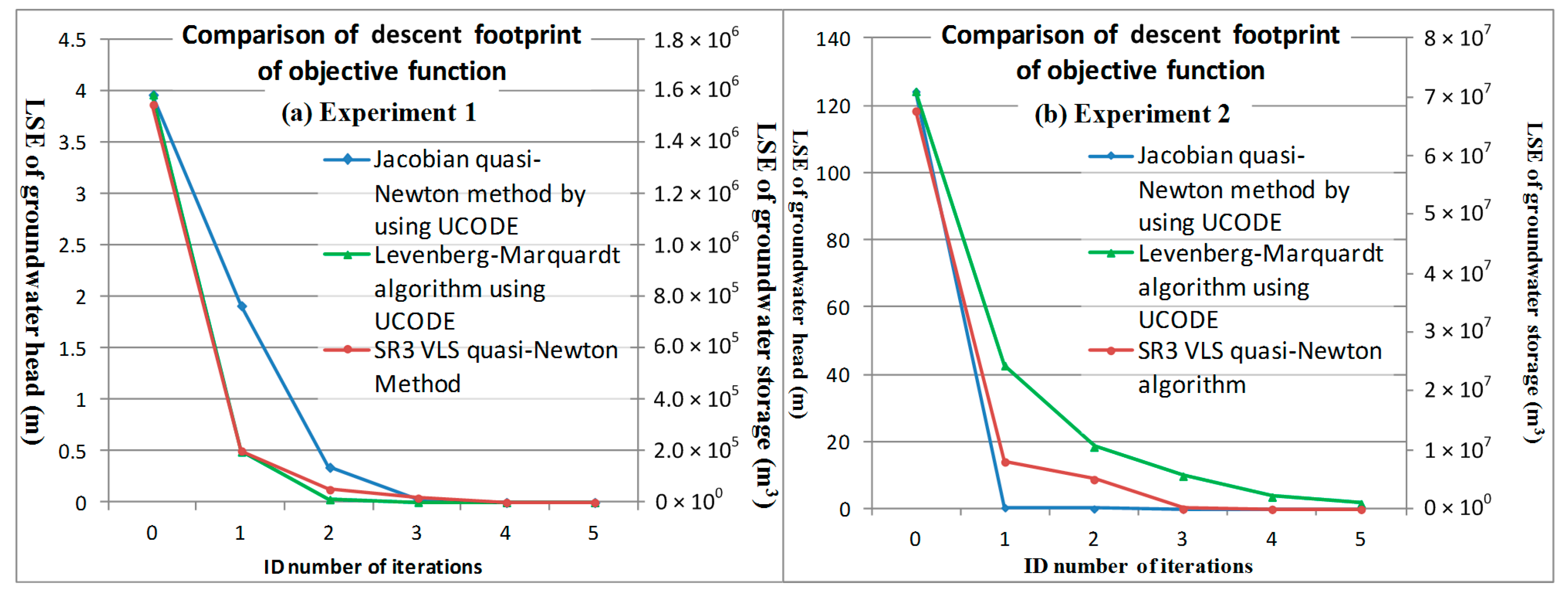
Step 1-1: In hypothetical experiment 1, the initial guess of ${\mathsf{\eta }}^k$ is set as a relatively large value.

Step 1-2: In hypothetical experiment 2, the initial guesses of $R_k^{\mathrm{surf}}$ and $R_k^{\mathrm{boun}}$ are set as mean values of the calculated lumped recharge, and those of $K_k^{\mathrm{aqu}},K_k^{\mathrm{riv}}$, and $K_k^{\mathrm{V}}$ are set as medium guess values.

Step 1-3: In practical application, the spatiotemporal recharge pattern is estimated by multiplying the temporal pattern calculated by using the lumped storage hydrograph fluctuation and the previously estimated pumpage according to Hsu et al. [16], with the initial guess of the spatial pattern estimated according to the factor loadings calculated from the computed distributed inflow hydrographs ($\mathsf{\Delta }$storage + pumpage). The initial estimate of the hydrogeological parameters is assigned according to the in situ pumping tests.

Step 2: Compute the second-order derivative descent direction $d^k={\left[{\left({\Psi }_{\mathrm{D}}^{\mathrm{T}}\right)}^k{\Psi }_{\mathrm{D}}^k+{\mathsf{\theta }}^k\circ {\left({\Gamma }_{\mathrm{D}}^{\mathrm{T}}\right)}^k{\Gamma }_{\mathrm{D}}^k+{\mathsf{\omega }}^k\circ {\left({\Psi }_{\mathrm{D}}^{\mathrm{T}}\right)}^k{\Gamma }_{\mathrm{D}}^k\right]}^{-1}·{\left(J_{\mathrm{D}}^{\mathrm{T}}\right)}^k·r\left({\mathsf{\eta }}^k\right)$ through the symmetry rank three storage-based loading scores.

Step 2-1: Simulate the spatiotemporal groundwater head pattern by using the MODFLOW from pumpage, recharge and parameters, boundary conditions, and initial conditions. The modular MODFLOW-2005, which is a computer code that solves the groundwater flow equation, was used to simulate the finite-difference flow through aquifers [42].

Step 2-2: Compute lumped and distributed groundwater storage hydrographs, based on the in situ storage coefficient and specific yield (S_y) estimated from pumping tests, drilled hydrogeological structure, and observed/simulated groundwater head hydrographs.

Step 2-3: Use various multi-rank loading score combinations calculated from the simulated storage difference ${\vartheta }_m^k-{\vartheta }_m^{k-1}$ using SVD between iteration k and k − 1 to approximate Hessians, and then use selected positive definite and numerically stable approximations with calculated $d^k$ to search for the global minimum.

Step 3: Choose ${\mathsf{\alpha }}^k$ to minimize $f\left({\mathsf{\eta }}^k+{\mathsf{\alpha }}^k\circ d^k\right)$ over ${\mathsf{\alpha }}^k=\left[{\alpha }_l^k|l=1~L\right]\in \left[{\alpha }_l^{k,\kappa }|\kappa =1~\mathrm{\Sigma }\right]\in \left(-{\epsilon }_l^k,{\epsilon }_l^k|l=1~L\right)=\left[-{\mathsf{\epsilon }}_{}^k,{\mathsf{\epsilon }}_{}^k\right]$.

Step 3-1: Set the root-finding iteration counter $\kappa =0$ and make an initial interval $\left[{\mathsf{\alpha }}_{\mathrm{LB}}^{k,0},{\mathsf{\alpha }}_{\mathrm{UB}}^{k,0}\right]=\left[-{\mathsf{\epsilon }}_{}^k,{\mathsf{\epsilon }}_{}^k\right]$ for the minimum.

Step 3-2: Use a series of potentially faster double false position methods including the proposing vectorized multi-order derivative exact double false position bracketing using SVD-related rank and depth, vectorized Anderson−Björk algorithm, vectorized Illinois algorithm, and vectorized conventional false position method to calculate ${\alpha }_{\mathrm{MP},l}^{k,\kappa }$ as shown in Equation (12e), in which they are always converging and avoid slowdowns.

Step 3-3: Select the calculated ${\mathsf{\alpha }}_{\mathrm{MP}}^{k,\kappa }=\left[{\alpha }_{\mathrm{MP},l}^{k,\kappa }|l=1~L\right]$ with the largest shrinking rate and the same sign as $J^{\prime }\left({\mathsf{\alpha }}_{\mathrm{UB}}^{k,\kappa }\right)$.

Step 3-4: If the shrinking rate drops below 0.5, the bisection is used to calculate ${\alpha }_{\mathrm{MP},l}^{k,\kappa }$.

Step 3-5: The new bracketing interval becomes $\left[{\mathsf{\alpha }}_{\mathrm{LB}}^{k,\kappa +1},{\mathsf{\alpha }}_{\mathrm{UB}}^{k,\kappa +1}\right]=\left[{\mathsf{\alpha }}_{\mathrm{LB}}^{k,\kappa },{\mathsf{\alpha }}_{\mathrm{MP}}^{k,\kappa }\right]$. Let $\kappa =\kappa +1$ and return to Step 3-2.

Step 3-6: Until the bracketing interval of step sizes $\Vert {\mathsf{\alpha }}_{\mathrm{UB}}^{k,\kappa +1}-{\mathsf{\alpha }}_{\mathrm{LB}}^{k,\kappa +1}\Vert$< tolerance.

Step 4: Update ${\mathsf{\eta }}^{k+1}={\mathsf{\eta }}^k-{\mathsf{\alpha }}^k\circ d^k$. Set $k=k+1$ and return to Step 2-1.

Step 5: Until the descent gradient of objective function $\Vert \nabla f\left({\mathsf{\eta }}^k,{\mathsf{\alpha }}^k\right)\Vert$ < tolerance.

2.5. SVD of the Change in Storage between k^th and (k − 1)^th Iteration for Hessian Approximation

First, we normalize the data (the average of each storage fluctuation variable equals to 0, and the variance equals to 1) and divide all elements of each row of X by the sample standard deviation of the variable ${\epsilon }_{s_f,f}^{}$ for an aquifer f, that is,

$$\tilde{X}=\left[\begin{array}{c}{\left({\left(q_{1,•,f}^{\mathrm{sim}}\right)}^k-{(q_{1,•,f}^{\mathrm{sim}})}^{k-1}-a\right)}^{\mathrm{T}}\\ {\left({(q_{2,•,f}^{\mathrm{sim}})}^k-{(q_{2,•,f}^{\mathrm{sim}})}^{k-1}-a\right)}^{\mathrm{T}}\\ ⋮\\ {\left({(q_{T_{\mathrm{s}},•,f}^{\mathrm{sim}})}^k-{(q_{T_{\mathrm{s}},•,f}^{\mathrm{sim}})}^{k-1}-a\right)}^{\mathrm{T}}\end{array}\right]·\left[\begin{array}{cccc}1/{\epsilon }_{1,f}& 0& \cdots & 0\\ 0& 1/{\epsilon }_{2,f}& 0& ⋮\\ ⋮& 0& \ddots & 0\\ 0& \cdots & 0& 1/{\epsilon }_{S_f,f}\end{array}\right]$$

(13)

where ${\epsilon }_{s_f,f}^2=\frac{1}{T_{\mathrm{s}}-1}{\displaystyle {\sum }_{t_{\mathrm{s}}=1}^{T_{\mathrm{s}}}{\left[\left({(q_{t_{\mathrm{s}},s_f,f}^{\mathrm{sim}})}^k-{(q_{t_{\mathrm{s}},s_f,f}^{\mathrm{sim}})}^{k-1}\right)-a_{s_f,f}\right]}^2}$ and $a_{s_f,f}^{}=\frac{1}{T_{\mathrm{s}}}{\displaystyle {\sum }_{t_{\mathrm{s}}=1}^{T_{\mathrm{s}}}\left({(q_{t_{\mathrm{s}},s_f,f}^{\mathrm{sim}})}^k-{(q_{t_{\mathrm{s}},s_f,f}^{\mathrm{sim}})}^{k-1}\right)}$ are the sample’s variance and the average of the change in storage between k^th and (k − 1)^th iteration at the s_f-th observation well in aquifer f, respectively. Set $D=\mathrm{diag}\left({\epsilon }_{1,f},\dots ,{\epsilon }_{S_f,f}\right)$.

SVD can produce a series of datasets consisting of non-correlated new variables (partial simulated storage difference by a parameter factor) for the original analyzed spatiotemporal variables (simulated change in storage between k^th and (k − 1)^th iteration). Considering the SVD of the deviation matrix X:

$$X=U\mathrm{\Sigma }{V}^{\mathrm{T}}$$

(14)

where the row vector of the $T_{\mathrm{s}}\times S_f$ order matrix $U$ is an orthonormal left singular vector $\left\{u_{1,·,f},\dots ,u_{T_{\mathrm{s}},·,f}\right\}$, $U^{\mathrm{T}}U=I_{S_f\times S_f}$; $\mathrm{\Sigma }=\mathrm{diag}({\sigma }_{1,f},\dots ,{\sigma }_{S_f,f})$, ${\sigma }_{1,f}\ge \dots \ge {\sigma }_{S_f,f}\ge 0$ is a singular value. The row vector of the $S_f\times S_f$ order matrix $V$ is an orthonormal right singular vector $\left\{v_{1,·,f},\dots ,v_{S_f,·,f}\right\}$, $V{V}^{\mathrm{T}}=V^{\mathrm{T}}V=I_{S_f\times S_f}$. The singular value ${\sigma }_{j,f}$ determines the eigenvalue ${\lambda }_{j,f}=\frac{1}{T_{\mathrm{s}}-1}{\sigma }_{j,f}^2$. Next, let ${\varphi }_{j,s_f,f}$ be the correlation coefficient between the $s_f^{\mathrm{th}}$ observation well’s change in storage and the j^th principal component coefficient, called factor loading, and let $F=\left[{\varphi }_{j,s_f,f}\right]$ be the $S_f\times S_f$ order factor loading matrix. Because $\tilde{X}$ and $\tilde{C}$ contain the standardized data, substituting $\tilde{X}=X{D}^{-1},\tilde{C}=XV{\Lambda }^{-1/2},S=\frac{1}{T_{\mathrm{s}}-1}{X}^{\mathrm{T}}X=V\Lambda V^{\mathrm{T}},{\Lambda }^{1/2}=\frac{1}{\sqrt{T_{\mathrm{s}}-1}}\mathrm{\Sigma }$, we can derive:

$$\begin{array}{l}F=\frac{1}{T_{\mathrm{s}}-1}{\tilde{X}}^{\mathrm{T}}\tilde{C}=\frac{1}{T_{\mathrm{s}}-1}\left(D^{-1}{X}^{\mathrm{T}}\right)\left(XV{\Lambda }^{-1/2}\right)=D^{-1}SV{\Lambda }^{-1/2}=D^{-1}\left(V\Lambda V^{\mathrm{T}}\right)V{\Lambda }^{-1/2}\\ =D^{-1}V\Lambda {\Lambda }^{-1/2}=D^{-1}V{\Lambda }^{1/2}=\frac{1}{\sqrt{T_{\mathrm{s}}-1}}{D}^{-1}V\mathrm{\Sigma }\end{array}$$

(15)

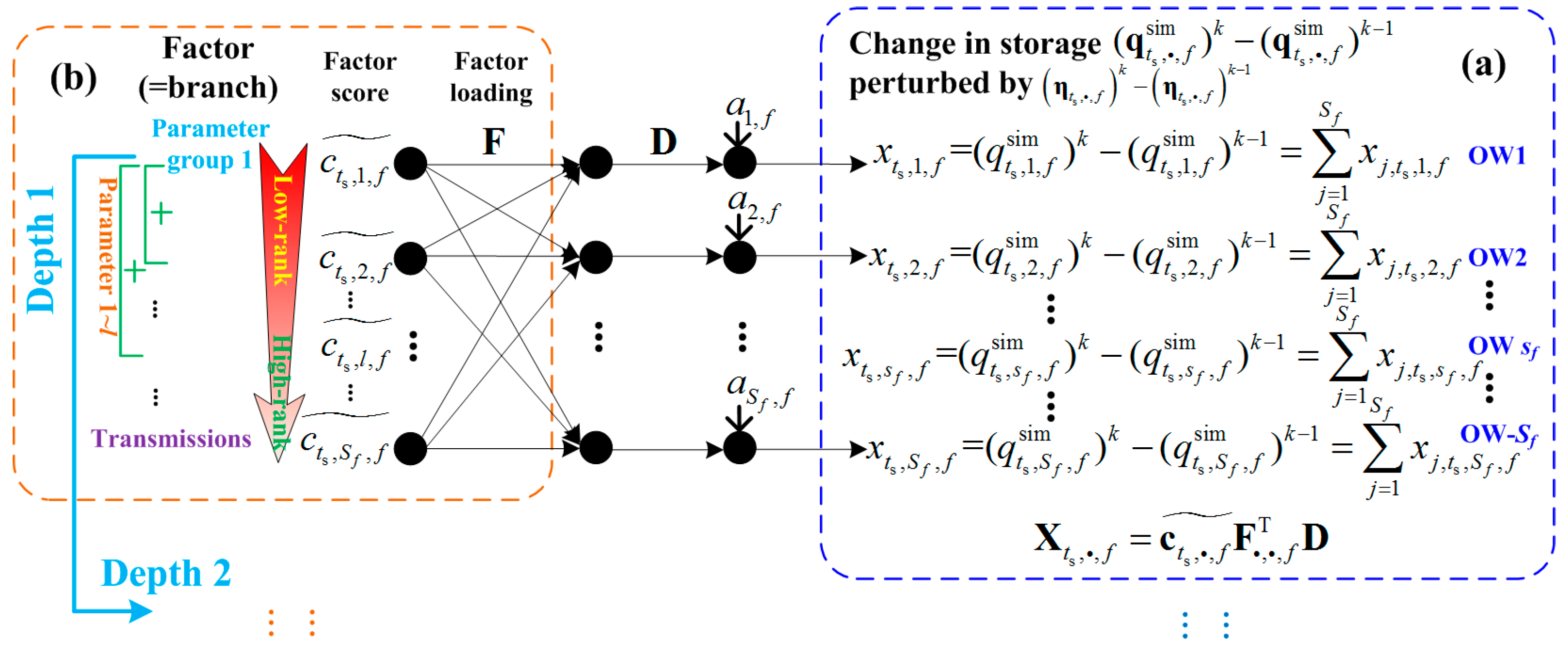
The principal component analysis provides a description model for the simulated spatiotemporal change in storage between the k^th and (k − 1)^th iterations by using SVD. The deviation matrix X can be expressed by the factor score $\tilde{C}$ and the factor loading F as follows:

$$X=U\mathrm{\Sigma }{V}^{\mathrm{T}}=U\mathrm{\Sigma }{V}^{\mathrm{T}}{D}^{-1}D=\sqrt{T_{\mathrm{s}}-1}U{\left(\frac{1}{\sqrt{T_{\mathrm{s}}-1}}{D}^{-1}V\mathrm{\Sigma }\right)}^{\mathrm{T}}D=\tilde{C}{F}^{\mathrm{T}}D$$

(16)

According to the mathematical meaning, the above formula can be interpreted as: there are L independent parameters caused the change in storage following perturbation by ${({\eta }_{t_{\mathrm{s}},s_f,f}^{})}^k-{({\eta }_{t_{\mathrm{s}},s_f,f}^{})}^{k-1}$. The factor score (transpose) matrix ${\tilde{C}}^{\mathrm{T}}=\left[\begin{array}{ccc}\widetilde{c_{1,•,f}}& \cdots & \tilde{c_{T_{\mathrm{s}},•,f}}\end{array}\right]$ stores $T_{\mathrm{s}}$ observations for L factors in aquifer f, where vector $\tilde{c_{t_{\mathrm{s}},•,f}}={\left(\tilde{c_{t_{\mathrm{s}},1,f}},\dots ,\tilde{c_{t_{\mathrm{s}},S_f,f}}\right)}^{\mathrm{T}}$ records the ${\left(t_{\mathrm{s}}\right)}^{\mathrm{th}}$ observation of the S_f factors, as shown in Figure 1.

The signal $\tilde{c_{t_{\mathrm{s}},•,f}}$ (temporal step size) first passes through a mixing process which called the factor loading F (customized spatial direction), where ${\varphi }_{j,s_f,f}$ determines the loading weight (namely, the correlation coefficient) from the l^th parameter’s factor perturbed between the k^th and (k − 1)^th iterations $\widetilde{c_{•,l,f}}$ to the change in storage at ${\left(s_f\right)}^{\mathrm{th}}$ observation well $x_{•,s_f,f}$. Then, L variables pass through the stretching process D (standard deviation) to enlarge or reduce the range of correction values. Finally, shift a again to generate the component of the change in storage between the k^th and (k − 1)^th iterations ${\left(q_{t_{\mathrm{s}},•,f}^{\mathrm{sim}}\right)}^k-{\left(q_{t_{\mathrm{s}},•,f}^{\mathrm{sim}}\right)}^{k-1}$.

3. Numerical Experimental Validation

3.1. Setup of the Test Case

This study uses USGS developed groundwater modeling software ModelMuse v. 3.10 [42] to set up two hypothetic numerical experiments for verification of the proposing parameter identification methodology. The length, width, and height of the designed experimental groundwater system are 2000 × 1000 × 20 m, and the grid specifies the number of columns and row from the top view is 20 × 10 and the width of each column and row is 100 m, as shown in Figure 2. The magnitude of the hypothetical actual parameter values is set according to the alluvial order from southeast to northwest that the set values are described in supplementary materials Section 1, and the layer type is set as convertible.

3.2. Results and Discussion of the Experimental Verification

3.2.1. Experiment 1—Identification of a Single Type of Parameter

The descent footprint of the objective function of Experiment 1 is illustrated in Figure 3a. Results show that the objective function of the three tested algorithms all can successfully descend to search for an optimum value, in which the LMA can descend more rapidly than the SR1 VLS quasi-Newton algorithm and the Jacobian quasi-Newton. However, the SR1 VLS quasi-Newton identifies more accurate parameter values in five of the six zonal parameters, as shown in Figure 4. The identified error percentage of the Jacobian quasi-Newton at iteration five across multiple zonal hydraulic conductivity ranges from 0.18% to 3.75% with an average of 2.39%, those of LMA range from 0.15% to 3.50% with an average of 1.78%, and those of the SR1 VLS quasi-Newton range from 0.09% to 2.65% with an average of 0.76%. Moreover, the VLS quasi-Newton algorithm only made 25 number of transient simulation times among five iterations for calculation of the Hessian matrix and step sizes, but that of the Jacobian quasi-Newton and LMA requires 39 number of simulation times for calculation. Hence, the VLS quasi-Newton only needs 63.64% of simulation times comparing to the Jacobian quasi-Newton and LMA in a six-zonal parameter system to achieve and converge to an optimum. The detailed optimization process and discussion of Experiment 1 are described in Section 2 of the Supplementary Materials.

3.2.2. Experiment 2—Identification of Multiple Types of Parameters Simultaneously

The descent footprint of the objective function of Experiment 2 is illustrated in Figure 3b. Results show that the objective function of the three tested algorithms all can successfully descend at a quadratic convergence rate to search for an optimum, although the SR3 VLS quasi-Newton algorithm with partial aid of SR1 VLS structure descends more slowly than the Jacobian quasi-Newton before iteration 3 and descends more rapidly than LMA. However, the SR3 VLS quasi-Newton iteratively can identify more precise values for hydraulic conductivity, surface recharge, and boundary recharge, as shown in Figure 5a–c, respectively. As the step size of the LMA and Jacobian quasi-Newton is a scalar, the parameter correction vector tends towards highly sensitive surface recharges. The average identified error percentages of the Jacobian quasi-Newton, LMA and the SR3 VLS quasi-Newton at iteration five across multiple zonal hydraulic conductivities are 6.79%, 53.13%, and 0.04%, respectively; those across multiple surfaces recharges are 1.75%, 5.76%, and 0.09%, and those across multiple boundary recharges are 20.62%, 52.31%, and 0.08%. This demonstrates that the set objective functions (LSE of groundwater storage) accompanied by the high–low factor loading scores for direction calculation, which is corrected/enlarged/scaled by the vectorized switchable step sizes, can detect the area of multiple minima, approach the global optimum, and prevent the ill-posed problem. Moreover, the average error of hydraulic conductivity identified by the Jacobian quasi-Newton between Experiment 2 and Experiment 1 rises 4.40%, while Experiment 2 increases twelve parameters over Experiment 1, indicating that the ill-posed occurrence risk rises when the total number of parameters increases. The detailed optimization process, the number of transient simulation times, and discussion of Experiment 2 are described in supplementary materials Section 3.

4. Practical Application

4.1. Study Area

The basin area of the Cho-Shui River alluvial fan which locates at the middle-west of Taiwan is 2079 km². According to terrain, geology, and stratigraphy, the Cho-Shui River alluvial fan can be divided into the apex, middle, and distal fans, as shown in Figure 6a. The aquifer stratification in the alluvial fan is shown in Figure 6b. It shows that rainfall, river, and irrigation water recharge the groundwater system through the unconfined aquifer at the fan apex and that the groundwater then flows west to the coast. The groundwater system in the alluvial fan is approximately 330 m thick, which can be divided into four aquifers and three aquitards. The specific yield (S_y) of the unconfined aquifer at the apex of the fan is 0.137 to 0.237, and the storage coefficient of the confined aquifer varies from 10⁻⁴ to 10⁻³ [16]. Accordingly, the constructed conceptual groundwater flow model of the Cho-Shui River alluvial fan using MODFLOW-2005 is shown in Figure 6c.

4.2. Calibration Outcome and Discussion of the Mega-Parameters Variables of Groundwater Flow Modeling

According to the Cho-Shui River alluvial fan monitoring wells from F1 to F4, the number of Voronoi parameter variable partitions were set to 30, 49, 31, and 16, respectively, with a total of 126 parameter partitions across four aquifers. Therefore, the aquifer hydraulic conductivity, $K_{s_f,f}^{\mathrm{aqu},k}$, has 126 parameters from F1 to F4, with the initial value of $K_{s_f,f}^{\mathrm{aqu},k}$ set by the in situ pumping test. There were six parameters for riverbed conductivity, $K_{{\tau }_{\gamma },\gamma }^{\mathrm{riv},k}$, with the initial value of $K_{{\tau }_{\gamma },\gamma }^{\mathrm{riv},k}$ set by the in situ investigated geological formation. Moreover, there were 96 parameters for aquitard leakance conductivities $K_{s_f,f}^{\mathrm{V},k}$ from T1 to T3, with the initial value of $K_{s_f,f}^{\mathrm{V},k}$ calculated using $K_{zz}$ and the thickness of the aquifer [2]. There were 36 intervals (= 12 months × 3 years) in time, leading to 1080 (=30 × 36) surface parameters that needed identifying. The arc number of recharge across the boundary (=8) was set from F1 to F4, leading to 1152 (= 8 × 4 × 36) parameters. Hence, the entire groundwater flow model for the Cho-Shui River alluvial fan had 2454 parameters to be estimated (126 + 96 + 1080 + 1152 = 2454).

4.2.1. Calculated Results and Discussion of Spatiotemporal Pumpage During 2012–2014

Taiwan Power Company investigated the spatial distribution of pumping wells and recorded the electricity usage for all wells in the Cho-Shui River alluvial fan since 2000. The water usage goals are divided into irrigation wells and non-irrigation wells, with only 610 wells having water rights, while the number of private wells is up to 155,324. The spatial distribution is shown in Figure 6a. Results show that the annual pumpage for irrigation during 2012–2014 was 16.54 × 10⁸, 15.67 × 10⁸, and 15.80 × 10⁸ m³, in consecutive years, while that for non-irrigation was 7.72 × 10⁸, 7.99 × 10⁸, and 7.46 × 10⁸ m³, respectively. The annual total pumpage was 23.73 × 10⁸ m³, of which irrigation pumpage accounted for 67.4% of the total.

Figure 7 illustrates the spatial pattern of the month with maximum pumpage (sub-figures (a), (d), and (h)), the month with minimum pumpage (sub-figures (c), (f), and (i)), and the month closest to the median (sub-figures (c), (f), and (i)) during 2012–2014. Results show that the maximum pumpage in 2012 and 2013 (2.09 × 10⁸ and 2.13 × 10⁸ m³) was in March (at the end of the dry season) and February (starting the mixed cultivation period of paddy and dry farming). Because of large water demand and insufficient surface water supply, the water sources for each demand during this month relied mainly on groundwater pumping. Moreover, the minimum pumpage during 2012–2014 (1.33 × 10⁸, 1.54 × 10⁸, and 1.18 × 10⁸ m³) were in November and December, which are the end of the wet season and the dry farming cultivation period, respectively. Moreover, in the unusually dry year in 2014, there was only one typhoon Fung-Wong, which occurred at the end of September to provide rainfall and surface water. Therefore, the maximum pumpage was in August (2.30 × 10⁸ m³), with the pumpage being closest to the mean value in April (2.08 × 10⁸ m³). Overall, high-intensity pumping is mainly concentrated in the distal alluvial fan. During the dry season and the month with high water demand, the high-intensity pumping areas extend to the interior of the middle alluvial fan.

4.2.2. Initially Estimated Spatiotemporal Pattern of Groundwater Recharge

After analyzing the principal components of the monthly spatiotemporal inflow and transmission during 2012–2014, the overlain multi-rank factor loading for initial groundwater recharge spatial allocation in F1, F2, F3, and F4 is from PC1 to PC5, which is determined by practical in situ conditions and the minimal value and maximal objective function gradient, as shown in Figure 8. This figure shows that the recharge in F1 and F2 of the Cho-Shui River alluvial fan has higher loadings in the proximal fan. This is because the lithology in the apex is mostly composed of high permeability gravel, which presents a gradually decreasing trend for permeability from the apex to the tail [16]. Furthermore, the loadings’ spatial pattern in F3 is larger near the northern and eastern regions. This suggests that the recharge source of F3 is mainly from recharge across the boundary, while that from aquitard leakance conductivities is less [36]. The boundary recharge in F4 is mainly distributed in the northeastern region, while the leakage from F3 is mainly concentrated in the middle and distal fans. The above analysis shows that a multi-rank loading combination can initially estimate the general trend of the spatial pattern of surface recharge and boundary recharge.

4.2.3. Calibration Process and Discussion

During the iterative calibration process, the high-rank components for Hessian approximation moved along the corrected direction for surface recharge identification ranging from 2 to 4, with the average of F1, F2, F3, and F4 being 2.37, 2.78, 2.53, and 2.29, respectively. For boundary recharge identification, components ranged from 5 to 9, with the average of F1, F2, F3, and F4 being 6.62, 8.43, 7.29, and 5.37, respectively; and those for hydraulic conductivity identification ranged from 8 to 16, with the average of F1, F2, F3, and F4 being 10.78, 13.61, 11.37, and 9.14, respectively. After 24 iterative calculations, the convergent process of the error descent of each aquifer is shown in Figure 9. After the first iteration, the simulated storage error percentage ($\underset{t_{\mathrm{s}},s_f}{\mathrm{E}}\left[\frac{q_{t_{\mathrm{s}},s_f,f}^{\mathrm{sim}}\left(\mathsf{\eta }\right)-q_{t_{\mathrm{s}},s_f,f}^{\mathrm{obs}}}{q_{t_{\mathrm{s}},s_f,f}^{\mathrm{obs}}}\times 100\%\right]$) of each aquifer in the transient state can be effectively reduced. Before iteration #6, the average error descent rate per iteration from F1 to F4 was −59.73%, −17.10%, −17.62%, and −23.96%, respectively, which illustrates that the vectorized limited step size can effectively accelerate convergence along the corrected direction for each parameter. Because of the complex groundwater recharge mechanism and hydrogeological structure in F1, the initial simulated error percentage was greater than in the other three deep aquifers. After iteration #6, the error percentage of F1 begins to converge, showing a steady decline, which is lower than the other three deep aquifers, with the average error descent rates from F1 to F4 of −0.72%, −0.46%, −0.91%, and −0.87%, respectively. Finally, after 24 iterations, the stopping criterion was met, and the error percentages from F1 to F4 are 0.11%, 23.58%, 28.99%, and 29.55%, respectively. Results showed that due to an insufficient number of groundwater head monitoring wells and low frequency of the pumping test in deep aquifers (F2, F3, and F4), the groundwater budget estimated from groundwater head fluctuation was highly uncertain. Therefore, the error percentage in F2, F3, and F4 are larger than in F1.

4.2.4. Results and Discussions of Identified Parameters

After 24 iterations, the calculated $\underset{t_{\mathrm{s}},s_f}{\mathrm{E}}\left[{\beta }_{t_{\mathrm{s}},s_f,f}^k\right]$ hyetographs across the aquifers are shown for twelve months in Figure 10, where ${\beta }_{t_{\mathrm{s}},s_f,f}^k$ is the ratio between the identified surface recharge and lumped recharge. The ${\beta }_{t_{\mathrm{s}},s_f,f}^k$ values of F1, F2, F3, and F4 in the wet season (April to August) range from 64.3–144.0%, 63.9–88.5%, 63.8–83.8%, and 69.4–86.8% during 2012–2014, respectively, while those in the dry season (September to March) ranged from 21.4–67.2%, 12.8–35.7%, 17.6–35.6%, and 11.4–34.5%, respectively. The ${\beta }_{t_{\mathrm{s}},s_f,f}^k$ value in the dry season is smaller ($\underset{t_{\mathrm{s}},s_f,k}{\mathrm{E}}\left[{\beta }_{t_{\mathrm{s}},s_f,1}^k,{\beta }_{t_{\mathrm{s}},s_f,2}^k,{\beta }_{t_{\mathrm{s}},s_f,3}^k,{\beta }_{t_{\mathrm{s}},s_f,4}^k\right]=[35.5\%,27.0\%,27.0\%,27.3\%]$), showing that the recharge source is mainly from the boundary because of less precipitation [16]. The precipitation during the wet season, when groundwater storage increases, is high, resulting in a larger ${\beta }_{t_{\mathrm{s}},s_f,f}^k$ ($\underset{t_{\mathrm{s}},s_f,k}{\mathrm{E}}\left[{\beta }_{t_{\mathrm{s}},s_f,1}^k,{\beta }_{t_{\mathrm{s}},s_f,2}^k,{\beta }_{t_{\mathrm{s}},s_f,3}^k,{\beta }_{t_{\mathrm{s}},s_f,4}^k\right]=[89.8\%,74.1\%,73.0\%,74.6\%]$). After a large amount of surface water enters into the aquifer, increasing the groundwater head higher than the boundary of the river or sea head, outflow and loss from the groundwater aquifer occurred [16]. Therefore, the ${\beta }_{t_{\mathrm{s}},s_f,f}^k$ of F1 in July and August is greater than 1 ($\underset{s_f,k}{\mathrm{E}}\left[{\beta }_{7,s_f,1}^k,{\beta }_{8,s_f,1}^k\right]=[109.9\%,117.3\%]$), which indicates that the actual recharge is larger than the volume fluctuation in the groundwater head. Furthermore, the deep aquifer recharge sources are the leakage from the shallow aquifers and boundary recharge [36]. Verifiably, due to the lower $K_{t_{\mathrm{s}},s_f}^{\mathrm{aqu}}$ and $K_{t_{\mathrm{s}},s_f}^{\mathrm{V}}$ in the aquitard, the leaking recharge efficiency is poor than the boundary recharge, resulting in the average $\underset{t_{\mathrm{s}},s_f,k}{\mathrm{E}}\left[{\beta }_{t_{\mathrm{s}},s_f,2}^k,{\beta }_{t_{\mathrm{s}},s_f,3}^k,{\beta }_{t_{\mathrm{s}},s_f,4}^k\right]$ only reaching 46.6%, 46.2%, and 47.0%, respectively, which are less than 50%.

Figure 11 illustrates the identified surface recharge spatial pattern of Aquifer 1 and leakance conductivities of Aquitards 1, 2, and 3. Results show that surface recharge and aquitard leakance conductivities across aquifers in the Chou-Shui River alluvial fan are most active in the proximal fan [36] (area percentage subject to surface recharge on F1 > 0.02 m/d = 87.2%, and area percentage subject to aquitard leakance conductivities on F2, F3, and F4 > 0.002 1/d = [93.6%,71.2%,84.5%]. The geological broken belt in the middle fan is the second-highest recharge region. Additionally, the identified spatial pattern of $K_{t_{\mathrm{s}},s_f}^{\mathrm{aqu}}$ is shown in Figure 12. Results illustrate that the $K_{t_{\mathrm{s}},s_f}^{\mathrm{aqu}}$ patterns of F1 and F4 are consistent with the river’s alluvial order from upstream to downstream, while those of F2 and F3 show a highly non-homogeneous and non-isotropic pattern due to multiple transgressions and regressions [16].

Figure 13 illustrates the spatial pattern of root mean square error (RMSE) between simulated and observed groundwater heads across multiple aquifers in the Cho-Shui River alluvial fan. The average groundwater head RMSE of F1, F2, F3, and F4 is 0.134 m, 0.677 m, 0.708 m, and 0.916 m, respectively. Results show that the simulated groundwater head accuracy of F1 is better than that of F2, F3, and F4, because of the high uncertainty in the hydrogeological structure of the deep aquifer. However, the correlation coefficient of F2, F3, and F4 can reach 0.659, 0.544, and 0.609, respectively, allowing the simulated hydrograph to capture the groundwater head fluctuation trend. The above-identified and simulated results illustrate that the rank three combined high–low-rank factor loading scores analyzed from the simulated storage fluctuation between adjacent iterations for the Hessian approximation not only can reduce the computation efforts but also can converge to the global minimum solution subject to the true in situ hydrogeology. The areas with larger RMSE in F1 are mainly distributed in the apex and part of the distal fan because the monitoring, estimation, and simulation of boundary recharge are difficult.

The comparisons among the simulated and observed groundwater head hydrographs across multiple aquifers are illustrated in Figure 14, in which MT station (Figure 14a), TK station (Figure 14b), and TH station (Figure 14c) are located in the distal fan, middle fan, and proximal fan, respectively. Results illustrate that the RMSEs of Aquifer 2 (Figure 14-2) in stations MT, TK, and TH are as large as 3.78, 7.40, and 3.67 times that of Aquifer 1 (Figure 14-1), respectively; and those of Aquifer 3 (Figure 14-3) is as large as 4.67, 3.60, and 4.87 times that of Aquifer 1 (Figure 14-1), showing that the confined aquifer with insufficient monitoring network (e.g., middle fan of Aquifer 2 and proximal fan of Aquifer 3) would be hard to detect the actual flow condition and reduce the identified accuracy in groundwater head and parameters. From Figure 14-4 which illustrates the quartile analysis of the simulated error across multiple aquifers, this study discovers that the groundwater head at Aquifer 1 across all sub-fans can achieve closely full fitting in groundwater head. However, the transient simulated errors at Aquifers 2 and 3 increase in which the standard deviation is 1.26m and 0.88m in MT station, respectively; that is 1.52m and 0.92m in TK station, and that is 0.61m and 1.83m in TH station. Hence, this study discovers that the exchange and flow mechanism in distal and middle fan at Aquifer 2 is more complex than that at Aquifer 3; Contrarily, the mechanisms in the proximal fan at Aquifer 3 is more complex than Aquifer 2. The current monitoring network is incapable to detect the full inflow, outflow, and groundwater flow accurately at Aquifers 2 and 3.

5. Conclusions and Suggestion

In a multi-layered complex groundwater model, achieving accurate spatiotemporal identification for different kinds of parameters and solving the ill-posed problem is the vital research topic in model calibration. This study proposes an SR3 VLS quasi-Newton algorithm by modifying the Levenberg–Marquardt algorithm and importing a rank three structure from the Broyden–Fletcher–Goldfarb–Shanno algorithm to solve the constrained identification of hydrogeological parameters and spatiotemporal recharge patterns simultaneously associated with an iterative approach in a large-scale multi-layered groundwater model. The recharge parameters include surface and boundary recharge, and the hydrogeological parameters consist of riverbed leakage, aquifer hydraulic, and aquitard leakance conductivities. To accelerate directional convergence, approach a global optimum, and achieve a well-posed problem, this study uses a vectorized limited switchable step size in the inverse problem of transmissive groundwater. Accordingly, to achieve the Hessian approximation, solve nonlinear ill-posed problems, and detect the global minimum area, this study imports a rank three structure, which uses a high-rank and a low-rank factor loading score analyzed from the simulated storage difference between two adjacent iterations to calculate the correction matrix for the Hessian. Moreover, it modifies the traditional algorithm from the scalar line search to vectorized multi-order derivative exact double false position bracketing using SVD-related rank and depth information for solving the vectorized step size corresponding to different hydrogeological parameters and recharges. The proposing methodology is verified by numerical experiments and is applied in a complex practical multi-layered groundwater system.

This study designed two numerical experiments to verify the capability of identifying multiple parameters and recharges through the proposing modified algorithm. Experiment 1 identified six zonal hydraulic conductivities, using a single factor loading score to approximate the Hessian. Except for six hydraulic conductivities, the parameters to be identified in Experiment 2 increased six surfaces recharges and six boundaries recharges that uses overlaid high–low factor loading scores. Results show that the iteratively objective function footprint of the three tested quasi-Newton algorithms (Jacobian, LMA, and SR3 VLS) all successfully descend at a quadratic convergence rate to search for an optimum. The identified average error percentage of the Jacobian quasi-Newton, LMA, and the SR3 VLS quasi-Newton algorithm across multiple zonal hydraulic conductivities in Experiment 1 are 2.39%, 1.78%, and 0.76%, respectively; and those across multiple surfaces recharges in Experiment 2 are 1.75%, 5.76%, and 0.09%. This demonstrates that the set objective function (LSE of groundwater storage) and the high–low combination of factor loading scores employed can detect the exact global minimum area, in which the vectorized limited switchable step sizes were striving to accelerate convergence along the corrected direction to leap from local optimum and approach a global optimum iteratively. Hence, the identified parameters by using the SR3 VLS quasi-Newton can converge to the true solution by solving nonlinear ill-posed problems. Moreover, the adopted PC Rank Depth pattern for identification illustrates that surface recharge is the largest and most direct factor affecting the fluctuation of groundwater storage with shorter travel times, and boundary recharge greatly influences the storage fluctuations with longer response lag time.

The established method was applied to the groundwater system of the Chou-Shui River alluvial fan in Taiwan. The simulated period is from January 2012 to December 2014. Results show that the RMSE during the calibration process can quickly converge in six iterations, with a decreased rate of −59.73%, −17.10%, −17.62%, and −23.96%, by considering the transmissive flow differences between single perturbation and multiple corrections of parameters simultaneously. Moreover, the average simulated storage error percentage of aquifer 1 is as small as 0.11%, with an RMSE of 0.134 m. This shows that the developed methodology not only validly detects the flow tendency and error source to quantify the spatiotemporal correction values but also precisely simulates the peak and fluctuation in groundwater head.

While calculating the multi-rank factor loading score analyzed from the simulated storage difference using SVD, if the monitoring well pattern is poor or overdense, the decomposed high–low loading scores for the rank three Hessian approximate may be far away from the real matrix. To achieve accurate and beneficial identification of parameters, optimal monitoring network design is the source of performance limitation of the developed SR3 VLS algorithm.

References

1. Abdi, R.; Endrney, T.; Nowak, D. A model to integrate urban river thermal cooling in river restoration. J. Environ. Manag. 2020, 258, 110023. [Google Scholar] [CrossRef] [PubMed]
2. McDonald, M.G.; Harbaugh, A.W. A Modular Three-Dimensional Finite-Difference Ground-Water Flow Model; USGPO: Washington, DC, USA, 1988.
3. Neuman, S.P. Calibration of distributed parameter groundwater flow models viewed as a multiple-objective decision process under uncertainty. Water Resour. Res. 1973, 9, 1006–1021. [Google Scholar] [CrossRef]
4. Christiansen, L.; Binning, P.J.; Rosbjerg, D.; Andersen, O.B.; Bauer-Gottwein, P. Using time-lapse gravity for groundwater model calibration: An application to alluvial aquifer storage. Water Resour. Res. 2011, 47, 12. [Google Scholar] [CrossRef] [Green Version]
5. Hsu, N.-S.; Yeh, W.W.G. Optimum experimental design for parameter identification in groundwater hydrology. Water Resour. Res. 1989, 25, 1025–1040. [Google Scholar] [CrossRef]
6. LaVenue, A.M.; Pickens, J.F. Application of a coupled adjoint sensitivity and kriging approach to calibrate a groundwater flow model. Water Resour. Res. 1992, 28, 1543–1569. [Google Scholar] [CrossRef]
7. Małloszewski, P.; Zuber, A. On the calibration and validation of mathematical models for the interpretation of tracer experiments in groundwater. Adv. Water Resour. 1992, 15, 47–62. [Google Scholar] [CrossRef]
8. Poeter, E.P.; Hill, M.C. Inverse models: A necessary next step in ground-water modeling. Groundwater 1997, 35, 250–260. [Google Scholar] [CrossRef]
9. Hill, M.C.; Cooley, R.L.; Pollock, D.W. A controlled experiment in ground water flow model calibration. Groundwater 1998, 36, 520–535. [Google Scholar] [CrossRef]
10. Solomatine, D.; Dibike, Y.; Kukuric, N. Automatic calibration of groundwater models using global optimization techniques. Hydrol. Sci. J. 1999, 44, 879–894. [Google Scholar] [CrossRef] [Green Version]
11. Sonnenborg, T.O.; Christensen, B.S.; Nyegaard, P.; Henriksen, H.J.; Refsgaard, J.C. Transient modeling of regional groundwater flow using parameter estimates from steady-state automatic calibration. J. Hydrol. 2003, 273, 188–204. [Google Scholar] [CrossRef]
12. Doherty, J. Ground water model calibration using pilot points and regularization. Groundwater 2003, 41, 170–177. [Google Scholar] [CrossRef] [PubMed]
13. Hendricks Franssen, H.; Kinzelbach, W. Real-time groundwater flow modeling with the ensemble kalman filter: Joint estimation of states and parameters and the filter inbreeding problem. Water Resour. Res. 2008, 44, W09408. [Google Scholar] [CrossRef]
14. Du, X.; Lu, X.; Hou, J.; Ye, X. Improving the reliability of numerical groundwater modeling in a data-sparse region. Water 2018, 10, 289. [Google Scholar] [CrossRef] [Green Version]
15. Cheng, Q.-B.; Chen, X.; Cheng, D.-D.; Wu, Y.-Y.; Xie, Y.-Y. Improved inverse modeling by separating model structural and observational errors. Water 2018, 10, 1151. [Google Scholar] [CrossRef] [Green Version]
16. Hsu, N.-S.; Chiang, C.-J.; Wang, C.-H.; Liu, C.-W.; Huang, C.-L.; Liu, H.-J. Estimation of pumpage and recharge in alluvial fan topography under multiple irrigation practices. J. Hydrol. 2013, 479, 35–50. [Google Scholar] [CrossRef]
17. Nocedal, J.; Wright, S. Numerical Optimization; Springer: New York, NY, USA, 2006. [Google Scholar]
18. Floudas, C.A.; Pardalos, P.M. Encyclopedia of Optimization; Springer US: New York, NY, USA, 2008. [Google Scholar]
19. Mittelhammer, R.C.; Judge, G.G.; Miller, D.J. Econometric Foundations Pack with CD-ROM; Cambridge University Press: Cambridge, UK, 2000. [Google Scholar]
20. Kanzow, C.; Yamashita, N.; Fukushima, M. Levenberg-Marquardt methods with strong local convergence properties for solving nonlinear equations with convex constraints. J. Comput. Appl. Math. 2005, 173, 321–343. [Google Scholar] [CrossRef] [Green Version]
21. Curtis, F.E.; Que, X.C. A quasi-newton algorithm for nonconvex, nonsmooth optimization with global convergence guarantees. Math. Program. Comput. 2015, 7, 399–428. [Google Scholar] [CrossRef]
22. Dahlquist, G.; Björck, Å. Numerical Methods; Dover Publications: Mineola, NY, USA, 2003. [Google Scholar]
23. Tung, C.P.; Chou, C.A. Pattern classification using tabu search to identify the spatial distribution of groundwater pumping. Hydrogeol. J. 2004, 12, 488–496. [Google Scholar] [CrossRef]
24. Tsai, F.T.C.; Yeh, W.W.G. Characterization and identification of aquifer heterogeneity with generalized parameterization and bayesian estimation. Water Resour. Res. 2004, 40, 12. [Google Scholar] [CrossRef] [Green Version]
25. Cheng, W.C.; Kendall, D.R.; Putti, M.; Yeh, W.W.G. A nudging data assimilation algorithm for the identification of groundwater pumping. Water Resour. Res. 2009, 45, 13. [Google Scholar] [CrossRef]
26. Liu, H.J.; Hsu, N.S.; Lee, T.H. Simultaneous identification of parameter, initial condition, and boundary condition in groundwater modelling. Hydrol. Process. 2009, 23, 2358–2367. [Google Scholar] [CrossRef]
27. Liu, H.J.; Hsu, N.S. Novel information for source identification of local pumping and recharging in a groundwater system. Hydrol. Sci. J. 2015, 60, 723–735. [Google Scholar] [CrossRef]
28. Liu, H.J.; Hsu, N.S.; Yeh, W.W.G. Independent component analysis for characterization and quantification of regional groundwater pumping. J. Hydrol. 2015, 527, 505–516. [Google Scholar] [CrossRef]
29. Cuthbert, M.O.; Acworth, R.I.; Andersen, M.S.; Larsen, J.R.; McCallum, A.M.; Rau, G.C.; Tellam, J.H. Understanding and quantifying focused, indirect groundwater recharge from ephemeral streams using water table fluctuations. Water Resour. Res. 2016, 52, 827–840. [Google Scholar] [CrossRef]
30. Wittenberg, H.; Sivapalan, M. Watershed groundwater balance estimation using streamflow recession analysis and baseflow separation. J. Hydrol. 1999, 219, 20–33. [Google Scholar] [CrossRef]
31. Arnold, J.G.; Muttiah, R.S.; Srinivasan, R.; Allen, P.M. Regional estimation of base flow and groundwater recharge in the upper Mississippi river basin. J. Hydrol. 2000, 227, 21–40. [Google Scholar] [CrossRef]
32. Healy, R.W.; Cook, P.G. Using groundwater levels to estimate recharge. Hydrogeol. J. 2002, 10, 91–109. [Google Scholar] [CrossRef]
33. Moon, S.-K.; Woo, N.C.; Lee, K.S. Statistical analysis of hydrographs and water-table fluctuation to estimate groundwater recharge. J. Hydrol. 2004, 292, 198–209. [Google Scholar] [CrossRef]
34. Lee, C.-H.; Yeh, H.-F.; Chen, J.-F. Estimation of groundwater recharge using the soil moisture budget method and the base-flow model. Environ. Geol. 2008, 54, 1787–1797. [Google Scholar] [CrossRef]
35. Martínez-Santos, P.; Martínez-Alfaro, P. Estimating groundwater withdrawals in areas of intensive agricultural pumping in central Spain. Agric. Water Manag. 2010, 98, 172–181. [Google Scholar] [CrossRef]
36. Yu, H.-L.; Chu, H.-J. Understanding space–time patterns of groundwater system by empirical orthogonal functions: A case study in the Choshu River alluvial fan, Taiwan. J. Hydrol. 2010, 381, 239–247. [Google Scholar] [CrossRef]
37. Yeh, W.W.-G. Review: Optimization methods for groundwater modeling and management. Hydrogeol. J. 2015, 23, 1051–1065. [Google Scholar] [CrossRef]
38. Cooley, R.L. A method of estimating parameters and assessing reliability for models of steady state groundwater flow: 1. Theory and numerical properties. Water Resour. Res. 1977, 13, 318–324. [Google Scholar] [CrossRef]
39. Carrera, J.; Neuman, S.P. Estimation of aquifer parameters under transient and steady state conditions: 1. Maximum likelihood method incorporating prior information. Water Resour. Res. 1986, 22, 199–210. [Google Scholar] [CrossRef]
40. Fletcher, R. Practical Methods of Optimization; Wiley: Hoboken, NJ, USA, 2013. [Google Scholar]
41. Hayley, K.; Valenza, A.; White, E.; Hutchison, B.; Schumacher, J. Application of the iterative ensemble smoother method and cloud computing: A groundwater modeling case study. Water 2019, 11, 1649. [Google Scholar] [CrossRef] [Green Version]
42. Winston, R.B. Modelmuse—A graphical user interface for MODFLOW-2005 and PHAST. In U.S. Geological Survey Techniques and Methods; USGS: Reston, VA, USA, 2009. [Google Scholar]
Figure 1. Schematic diagram of singular value decomposition of changes in storage between the kth and (k − 1)th iterations with once simulation perturbation: (a) observed change in storage ( q t s , , f sim ) k ( q t s , , f sim ) k 1 ; (b) decomposed components of change in storage perturbed by the correction in the parameter ( η t s , , f ) k ( η t s , , f ) k 1 .
Water 12 00995 g001
Figure 2. Overview of the numerical experiment area.
Water 12 00995 g002
Figure 3. Comparison of descent footprint of objective function: (a) Experiment 1; (b) Experiment 2.
Water 12 00995 g003
Figure 4. Error percentage of identified hydraulic conductivity using Jacobian quasi-Newton, LMA, and SR1 VLS quasi-Newton algorithms during iterations across multiple zones in Experiment 1.
Water 12 00995 g004
Figure 5. Error percentage of identified hydraulic conductivity (a), surface recharge (b) and boundary recharge (c) during iterations across multiple zones in Experiment 2.
Water 12 00995 g005
Figure 6. Study area: (a) distribution of groundwater monitoring wells, pumping wells, and sub-alluvial fan; (b) aquifer/aquitard stratification profile across all drilling wells; (c) constructed hydrogeological gridding structure of groundwater modeling.
Water 12 00995 g006
Figure 7. Calculated monthly pumpage of Cho-Shui River alluvial fan during 2012–2014.
Water 12 00995 g007
Figure 8. The overlaid factor loadings for an initial spatial estimate of surface/boundary recharge in Cho-Shui River alluvial fan: (a) Aquifer 1; (b) Aquifer 2; (c) Aquifer 3; (d) Aquifer 4.
Water 12 00995 g008
Figure 9. Simulated storage error percentages vs. number of iterations for the Chou-Shui River alluvial fan groundwater system.
Water 12 00995 g009
Figure 10. The calculated E s f , k [ β t s , s f , f k ] hyetograph across four aquifers.
Water 12 00995 g010
Figure 11. The identified spatial pattern of surface recharge R t s , s 1 surf and aquitard leakance conductivities K s f , f V : (a) Aquifer 1; (b) Aquitard 1; (c) Aquitard 2; and (d) Aquitard 3.
Water 12 00995 g011
Figure 12. The identified spatial pattern of aquifer’s hydraulic conductivity K s f , f aqu : (a) Aquifer 1; (b) Aquifer 2; (c) Aquifer 3; and (d) Aquifer 4.
Water 12 00995 g012
Figure 13. The spatial pattern of root mean square error (RMSE) between simulated and observed groundwater heads: (a) Aquifer 1; (b) Aquifer 2; (c) Aquifer 3; and (d) Aquifer 4.
Water 12 00995 g013
Figure 14. Comparison among simulated and observed groundwater head hydrographs: (a) MT station; (b) TK station; (c) TH station; (-1) Aquifer 1; (-2) Aquifer 2; (-3) Aquifer 3; and (-4) quartile analysis of simulated error.
Water 12 00995 g014