Article

Effects of Transverse Groynes on Meso-Habitat Suitability for Native Fish Species on a Regulated By-Passed Large River: A Case Study along the Rhine River

1
CNRS UMR 7362 LIVE, University of Strasbourg, F-67083 Strasbourg, France
2
CNRS UMR 5600 EVS, University of Lyon, Site ENS, F-69362 Lyon, France
3
Ecole Nationale du Génie de L’eau et de L’environnement de Strasbourg (ENGEES), École D’ingénieurs—Eau et Environnement, F-67000 Strasbourg, France
4
Électricité de France (EDF), Centre d’Ingénieurie Hydraulique (CIH), F-73370 Le Bourget-du-Lac, France
*
Author to whom correspondence should be addressed.
Water 2020, 12(4), 987; https://doi.org/10.3390/w12040987
Submission received: 28 February 2020 / Revised: 18 March 2020 / Accepted: 23 March 2020 / Published: 31 March 2020
(This article belongs to the Section Water Quality and Contamination)

Abstract

:
River regulations ultimately degrade fluvial forms and morphodynamics and simplify riparian and aquatic habitats. For several decades, river restoration actions have been performed to recover geomorphic processes and diversify these habitats to enhance both river biodiversity and ecosystem services. The objective of this study is to provide quantitative feedback on the experimental restoration of a large regulated and by-passed river (the Upper Rhine downstream of the Kembs Dam, France/Germany). This restoration consisted of the construction of two transverse groynes and the removal of bank protection. A monitoring framework composed of topo-bathymetric surveys as well as flow velocity and grain size measurements was established to assess the channel morphodynamic responses and evaluate their effects on habitat suitability for five native fish species using habitat models. A riverscape approach was used to evaluate the landscape changes in terms of both the configuration and the composition, which cannot be considered with classic approaches (e.g., Weighted Usable Area). Our results show that the two transverse groynes and, to a lesser extent, bank erosion, which was locally enhanced by the two groynes, increased habitat diversity due to the creation of new macroforms (e.g., pools and mid-bars) and fining of the bed grain size. Using a riverscape approach, our findings highlight that the restoration improved eel and juvenile nase species due to slowing down of the current and the deposition of fine sediments downstream of both groynes. As a consequence, the restoration improved the habitat suitability of the studied reach for more fish species compared with the pre-restoration conditions. This study also demonstrates that the salmon habitats downstream of the restored reach were improved due to fining of the bed grain size. This finding highlights that, for restorations aimed at fish habitats, the grain size conditions must be taken into consideration along with the flow conditions. Furthermore, the implementation of groynes, while not a panacea in terms of functional restoration, can be a strategy for improving fish habitats on highly regulated rivers, but only when more functional and natural options are impossible due to major constraints.

1. Introduction

Most large rivers have been regulated for the purposes of flood protection, navigation, and agricultural development, as well as electricity production. However, these regulations have induced the degradation of both geomorphological and hydrological conditions (e.g., the fragmentation of river networks and a deficit of sediment) [1,2]. As a result, river habitats have been heavily disturbed, altering aquatic and riverine communities and biodiversity [3,4].
Over the past several decades, an increasing number of river restorations has been undertaken, notably in Europe, where this rise in restoration programs has been fostered by the European Water Framework Directive (WFD) [5]. The main objective of such restoration actions is to improve the functional processes of rivers and thus recover ecosystem services [6,7,8,9,10]. River restoration actions can be implemented for one or more of the seven following categories: continuity restoration, pollution control, recovery of sediment dynamics, land-use management, adaptation to climate change, implementation of ecological discharges, and habitat restoration [11].
Numerous restorations targeted the recovering habitats of some native fish species due to their emblematic value and habitat requirements. For example, since the 1960s, restorations of rivers in California, USA were performed to recover spawning areas for salmon by using gravel augmentations, which were sometimes combined with artificial riffles [12]. Either fish passes were launched or low dams were removed to restore river continuity [13]. More recently, several engineering strategies were tested along the Danube River, such as (i) riprap removal and groyne shortening, (ii) riprap and groyne field removal, and (iii) side channel reconnection, to increase the abundance of rheophilic fishes [14]. Historically, groynes were structures composed by wood and/or rocks and used to promote bed erosion in the main channel and maintain a minimum water level for navigation purposes [15]. Recently, longitudinal training dams (LTDs) were tested along the Rhine river to simultaneously improve navigation during low flows, enhance safety for human activities and hydraulic infrastructures against floods, and create refugia for native fish at their juvenile stages [16]. On the channelized Godwin Creek River, stones were added to extend 18 small groynes to promote channel diversification and enhance fish habitats [17]; this research highlighted that the extension of groynes promoted habitat heterogeneity by increasing pool habitats and promoting grain size fining, following which the composition and relative abundance of fish were similar to those of the non-incised reference site. Lacey and Millar [18] in their research used hydrodynamic models on the Chiliwack River to assess the effect of large wood within the stream and the implementation of rock groyne habitat structures (both simple and double rock groynes); their modeling results showed that these actions promoted an increase in habitat suitability for two salmonids (Oncorhynchus kisutch, Oncorhynchus mykiss) during high flows. Fish species can be viewed as umbrella species, i.e., species whose conservation is expected to confer protection to a large number of naturally co-occurring species [19]. Hence, a restoration implemented for a native fish community is usually good for the whole ecosystem. Fish react promptly to human modifications of an ecosystem and thus can be used as indicators of river recovery and, more broadly, the ecological status of waterbodies [20,21]. Thorough knowledge of the biology of fish species and the requirements for those species to complete their life cycle makes it possible to predict which habitats will be able to host a given species or a given functional category of fish. Consequently, fish habitat models are frequently employed to determine minimal in-stream discharges to improve the habitat suitability for native fish species on by-passed reaches [22,23,24], to assess habitat changes induced by hydropeaking or weir and reservoir removal [25], and to evaluate the effects of restoration actions [26,27]. The most commonly used modeling method is the in-stream flow incremental methodology (IFIM) developed by the U.S. Fish and Wildlife Service during the 1970s [28]. This methodology evaluates habitat suitability through the habitat suitability index (HSI), derived from fish species preferences and related to numerous environmental variables (e.g., water depth, flow velocity, and grain size of the bed substrate) [20,29,30,31].
Most fish habitat models are based on quantitative estimations of habitat suitability using micro-habitat approaches. However, the composition and configuration of riverscape units and the associated meso-habitats at a larger scale are rarely taken into account, although ecological processes at the population and community levels are affected by these factors [32]. The use of a meso-habitat rather than a micro-habitat approach allows these changes to be quantified [33] and is potentially useful for detecting riverscape changes following natural or human disturbances [34]. Based on this approach, a new ecological hydrograph relating flow to habitat quality for Spinibarbus hollandi on the Lijiang River was proposed by Li et al. [33]. The advantage of using the riverscape approach rather than the micro-scale approach to assess the effects of low dams on fish habitat quality was shown on the Neosho River by Hitchman et al. [34].
A riverscape approach was used to quantitatively assess the effects of channel restoration based on the implementation of two transverse groynes on habitat diversification and a rise in potential fish abundance using riverscape metrics. Two hypotheses were tested: (i) the restoration action promoted the diversification of aquatic habitats, and (ii) the diversification of aquatic habitats improved the habitat suitability for the native fish studied. Geomorphological monitoring based on a before-after-control-impact (BACI) design [35] was achieved to evaluate the channel responses following the restoration, allowing us to calibrate two-dimensional hydraulic models to build fish habitat models for five native species based on empirical preferences determined along French rivers [36,37].

2. Materials and Methods
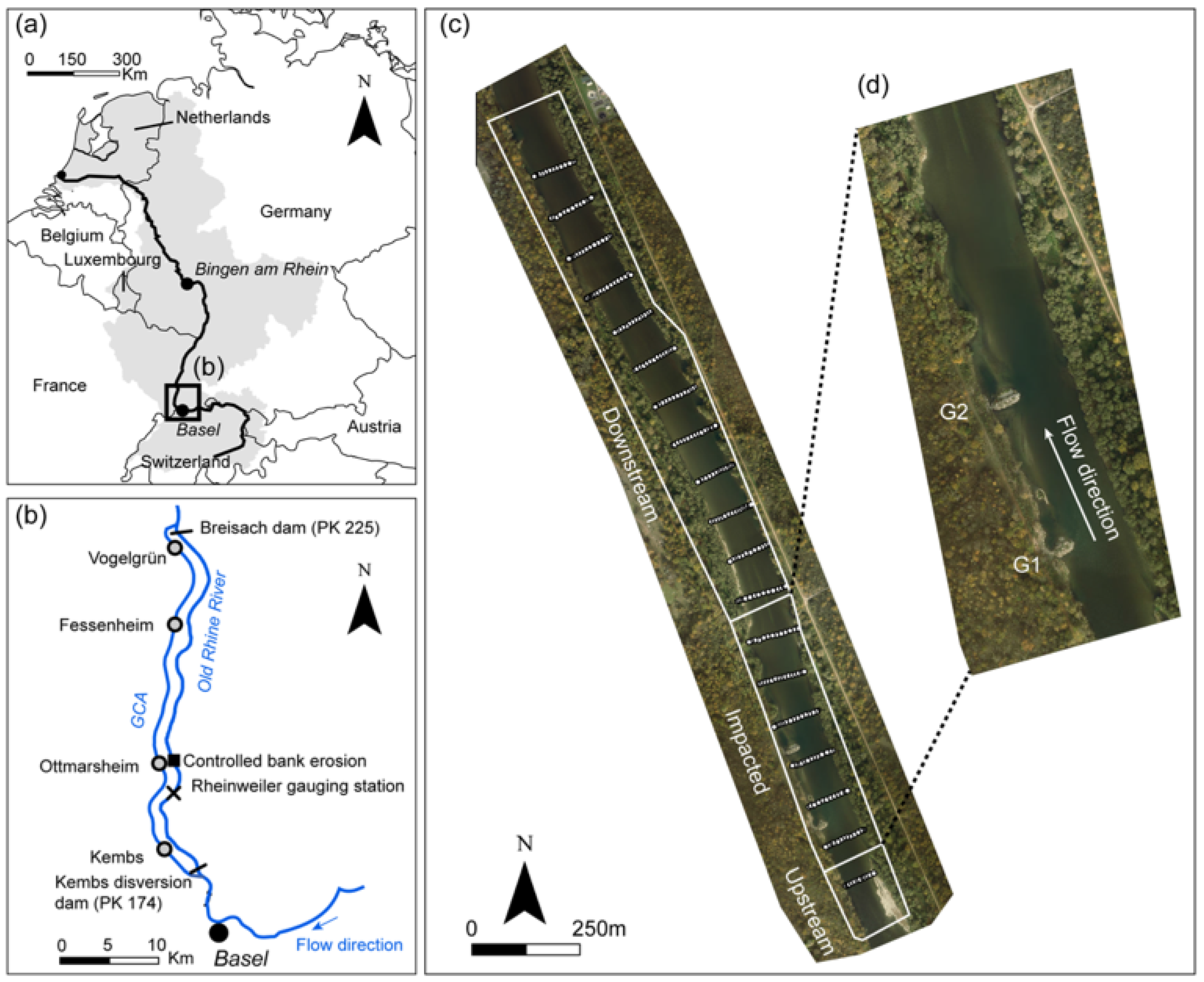
2.1. Study Area

The Rhine River is the third largest river in Europe with a length and drainage basin equal to 1250 km and 185,000 km 2 , respectively. The Upper Rhine, a 300 km long section located between Basel and Bingen-am-Rhein, shows a nivo-glacial hydrological regime (Figure 1a). The mean annual discharge has been estimated at 1059 m 3 /s at the Basel gauging station (during the period 1891–2008) [38]. Since the beginning of the 19th century, the Upper Rhine has been profoundly impacted by several engineering works. These works induced the severe degradation of both geomorphological conditions (e.g., simplification of channel patterns, narrowing and stabilization of the main channel, bed incision, and armoring) and ecological function (losses of habitat diversity and dynamics). These effects were notably observed along a 50 km by-passed reach parallel to the Grand Canal d’Alsace (GCA) downstream of Basel [39] (Figure 1b). Since 2010, several restoration actions, including an increase in instream flow [40], gravel augmentations [41,42], and controlled bank erosion with the implementation of two transverse groynes [43], have been performed along this by-passed reach to enhance the bedload transport and morphodynamics therein and thus diversify aquatic and riverine habitats. In December 2010, the instream flow entering the Old Rhine increased from a quasi-constant discharge of 20–30 m 3 /s to a seasonally varying discharge of 52–150 m 3 /s in accordance with the life cycle of native fish species [44]. An initial experiment of controlled bank erosion was implemented in 2013 over a span of 300 m on the upstream part of the Old Rhine (KP 191.30–191.60; April–May 2013). This ecological action consisted of removing the bank protection and three old groynes built during the beginning of the 20th century (Figure 1d) and implementing two new transverse groynes within the flow channel to maximize flow velocities and shear stresses along the bank. The location and shape of these groynes had been previously defined through numerical and physical modeling to promote bank erosion, deliver sediment into the channel, and avoid any damage to human construction due to uncontrolled lateral erosion [45].
The monitoring was composed of four states (S i ), namely, an initial state (S 0 ) and three periods (P i ). Since this restoration, the flood peaks reached 2600 m 3 /s, 1400 m 3 /s and 1590 m 3 /s during P 1 , P 2 and P 3 , respectively (Figure 2). The flood discharges were measured at the Rheinweiler gauging station (located 5 km upstream of the restored site). No tributaries are located between this gauging station and the studied reach. Following these flood events, only few bank erosion events occurred. However, significant and unexpected geomorphological changes, of the bathymetry and bed grain size, were observed that show that transverse groynes had significant effects on aquatic habitats. The latter motivated the implementation of our research strategy.

2.2. Data Collection and Processing

2.2.1. Field Monitoring

Field monitoring was performed following a before-after-control-impact (BACI) framework [35] on three river sections: the upstream, impacted, and downstream sections (Figure 1). The upstream and downstream sections were used as control sections, and the impacted section was judged according to the impact of the restoration action.
In March 2013 (S 0 ), a bathymetric survey was performed using a Tritech PA500 single beam echo-sounder (Tritech International Limited, Aberdeenshire, Scotland) to survey the channel bathymetry. Since March 2014 (S 1 ), yearly airborne topo-bathymetric LiDAR surveys have been performed to systematically characterize the channel geometry with a high resolution in both above-water and underwater conditions along the first upstream 20 km of the by-passed channel. For S 1 , a Riegl VQ-820-G (RIEGL Laser Measurement Systems, Horn, Austria) sensor was used, whereas an Optech Titan sensor (Teledyne Optech, Vaughan Canada) was used during S 2 (March 2016) and S 3 (March 2017) (Figure 3). High-resolution digital elevation models (DEMs; cell size of 0.25 m 2 ) were produced using Arcmap software v.10.3 (ESRI, Redlands, California, USA). The channel elevation changes for each period (P i ) were calculated by the DEMs of difference (DoDs) between two surveys. Field measurements of water depths and flow velocities and visual estimates of the bed grain size were conducted along cross-sections (n = 18) at a spacing of 100 m with 12 to 19 sampling points for each cross-section, and the measurements were collected by a private company [47,48,49,50]. All sampling points were georeferenced by a global positioning system (Promark 700). The same sampling points were recorded during each survey to evaluate the changes in physical parameters as accurately as possible (Figure 1c). A rod and a Nautilus C2000 current meter were used to measure the water depth and the flow velocity, respectively, at 0.4 times the water depth from the channel bottom using a boat. A bathyscope was used to qualitatively estimate the bed grain size according to the ordinal classification of [51]. The discharges during data collection for S 1 , S 2 , S 3 , and S 4 were approximately 67 m 3 /s, 52 m 3 /s, 70 m 3 /s, and 70 m 3 /s, respectively (Figure 2).

2.2.2. Grain Size Quantification

The qualitative estimates of the bed grain size were transformed into quantitative values on the basis of the EVHA codification [52]:
Grain size value = 0.2 * coarsest substrate + 0.4 * dominant substrate 1 + 0.4 * dominante substrate 2
In the case of only one dominant substrate:
Grain size value = 0.2 * coarsest substrate + 0.8 * dominant substrate
The bed grain size along the entire study reach was interpolated following the triangulation interpolation method.

2.2.3. Hydraulic Models

A two-dimensional hydraulic model was performed for each state (S i ) by using HEC-RAS software (v.5.0.3). The topo-bathymetric data for the models were provided by high-resolution DEMs. Each model run was calibrated with the field measurements of the water depths and flow velocities performed at each S i and correlated with the daily discharges provided by the Rheinweiler gauging station (Figure 1b and Figure 2). Sensitivity analyses of the Manning coefficient were performed to determine the best calibration values for modeling purposes. The values of the Manning coefficient varied over the four S i from 0.025 to 0.030, similar to the values proposed by Chow [53] and Benson et al. [54] for rivers similar to this by-passed reach. For each state, the water depths and flow velocities were modeled for the studied reach at 52 m 3 /s because this discharge has been the most frequent daily discharge recorded since December 2010.

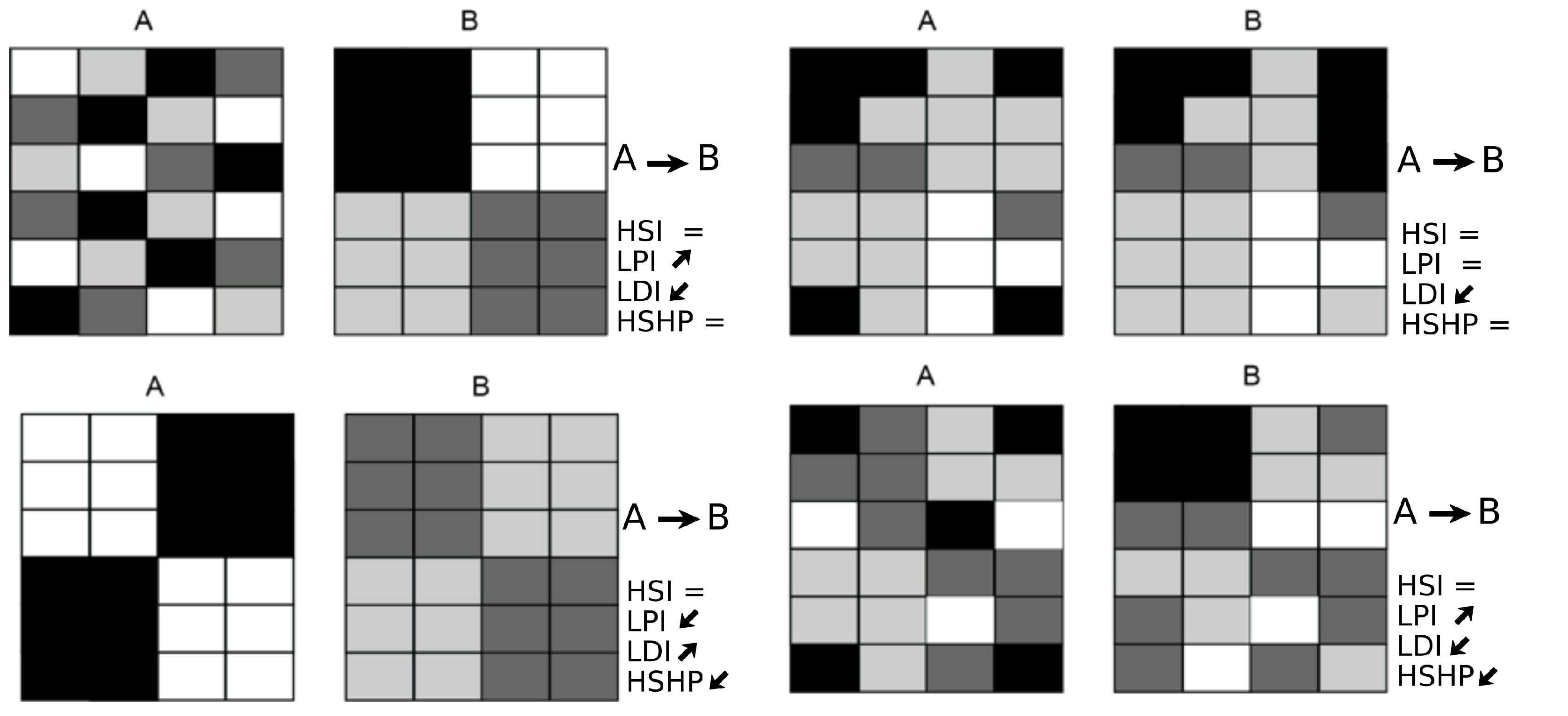
2.2.4. Estimation of Aquatic Habitat Heterogeneity

Habitat heterogeneity was estimated using the eco-hydro-morphological index of diversity (EHMID) developed by [55] following the hydro-morphological index of diversity (HMID) proposed by [56]. The EHMID was slightly modified because the suitability curves following the grain size were based on the EVHA codification rather than the median grain size, as proposed by [55]. The metric was normalized by the section width, the resulting metric, nEHMID m , was calculated as follows:
n E H M I D m = ( 1 + ( θ v μ v ) ) 2 ( 1 + ( θ d μ d ) ) 2 ( 1 + ( θ g μ g ) ) 2
where ( 1 + ( θ v μ v ) ) 2 , ( 1 + ( θ d μ d ) ) 2 and ( 1 + ( θ g μ g ) ) 2 correspond to the partial diversity of the flow velocities (m.s 1 ), water depths (m), and bed grain sizes (codification), respectively.
The cross-section diversity (CSD) developed by Gostner et al. [56] was calculated for each cross-section to evaluate the relation between the physical parameters changes and the channel geometry changes. This metric was calculated with the following formula:
C S D = i = 1 n | Δ Y i | i = 1 n 1 X i
with
| Δ Y i | = Y i 1 Y i
where | Δ Y i | is the absolute height difference in the channel bottom between two consecutive points on a cross-section (m) and X i is the distance between those two points (m).

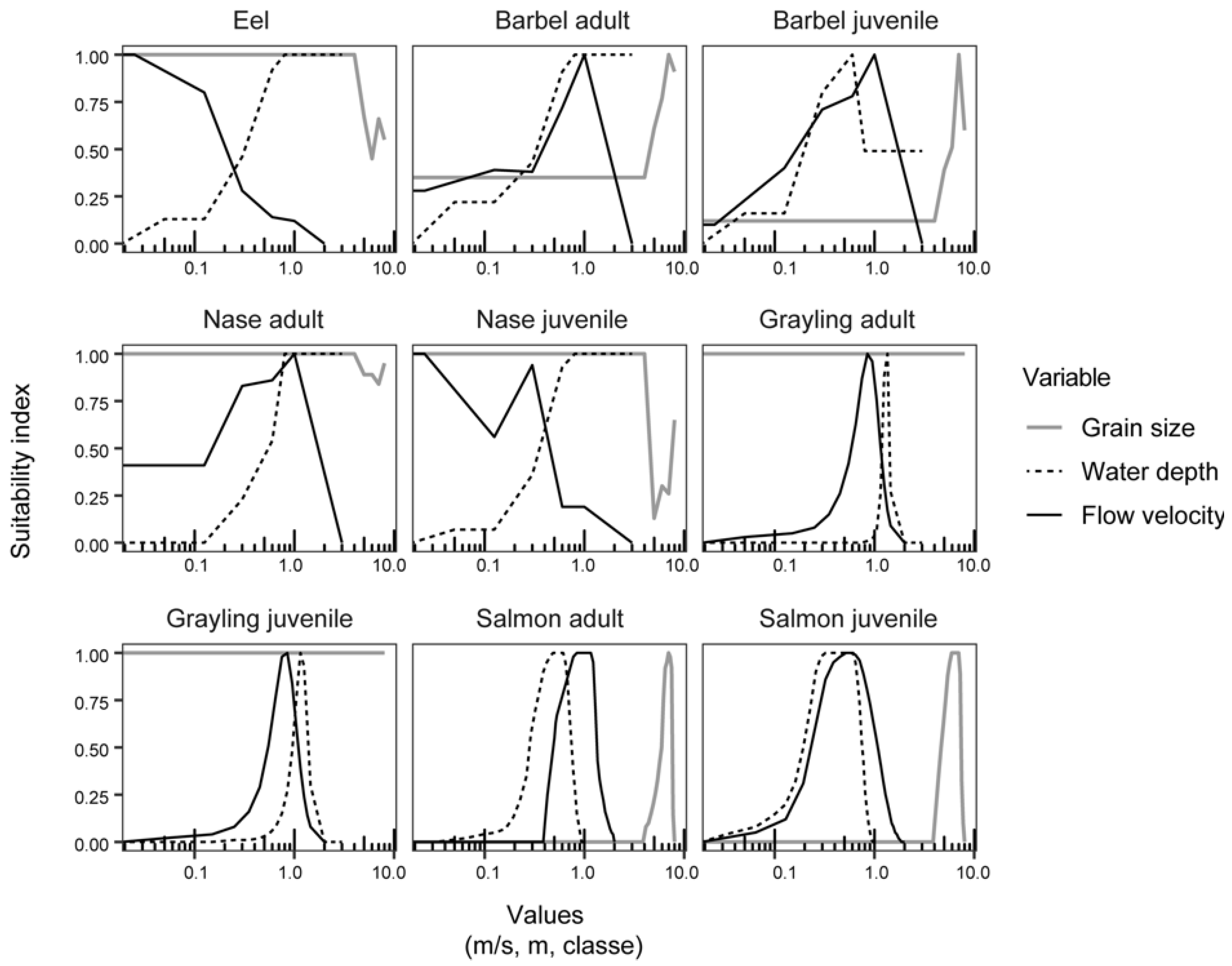
2.2.5. Fish Habitat Models and Metrics

In this study, the suitability curves were based on statistical relationships defined for six large rivers in France according to field observations (Table 1). Suitability curves were established for three categories of physical parameters: water depth, flow velocity, and bed grain size (Figure 4). We estimated the habitat quality for five native fish observed in the study reach (mostly for the adult and juvenile life stages): barbel (Barbus barbus), nase (Chondrostoma nasus), grayling (Thymallus thymallus), salmon (Salmo salar), and eel (Anguilla anguilla).
Habitat suitability was estimated according to the suitability index (SI) calculated at the cell scale (0.25 m 2 for each physical variable varying from 0 (bad habitat quality) to 1 (excellent habitat quality) (Figure 3). According to [29,57,58], the combined suitability index (CSI), which corresponds to the product among the SI values of the n physical variables was calculated as follows:
C S I i = ( S I i j ) 1 / n
where i, j, and n correspond to the cell in which the computation is occurring, the physical parameter being multiplied, and the number of physical parameters, respectively.
From the CSI, the habitat suitability index (HSI) was calculated to estimate the habitat suitability at the section scale and calculated it as follows [29,59,60]:
H S I = 1 A i = 1 n a i C S I i
where a i is the surface area of cell i and A is the cross-sectional area of the section being studied (upstream, impacted, and downstream sections). All indices were calculated by using ArcGIS v10.3 software based on Python scripts and calculated from the results of the two-dimensional hydraulic model runs. In addition, the following three metrics were calculated using FRAGSTATS software v.4.0 to take into account both the configuration and the composition of the riverscape (Figure 4):
i
The highly suitable habitat proportion (HSHP):
H S H P = a i j 2 A
ii
The largest patch index (LPI):
L P I = m a x a i j A
iii
The landscape division index (LDI):
L D I = 1 i = 1 m i = j n a i j A
where a i j is equal to the surface area of patch ij and A is the cross-sectional area of the section being studied. These three metrics were calculated for the highly suitable habitat, which corresponds to a CSI equal to or greater than 0.5. All of the metrics were estimated for the upstream, impacted, and downstream sections and for each S i (Figure 1c and Figure 3).
Furthermore, a synthetic index varying from 0 (bad) to 1 (excellent) was developed to quantify habitat suitability; this index is called the synthetic habitat suitability index (SHSI), which combines the four previous metrics with identical weighting, and is calculated as follows:
S H S I = H S I + H S H P + L P I + ( 1 L D I ) 4
Then, we calculated the temporal change ratio (TCR) of the SHSI for each period as follows:
T C R ( % ) = S H S I S i + 1 S H S I S 0 100

3. Results

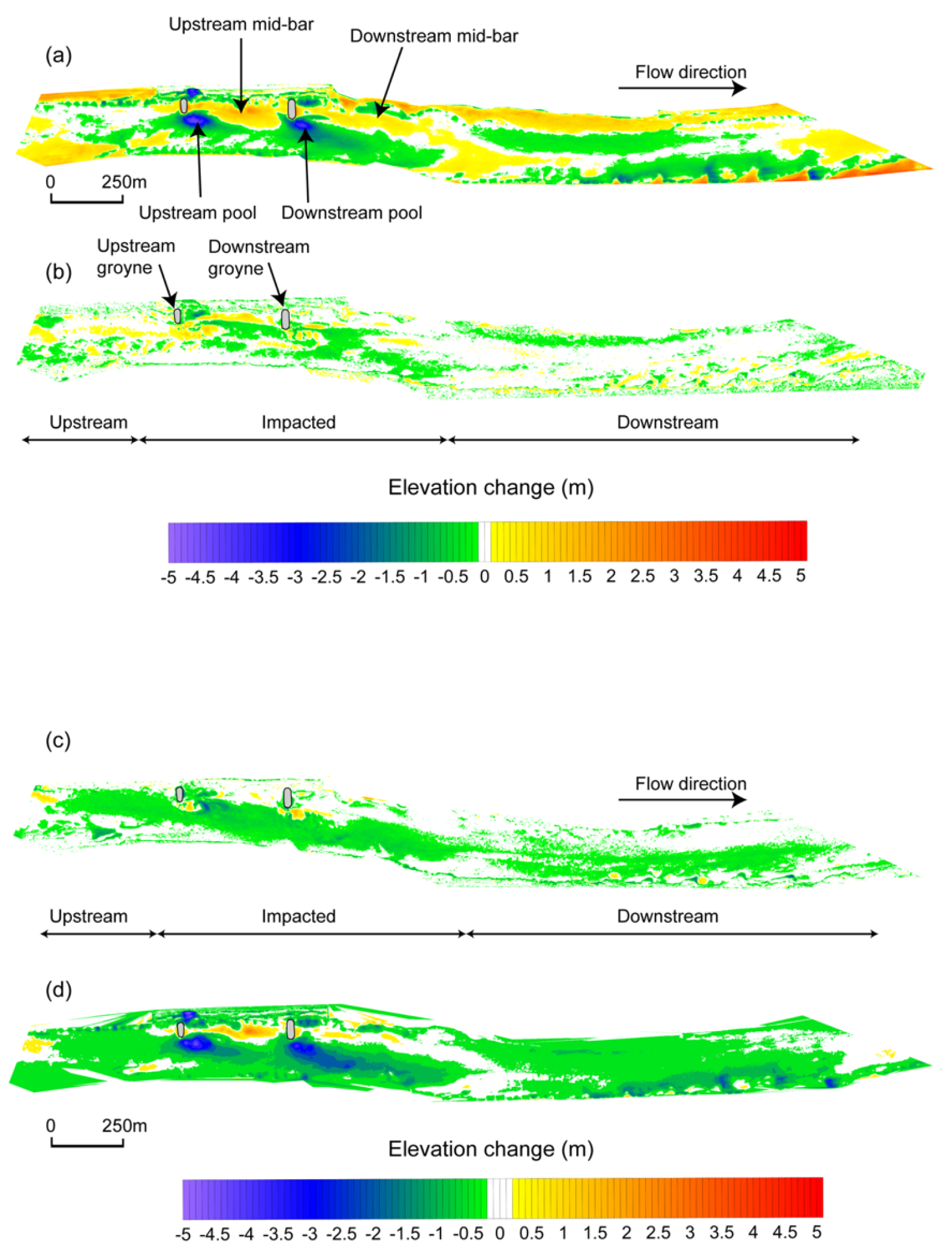
3.1. Channel Responses

During P 1 , contrasting channel adjustments occurred following the intense flood of May–June 2013 (Q i x < 15 years). The bed was scoured by 0.1 m to 0.5 m in the upstream section, whereas both bed scouring (max. of 1 m) and bed deposition (max. of 0.7 m) occurred on the two riffles located in the downstream section (Figure 5a). In the impacted section, new macroforms appeared with the formation of two mid-bars downstream of the two artificial groynes, where the deposition thickness ranged from 0.1 m to 2.5 m (Figure 5a–c), and scouring (max. of 4 m) occurred in two pools at the eastern extremity of the artificial groynes. During P 2 , the upstream and downstream sections morphologically evolved less than during P 1 , with less than 0.5 m of scouring and deposition occurring. Moreover, in the impacted section, the bed was globally eroded. During P 3 , generalized scour of the bed occurred along the whole study reach, reaching a maximum of 2 m locally in the upstream pool. Nevertheless, macroforms were clearly still present during the whole monitoring period (Figure 5d). These channel responses induced a significant increase in the CSD values within the impacted section during the whole monitoring period, whereas the CSD values in the upstream and downstream sections remained globally stable (Figure 6e).

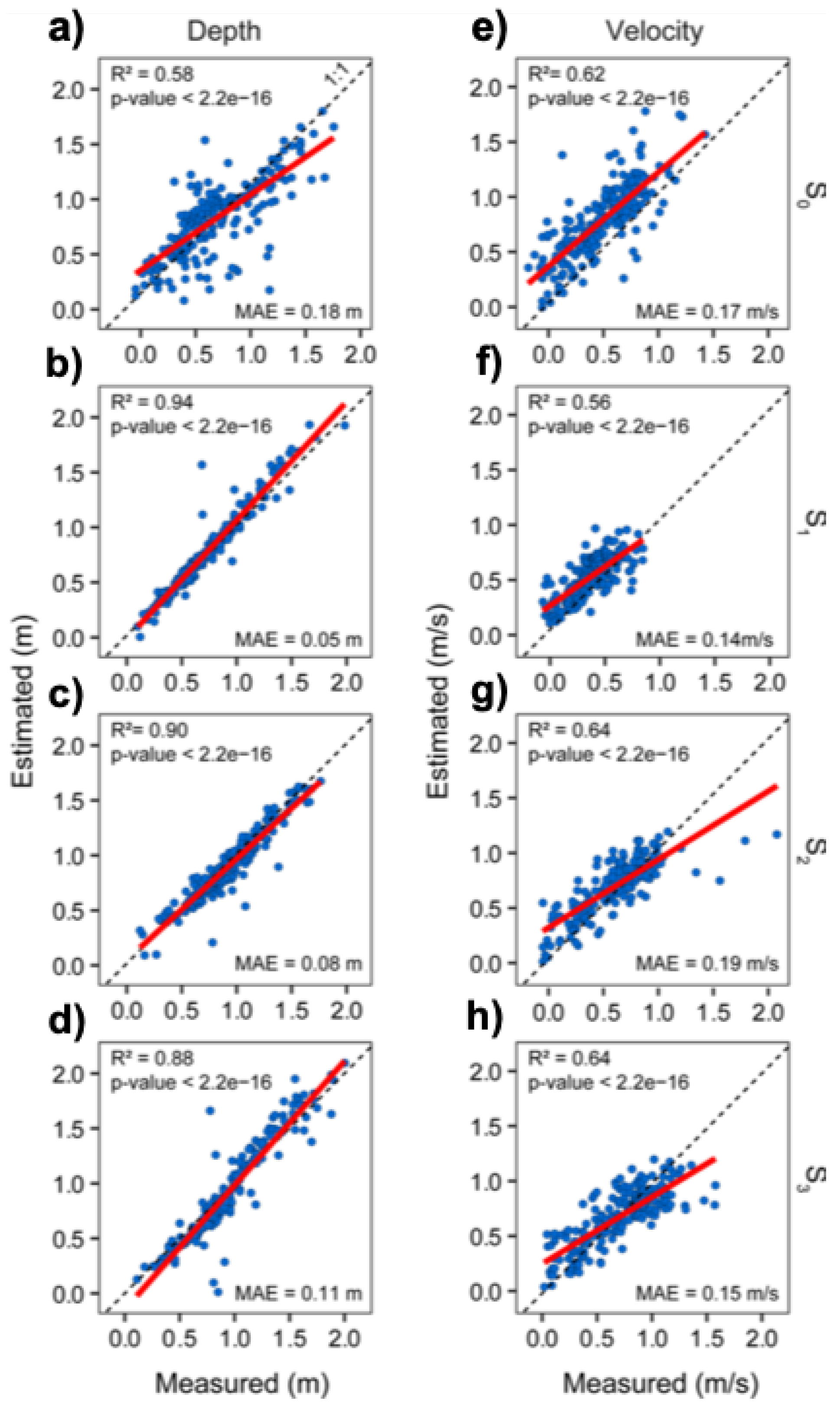
3.2. Precision of the Hydraulic Models

The hydraulic models reliably simulated the two hydraulic variables, namely, the water depth and flow velocity. The mean absolute error (MAE) values for the simulated water depths are equal to 0.18 m, 0.05 m, 0.08 m, and 0.11 m for S 0 , S 1 , S 2 , and S 3 , respectively (Figure 6a–d). Likewise, the MAE values for the simulated flow velocities are equal to 0.17 m/s, 0.14 m/s, 0.19 m/s, and 0.15 m/s for S 0 , S 1 , S 2 , and S 3 , respectively (Figure 6e–h). The lower accuracy of the simulations related to the first survey during S 0 , especially for the water depths, is probably due to the lower quality of the DEM [29], which was produced using a single-beam echosounder rather than airborne LiDAR topo-bathymetric surveying, which is characterized by a high density of points per square metre.

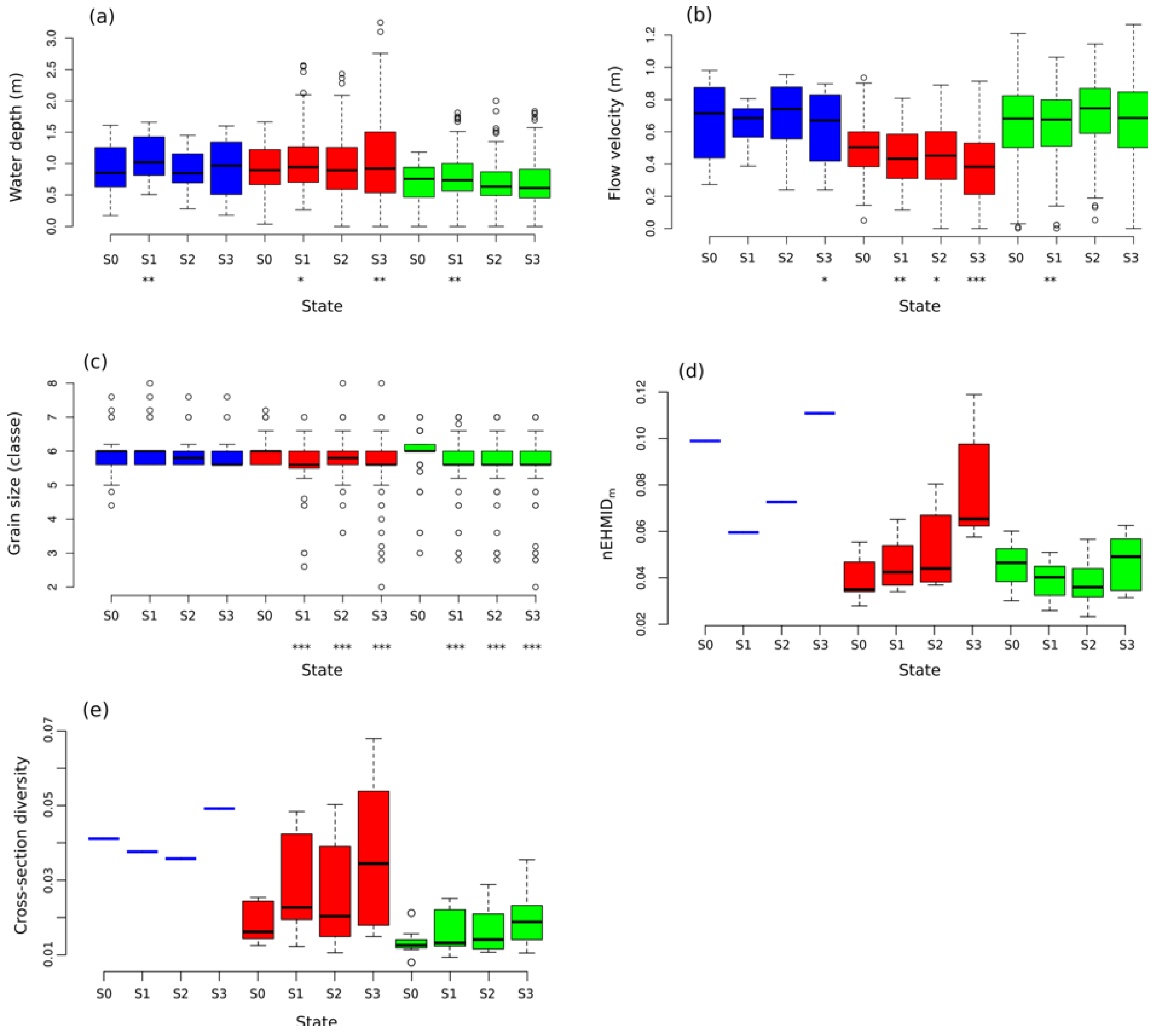
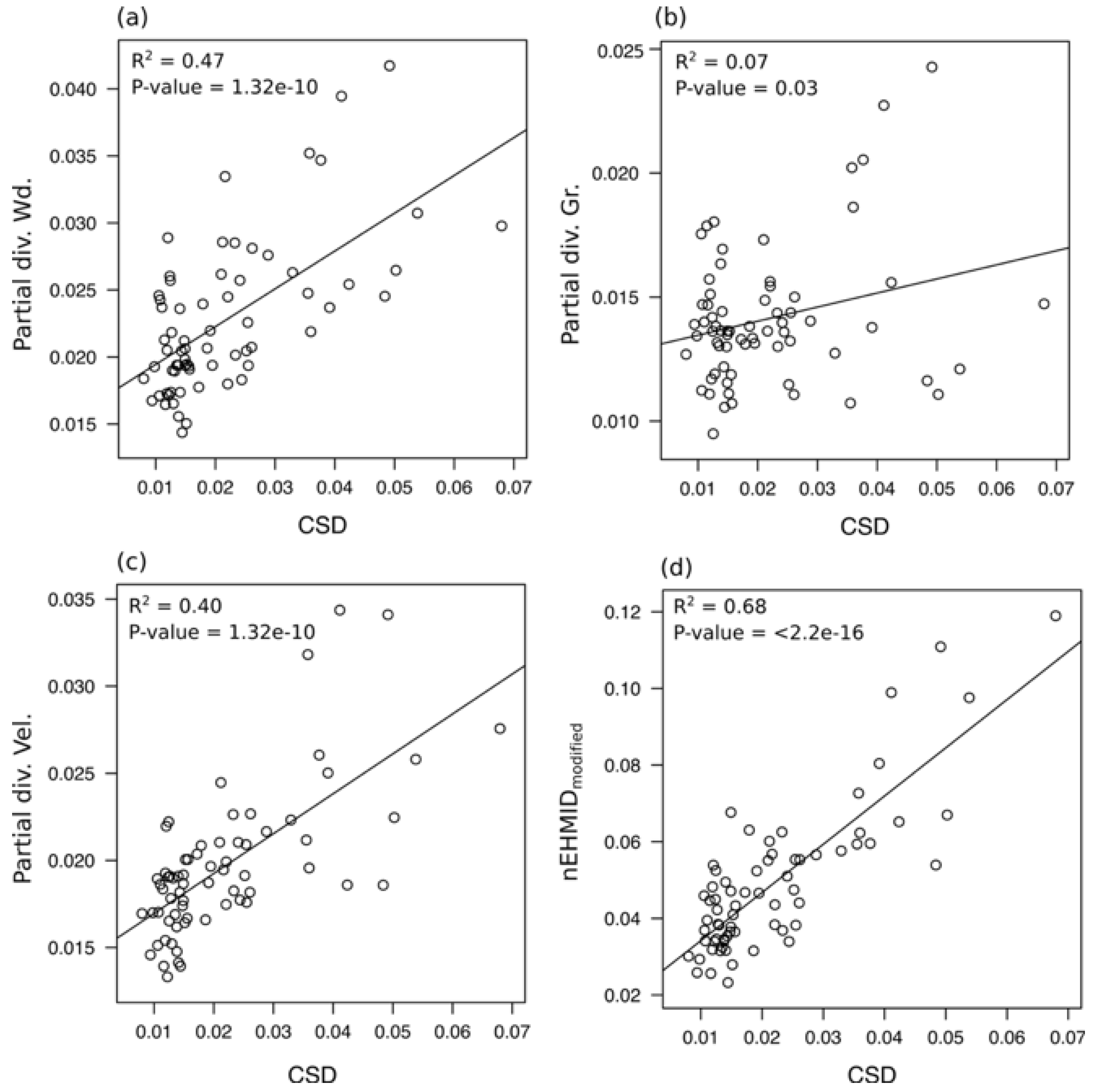
3.3. Temporal Evolution of Habitat Heterogeneity

During the whole monitoring period, significant changes were observed throughout the upstream section with an increase in the water depth at S 1 and a reduction in the flow velocity at S 3 . Within the downstream section, significant fining of the bed grain size was observed over the whole monitoring period, and slightly significant changes in the water depth and flow velocity were observed at S 1 (Figure 7a–c). In the impacted section, significant changes in all three physical parameters were observed over the whole monitoring period with decreases in the flow velocity and bed grain size and an increase in the water depth (Figure 7a–c).
Changes in the physical parameters along the impacted section induced progressive increases in the CSD and nEHMID m values. The mean CSD was equal to 0.034, 0.037, 0.043, and 0.060 for S 0 , S 1 , S 2 , and S 3 , respectively, and the mean nEHMID m was equal to 0.039, 0.046, 0.051, and 0.078 for S 0 , S 1 , S 2 , and S 3 , respectively. Relatively small changes occurred in both the CSD and the nEHMID m values along the downstream section with mean CSD values equal to 0.038, 0.032, 0.031, and 0.039 for S 0 , S 1 , S 2 , and S 3 , respectively, and mean nEHMID m values equal to 0.045, 0.039, 0,038, and 0.047 for S 0 , S 1 , S 2 , and S 3 , respectively. The upstream section showed a singular pattern comprising a decrease followed by an increase (Figure 7e). Statistically significant linear relationships were found (at a 95% confidence interval) between the partial diversity of the water depth and flow velocity and the CSD index, whereas lower significance was found for the partial diversity of the grain size (Figure 8a–c). The relationship between the nEHMID m and CSD was almost stronger than these relationships (Figure 8d).

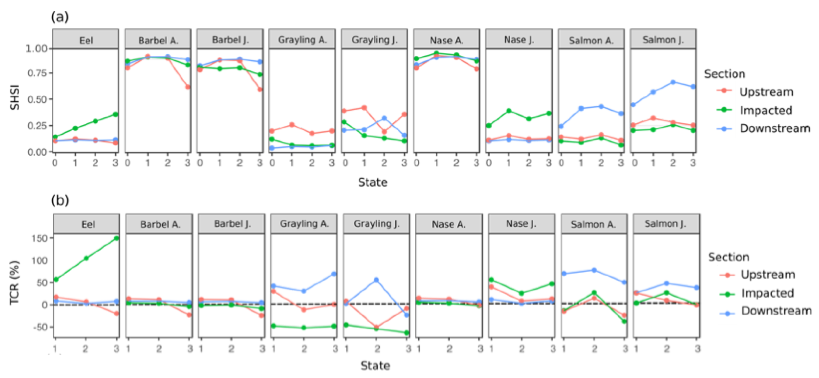
3.4. Temporal Evolution of Fish Habitat Suitability

For the whole monitoring period and throughout the whole study reach, the highest values of the SHSI (>0.50) were observed for barbel at both the adult and the juvenile life stages and for nase at the adult life stage (Figure 9a). In contrast, the lowest values of the SHSI (<0.45) were observed for all other species on the three sections, except for salmon at the juvenile stage in the downstream section, for which the SHSI ranged from 0.45 to 0.66.
Significant changes in the TCR values were calculated for both the impacted and the downstream sections (Figure 9b). In the impacted section, the TCR values were positive for both eel and juvenile nase species with a maximum at S 3 equal to +149% and juvenile nase with a maximum at S 1 equal to +57%. At S 2 , positive TCR values in the downstream section were related to juvenile and adult salmon species with maxima equal to +78% and +48%, respectively, and adult grayling with a maximum of +57% at S 3 (Figure 9b). Globally, during the monitoring period, the TCR values calculated within the upstream section were stable, except for juvenile grayling during S 2 with a TCR value equal to −52% (Figure 9b).

4. Discussion

4.1. Channel Responses and Habitat Heterogeneity

The results show that the implementation of the two groynes induced significant channel responses. Two mid-bars were created downstream of the two groynes due to the reduction in the flow velocities and the formation of countercurrents downstream of the groynes. Sediments were generated by the scour of the two pools and by bank erosion, both following the reduction in the area of the wetted section induced by the two groynes, while other sediments were produced from residual bedload transport within the main channel upstream of the restoration site [39]. These channel responses are in accordance with previous modeling and field reports [45,61,62]. Field monitoring showed that the flow velocities were reduced along the impacted section during the whole monitoring period (four years) while maintaining the same range of flow velocities as measured during the pre-restoration period for both the upstream and the downstream sections (Figure 7b). Concerning the bed grain size, we observed significant fining of the bed grain size in both the impacted and the downstream sections. Finer grain sizes may be related to the deposition of fine sediments provided by bank erosion [43] and/or by the scouring of the two pools (Figure 7c). These finer particles may also originate from the upstream reaches due both to probable local bank erosion and to break-up of the pre-existing bed armor layer following the intense flood of May–June 2013 (Q 15 ) [42]. Indeed, the break-up of this armor layer induces the entrainment of the subsurface layer, which contains particles that are finer than those within the surface armor layer [63]. Along the regulated lower Ebro River, the authors in [64] showed that the bed armor layer was broken up during intensive flood events and was subsequently re-established during lower flood events. The authors in [65] and [39] further demonstrated that residual geomorphological processes occurred along this by-passed section during intensive flood events, as shown by bed elevation changes.
This study indicates that the transverse groynes significantly increased the physical habitat heterogeneity, whereas few changes occurred in the upstream and downstream sections (Figure 5 and Figure 7). The empirical relationship found between the nEHMID m and CSD indicates that habitat heterogeneity increases as the channel cross-section becomes more diversified (Figure 8d). This finding validates the first hypothesis that the implementation of transverse groynes would enhance habitat heterogeneity in the impacted section. The increase in the nEHMID m values along the impacted section suggests that the geomorphological effects of this restoration are still effective after several floods and may persist as long as the two groynes remain, probably over several decades (Figure 5d).
In such large and heavily impacted by-passed systems within which habitat improvement is critical, such experiences question the opportunity of introducing new groynes in specific reaches to enhance habitat suitability. Such active restoration measures have shown positive effects on fish responses [17,18]. These results raise questions regarding environmental ethics related to the increased use of artificial features to enhance ecological conditions. To restore geomorphic processes in a more sustainable way and achieve improvements to aquatic and riverine habitats efficiently, the authors in [39,42,66] recommended combining gravel augmentations and channel widening. More specifically, channel widening should be performed downstream of gravel augmentations, promoting the deposition of some injected sediments and potentially diversifying aquatic and riverine habitats [41,67]. Several methods may be tested to perform channel widening, such as the removal of bank protection, the partial removal of historical groyne fields and/or the excavation of floodplain areas connected to the channel. In the last option, excavated sediments should be stored temporarily on an island and injected upstream periodically depending on the hydrological regime. However, such operations, which must avoid any risks to human activities (e.g., navigation and flood control), depend strongly on the financial resources available and local technical characteristics. Furthermore, some small interventions may also be tested to enhance local fish habitats [14,16] to reconfigure existing historical groynes and/or introduce wood structures [68].

4.2. Temporal Evolution of Fish Habitat Suitability

From four landscape metrics, a synthetic metric, namely, the SHSI, was developed to estimate the quality of fish habitat suitability by integrating changes in the riverscape in terms of both the composition and the configuration, which are rarely studied. It is essential to estimate these factors, notably in the context of river restoration, to integrate all possible riverscape changes because ecological processes at the population and community levels are highly affected by the composition and configuration of a riverscape [32]. Our results highlight that the SHSI metric can be adopt to evaluate habitat changes because it integrates physical variables that are key indicators of habitat diversity (Figure 7e and Figure 9a).
This study demonstrates that the habitat suitability of the studied reach was higher for a larger fish species than before the restoration work. Indeed, an improvement for species that like low flow velocities and low bed grain size conditions occured during the monitoring period on the impacted section (Figure 3 and Figure 9). These results are explained by the reduction in flow velocities induced by the two artificial groynes (Figure 7b) and the deposition of fine sediments downstream of those groynes [69]. Taking into account the whole study reach, the restoration clearly increased the habitat suitability for a larger number of native fish species than in the pre-restoration conditions (Figure 9).
Indeed, the results of electric fishing conducted along the impacted section showed that the fish communities captured were composed mostly of rheophilic species [43], and eel individuals were present along the impacted section for the first time after the first post-restoration flood of May–June 2013. Interestingly, the results of field fish surveys are in accordance with the results obtained from fish habitat models. Furthermore, these results should be consolidated by further field surveys of fish communities.
An unexpected result was the improvement in the fish habitat suitability for salmon in the downstream section due to sustainable fining of the bed grain size over the four years (Figure 7c and Figure 9a,b). This finding highlights that the bed grain size is as important as the hydraulic conditions for improving the habitat suitability of targeted species. Therefore, in some cases, heavy restorations could be avoided by focusing on the bed grain size rather than only on the hydraulic conditions. Chardon et al. (submitted) [70] showed the ability of gravel augmentations to restore potential spawning areas for rheophilic species due to the preferential deposition of the injected sediments on riffles. This finding also shows that it is important to consider grain size issues in habitat suitability approaches because the bed grain size is a critical ecological parameter that notably concerns lithophilous species and can be improved by specific restoration measures, such as providing a coarse sediment supply from artificial gravel augmentations or bank erosion [26,71].

4.3. Eco-Hydraulic Modelling, a Tool for River Restoration Design

Currently, a large amount of financial resources is dedicated to river restoration. The authors in [10] estimated that the restoration of 1 ha of a European river costs, on average, 310,000 €. Furthermore, despite the high costs of restoration actions, several authors highlighted that restoration projects have no clear goals and suffer from a lack of planning [72]. With the introduction of or recent developments in remote sensing methods such as airborne topo-bathymetric LiDAR and hydraulic open-source software, it is now possible to establish two-dimensional hydraulic models and characterize fluvial habitats at finer scales along larger reaches than was previously possible. Hydro-ecological models are a powerful tool for restoration planning to (i) evaluate the degradation states of river channels, (ii) test several restoration designs, and (iii) define the best among those designs according to restoration objectives [73].
Nevertheless, these models have some shortcomings. Most studies of fish habitat modeling focus on hydraulic parameters because the flow conditions are generally considered the most important factors that influence the distributions of fish populations and control, at least partly, some other environmental parameters (e.g., water temperature, water oxygenation, and pollutant concentrations) [74,75]. However, these parameters may limit other factors because the influences of physical parameters decrease in the downstream direction [76], and their influences may increase in the future in the context of global change and increasing land use pressure. Although fish species are able to adapt to climate change by modifying their phenology, physiology, and distribution [77,78], a delay can be observed [79]. Moreover, several species may not be able to adapt to environmental changes [78], which could lead to declines in population and profound community modifications. In the same way, water physico-chemistry and some biotic factors (e.g., food availability, competition, predation, parasitism, and invasion) may also be significant drivers of the fish population distribution and abundance [80,81,82]. Supplementary research must be conducted to better understand the impacts of abiotic, biotic, and chemical factors and their inter-relations with the repartition and abundance of fish populations to sustain them in a changing world.

5. Conclusions

This paper highlights the advantages of using a riverscape approach rather than a classic approach in fish-habitat modeling. This riverscape approach allowed us to evaluate landscape dynamics in terms of the changes in their configuration and composition, which are crucial in the context of river restoration. The restoration work induced a rise in habitat suitability for a large number of native fish species compared with the pre-restoration conditions. In addition, this study reveals that the improvement of grain size conditions can be as efficient as improvements to flow conditions at enhancing the habitat suitability for some targeted fish species, notably for salmon species. Finally, the implementation of groynes could be a strategy for improving fish habitats, but only where more functional and natural restoration options are impossible.

Author Contributions

Investigation, V.C.; Methodology, V.C.; Resources, A.B. and A.C.; Supervision, L.S. and H.P.; Writing—original draft, V.C.; Writing—review and editing, L.S., H.P., J.-N.B. and C.S. All authors have read and agreed to the published version of the manuscript.

Funding

This research was funded by the company Electricité de France (EDF) within the research collaboration “Redynamization of the Old Rhine—years 2014–2018” (EDF 5910132058).

Acknowledgments

The authors thank their colleagues who provided fieldwork assistance: Jérôme Houssier, Jordane Serouilou, Grzegorz Skupinski, David Eschbach and Francis Bruckmann. The authors also thank ECOTEC, which provided the flow velocity, water depth, and grain size field measurements, and Rennes University for the airborne LiDAR topo-bathymetric surveys. The authors also want to thank three anonymous reviewers who greatly contributed to improving to this paper by providing helpful reviews of an earlier version of this manuscript. This work was performed within the framework of the EUR H2O’Lyon (ANR-17-EURE-0018) of the University of Lyon within the program “Investissements d’Avenir” operated by the French National Research Agency (ANR).

Conflicts of Interest

The authors declare no conflict of interest.

Abbreviations

The following abbreviations are used in this manuscript:
CSDcross-section diversity
GCAgrand canal d’alsace
HSHPhighly suitable habitat proportion
HSIhabitat suitability index
LPIlarge patch index
nEHMIDmnormalized eco-hydro-morphological index of diversity modified
SHSIsynthetic habitat suitability index
TCRtemporal change ratio
WUAweighted usable area

References

  1. Alexander, J.; Wilson, R.; Green, W. A Brief History and Summary of the Effects of River Engineering and Dams on the Mississippi River System and Delta; Circular 1; U.S. Geological Survey Circular 1375: Reston, VA, USA, 2012; p. 43.
  2. Grill, G.; Lehner, B.; Thieme, M.; Geenen, B.; Tickner, D.; Antonelli, F.; Babu, S.; Borrelli, P.; Cheng, L.; Crochetiere, H.; et al. Mapping the world’s free-flowing rivers. Nature 2019, 569, 215–221. [Google Scholar] [CrossRef] [PubMed]
  3. Cooper, A.R.; Infante, D.M.; Daniel, W.M.; Wehrly, K.E.; Wang, L.; Brenden, T.O. Assessment of dam effects on streams and fish assemblages of the conterminous USA. Sci. Total Environ. 2017, 586, 879–889. [Google Scholar] [CrossRef] [PubMed]
  4. Jellyman, P.G.; Harding, J.S. The role of dams in altering freshwater fish communities in New Zealand. N. Z. Mar. Freshw. Res. 2012, 46, 475–489. [Google Scholar] [CrossRef] [Green Version]
  5. Morandi, B.; Piégay, H.; Lamouroux, N.; Vaudor, L. How is success or failure in river restoration projects evaluated ? Feedback from French restoration projects. J. Environ. Manag. 2014, 137, 178–188. [Google Scholar] [CrossRef] [PubMed]
  6. Bernhardt, E.S.; Palmer, M.A. Restoring streams in an urbanizing world. Freashw. Biol. 2007, 52, 738–751. [Google Scholar] [CrossRef]
  7. Henry, C.P.; Amoros, C.; Roset, N. Restoration ecology of riverine wetlands: A 5-year post-operation survey on the Rhône River, France. Ecol. Eng. 2002, 18, 543–554. [Google Scholar] [CrossRef]
  8. Palmer, M.A.; Bernhardt, E.S.; Allan, J.D.; Alexander, G.; Shah, J.F.; Galat, D.L.; Hart, D.D.; Jenkinson, R.; Lave, R.; Sudduth, E. Standards for ecologically successful river restoration. J. Appl. Ecol. 2005, 42, 208–217. [Google Scholar] [CrossRef]
  9. Palmer, M.A.; Holly, L.M.; Bernhardt, E. River restoration, habitat heterogeneity and biodiversity: A failure of theory or practice? Freshw. Biol. 2010, 55, 205–222. [Google Scholar] [CrossRef]
  10. Szalkiewicz, E.; Jusik, S.; Grygoruk, M. Status of and perspectives on river restoration in Europe: 310,000 Euros per hectare of restored river. Sustainabilty 2018, 10, 129. [Google Scholar] [CrossRef] [Green Version]
  11. Schmutz, S.; Hein, T.; Sendzimir, J. Landmarks, Advances, and Future Challenges in Riverine Ecosystem Management; Aquatic Ecology Series; Springer: Berlin, Germany, 2018; Volume 8, pp. 563–571. [Google Scholar]
  12. Kondolf, G.M.; Anderson, S.; Lave, R.; Pagano, L.; Merenlender, A.; Bernhardt, E.S. Two Decades of River Restoration in California: What Can We Learn? Restor. Ecol. 2007, 15, 516–523. [Google Scholar] [CrossRef]
  13. Tonra, C.M.; Sager-Fradkin, K.; Morley, S.A.; Duda, J.J.; Marra, P.P. The rapid return of marine-derived nutrients to a freshwater food web following dam removal. Biol. Conserv. 2015, 192, 130–134. [Google Scholar] [CrossRef]
  14. Ramler, D.; Keckeis, H. Effects of large-river restoration measures on ecological fish guilds and focal species of conservation in a large European river (Danube, Austria). Sci. Total Environ. 2019, 686, 1076–1089. [Google Scholar] [CrossRef] [PubMed]
  15. Yossef, M.F.M. Literature Review: The Effect of Groynes on Rivers; Delft University of Technology Faculty of Civil Engineering and Geosciences Section of Hydraulic Engineering: Delft, The Netherlands, 2002; p. 58. [Google Scholar]
  16. Collas, F.P.; Buijse, A.D.; van den Heuvel, L.; van Kessel, N.; Schoor, M.M.; Eerden, H.; Leuven, R.S. Longitudinal training dams mitigate effects of shipping on environmental conditions and fish density in the littoral zones of the river Rhine. Sci. Total Environ. 2018, 619–620, 1183–1193. [Google Scholar] [CrossRef] [PubMed]
  17. Shields, F.D.; Knight, S.S.; Cooper, M. Incised stream physical habitat restoation with stone weirs. Regul. Rivers Res. Manag. 1995, 10, 181–198. [Google Scholar] [CrossRef]
  18. Lacey, R.W.; Millar, R.G. Reach scale hydraulic assessment of instream salmonid habitat restoration. J. Am. Water Resour. Assoc. 2004, 40, 1631–1644. [Google Scholar] [CrossRef]
  19. Roberge, J.M.; Angelstam, P.E.R. Usefulness of the umbrella species concept as a conservation tool. Conserv. Biol. 2004, 18, 76–85. [Google Scholar] [CrossRef]
  20. Bain, M.B.; Jia, H. A habitat model for fish communities in large streams and small rivers. Int. J. Ecol. 2012, 2012, 8. [Google Scholar] [CrossRef] [Green Version]
  21. Moore, J. Fish Communities as Indicators of Environmental Quality in the West River Watershed. In Restoration of an Urban Salt Marsh An Interdisciplinary Approach; Yale University RIS Publishing: New Haven, CT, USA, 1997; pp. 178–196. [Google Scholar]
  22. Brazil, S.E.; Rodrigues, M.; Mattos, T.M.; Fernandes, V.H.; Martínez-capel, F.; Muñoz-Mas, R.; Araújo, F.G. Application of the physical habitat simulation for fish species to assess environmental flows in an Atlantic Forest Stream in South-eastern Brazil. Neotrop. Ichthyol. 2015, 13, 685–698. [Google Scholar] [CrossRef] [Green Version]
  23. Lamouroux, N.; Gore, J.A.; Lepori, F.; Statzner, B. The ecological restoration of large rivers needs science-based, predictive tools meeting public expectations: An overview of the R hône project. Freshw. Biol. 2015, 60, 1069–1084. [Google Scholar] [CrossRef]
  24. Papadaki, C.; Bellos, V. Evaluation of streamflow habitat relationships using habitat suitability curves and HEC-RAS. Eur. Water 2017, 58, 127–134. [Google Scholar]
  25. Zingraff-Hamed, A.; Noack, M.; Greulich, S.; Schwarzwälder, K.; Pauleit, S.; Wantzen, K.M. Model-based evaluation of the effects of river discharge modulations on physical fish habitat quality. Water 2018, 10, 374. [Google Scholar] [CrossRef] [Green Version]
  26. Wheaton, J.M.; Pasternack, G.B.; Merz, J.E. Spawning habitat rehabilitation—II. Using hypothesis development and testing in design, Mokelumne river, California, U.S.A. Int. J. River Basin Manag. 2004, 2, 21–37. [Google Scholar] [CrossRef]
  27. Pasternack, G.B.; Wang, C.L.; Merz, J.E. Application of a 2D hydrodynamic model to design of reach-scale spawning gravel replenishment on the Mokelumne River, California. River Res. Appl. 2004, 20, 205–225. [Google Scholar] [CrossRef]
  28. Bovee, K.D. A Guide to Stream Habitat Analysis Using the Instream Flow Incremental Methodology; Technical Report 82; US Fish and Wildlife Service: Fort Collins, CO, USA, 1982.
  29. Benjankar, R.; Tonina, D.; Mckean, J. One-dimensional and two-dimensional hydrodynamic modeling derived flow properties: Impacts on aquatic habitat quality predictions. Earth Surf. Process. Landf. 2014, 40, 340–356. [Google Scholar] [CrossRef]
  30. Bovee, K.D.; Lamb, B.L.; Bartholow, J.M.; Stalnaker, C.B.; Jonathan, T.; Jim, H. Stream Habitat Analysis Using the Instream Flow Incremental Methodology; Technical Report; U.S. Geological Survey, Biological Resources Division Information and Technology: Fort Collins, CO, USA, 1998.
  31. Lamouroux, N.; Capra, H.; Pouilly, M. Predicting habitat suitability for lotic fish: Linking statistical hydraulic models with multivariate habitat use models. Regul. Rivers Res. Manag. 1998, 14, 1–11. [Google Scholar] [CrossRef]
  32. Hoss, S.K.; Guyer, C.; Smith, L.L.; Schuett, G.W. Multiscale Influences of Landscape Composition and Configuration on the Spatial Ecology of Eastern Diamond-backed Rattlesnakes (Crotalus adamanteus). J. Herpetol. 2010, 44, 110–123. [Google Scholar] [CrossRef]
  33. Li, W.; Chen, Q.; Cai, D.; Li, R. Determination of an appropriate ecological hydrograph for a rare fish species using an improved fish habitat suitability model introducing landscape ecology index. Ecol. Model. 2015, 311, 31–38. [Google Scholar] [CrossRef]
  34. Hitchman, S.M.; Mather, M.E.; Smith, J.M.; Fencl, J.S. Habitat mosaics and path analysis can improve biological conservation of aquatic biodiversity in ecosystems with low-head dams. Sci. Total Environ. 2018, 619–620, 221–231. [Google Scholar] [CrossRef] [Green Version]
  35. Smith, E. Impact assessment using before-after-control-impact (BACI) model: Concerns and comments. Earth Surf. Process. Landf. 1993, 50, 627–637. [Google Scholar] [CrossRef]
  36. Lamouroux, N.; Souchon, Y. Fish habitat preferences in large streams of southern France. Freshw. Biol. 1999, 42, 673–687. [Google Scholar] [CrossRef]
  37. Mallet, J.P.; Lamouroux, N.; Sagnes, P.; Persat, H. Habitat preferences of European grayling in a medium size stream, the Ain river, France. J. Fish Biol. 2000, 56, 1312–1326. [Google Scholar] [CrossRef]
  38. Uehlinger, U.; Wantzen, K.M.; Leuven, R.S.E.W. Rivers of Europe/Klement Tockner u.a. In The Rhine River Basin; Academic Press: London, UK, 2009; pp. 199–245. [Google Scholar]
  39. Arnaud, F.; Schmitt, L.; Johnstone, K.; Rollet, A.J.; Piégay, H. Geomorphology Engineering impacts on the Upper Rhine channel and floodplain over two centuries. Geomorphology 2019, 330, 13–27. [Google Scholar] [CrossRef]
  40. Garnier, A.; Barillier, A. The Kembs project: Environmental integration of a large existing hydropower scheme. La Houille Blanche 2015, 4, 21–28. [Google Scholar] [CrossRef]
  41. Arnaud, F.; Piégay, H.; Béal, D.; Collery, P.; Vaudor, L.; Rollet, A.J. Monitoring gravel augmentation in a large regulated river and implications for process-based restoration. Earth Surf. Process. Landf. 2017, 42, 2147–2166. [Google Scholar] [CrossRef]
  42. Chardon, V.; Schmitt, L.; Piégay, H.; Arnaud, F.; Serouilou, J.; Houssier, J.; Clutier, A. Geomorphic effects of gravel augmentation on the Old Rhine River downstream from the Kembs dam. In Proceedings of the E3S Web of Conferences, Lyon-Villeurbanne, France, 5–8 September 2018. [Google Scholar] [CrossRef]
  43. Aelbrecht, D.; Clutier, A.; Barillier, A.; Pinte, K.; El-Kadi-Abderrezzak, K.; Die-Moran, A.; Lebert, F.; Garnier, A. Morphodynamics restoration of the Old Rhine through controlled bank erosion: Concept, laboratory modeling, and field testing and first results on a pilot site. River Flow 2014, 2014, 2397–2403. [Google Scholar]
  44. Schneider, M.; Noack, M.; Gebler, T. Handbook for the Habitat Simulation Model Contact Information; Schneider & Jorde Ecological Engineering GmbH: Stuttgart, Germany, 2010. [Google Scholar]
  45. Die Moran, A.; El Kadi Abderrezzak, K.; Mosselman, E.; Habersack, H.; Lebert, F.; Aelbrecht, D.; Laperrousaz, E. Physical model experiments for sediment supply to the old Rhine through induced bank erosion. Int. J. Sediment Res. 2013, 28, 431–447. [Google Scholar] [CrossRef]
  46. El Kadi Abderrezzak, K. Estimation de la Capacité Detransport Solide par Charriage Dans le VieuxRhin; Technical Report; EDF R&D LNHE: Chatou, France, 2009; p. 30. [Google Scholar]
  47. SAGE—Environnement S-Air Inc. Etat des Lieux HVS du Site O3 Après Travaux d’Amorce de L’érosion Maîtrisée, Compte Rendu Technique; Technical Report; SAGE: Sherbrooke, QC, Canada, 2013. [Google Scholar]
  48. SAGE—Environnement S-Air Inc. Etat des Lieux HVS du Site O3 Après Travaux d’Amorce de L’érosion Maîtrisée, Compte Rendu Technique; Technical Report; SAGE: Sherbrooke, QC, Canada, 2014. [Google Scholar]
  49. SAGE—Environnement S-Air Inc. Etat des Lieux HVS du Site O3 Après Travaux d’Amorce de L’érosion Maîtrisée, Compte Rendu Technique; Technical Report; SAGE: Sherbrooke, QC, Canada, 2016. [Google Scholar]
  50. SAGE—Environnement S-Air Inc. Etat des Lieux HVS du Site O3 et 01 Après Travaux d’Amorce de L’érosion Maîtrisée, Compte Rendu Technique; Technical Report; SAGE: Sherbrooke, QC, Canada, 2017. [Google Scholar]
  51. Malavoi, J.; Souchon, Y. Méthodologie de description et quantification des variables morphodynamiques d’un cours d’eau à fond caillouteux. Exemple d’une station sur la Filière (Haute Savoie). Rev. De Géographie Du Lyon 1989, 64, 252–259. [Google Scholar] [CrossRef]
  52. Ginot, V.; Souchon, Y. Evaluation de l’Habitat Physique des Poissons en Rivière; Technical Report; Cemagref, Division Biologique des Ecosystèmes Aquatiques: Lyon, France, 1998; p. 130. [Google Scholar]
  53. Chow, V.T. Open-Channel Hydraulics; McGraw-Hill Book Co.: New York, NY, USA, 1959; p. 680. [Google Scholar]
  54. Benson, M.; Dalrymphe, T. General Field and Office Procedures for Indirect Discharge Measurements; U.S. Geological Survey Techniques of Water-Resources Investigations: Washington, DC, USA, 1967; p. 30.
  55. Staentzel, C.; Combroux, I.; Barillier, A.; Grac, C.; Chanez, E.; Beisel, J.N. Effects of a river restoration project along the Old Rhine River (France-Germany): Response of macroinvertebrate communities. Ecol. Eng. 2019, 127, 114–124. [Google Scholar] [CrossRef]
  56. Gostner, W.; Alp, M.; Schleiss, A.J.; Robinson, C.T. The hydro-morphological index of diversity: A tool for describing habitat heterogeneity in river engineering projects. Hydrobiologia 2013, 712, 43–60. [Google Scholar] [CrossRef] [Green Version]
  57. Benjankar, R.; Tonina, D.; McKean, J.A.; Sohrabi, M.M.; Chen, Q.; Vidergar, D. Dam operations may improve aquatic habitat and offset negative effects of climate change. J. Environ. Manag. 2018, 213, 126–134. [Google Scholar] [CrossRef]
  58. Moir, H.J.; Gibbins, C.N.; Soulsby, C.; Youngson, A.F. Phabsim modeling of atlantic salmon spawing habitat in a upland stream: Testing the influence of habitat suitability indices on model output. River Res. Appl. 2005, 1034, 1021–1034. [Google Scholar] [CrossRef]
  59. Bovee, K.D. Development and Evaluation of Habitat Suitability Criteria for use in the Instream Flow Incremental Methodology; Technical Report; National Ecology Center, Division of Wildlife and Contaminant Research, Fish and Wildlife Service, US Department of the Interior: Washington, DC, USA, 1986.
  60. Mouton, A.M.; Schneider, M.; Depestele, J.; Goethals, P.L.; De Pauw, N. Fish habitat modeling as a tool for river management. Ecol. Eng. 2007, 29, 305–315. [Google Scholar] [CrossRef]
  61. Crosato, A.; Bonilla-Porras, J.; Pinkse, A.; Tiga, T.Y. River bank erosion opposite to transverse groynes. E3S Web Conf. 2018, 40, 03013. [Google Scholar] [CrossRef]
  62. Sukhodolov, A.; Uijttewaal, W.S.; Engelhardt, C. On the correspondence between morphological and hydrodynamical patterns of groyne fields. Earth Surf. Process. Landf. 2002, 27, 289–305. [Google Scholar] [CrossRef]
  63. Dietrich, W.E.; Kichner, J.W.; Ikeda, H.; Iseya, F. Sediment Supply and the Development of the Surface Layer in Gravel Bedded Rivers. Nature 1989, 340, 215–217. [Google Scholar] [CrossRef]
  64. Vericat, D.; Wheaton, J.M.; Brasington, J. Revisiting the morphological appoach: Opportunities and challenges with repeat high resolution topography. In Gravel-Bed Rivers: Processes and Disasters; Wiley: Hoboken, NJ, USA, 2015; Chapter 5; pp. 121–158. [Google Scholar]
  65. Arnaud, F.; Piégay, H.; Schmitt, L.; Rollet, A.J.; Ferrier, V.; Béal, D. Geomorphology historical geomorphic analysis (1932–2011) of a by-passed river reach in process-based restoration perspectives: The Old Rhine downstream of the Kembs diversion dam (France, Germany). Geomorphology 2015, 236, 163–177. [Google Scholar] [CrossRef]
  66. Chardon, V. Effets Géomorphologiques des Actions Expérimentales de Redynamisation du Rhin à l’aval de Kembs. Ph.D. Thesis, University of Strasbourg, Strasbourg, France, 2019. [Google Scholar]
  67. Staentzel, C.; Combroux, I.; Barillier, A.; Schmitt, L.; Chardon, V.; Garnier, A.; Beisel, J.N. Réponses des communautés biologiques à des actions de restauration de grands fleuves. La Houille Blanche 2018, 99–106. [Google Scholar] [CrossRef]
  68. Shahverdian, S. Chapter 3: Planning for Low-Tech Process-Based Restoration. In Low-Tech Process-Based Restoration of Riverscapes: Design Manual—Version 1.0; Utah State University Restoration Consortium: Logan, UT, USA, 2019; p. 57. [Google Scholar]
  69. Chardon, V.; Schmitt, L.; Houssier, J.; Piégay, H.; Clutier, A. Restoring river sediment supply and morphological diversity by bank erosion combined with groyne implementation: A test feedback on the Old Rhine (France/Germany). 2019; in preparation. [Google Scholar] [CrossRef] [Green Version]
  70. Chardon, V.; Schmitt, L.; Arnaud, F.; Piégay, H.; Clutier, A. Efficiency and sustainability of gravel augmentation to restore large regulated rivers: Insights from three experiments on the Rhine River (France/Germany). 2019; submitted. [Google Scholar]
  71. Hauer, C.; Pulg, U.; Reisinger, F.; Flödl, P. Evolution of artificial spawning sites for Atlantic salmon (Salmo Salar) Sea Trout (Salmo Trutta): Field Stud. Numer. Model. Aurland, Norway. Hydrobiologia 2020, 847, 1139–1158. [Google Scholar] [CrossRef] [Green Version]
  72. Schiemer, F.; Hein, T.; Reckendorfer, W. Ecohydrology, key-concept for large river restoration. Ecohydrol. Hydrobiol. 2007, 7, 101–111. [Google Scholar] [CrossRef]
  73. Yao, W.W.; Chen, Y.; Zhong, Y.; Zhang, W.; Fan, H. Habitat models for assessing river ecosystems and their application to the development of river restoration strategies. J. Freshw. Ecol. 2017, 32, 601–617. [Google Scholar] [CrossRef] [Green Version]
  74. Deacon, J.; Mize, S. Effects of Water Quality and Habitat on Composition of Fish Communities in the Upper Colorado River Basin; US Geological Survey: Denver, CO, USA, 1997.
  75. Lessard, J.L.; Hayes, D.B. Effects of elevated water temperature on fish and macroinvertebrate communities below small dams. River Res. Appl. 2003, 19, 721–732. [Google Scholar] [CrossRef]
  76. Vannote, R.L.; Minshall, G.W. The river continuum concept TL-37(1). Can. J. Fish. Aquat. Sci. 1980, 37, 130–137. [Google Scholar] [CrossRef]
  77. Hughes, L. Biological consequences of global warming: Is the signal already apparent? Trends Ecol. Evol. 2000, 15, 56–61. [Google Scholar] [CrossRef]
  78. Kuczynski, L.; Chevalier, M.; Kuczynski, L.; Chevalier, M.; Laffaille, P.; Legrand, M. Indirect effect of temperature on fish population abundances through phenological changes Indirect effect of temperature on fish population abundances through phenological changes. PLoS ONE 2017, 12. [Google Scholar] [CrossRef]
  79. Comte, L.; Grenouillet, G. Do stream fish track climate change? Assessing distribution shifts in recent decades. Ecography 2013, 36, 1236–1246. [Google Scholar] [CrossRef]
  80. Boavida, I.; Santos, M.; Pinheiro, N.; Ferreira, M.T. Fish habitat availability simulations using different morphological variables. Limnetica 2011, 30, 393–404. [Google Scholar]
  81. Rosenfeld, J. Assessing the Habitat Requirements of Stream Fishes: An Overview and Evaluation of Different Approaches. Trans. Am. Fish. Soc. 2004, 132, 953–968. [Google Scholar] [CrossRef]
  82. Rosenfeld, J.S.; Leiter, T.; Lindner, G.; Rothman, L. Food abundance and fish density alters habitat selection, growth, and habitat suitability curves for juvenile coho salmon (Oncorhynchus Kisutch). Can. J. Fish. Aquat. Sci. 2005, 62, 1691–1701. [Google Scholar] [CrossRef] [Green Version]
Figure 1. (a) Rhine basin; (b) location of the Old Rhine. Grey points correspond to the four powerplants located along the Grand Canal d’Alsace (GCA); (c) location of the study reach divided into three sections: upstream section, impacted section, and downstream section. White points correspond to the field sampling locations of water depths and velocities as well as of bed grain sizes; (d) magnified image of the area impacted by the restoration. G1 and G2 correspond to the upstream and downstream groynes, respectively.
Water 12 00987 g001
Figure 2. Temporal monitoring framework. Q c corresponds to the critical discharge (550 m 3 .s 1 ) estimated by [46]. Stars correspond to topo-bathymetric surveys, squares correspond to the collection of physical parameters, and the grey arrow denotes the end of the restoration.
Water 12 00987 g002
Figure 3. Suitability curves established for the water depth, flow velocity and grain size for each species studied. Two life stages were distinguished for each species except for the eel.
Water 12 00987 g003
Figure 4. Example of the landscape evolution for a given HSI value and the dynamics of the landscape metrics. HSI, LPI, LDI, and HSHP correspond to the habitat suitability index, the largest patch index of a highly suitable habitat, the landscape division index, and the highly suitable habitat proportion, respectively. LPI, LDI, and HSHP were calculated for patches that were judged to be highly suitable (HSI ≥ 0.5) and are represented in black.
Water 12 00987 g004
Figure 5. Morphological changes in the channel during period 1 (P1); (a), period 2 (P2); (b), period 3 (P3); (c) and the whole monitoring period (d). Grey areas correspond to the two artificial groynes implemented to facilitate bank erosion.
Water 12 00987 g005
Figure 6. Estimated versus measured depths (ad) and velocities (eh) for each state. S 0 , S 1 , S 2 , and S 3 correspond to each monitoring states.
Water 12 00987 g006
Figure 7. Boxplots of the physical parameters calculated on all cross-sections for each state and for each section at 52 m 3 /s: (a) water depth (m), (b) flow velocity (m/s), and (c) bed grain size. The results of the paired Wilcoxon test performed between each state and the initial state (S 0 ) for each physical variable are indicated as follows: * = p < 0.05, ** = p < 0.01, *** = p < 0.001. The number of sampling points in the upstream, impacted and downstream sections is 11, 74 and 122, respectively. Boxplots (d) of the nEHMID m and (e) of the CSD index calculated for each cross-section, state and section. The number of cross-sections for the upstream, impacted, and downstream sections is 1, 6, and 11, respectively. Blue, red, and green boxplots correspond to the upstream, impacted, and downstream sections, respectively. S 0 , S 1 , S 2 , and S 3 correspond to each monitoring state.
Water 12 00987 g007
Figure 8. Plots of (a) partial diversity of the water depth, (b) partial diversity of the bed grain size, (c) partial diversity of the flow velocity and (d) nEHMIDm according to CSD. R 2 corresponds to the coefficient of determination (square of the Pearson correlation).
Water 12 00987 g008
Figure 9. Temporal evolution of fish habitat suitability. (a) evolution of the SHSI for each species and section at each S i ; (b) diachronic TCR (%) for each species and section at each S i compared to the value calculated at S 0 . A. and J. correspond to adult and juvenile life stages, respectively.
Water 12 00987 g009
Table 1. References for the suitability curves used in this study for each native fish. (a) indicates studies devoted to by-passed reaches.
Common and Scientific NamesLife StagesSourceStudied Reaches in the Fish Surveys
Eel (Anguilla anguilla) [36]Rhône river (a); Ain river; Ardèche river; Drôme river; Loire river; Garonne river
Barbel (Barbus barbus)Adult and juvenile[36]Rhône river (a); Ain river; Ardèche river; Drôme river; Loire river; Garonne river
Nase (Chondrostoma nasus)Adult and juvenile[36]Rhône river (a); Ain river; Ardèche river; Drôme river; Loire river; Garonne river;
Grayling (Thymallus thymallus)Adult and juvenile[37]Ain river
Salmon (Salmo salar)Adult and juvenileExpert curves revised in 1997

