New Empirical Model Using Landscape Hydric Potential Method to Estimate Median Peak Discharges in Mountain Ungauged Catchments

Abstract

Designing hydraulic structures, such as culverts, bridges, weirs, and check dams, while planning new flood inundation areas, needs correct assessment of design discharges. In gauged catchments with long time series of discharges, statistical methods are commonly used based on fixed theoretical distributions and on empirical distributions. However, in ungauged catchments, this approach is not possible. In addition to more advanced methods, which are used today, e.g., rainfall–runoff models, much more simple approaches are still needed based on regionalization and empirical models. Thus, the objective of this work is to develop a new empirical model for calculating peak discharge expressed as the median of annual peak discharge (Q_MED). The innovative aspect of this paper is the use of a new parameter, named landscape hydric potential (LHP), as a descriptor of water storage in catchments. LHP has a crucial role as the descriptor of water storage in catchment and, thus, it has an influence on forming discharges. The work was done in the Upper Vistula basin in the Polish Carpathians. This study was carried out in mountain catchments located in the Upper Vistula basin, in the south part of Poland in in the Polish Carpathians. Results show that the proposed model could provide appropriate calculations in changing climate conditions, as well as when land use is changed. The proposed model is simple and effective; for calculating Q_MED, it needs only two parameters: catchment area and LHP. Since the model has a significant and high correlation coefficient, it could be used for assessing of Q_MED in ungauged mountain catchments. The determined form of the empirical equation finds application in the entire Upper Vistula basin, for catchments with a surface area from 24 km² up to 660 km².

1. Introduction

Designed peak discharges are crucial hydrological parameters often used in designing hydraulic structures like culverts, bridges, orifices, and weirs when planning flood inundation areas [1]. It is very difficult to assess this parameter properly, because peak events are not often observed in time series, and their values can have high uncertainty. Another aspect of uncertainty in the observed discharges involves changes in land cover in catchments, as well as climate change, which can influence homogeneity of the time series [2,3,4,5]. Thus, even if hydrologists use observed time series of peak discharges, values of quantiles of peak discharges will have errors, mainly for lowest probabilities. In this case, a properly fit empirical distribution of discharges to a theoretical distribution that is based on the best statistical distribution is widely used in calculation [6]. Unfortunately, long time series of peak discharges are not always available for specific catchments (ungauged catchments), which precludes the use of statistical methods. Thus, for ungauged catchments, empirical methods are commonly used for the frequency of peak discharges based on the correlation between the physiographic and meteorological characteristics of the catchment and the flood flows. This correlation is usually described by multiple regression equations [7,8]. Regional regression equations are commonly used for estimating peak flows at ungauged sites or sites with insufficient data. Regional regression equations relate either to the peak flow or some other flood characteristic at a specified return period to the physiographic, hydrologic, and meteorological characteristics of the watershed [9]. The most important watershed characteristic is usually the drainage area, and almost all regression formulas include drainage area above the point of interest as an independent variable. The choice of the other watershed characteristics is much more varied and can include measurements of channel slope, length, and geometry, shape factors, watershed perimeter, aspect, elevation, catchment slope, land use, and others. Meteorological characteristics that are often considered as independent variables include various rainfall parameters, snowmelt, evaporation, temperature, and wind [10].

In the whole territory of Poland, in non-urbanized ungauged catchments below 50 km² with impervious surface areas below 5%, the rainfall formula ought to be applied for calculating the maximum annual flows with a set exceedance probability. Młyński et al. [8] described new empirical equations for assessing design peak discharges in ungauged catchments in the Upper Vistula basin. Based on the research, they found that the following factors have the greatest impact on the formation of flood flows in the Upper Vistula basin: the size of catchment area, the height difference in the catchment area, the density of the river network, the soil imperviousness index, and the volume of normal annual precipitation. In the United States (US), for most statewide flood-frequency reports, the analysts divide the state into separate hydrologic regions. Regions of homogeneous flood characteristics are generally determined by using major watershed boundaries and an analysis of the areal distribution of the regression residuals, which are the differences between regression (calculated) and station (observed) T-year estimates [9]. For determining the peak discharge of storm events with different return periods, the simpler Unites State Department of Agriculture Technical Release 55 (USDA TR55) procedure [11] based on the graphical peak discharge method is used [12]. In the case of ungauged watersheds, rainfall–runoff models based on unit hydrograph theory can be used. The examples of these models are synthetic unit hydrographs, such as Soil Conservation Service – Unit Hydrograph (SCS-UH) or Snyder UH, or the event-based approach for small and ungauged basins (EBA4SUB) rainfall–runoff model based on geographic information systems [7,13,14]. The empirical methods are sensitive to changes in their parameters and, thus, calibration processes are necessary. Many of these models use several different parameters. Unfortunately, the empirical models for calculating the peak discharges currently used in Poland and in other parts of the world were developed many years ago. In the case of climate and land-use changes within the catchment areas, their application in the current form can lead to over- or underestimation of peak discharges.

As shown by Berghuijs et al. [15], in Europe, most annual floods are caused by sub-extreme precipitation with high antecedent soil moisture. In many simple empirical models, the soil properties are not sufficiently represented. Improvement of the description of runoff forming from catchments is necessary to find a simple parameter that can reflect hydraulic soil properties, mainly including infiltration processes. Landscape hydric potential (LHP) can be used as a potential parameter characterizing ecosystem properties with respect to water storage in catchments [16]. LHP has a crucial role in water storage of catchment and, thus, influences the formation of discharge. The landscape hydric potential method is a new concept of practical application of geographic information system (GIS) analysis and tools in water management, and it constitutes an interdisciplinary tool for river basin management. The method refers to the ability of ecosystems to slow down and retain rainfall and the capability of the water to infiltrate into the ground. The method allows evaluating ecosystem attributes and their ability to manage water. The LHP method was successfully tested within several catchments across central Europe [17,18,19,20,21,22]. The LHP method is based on the assessment of the average amount of precipitation and on the landscape attributes influencing runoff infiltration, deceleration, and retention. Each landscape attribute was assessed according to its quality or, more precisely, its exceptionality. The following landscape attributes were determined: geomorphological conditions (slope inclination), bedrock transmissivity, soil conditions (type and texture), climatic conditions (precipitation and potential evapotranspiration), land use/land cover (LU/LC) characteristics, and forest characteristics (ecological stability level). As shown, the LHP is an excellent parameter of catchments which is characteristic of water storage. Thus, it may be used as a potential descriptor in empirical equations for peak discharges calculation, which can replace other parameters commonly used in empirical models.

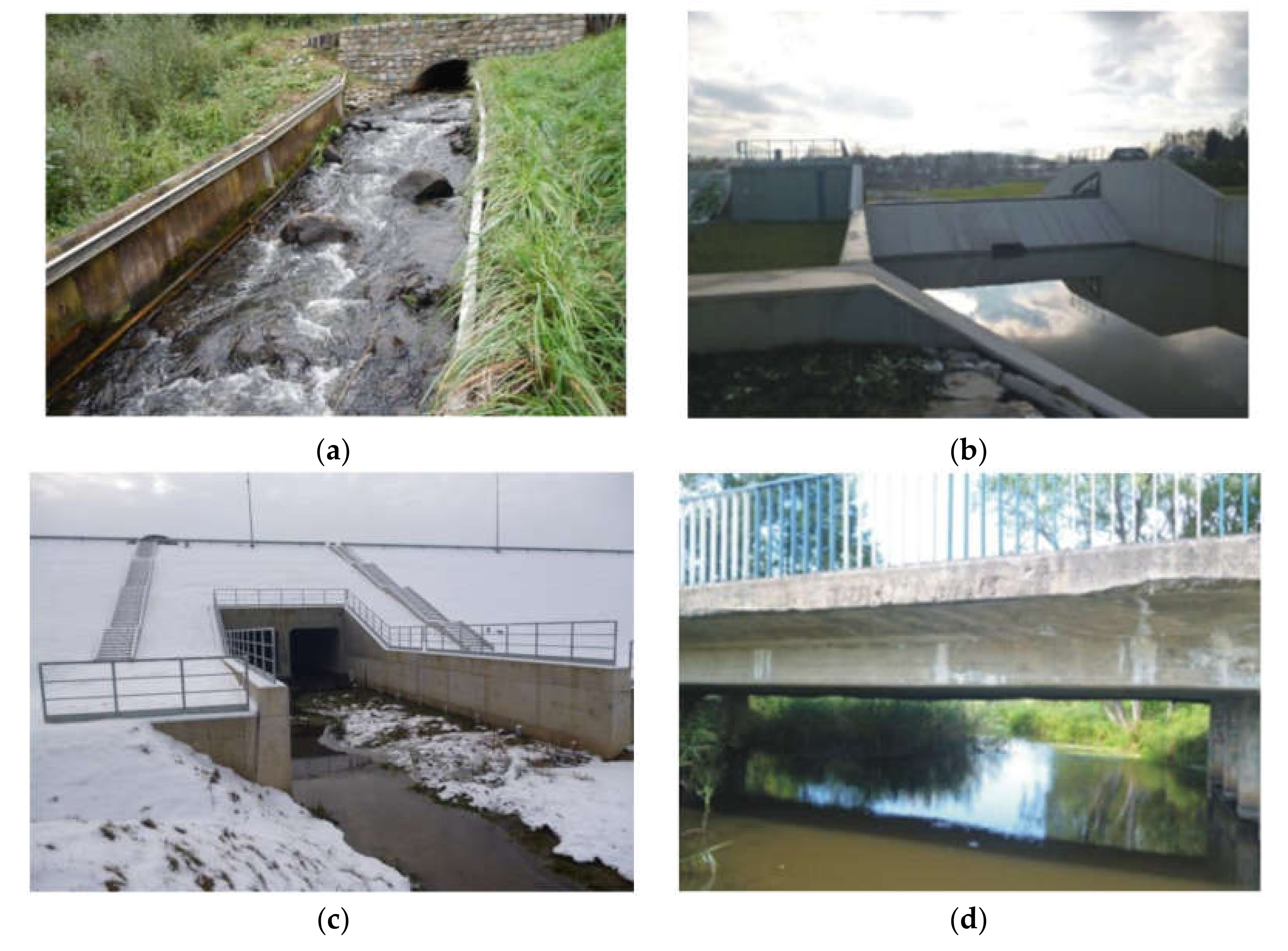
The objective of this paper is to develop a new empirical model for calculating peak discharge, expressed in terms of median of annual peak discharges (Q_MED) in the Upper Vistula basin within Poland. This region has the highest level of water resources in Poland, but it is also a flood risk area. The proposed empirical model can be used to assess the design discharge for designing different hydraulic structures like culverts, bridges, weirs, and orifices in small reservoirs (see Figure 1).

2. Materials and Methods

2.1. Study Area

The study was performed for 26 catchments located in the Upper Vistula basin (see Figure 2). In this region, the highest precipitation is observed. The annual maximum daily precipitation most frequently occurs between May and September and may be caused by continuous precipitation occurring over a large area or by heavy rains of local reach only [23]. One has to consider that mountainous areas are typified by low infiltration capacity of soils and steep hillslopes, and they are responsible for the formation of surface runoff. The Carpathian basin is formed mostly by impermeable soils: soils originating from medium and heavy tills, cherozemic soils and alfisols derived from clay loams and silt loams, soils derived from loams of different origin, soils derived from silts of different origin, and soils derived from silts, clays, and loams [8]. The main land cover is woodland and semi-natural ecosystems (on average, 55%) and arable land (on average, 39%). Urbanized areas occupy, on average, 5% of the studied catchment. The remaining part (1%) comprises wetlands and bodies of water. In this study, all analyses were performed for the catchments listed in

Table 1. Values of attributes of catchment characteristics located in the Upper Vistula basin.

Catchment Code	River – Cross-Section	A	H	St	Ss	Pi	Si	F	N	LHP	QMED
		(km2)	(–)	(–)	(–)	(–)	(–)	(–)	(–)	(–)	(m3·s−1)
C1	Prądnik – Ojców	67.5	0.7	−0.9	0.3	0.0	1.0	0.4	−1.3	1.2	1.2
C2	Uszwica – Borzęcin	268.5	−0.3	−0.7	0.6	0.0	1.6	0.5	−0.1	5.6	89.5
C3	Stobnica – Godowa	335.8	−0.4	−0.6	1.2	0.0	1.3	0.7	0.0	7.5	57.5
C4	Wapienica – Podkępie	52.7	−0.5	−0.2	1.6	0.5	1.3	0.6	−1.3	8.8	24.7
C5	Wisła – Wisła	53.4	0.0	0.0	2.9	1.0	0.7	1.1	0.6	20.1	23.4
C6	Bystra – Kamesznica	49.2	−0.2	0.0	2.3	0.9	0.8	0.7	0.8	16.5	10.7
C7	Żabniczanka – Żabnica	23.39	−0.4	0.0	1.5	1.0	0.6	1.1	0.7	15.2	8.6
C8	Wieprzówka – Rudze	151.8	−0.4	−0.6	0.2	0.2	1.4	0.5	−0.7	4.3	59.3
C9	Stryszawka – Sucha	140.0	−0.4	−0.8	−0.2	0.8	1.0	1.0	0.2	7.0	35.2
C10	Skawica – Skawica Dolna	143.8	−0.2	−0.6	−0.2	0.8	0.8	1.2	0.2	7.9	41.2
C11	Krzczonówka – Krzczonów	93.0	−0.3	−0.8	−0.4	0.2	1.1	0.9	−0.3	3.0	35.8
C12	Lubieńka – Lubień	48.1	−0.4	−0.9	−0.3	0.0	1.1	0.7	−0.1	1.8	12.8
C13	Skawa – Jordanów	123.7	−0.6	−0.9	−0.7	0.0	1.6	0.6	−0.3	1.2	26.5
C14	Raba – Rabka	102.0	−0.3	−0.9	−0.1	0.0	1.3	0.7	−0.5	2.2	23.2
C15	Mszanka – Mszana Dolna	174.0	−0.5	−0.7	−0.3	0.5	1.0	0.7	0.1	4.0	67.3
C16	Dunajec – Nowy Targ	685.1	0.0	−0.7	0.2	0.5	1.2	0.5	0.2	6.6	135.0
C17	Białka – Łysa Polana	78.0	−0.3	−0.8	2.5	1.4	0.1	0.5	−0.1	12.7	33.3
C18	Ochotnica – Tylmanowa	109.0	−0.1	−0.8	−0.1	0.0	0.6	1.1	0.4	3.9	18.5
C19	Grajcarek – Szczawnica	75.4	−0.3	−0.6	−0.4	0.0	0.6	1.3	0.3	3.7	15.3
C20	Kamienica – Nowy Sącz	237.7	−0.3	−0.8	−0.3	0.2	1.0	1.0	0.0	3.7	121.0
C21	Biała – Grybów	212.2	−0.8	−0.8	−0.6	0.0	1.2	0.9	0.2	2.3	77.0
C22	Wisłok – Puławy	143.6	−0.8	−0.6	1.1	0.5	1.1	1.3	0.4	11.7	53.3
C23	Osława – Szczawne	307.0	−0.8	−0.6	0.9	0.9	1.1	1.3	0.3	11.7	80.0
C24	Wetlina – Kalnica	131.2	−0.7	−0.5	1.2	1.0	0.8	1.6	0.2	13.3	45.9
C25	Czarna – Polana	113.8	−0.1	−1.0	0.9	1.0	1.2	1.3	0.5	13.2	26.8
C26	San – Zatwarnica	535.4	−0.4	−1.0	1.2	1.0	1.1	1.4	0.5	13.6	167.5

. In Table 1, the main characteristics of the analyzed catchments and attributes for the calculation of LHP are shown.

2.2. Landscape Hydric Potential

To identify the hydric potential of analyzed river catchments, the LHP method was used. The methodology of LHP calculation was described in detail by Lepeška [16], Lepeška et al. [18], and Wojkowski et al. [22]. The spatial distribution of LHP is the sum of all environment attributes and is calculated from Equation (1).

LHP = 1.5H + 2.5St + 3Ss + 4Pi + 3Si + 3.5F + 2N,

(1)

where H represents the attributes of hydrogeological characteristics, St represents the attributes of soil types, Ss represents the attributes of soil textures, Pi represents the climatic water balance, Si represents the attributes of slope inclination, F represents the attributes of the hydric effect of forest stands, and N represents the attributes of non-forest landscape.

The following steps of LHP calculation were used [18]: (1) the attributes, which describe the hydric potential, were scored based on the hydrologic quality of an area (landscape element/ecosystem); (2) the attributes were evaluated in relation to hydric potential of landscape; the ability and the quality of attributes with respect to retention and infiltrate precipitation, as well as quality of hydrometeorological attributes (precipitation and potential evapotranspiration), were evaluated; (3) the quality of attributes in relation to landscape hydric potential were graded as extraordinary (scores: +2.0; +2.5; +3.0), high (+0.5; +1.0; +1.75), moderate (0; in the category of forest stands +1.5), low (−1.0; in the category of forest ecosystems 0), very low (−2.0; −0.25), and limited (−3.0; −4.0); (4) attributes were weighted to show the importance attribute in relation to other attributes; (5) attributes were weighted in paired comparison of individual importance. Results were expressed by Fuller’s triangle. The following attributes were used for LHP calculation: hydrogeological characteristics H, which were chosen according to the level of bedrock transmissivity (T) based on of the Hydrogeological Map of Poland (HMP) in 1:50 000 scale; soil characteristics, which were estimated based on a soil vector map (SVM) developed with a soil agronomic map in 1:5000 scale; climatic water balance (Pi), which was calculated as a difference between annual precipitation and annual potential evapotranspiration; slope inclination (Si) assessment, which was based on a digital elevation model (DEM) with a 25-m resolution; non-forest landscape areas (N), which were identified with use of the land cover mapping within the CORINE Land Cover 2012 program; forest stands (F), which were evaluated on the basis of a report on the state of the Polish forests. The landscape attributes were superposed and scored within a GIS environment. The spatial analysis and data processing were realized by ArcGIS 10.0 software.

2.3. Hydrometeorological Data

The hydrometeorological data (daily sum precipitation, daily air temperature, and annual maximum discharges) covering the years 1971–2015 were obtained from the Institute of Meteorology and Water Management of the National Research Institute in Warsaw. Based on annual maximum discharges, a time series for each catchment median was calculated.

2.4. Statistical Analysis

Catchment area A and LHP were chosen to create empirical models for assessing Q_MED. Based on the A and LHP values, correlation matrices were determined in order to enable the initial selection of predictors to the formulas allowing estimation of Q_MED in ungauged catchments of the entire Upper Vistula basin. A multiple regression was used to build the model, the linear form of which is expressed by Equation (2).

Q_MED = a + b₁A + b₂LHP,

(2)

where Q_MED is the median of annual peak discharges (m³·s⁻¹), a is the regression constant (intercept), A is the catchment area (km²), LHP is the landscape hydric potential, and b₁, b₂ are coefficients of regression.

Statistical verification of the model was carried out for the significance level of α = 0.05. This consisted of checking whether assumptions were met, regarding the significance of regression equation, the significance of partial regression coefficients, the evaluation of redundancy between independent variables, and the verification of homoscedasticity of residues (residual scattering analysis, the normality of residual distribution, and the estimation of the expected value of the random component). Finally, based on the Nash–Sutcliffe coefficient (E) [24], the quality of the model was assessed. For assessing the quality of the model, Ritter and Muñoz–Carpena [25] criteria were used. According to these authors, E < 0.65 is deemed a lower threshold representing unsatisfactory performance. Other model performance ratings were as follows: acceptable (0.65 ≤ E < 0.80), good (0.80 ≤ E < 0.90), and very good (E > 0.90).

3. Results and Discussion

The research conducted by Młyński et al. [8] stated that the catchments in Upper Vistula basin are not characterized by statistically significant trends. Therefore, in the analyzed multi-year period, no factor appeared that would significantly affect the course of processes shaping flood flows from these catchments. Similar research results related to the analysis of changes in the flood flows from the catchments of the Upper Vistula river basin were presented in the papers by Wałęga et al. [26] and Kundzewicz et al. [27], where, in the majority of the studied cases, there were also no statistically significant trends found in the observation series of flood flows in the Upper Vistula basin.

As mentioned above, the LHP is a measure of potential water storage capacity of catchment, which includes many catchment characteristics. The LHP could be used as a descriptor to reflect water storage. Figure 3, Figure 4, Figure 5, Figure 6, Figure 7, Figure 8 and Figure 9 present the spatial characteristics of attributes that influence LHP value. It is clearly visible that analyzed catchments have high variability of characteristics. Bedrock transmissivity can influence soil infiltration. In the case of analyzed catchments, it is visible that attributes of hydrogeological characteristics range mostly from −1.0 to 0.0. 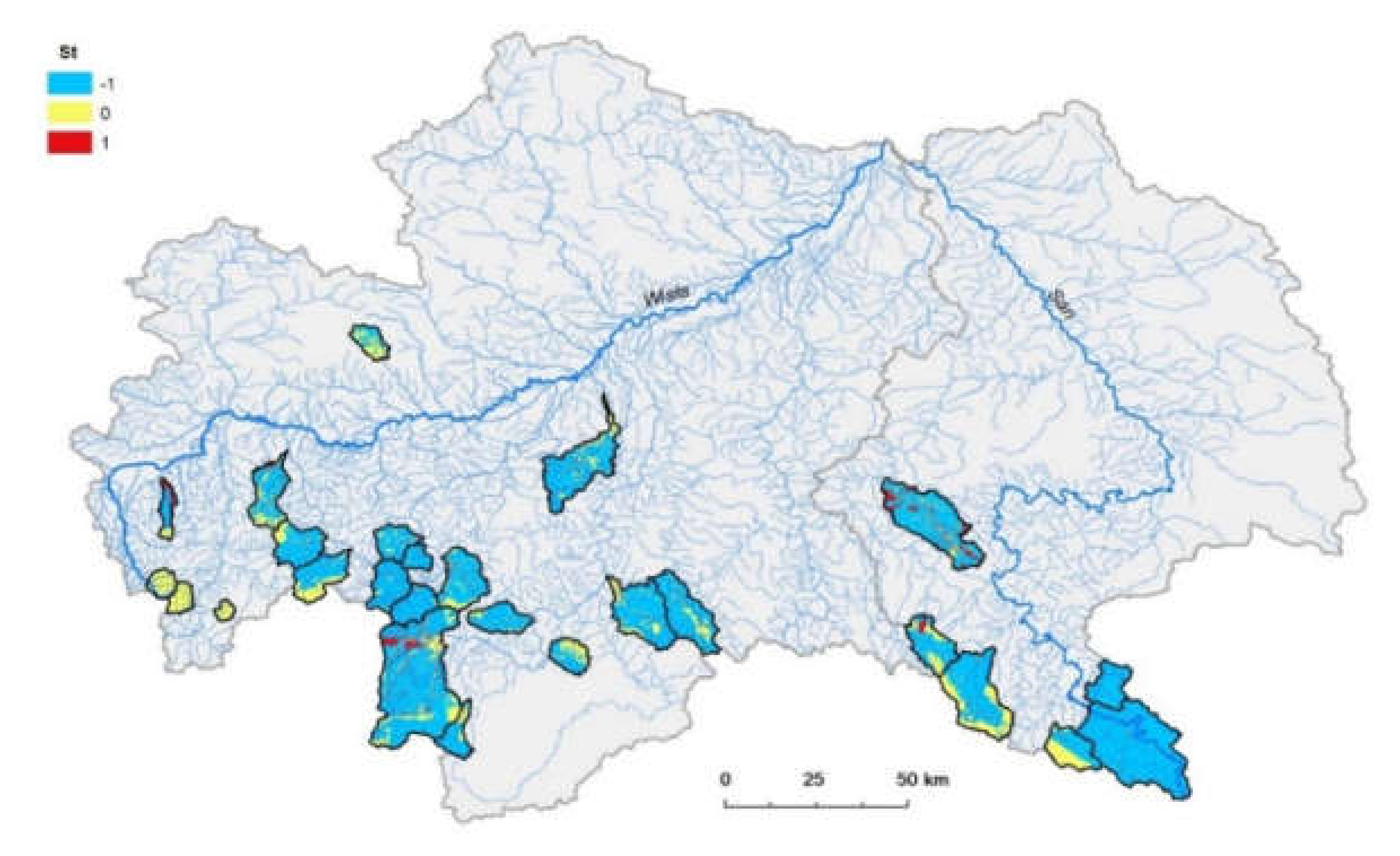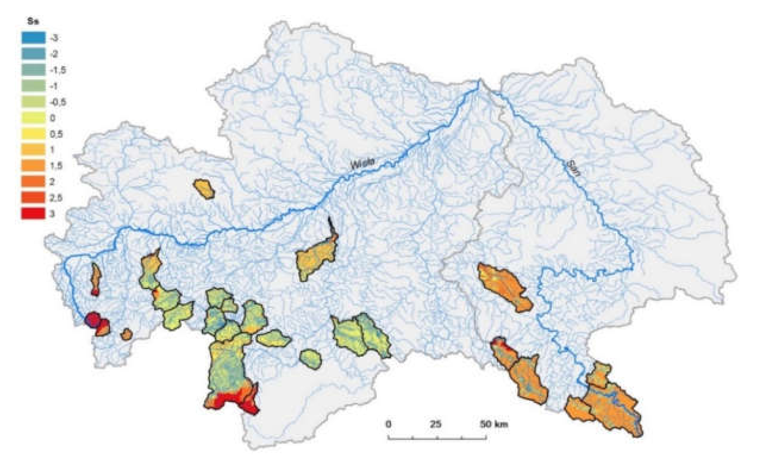Analyzed catchments with medium transmissivity (T = 1.10⁻⁴ to 1.10⁻³ m²∙s⁻¹) are formed particularly by marls and marly limestones (0.0 points), and catchments with low transmissivity (T < 1.10⁻⁴ m²∙s⁻¹) are formed mostly by granites or granodiorites (−1.0 points). Moreover, it is visible that catchments located in the south part of the Upper Vistula basin have lower transmissivity than catchments located in the lower part of the Upper Vistula basin. Soil texture (Ss) and soil type (St) also significantly influence the water infiltration [28]. In the analyzed area, the following soil texture classes are dominant: loamy sands (+2.0 points); sandy loams (+1.0 points); loams (0.0 points); clay loams (−1.0 points). According to the soil retention capacity, the dominant low (−1.0 points) categories of soil types (St) were divided into three categories. Therefore, low soil texture plays a key role in the formation of surface runoff, with an influence on a higher variety of discharges.

All mentioned conditions promote low water retention in mountain catchments. Furthermore, differences in the soil properties influence changes in land use, according to Lizaga et al. [29]. In consequence, changes in the soil properties are reflected in the hydric potential, and they influence the hydrological regime.

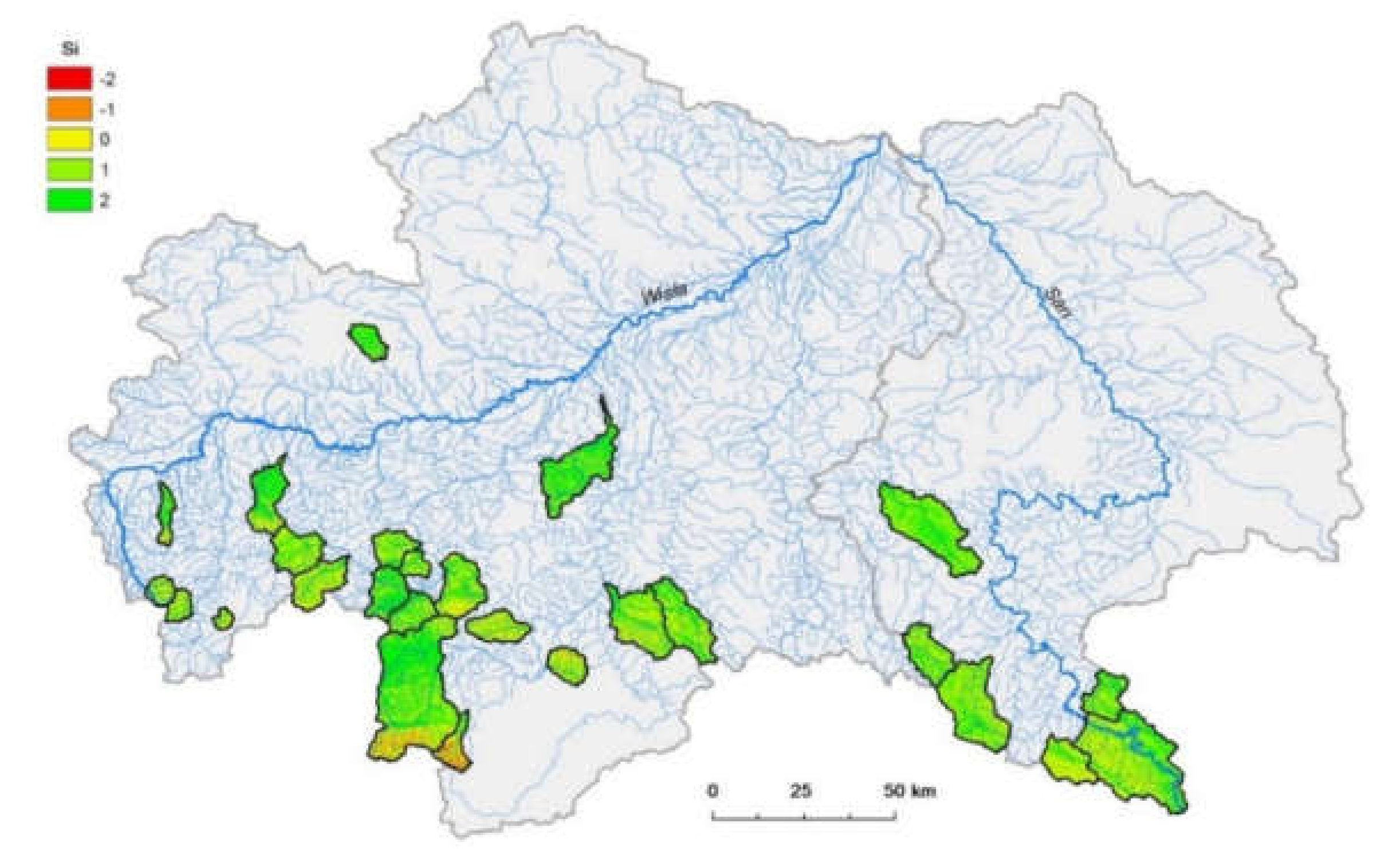
Slope inclination (Si) significantly influences infiltration intensity and the detention of rainfall. Generally, it could be said that infiltration intensity decreases with increasing slope inclination and surface runoff increase [22]. From Figure 6, it is clearly visible that slope inclination in analyzed catchments can promote a fast catchment response to rainfall because catchment slopes are mostly high, classified with the following attributes: Si 18.1°–31.0° (0.0 points); Si 31.1°–50.0° (−1.0 points); Si > 50.1° (−2.0 points). In catchments with a mild slope, Q_MED will significantly differ from that observed in mountain catchments. A mild slope will be caused by moderate discharge, because the time of concentration will be shorter than in mountain catchments. A good example of the influence of slope catchment on peak discharges is visible where the SCS-UH model is used. Blair et al. [30] suggested that a peak rate factor of 200 in the mentioned model is more representative than the default value of 484 recommended in the peak discharge method they used [12] for the flat terrain of catchments. The peak rate factor is a constant, intended to reflect the slope of the watershed, and it ranges from 600 in steep areas to 100 in flat swampy areas [12,31].

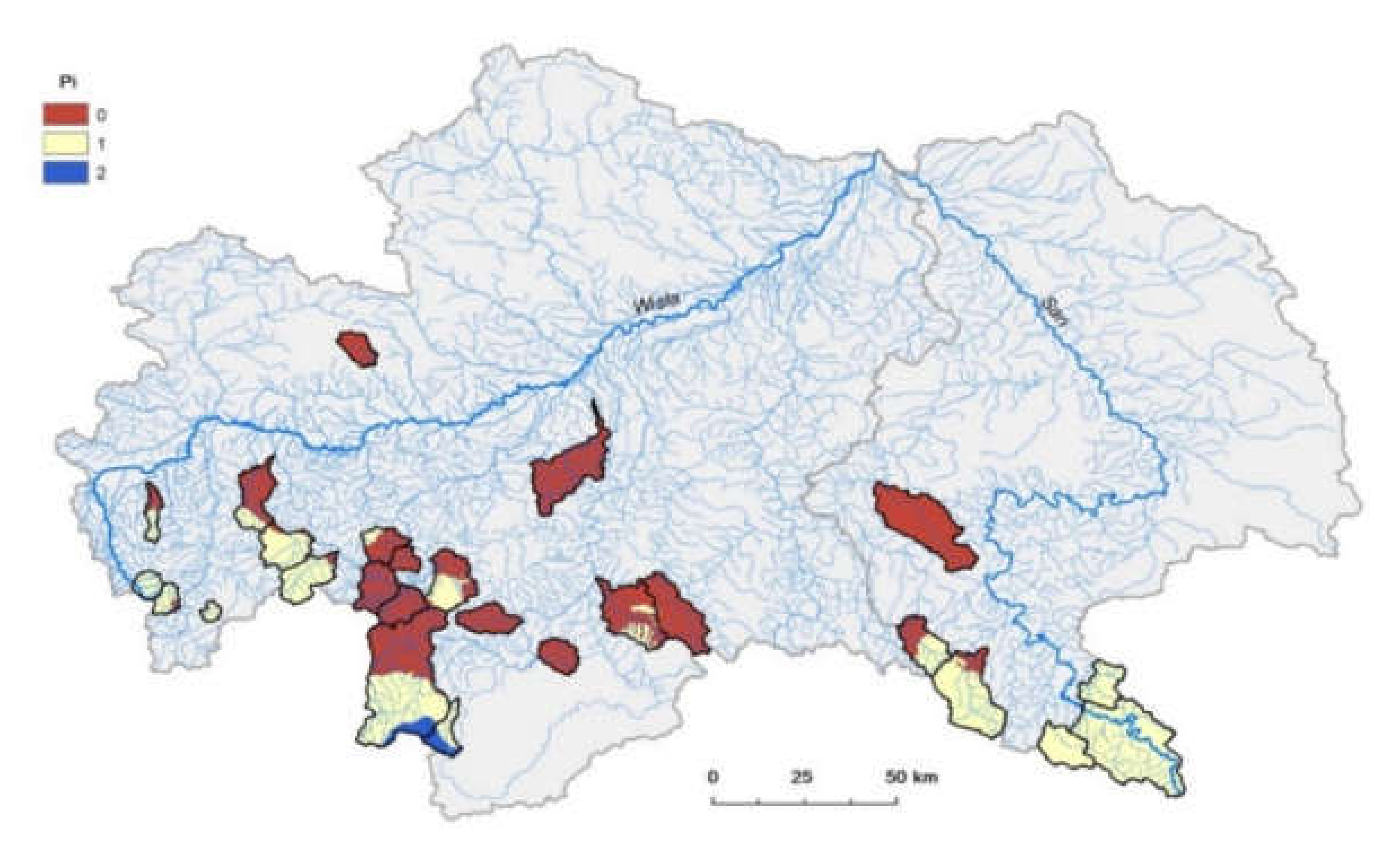
From Figure 7, it is visible that catchments located in the analyzed region have a positive climatic water balance. Pi attributes range from 0.0 points to 2.0 points. This suggests that precipitation is significantly higher than evaporation losses. Regarding the 2.0 attribute, climatic water balance is higher than 1100 mm, while that for 1.0 point Pi is between 451.1 and 1100 mm, and that for 0.0 point Pi ranges between 0.1 and 450.0 mm. Catchments located in higher altitude mainly have more visible positive climatic water balance. 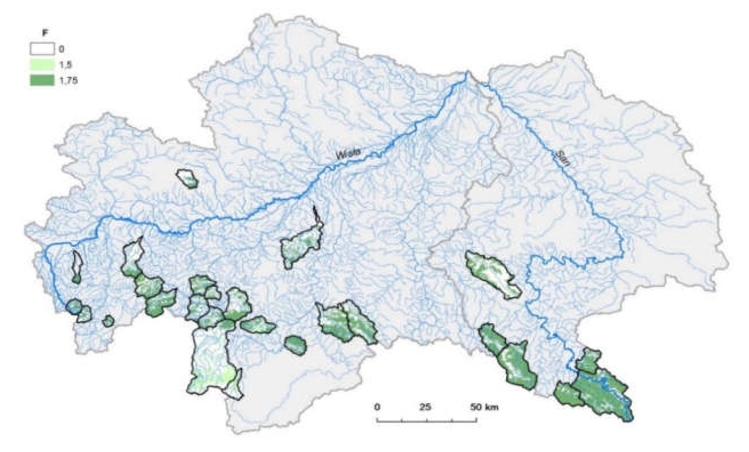These catchments have the highest flood potential because soil is less permeable, and higher catchment slopes promote faster runoff because they have lesser water storage [32]. In the case of land cover, analysis was divided into two parts, first with regard to forest cover and second with regard to the remaining types of land cover. The forest plays an essential role in water balance and water quality. In forest catchments, a low gradient is mainly observed, due to saturated runoff or subsurface drainage (runoff) that occurs later than surface runoff [33,34]. In the analyzed mountain catchments, forest stand attribute F varied greatly. In the Bieszczady Mountains (catchments 23−26) better forest quality was observed than in the remaining catchments (see Figure 8). In those catchments, the F attribute was highest, equal to 1.75 (ecosystems of great stability). In the case of the Dunajec river (C16), the lowest F attribute, equal to 0.0 (unstable ecosystems), was observed. One of the main reasons is the deforestation problem that caused higher runoff with an influence on the change in concentration of ions in water [35,36]. Generally, the deforestation of Dunajec catchments influenced the lowest LHP, equal to 6.6 (see Table 1). 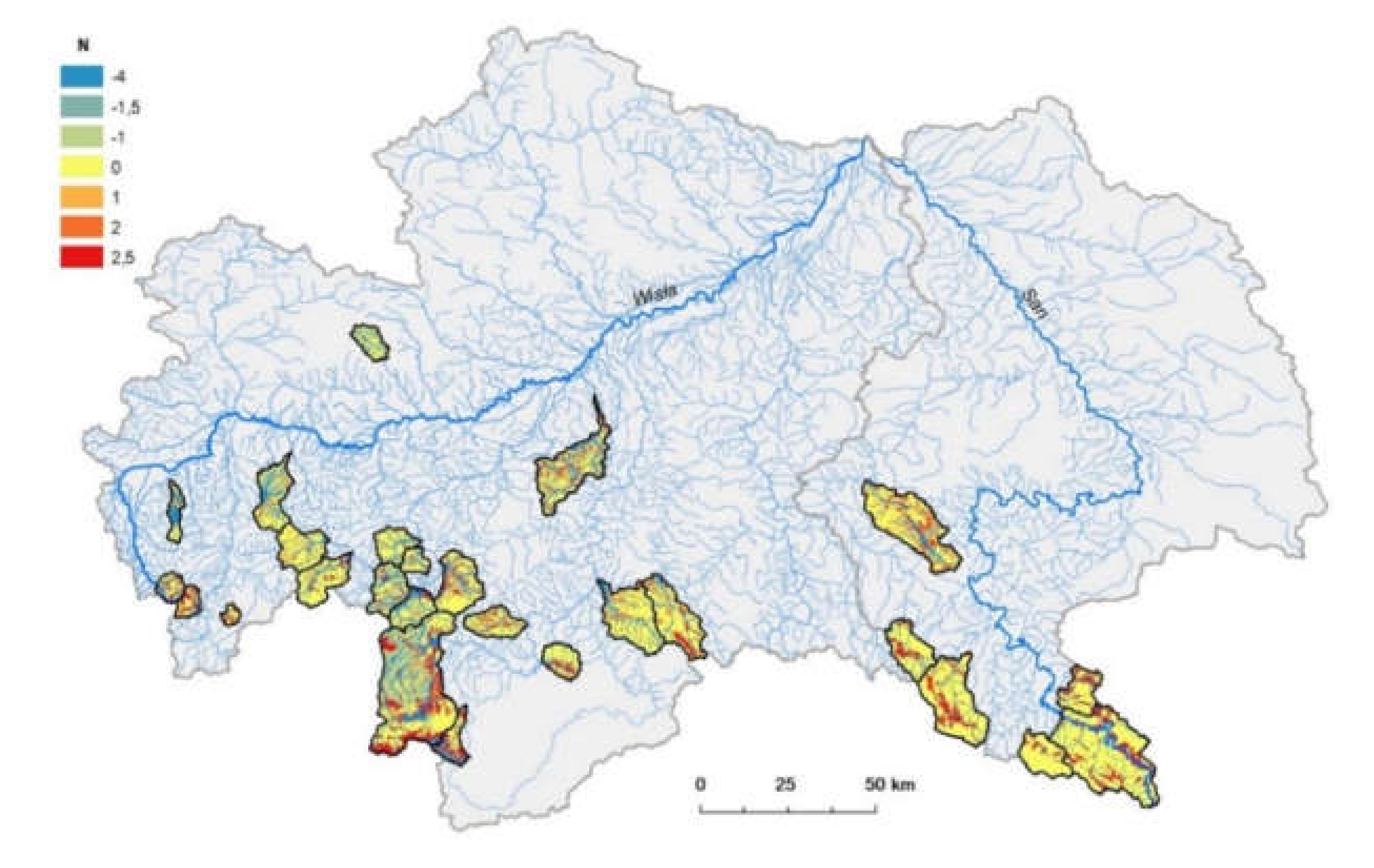Figure 9 illustrates non-forest landscape (N) characteristics. In the analyzed catchments, the following landscape types dominated: complex of fields, grasslands, and permanent crop areas (+1.0 points) and arable land (−1.0 points). These land cover types are typical with lower water storage and faster catchment response to rainfall. It seems that landscape hydric potential adequately describes the process of shaping the outflow from the basin in empirical models used in estimating peak discharges, instead of using many variables describing the individual features of the catchment. Such synthetic indicators are used, inter alia, to describe design hydrograms. LHP values for each catchment are presented in

Table 2. Basic statistical parameters of analyzed variables.

Parameter	Min*	Mean	Median	Max	s	Cs	Ske	K
A	23.39	167.55	127.45	685.08	152.45	90.99	2.24	5.34
LHP	1.20	8.39	7.25	20.10	5.46	65.10	0.47	−0.96
QMED	1.19	49.62	35.40	167.50	41.42	83.46	1.40	1.67

*Min—minimum, max—maximum, s—standard deviation, C_s—coefficient of variation, Ske—skewness, K—kurtosis.

. The LHP value varied from 1.2 Skawa (C13) and Prądnik (C1) to 20.1 for Wisła (C5). Catchments with low LHP have reduced possibility of water retention, which is caused by low soil permeability and higher slope inclinations. On the other hand, these features are buffered by high forest cover, which influences higher LHP, as in the case of Wisła (C5), Bystra (C6), or Białka (C17). Although these catchments have mountainous characteristics, higher water storage capacity is visible. 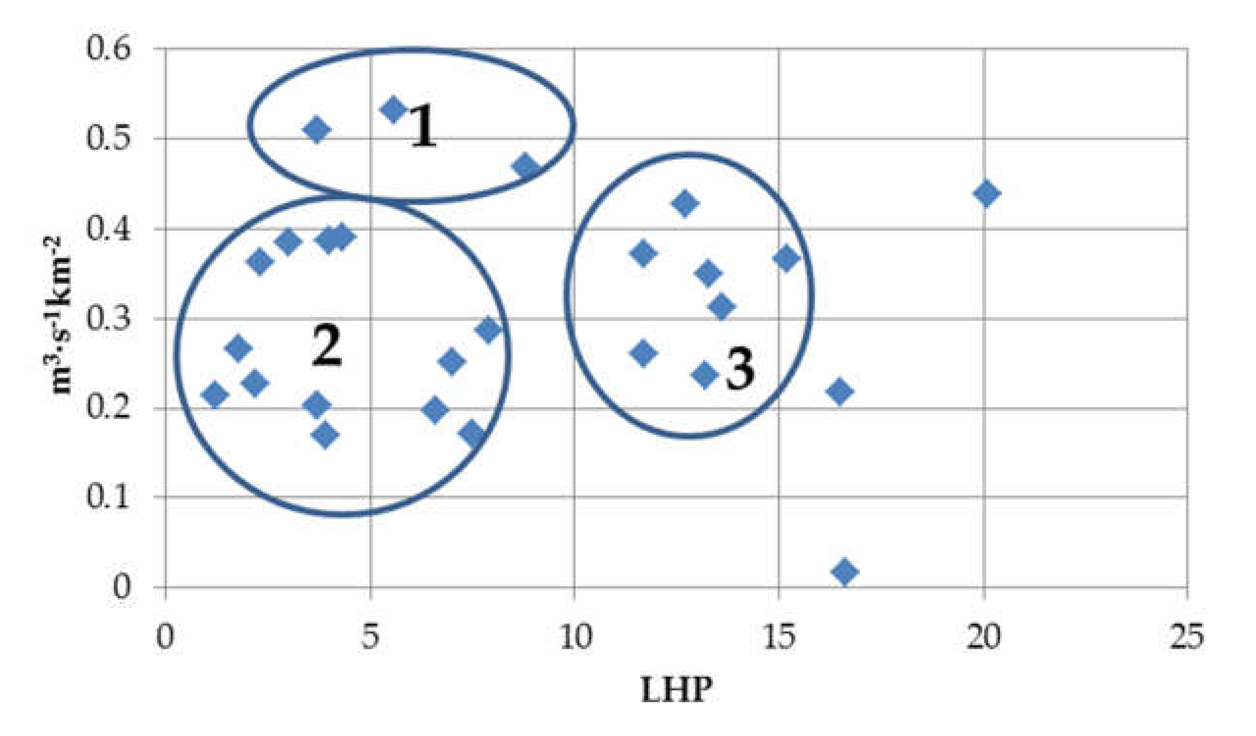In Figure 10, the relationship between LHP and rate of median outflow Q_MED is not clearly visible, but three main clusters and three additional points can be differentiated. The first cluster has three catchments, Uszwica (C2), Kamienica (C20), and Wapienica (C4), with a rate of discharge above 0.46 m³∙s⁻¹∙km⁻². These catchments are characterized by relatively low LHP. As mentioned earlier, low LHP is observed for catchments with low infiltration and relatively lesser forest cover in comparison to the rest of catchments. This situation supports a faster response of catchments to rainfall events and, thus, higher discharges. The second cluster has catchments with lower LHP and lower peak discharge rate. In these catchments, forest is the dominating type of land cover and, thus, water retention is higher, which additionally buffers the disadvantageous effect of hydrogeological and geomorphological conditions like slope inclinations on runoff. The third cluster has catchments that are characterized by higher LHP but peak discharge rates similar to the second cluster. Higher LHP is mainly influenced by higher forest cover in this region of Poland. This influences the lower peak rate. Higher LHP is influenced by a slightly lower slope inclination than that observed in catchments grouped in the second cluster. The last two catchments, i.e., Wisła (C5) and Prądnik (C1), have the highest and lowest LHP, respectively. In the case of Prądnik river, the peak discharge rate is the lowest in comparison to the remaining catchments. In this case, discharges are moderated by the influence of artificial ponds located in the upper part of the catchment and karst areas. 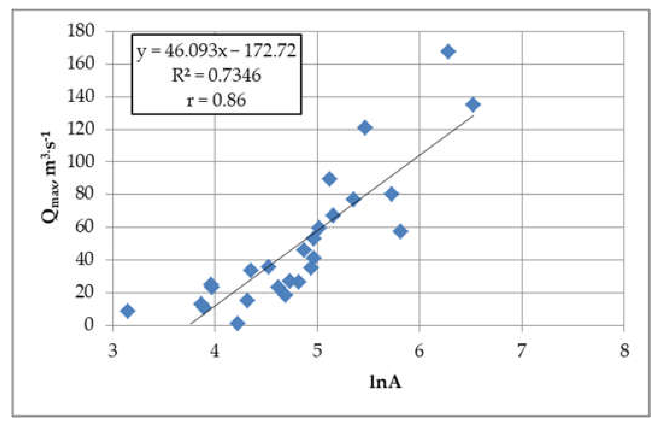Moreover, a higher LHP value is observed in the Wisła (C5) catchment, with a higher peak discharge rate equal to 0.43 m³∙s⁻¹∙km⁻². The higher peak rate is influenced by the higher precipitation in comparison to the Prądnik river. The catchment area was selected as the second parameter in the proposed model. As shown in Figure 11, relationships between catchment area and peak discharges are clearly visible. In further analysis, the catchment area was recalculated and expressed as the logarithm of area.

Table 2 shows the basic statistical parameters of the analyzed variables. The mean catchment area is equal to 167.55 km² with the minimum value equal to 23.39 km² and the maximum value equal to 685.1 km². The mean LHP value is equal to 8.39 with a range of 1.2 to 20.1. The Q_MED mean value is equal to 49.62 m³·s⁻¹ and with a high range of values from 1.19 to 167.5 m³·s⁻¹. Based on the coefficient of variation, it was concluded that LHP and Q_MED values were characterized by high and very high variability in the analyzed period. This was due to the alteration of years with very high and very low precipitation. The 1980s belonged to a relatively dry period. At that time, practically throughout Poland, a significant lowering of the groundwater was observed, which contributed to the reduction of discharge in rivers. However, the years 1997, 1998, and 2010 were extremely wet periods, during which precipitation occurred, leading to catastrophic floods [37].

Simple correlation analysis showed that the correlation coefficient r between Q_MED and lnA was 0.86 and its statistical significance had a p-value = 0.000; r between Q_MED and LHP was equal to −0.124 (not significant, p-value = 0.547), while the correlation coefficient between lnA and LHP was equal to 0.25 (not significant, p-value = 0.210).

Table 3. Results of the significance analysis of linear regression model and the significance of the component coefficients of regression for the model for estimating Q_MED throughout the Upper Vistula basin.

Variable	F	p	b*	Standard Error of b*	b	Standard Error of b	t	pi
a	33.434	0.000			−185.72	31.09	−5.97	0.000
lnA			0.883	0.109	47.46	5.87	8.09	0.000
LHP			0.100	0.109	0.761	0.83	0.92	0.367

F—Fisher–Snedecor distribution; p—p-value for the regression model; a—value of the absolute term; b*—normalized coefficient of regression; b—coefficient of regression; t—quotient b/(standard effort of b); p_i—p-value for partial coefficients of regression models.

presents the results concerning the analysis of the significance of the linear regression of the model and the significance of partial regression coefficients.

Based on the values summarized in Table 3, it is visible that the empirical model for assessing Q_MED in the mountain catchments of the Upper Vistula basin is characterized by a statistically significant value of the F statistic, for which the p-value is less than the assumed significance level of α = 0.05. In turn, statistically significant values of p_i partial regression coefficients occur for the catchment area. Of course, the LHP variable does not have a significant influence on the model but it was decided that this statistically insignificant parameter should be retained, because LHP includes all factors essentially influencing water storage capacity. Furthermore, LHP is influenced by climatic conditions like precipitation and evapotranspiration. Precipitation and evaporation are input parameters in water balance, and they influence the volume of runoff from catchments. Another reason to include LHP in the model is land cover. As mentioned earlier, non-forested and forested areas play an important role in the response of catchments to rainfall and in shaping water storage capacity. Generally, including LHP in the proposed model can provide calculations in changing climate conditions and land use. Finally, the shape of the proposed model was established using Equation (3).

Q_MED = −185.72 + 47.46∙lnA + 0.761∙LHP (m³·s⁻¹),

(3)

where A is the catchment area (km²), ln is the natural logarithm, and LHP is the landscape hydric potential.

The proposed model is based only on two variables: catchment area and LHP. According to Węglarczyk [38], the number of predictors describing the dependent variable should not be overly high. This is due to the fact that each independent variable, in addition to information about the forecasted value, carries with it a certain degree of uncertainty, resulting from the observation series of this particular feature.

The correlation coefficient of the proposed model is equal to R = 0.862 and is statistically significant for α = 0.05. The coefficient of determination R² is equal 0.722. In the next step of verification of the proposed model, the tolerance factor was calculated. When the value of this factor is higher than 0.1, it can be concluded that there is no collinearity of independent variables. The results of this analysis are summarized in

Table 4. Results of the collinearity analysis of independent variables in the studied forms of the model for determining Q_MED in the mountain catchments of the Upper Vistula basin.

Variable	Tolerance Factor	r2c	Partial Correlation	Semi-Partial Correlation
lnA	0.935	0.064	0.860	0.854
LHP	0.935	0.064	0.188	0.097

r²_c—value of the coefficient of determination between the given variable and all other independent variables.

.

As can be seen from Table 4, it was found that the tolerance for all variables was high (above 0.1). In addition, the values of coefficient r²_c differed significantly from one. Thus, the independent variables did not show redundancy in regression equations, which indicated the lack of their collinearity.

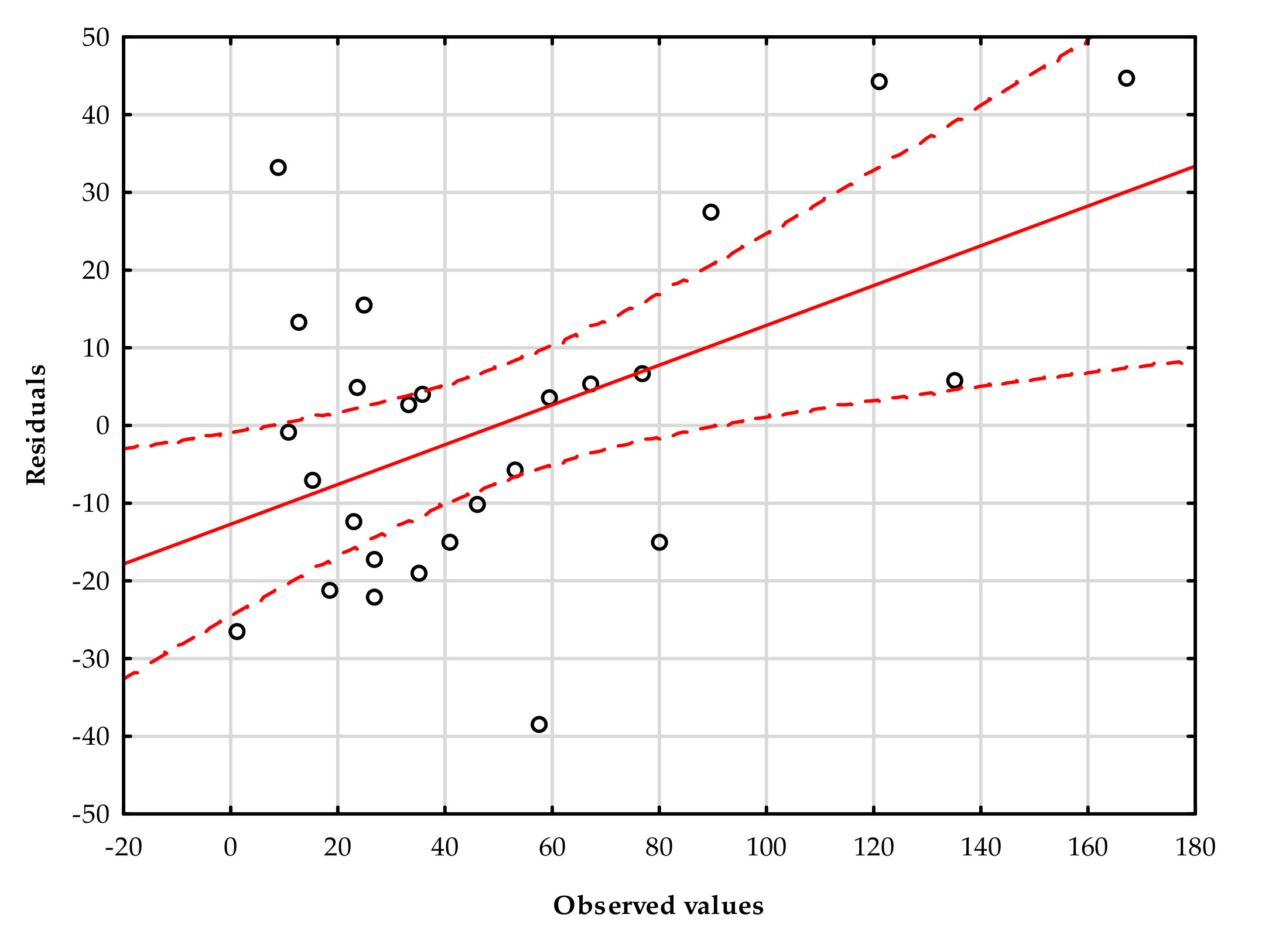
The assumption of constancy of the variance of the random component for individual values of independent variables was verified using scatter plots. Figure 12 presents predicted values relative to residual values.

In Figure 12, the lack of heteroscedasticity (violation of the assumption of homoscedasticity) of the random variables being analyzed is clearly visible. Points on the graph are arranged in the form of an evenly distributed cloud, and there are no clear systems of the points that form individual groups. Therefore, there is no reason to reject the assumption of constancy of the random component variance for individual independent variables.

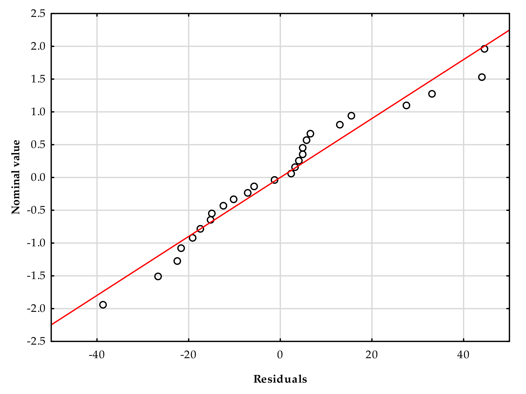
The normality of the distribution of residues was verified using a normality plot (see Figure 13). In this figure, a chart of nominal (expected) values relative to residual values obtained by applying the tested form of the empirical model is presented. Based on the normality plot of the residuals, it was found that, for the analyzed equation, most points are arranged along a straight line. Hence, the inference was that, in these cases, the distribution of residues is consistent with a normal distribution.

The final verification of proposed model was performed based on the scatter plot in Figure 14, which presents Q_MED observed discharges versus those calculated with the use of Equation (3). It is visible that, for lower values of Q_MED, the proposed model adequately predicted peak discharges for the most part. The Nash–Sutcliffe coefficient (E) of efficiency was equal to 0.774; thus, according to the previously discussed criteria [25], the proposed model has good quality.

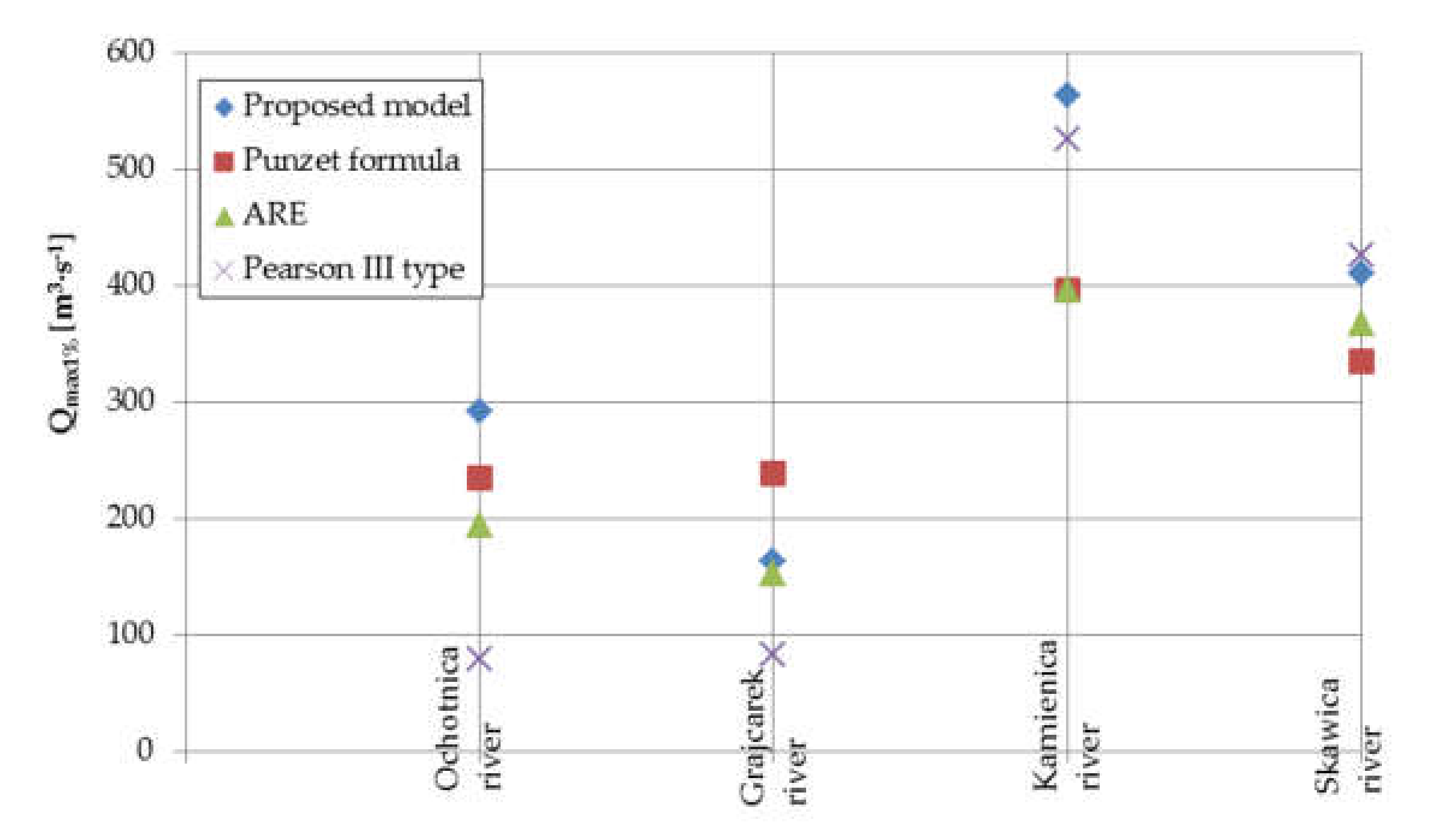
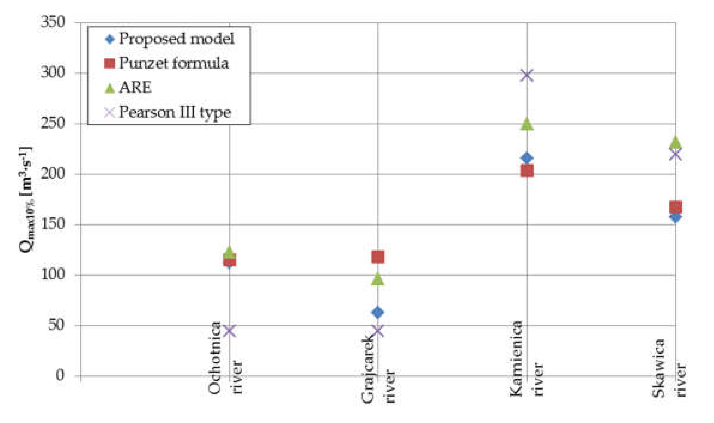
Figure 15 and Figure 16 show a comparison of peak discharges with probability equal to 1% and 10% assessed using the proposed model, Punzet formula, and spatial regression equation (ARE) for four catchments. Additionally, the figures show the same discharge assessment based on Pearson type III distribution for the observed time series. This distribution is recommended in Poland to assess design peak discharges. Peak discharges for the 1% probability assessment based on the proposed model were higher than the assessment based on Pearson type III for Ochotnica (C18), Grajcarek (C19), and Kamienica (C20) river. Differences were mainly visible for Ochotnica (C18) and Grajcarek (C19). In the case of the last two catchments, peak discharges from the proposed model were close to those achieved for Pearson type III distribution (PIII distribution). In comparison to other empirical models commonly used in Poland, the proposed model gave higher values of peak discharge. This is an important conclusion because commonly used models like Punzet or ARE were created in the 1970s or 1980s, where climatic conditions and land cover were different from those which occur now. Therefore, higher values of peak discharge accomplished by the proposed model can give safer values of discharge and, thus, safer parameters of hydraulic structures. In the case of the 10% probability assessment, the proposed model underestimated discharges in comparison to PIII distribution, and other models for Kamienica (C20) and Skawica (C10) river slightly overestimated discharges in comparison to the PIII distribution for Ochotnica (C18) and Grajcarek (C19) river.

4. Conclusions

The objective of this paper was to develop a new empirical model for calculating peak discharge, expressed in terms of the median of annual peak discharges (Q_MED) in the Upper Vistula basin in the Polish Carpathians. Landscape hydric potential (LHP) is an essential parameter representing the novelty of the proposed model. The proposed method is simple contrary to others which are used at the moment, and it might be very useful for river catchment managers, especially in places where fast decisions are needed for catchment intervention. The LHP parameter was not previously used as a component in hydrological models. LHP is based on the assessment of the average amount of precipitation and on landscape attributes influencing runoff infiltration, deceleration, and retention, hydrogeological characteristics, soil type and soil texture, climatic water balance, geomorphologic conditions, and land cover. Thus, as shown in this paper, LHP includes all factors essentially influencing water storage capacity. If LHP were included in proposed model, it could provide a calculation for climate and land use changes. The proposed model is not complicated to use since it needs only two parameters for calculating Q_MED: catchment area and LHP. This method uses GIS techniques, allowing users to quickly include a lot of information with an essential role in runoff formation. In this case, the proposed model has quite a large advantage when comparing it to commonly used methods at present, since it includes the spatial distribution of soil, hydrogeology, geomorphology, and land-use characteristics in the catchment in a more appropriate way. Because the model has a significant and high correlation coefficient, as well as high quality, it could be used for assessing Q_MED in ungauged mountain catchments in the Upper Vistula basin in the Polish Carpathians. In comparison to commonly used empirical models at present, which include more complex parameters, the model proposed here is simple and clear, and it is useful for practitioners in water resource management. Using LHP based on catchment properties and on the most recent hydrometeorological data is a strong advantage of the proposed model.

Finally, the new model for assessing design peak discharges gives more precise results than commonly obtained from empirical models. The proposed model could be used by river catchment managers, engineers for designing hydraulic structures (e.g., culverts, small bridges, weirs, and orifices in small reservoirs in mountain catchments of Carpathian region), and reclamation engineers. The model can be applied in the Upper Vistula basin, for catchments with a surface area ranging from 24 km² to 660 km².

Future research should be focused on testing the proposed model in other catchments in different regions of Carpathian countries to verify it, especially in catchments with mild and very high slopes.