Performance Investigation of the Immersed Depth Effects on a Water Wheel Using Experimental and Numerical Analyses


1
College of Water Conservancy and Hydropower Engineering, Hohai University, Nanjing 210098, China
2
College of Energy and Electrical Engineering, Hohai University, Nanjing 210024, China
*
Authors to whom correspondence should be addressed.
Water 2020, 12(4), 982; https://doi.org/10.3390/w12040982
Submission received: 15 February 2020
/
Revised: 18 March 2020
/
Accepted: 25 March 2020
/
Published: 30 March 2020
(This article belongs to the Section Hydraulics and Hydrodynamics)
Abstract
:The purpose of this research is to study the effect of different immersed depths on water wheel performance and flow characteristics using numerical simulations. The results indicate that the simulation methods are consistent with experiments with a maximum error less than 5%. Under the same rotational speeds, the efficiency is much higher and the fluctuation amplitude of the torque is much smaller as the immersed radius ratio increases, and until an immersed radius ratio of 82.76%, the wheel shows the best performance, achieving a maximum efficiency of 18.05% at a tip-speed ratio (TSR) of 0.1984. The average difference in water level increases as the immersed radius ratio increases until 82.76%. The water area is much wider and the water volume fraction shows more intense change at the inlet stage at a deep immersed depth. At an immersed radius ratio of 82.76%, some air intrudes into the water at the inlet stage, coupled with a dramatic change in the water volume fraction that would make the flow more complex. Furthermore, eddies are found to gradually generate in a single flow channel nearly at the same time, except for an immersed depth of 1.2 m. However, eddies generate in two flow channels and can develop initial vortexes earlier than other cases because of the elevation of the upstream water level at an immersed radius ratio of 82.76%.
1. Introduction
Renewable energy gradually attracts people’s attention owing to the fact that there are huge demands for energy and an over reliance on conventional fossil fuels [1]. Hydropower resources are valued by all over the world for its clean, renewable and abundant characteristics [2,3]. To make full use of hydropower, different hydro turbines are generally chosen according to different heads. Meanwhile, hydraulic constructions are needed, such as pressured conduits, dams, reservoirs and so on [4,5]. So, they always need much time and huge investments. In recent years, low and ultra-low head-generating devices are increasingly popular as a number of large scale and capacity hydropower stations have been constructed [6,7]; it would be an effective way to use a water wheel to generate electricity in low and ultra-low head resources, such as open channels, streams and so on.
A traditional water wheel is known as a power source for grinding grains in watermills rather than electricity production [8]. It is generally believed to be a romantic but inefficient hydraulic machine today [9]. According to the characteristics of different waterwheels, the four main kinds of water wheel models are overshot, breast-shot, undershot and stream [9,10,11]. The stream wheel mainly uses kinetic energy, and the others mainly make use of potential energy. The overshot water wheel, which is recognized as the most effective traditional water wheel, is suitable for high heads. The water flows into cells at the top of the water wheel. The breast-shot water wheel, regarded as less effective than the overshot water wheel, is mainly applied in smaller heads than the overshot waterwheel. The water passes the water wheel approximately at the level of the axle. The undershot water wheel is suitable for very low heads. The water passes wheels under the axle of the waterwheel. The stream water wheel can be referred to as a substitutable waterwheel with only employing kinetic energy. Both the undershot and stream water wheel have been much less researched because of their worse performance.
However, with development of CFD (Computational Fluid Dynamics) and urgent demands for exploitation of ultra-low water resources, many researchers began to focus on those water wheels that are suitable for open channels, tidal current and rivers. Several experiments and numerical simulations were carried out to characterize the performance of water wheels. Emanuele Quaranta et al. [11,12,13,14,15,16,17] mainly researched the performance of breast-shot and overshot water wheels coupled with different blade shapes, inflow configurations and numbers of blades through simulations and experiments, and analyzed the reasons of efficiency loss for overshot and breast-shot water wheels theoretically; the results showed an optimized shape had a more complicated design and those water wheels with 48 blades showed much higher efficiency than others. Furthermore, 48-blade wheels could also produce low turbulence intensity to make less of an effect on flow field. Moreover, the equations about the optimal number of blades were generalized based on the hydraulic and geometric conditions. For improving the performance of an undershot water wheel, the different blade shapes were studied; three different blade shapes (triangular, propeller and curved) were researched through experiments by Lie Jasa et al. [18]. The results indicated that a triangular blade shape performed at the highest efficiency, but it was seriously affected by install location. Yasuyuki Nishi et al. [19] carried out an experiment for two different runners with no bottom plate and those equipped with a bottom plate. The results showed that runners with no bottom plate had a better performance at high speeds because of receiving twice the amount of flow; meanwhile, no air bubbles were carried into the gap between the runners. In addition, Manh Hung Nguyen et al. [20] compared the different performances with three blade shapes (straight, curved and the similar to Zuppinger type) through numerical experiments for stream wheels. The study demonstrated that straight blades with a simple construction had a better efficiency; in addition, the same conclusions were made by Emanuele Quaranta et al. [15]. To better characterize the stability and flow characteristics for water wheels with different numbers of blades, Nguyen Manh Hung et al. [21] discussed fluctuation of water-level differences between upstream and downstream areas and the output for different numbers of wheels; it was found that the six-blade wheels generated a greater torque and the water-level difference would be elevated remarkably as the number of blades increased. Many other studies had also been researched for breast and undershot water wheels through experiments and simulations [22,23,24,25,26,27,28,29]. However, those researches cannot have a generalized conclusion; water wheels still need to be developed for improving their performances. In addition, an experimental study on the effect of channel width on water wheel performance was conducted by Shakun Paudel et al. [30]. The results demonstrated that reducing channel width upstream could remarkably improve output and efficiency, because it reduced turbulent loss and created supercritical flows downstream. Similar experiments were conducted by Ilaria Butera et al. [31]; for a better performance, they suggested that the minimum distance between the canal wall and the side of the wheel should be 0.3 times the width of the wheel. Experiments and numerical simulations were also contributed to study the environmental effects for floating and stream water wheels [32,33,34,35,36], which demonstrated that a trailing vortex may generate local erosion, but environmental effects may be minimal. In addition, Emanuele Quaranta [37] presented the guidelines for a stream water wheel. There were also some special turbines that were put forward for exploiting low and ultra-low resources. The savonius vertical turbine was brought up to extract energy from low current speeds in rivers and tidal currents. The savonius turbine mainly was applied in wind energy primitively; it is considered to be an effective hydro turbine for low heads because of the low cost and maintenance. Recently, researchers developed numerical analyses and experiments to improve the performance of the savonius vertical turbine [38,39,40,41,42,43]. It was found that the numbers of blades and the twist angle had a significant effect on the turbine’s performance; however, it still need to further its design to make it commercially work. In numerical simulations, the different turbulence models are adapted to different kinds of flow for improving accuracy. Dendy Adanta et al. [44] assessed the different turbulence models for numerical into water wheels through experiments; it was found the SST k-ω was recommended for breast-shot water wheels, but it did not constitute a final conclusion. Above all, those researches played an important role in exploiting low head resources and improving water wheel performance. However, some design parameters still were considered empirical [32,45,46,47,48,49,50]; lots of research still need to be done. Nowadays most of the water wheels that are designed and constructed still rely on experiences; furthermore, performance and flow characteristics are still unclear and have not been brought into consideration at different immersed depths; therefore, clearing the flow characteristics and improving knowledge of the performance of water wheels at different immersed depths have remarkable significance for further commercial work.
So, this paper is concentrated on studying the different immersed depth effects on performance and flow characteristics through numerical simulations. This research conducted the experiments at an immersed depth of 0.8 m based on a real-size model. The optimal immersed depth is identified. The results are expected to enhance the design and knowledge for stream water wheels.
2. Numerical Simulation Method
2.1. Simulation Model
The real-size stream water wheel is an 8-blade wheel of a straight-type considered a simple manufacture; diagonal blades will be designed for a better performance in the next researches. The flow depth is 2.2 m, the distance is 13 m from gate to the center of water wheels and the distance between the side walls is 11.4 m. In order to make full use of kinetic energy, the water wheel is designed with wheel breadth of 11.0 m, outer diameter D of 2.9 m, hub diameter d of 0.16 m and side clearance of 0.2 m. The 3D model of the water wheel was established using Unigraphics NX, mainly including the rational domain and flow domain. To ensure a fully developed water flow, the rotation domain is at the center of the flow domain with a length of 16.35D (40 m) and height of 2.37D (7.0 m) [15,23,51] through verifications.
2.2. Grid Division and Sensitivity Analysis
The grids play an important role in numerical simulation and are a representation of geometry. They also have a significant effect on the accuracy and efficiency of the numerical simulation. The hybrid grid is applied in this research with an unstructured tetrahedral mesh in the flow domain and hexahedral mesh in the rotational domain, generated by ICEM CFD. Figure 1 shows the geometric model and grids in the wheel domain.
For evaluating the performance of the water wheels at different rational speeds, the “tip-speed ratio” (TSR), λ, a non-dimensional parameter, is applied [52]. The λ is defined as
where = the water wheels’ radius (m), = the angular velocity the velocity of the inlet (m/s).
The efficiency is remarkably affected by TSR. In this research, different working conditions were simulated through changing different immersed depths and rotational speeds. The case of the water wheel’s output is verified for mesh dependence at an immersed depth of 1.0 m and TSR of 0.3037 (6 r/min), as presented in Figure 2. It could be concluded that the nearly 4 million elements are reliable as the torques keep stable. So, this number of the elements is chosen for different cases. In this case, the flow domain’s mesh dimensions range between 0.23 m (0.021D) to 0.12 m (0.011D) and the wheel domain’s mesh dimensions range between 0.12 m (0.011D) to 0.07 m (0.006D); local mesh refinements were generated near the blades, also, Y+, a non-dimensional wall distance, is about 34 at the blades [21].
In addition, for giving a better evaluation for the ability to extract energy in the stream, the power coefficient is used to describe the ratio of energy extraction by a water wheel to energy available in the stream. The power coefficient is defined as [21]
where the torque generated from the water wheel (N∙m), = the water density () and = the swept area of the blades submerged in water ().
The power coefficient is used when the kinetic energy is used; however, the stream wheel may gradually become a RHPM (Rotary Hydrostatic Pressure Machine) as a result of growth in the upstream water level. The efficiency is used when all the head differences are used; efficiency is defined as follow for RHPM [31,37]:
where = the swept area of the blades submerged in water (), blade height (m), rotational speeds (rad/s), = 9810 , and upstream and downstream water levels and and mean water velocities upstream and downstream. The velocities were calculated from the center of the water wheel to a distance of 2D.
In order to specify the transition from stream wheel to RHPM, a non-dimensional parameter X is defined. means that the wheel is more similar to a RHPM, means that the wheel is more similar to a stream wheel and means that the wheel is the transition from stream wheel to RHPM; the is defined as follow:
where is the potential energy between upstream and downstream, and is the is the kinetic energy.
2.3. Equation Discretization and Boundary Conditions
The water wheel rotated because of absorbing energy from the water. Capturing the free surface between water and air is the main problem in the numerical simulation. In addition, the problem of capturing the free surface coupled with rotation is more complex. For solving those problems, the sliding mesh is used to simulate rotational motion and the interface is applied to transform the momentum and energy between the rotation domain (wheel domain) and stationary domain (flow domain). The VOF method in the multiphase model is used to capture the free surface between water and air. CFD simulations are conducted using the commercial software FLUENT.
This research includes two phases (water and air) with a free surface. The RANS equations are widely used to solve the flow characteristic, considering both efficiency and accuracy in simulation, and volume of the fluid (VOF) is applied widely in solving the multiphase problems with immiscible fluid. It is necessary to add an additional continuity equation based on RANS in the VOF methods. The main purpose of an additional equation is to ensure the volume fraction of air and water in each cell. Once the volume fraction was known, N–S equations of the mixture could be applied to solve the free surface and flow characteristics.
The additional continuity equations are expressed for phase q as [17,53]
where represents the volume fraction of phase in each cell (in this research, the secondary phase is water, the primary phase is air.), represents the cell is full of water, represents the cell is full of air, and represents the free surface between water and air. In most cases, is considered as the free surface between water and air. represent the time average velocity components in the x, y, z direction, respectively.
Once the is solved, the volume fraction of phase is expressed as , then the physical properties of the mixture are expressed as [17]
where and are the density and dynamic viscosity of the mixture, respectively. and are the densities of the phase and phase, respectively. and are the dynamic viscosities of the phase and phase, respectively.
Then the continuity equation and momentum equations of the mixture could be solved. They can be expressed as follow [17]:
where is the gravitational acceleration (m/s), and and are the time average velocity in the x, y and z direction, respectively.
The qualities are viewed as Reynolds stress; the presence of Reynolds stress implies the N–S equations are not closed, so some approximations are used to close the equations. The Reynolds stress can be expressed as [17,54]
where is turbulent viscosity, is kinetic energy and is Kronecker delta.
The turbulence model is believed to have a better ability to adapt the turbulent flow with adverse gradients [2,32]. It has a higher accuracy and reliability in a wide range of flow fields. So, the turbulence model of is used for the calculations. The equations are expressed, respectively, as [23,55]
where is the term of generation of dissipation; is the term of effective diffusivity; is the term of dissipation of k is the term of cross-diffusion; and is the eventual user-defined source term [23].
The PISO (Pressure Implicit Split Operator) scheme is used for pressure–velocity coupling, the Body Force Weighted for Pressure is used, as well as the Second Order Upwind for momentum and turbulent kinetic energy is used for spatial discretization. The Modified HRIC (High Resolution Interface Capturing) is used for calculating volume fraction. The time step is set to 360 steps in a revolution for transient simulations at different TSR. To ensure the balance between efficiency and accuracy, the max iteration chosen for each time step is 20 iterations and 6 revolutions was set as the simulation time [17,21].
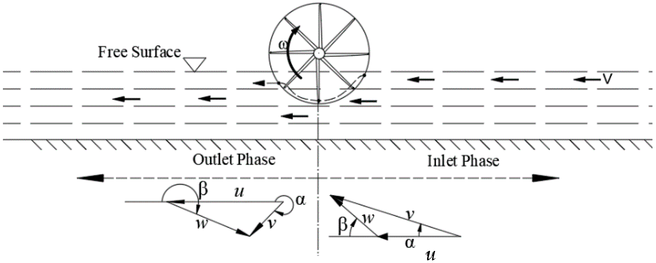
For boundary conditions, the velocity-inlet with an open channel and segregated velocity input was set to 0 m/s for the primary phase (air) and 3 m/s for the second phase (water). The free surface level is also set at the inlet in multiphase module. The free surface level and bottom level needed to be set for the pressure-outlet in the multiphase module. A low turbulent intensity of 1% was set for the pressure-outlet and velocity inlet [21]. The symmetry without a physical boundary was chosen for the top of the domain, considering the stability of the calculation. All other boundaries of the domain were used for the no-slip wall [21]. The immersed radius ratio is defined as , where the represents the immersed depth when the stream is not equipped with a wheel and is . In addition, the blockage ratio is used to specify the immersed radius ratio effect on the wheel’s performance [35,37]. The blockage ratio is defined as , where is the blade width (11 m), is the undisturbed flow depth (2.2 m) and is the channel width (11.4 m). The boundary condition and diagram of the water wheel operation are presented as Figure 3.
3. Reliability Verification
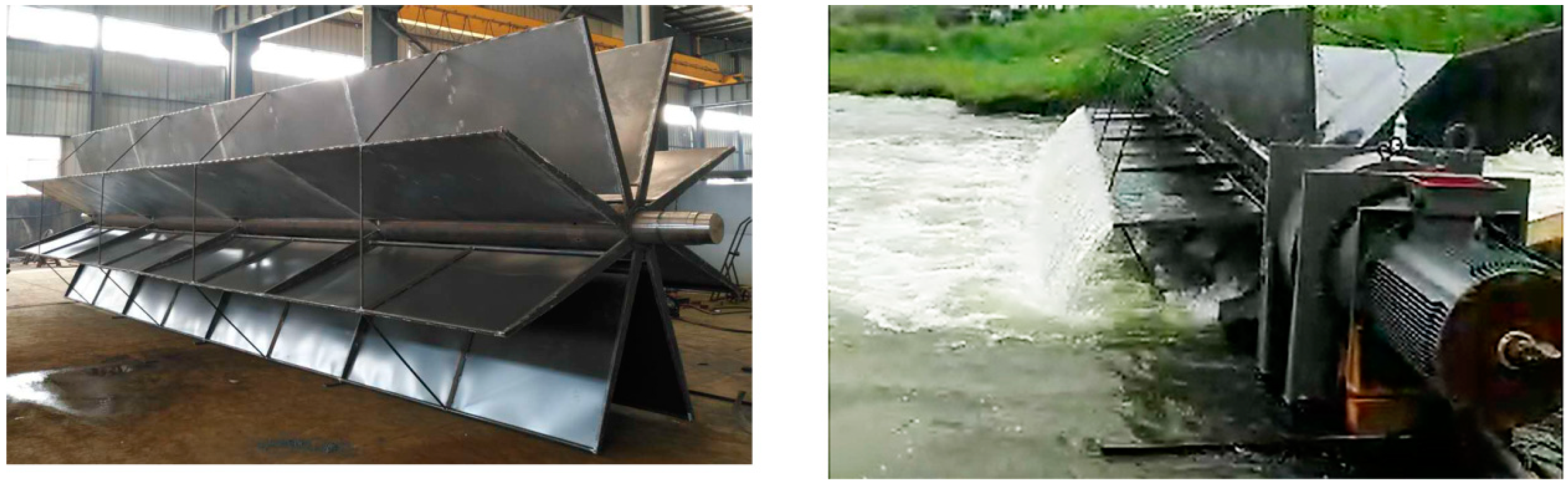
The case was experimented at an immersed depth of 0.8 m. The flow velocity at the inlet was measured by the Propeller Flow Velocity Meter (Jiangsu Nanshui Water Technology Co. Ltd., Nanjing, China) of LS1206B. It is mainly used to measure flow velocity in open channels. The main parameters of the instrument are as follow: the rotor diameter is 60 mm, the measured range of flow velocity is from 0.05 m/s to 7 m/s, relative error δ within ±5% and a staring speed of 0.05 m/s. For the accuracy of flow velocity, the flow velocity of 13 points located at the 11m in front of water wheel was measured. The average velocity of 13 points is regarded as the inlet-velocity in simulation. The GBM Power Station Control Center manufactured by GBM Co. Ltd. (Nanchang, China) is applied to measure the output and rotational speeds and it is manufactured by GBM Co. Ltd. The water wheel is connected with an axis of a permanent magnet generator through a gearbox with a transmission ratio of 1:25. The water wheel’s rational speeds can be converted from the rational speeds of the permanent magnet generator. The permanent magnet generator has a very high efficiency and the high torque was generated; the maximum error on the power measurement was estimated as no more than 2%. The GBM Power Station Control Center has two control models when making an automatic adaptation to the optimal speed and manual speed adjustment. In this experiment, the cases with optimum working condition and other different TSR were experimented at an immersed depth of 0.8 m. The test devices are shown in Figure 4. The field experiments are shown in Figure 5. The comparison of output between the experiments and numerical simulations is shown in Table 1.
The results of the simulation are consistent with the output of the experiments as a whole. The maximum error is relatively smaller, no more than 5%. The main reasons for the error are known as follow: Mechanical friction is seemed as the main source of the errors. There are also some differences with being a little wider downstream in the physical model than the actual channel; so, the diffusion may cause some hydraulic loss. In addition, the boundary conditions in the numerical simulation may cause some errors compared with actual flow.
4. Results and Discussion
4.1. Evaluation of Water Wheel Performance
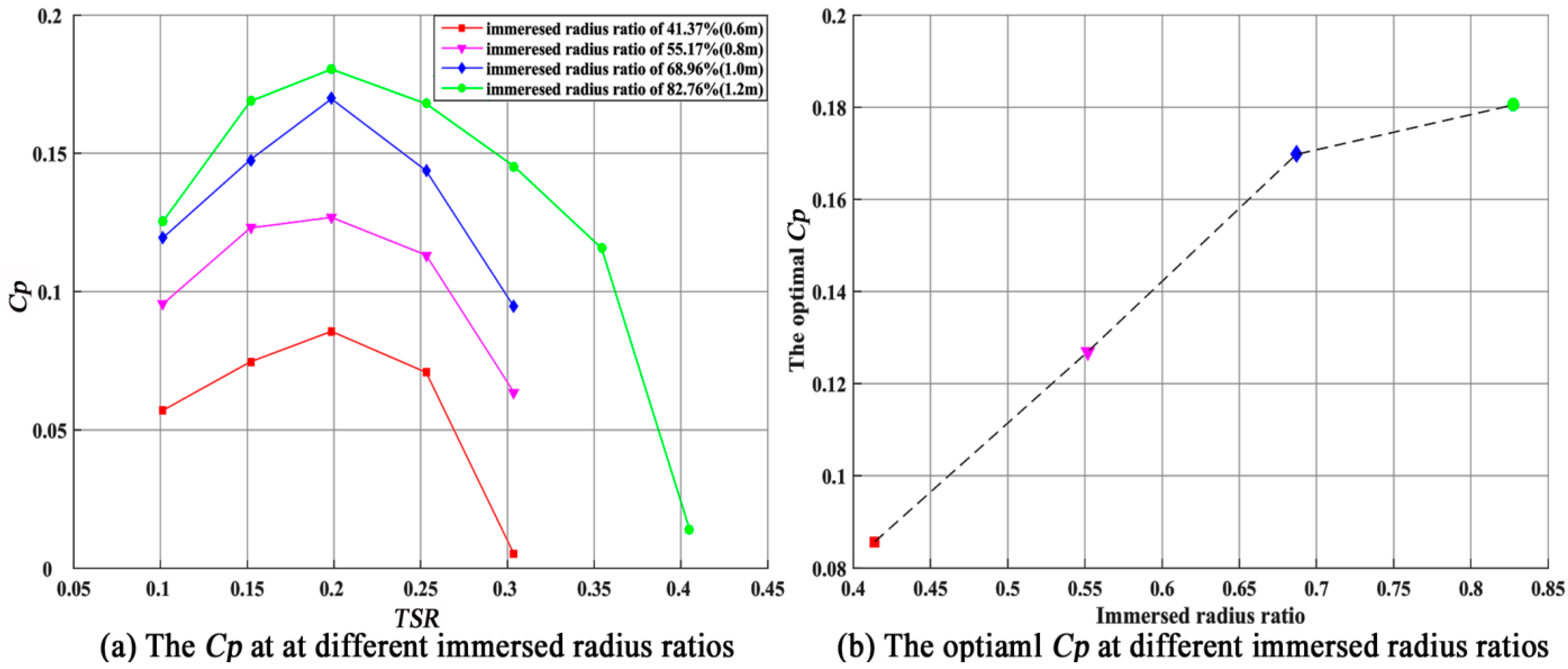
The different cases are researched at different immersed radius ratios. Table 2 indicates that the power coefficient is used at the immersed radius ratio of 41.37% (0.6 m) and 55.17% (0.8 m), and the efficiency is used at the immersed radius ratio of 41.37% (1.2 m). More specific, at the immersed radius ratio of 68.96% (1.0 m), the X is varied near 1 at different rotational speeds; this immersed radius ratio can be considered a transition from stream water wheel to RHPM, and here the power coefficient is used at this immersed radius ratio. The performance and optimal among the different immersed radius ratios are shown in Figure 6.
Figure 6 indicates that the different immersed ratios have a similar tendency to increase followed by decreasing at different cases. At different immersed depths, the range of increasing and decreasing is slightly different. At an immersed radius ratio 82.76% (1.2 m), the efficiency is increasing until TSR 0.1984, followed by decreasing until TSR 0.4049. At the other three cases, the efficiency performs the same tendency to increases followed by decreasing until TSR 0.3037. In summary, it can be said the operating range performs much wider at the immersed radius ratio of 82.76%; also, it has the same optimal rotational speeds at different cases. In addition, it can be found that the optimal is at a steady growth before the transition; however, after that, the optimal begins to increase at a lower rate until an immersed radius ratio of 82.76%.
At the immersed radius ratio of 82.76% (1.2 m), the maximum is 18.05% at a TSR of 0.1984, this is followed by 16.98% at an immersed radius ratio of 68.96% (1.0 m), 12.69% at an immersed radius ratio of 55.17% (0.8 m) and 8.57% at an immersed radius ratio of 41.37% (0.6 m) with an all TSR of 0.1984. Furthermore, the torque becomes negative at an immersed radius ratio of 96.56% (1.4 m), indicating that the water wheel cannot work at this working condition. The performance is much better as the immersed radius ratio increases for the stream wheel before an immersed radius ratio of 68.96% (1.0 m); after that, the water wheel at the immersed radius ratio of 82.76% (1.2 m) has the best performance in RHPM in all cases. Above all, it can be said that it shows much better performance at the immersed radius ratio of 82.76% (1.2 m) in all cases.
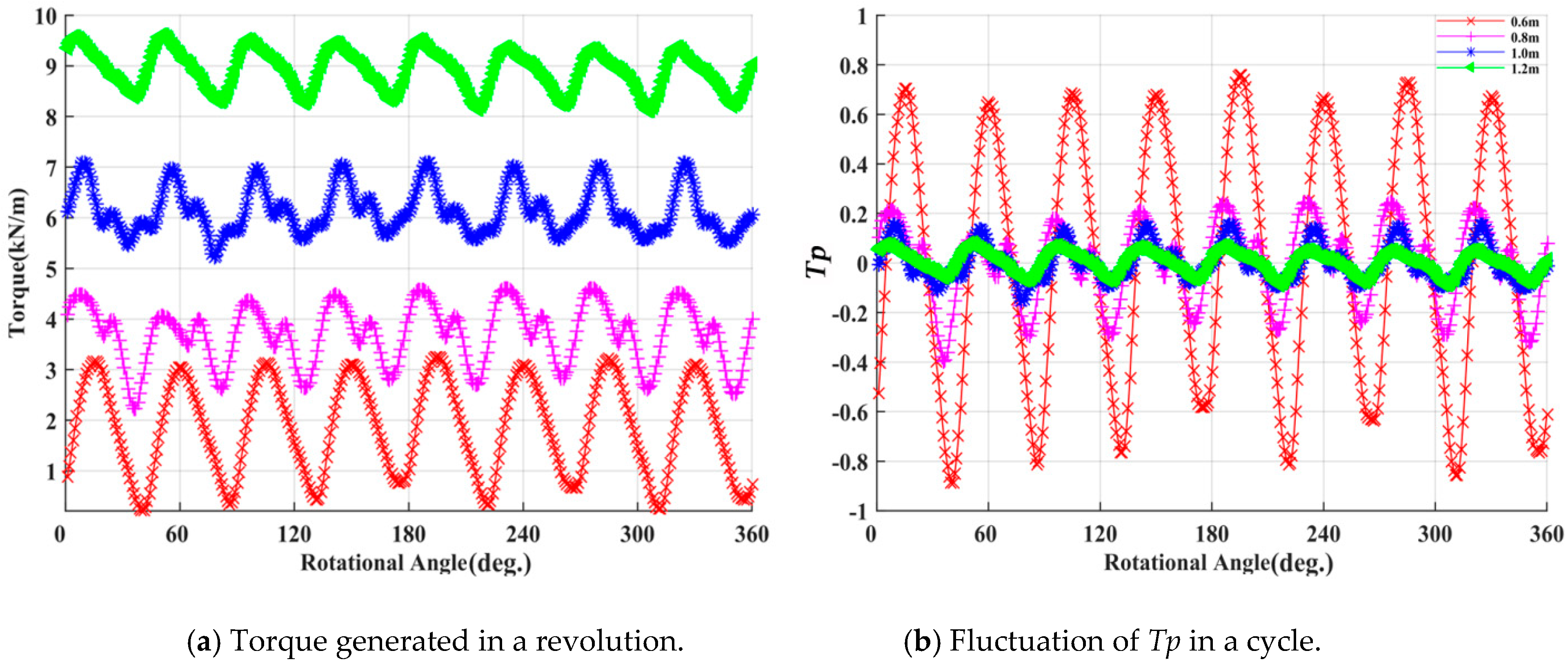
In order to describe the torque fluctuation, a non-dimensional parameter is defined, . is the torque at each time step. is a time-average torque. The computed torque is shown in Figure 7a in a revolution at a TSR of 0.1984 at different immersed depths; the is shown in Figure 7b. It is clear that the generated available torque fluctuated eight times in a cycle, and the angle for the period is . It can be said the period of fluctuation is consistent with the numbers of blades in a cycle. The available torque also dramatically increases at the beginning of a period, but the decrease in torque is much slower; the different cases present the same tendency in torque fluctuation. As discussed above, it generates much greater torques at the immersed depth of 1.2 m (immersed radius ratio of 82.76%). Moreover, the torque fluctuation is more stable at the immersed depth of 1.2 m than in other cases. Therefore, it can be said it can improve the performance and reduce the torque fluctuation by adding immersed depth until 1.2 m (immersed radius ratio of 82.76%).
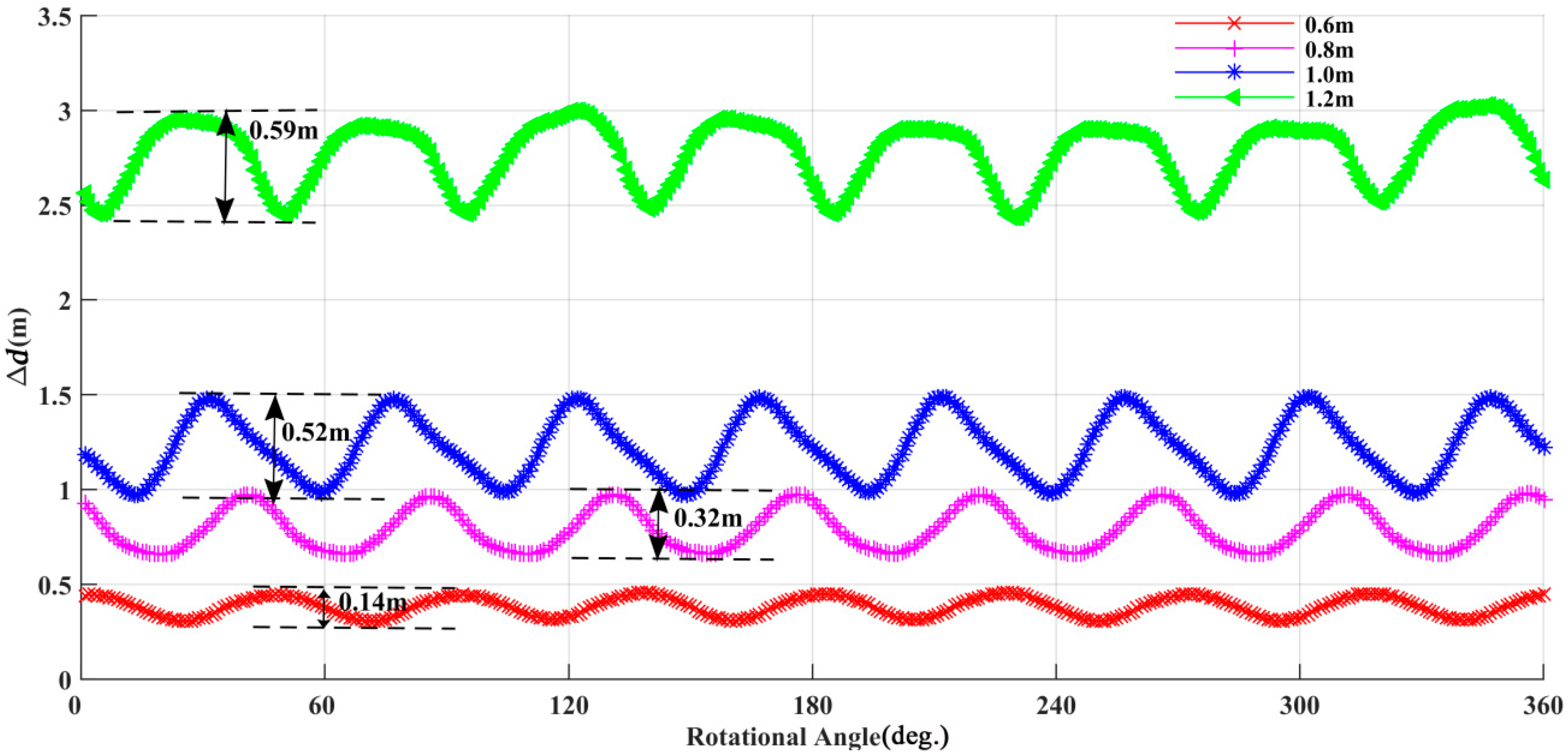
The computed difference in water level is presented in Figure 8 in a revolution at different immersed depths. The free surface is monitored at a TSR of 0.1984 from the center of the water wheel to a distance of 2D. It is clear that the average difference in water level increases as the immersed depth increases, also it drastically increases, and the maximum is nearly 3 m at the immersed depth of 1.2 m. The fluctuation of ∆d is much stronger than the other cases. So, it may cause the dramatic vibration and fatigue of the blades, which could pose a considerate threat to the security of the entire system. The high difference in water level may also cause serious erosion. Above all, it indicates that the fluctuation amplitude of the water level difference and the average water level difference increases as the immersed depth increases; also, the average water level difference is elevated considerably at the immersed depth of 1.2 m (immersed radius ratio of 82.76%). Furthermore, the water wheel gradually becomes a RHPM as the immersed depth increases [31]; the transition still needs to be researched.
4.2. Analysis of the Flow Fields and Velocity Triangles
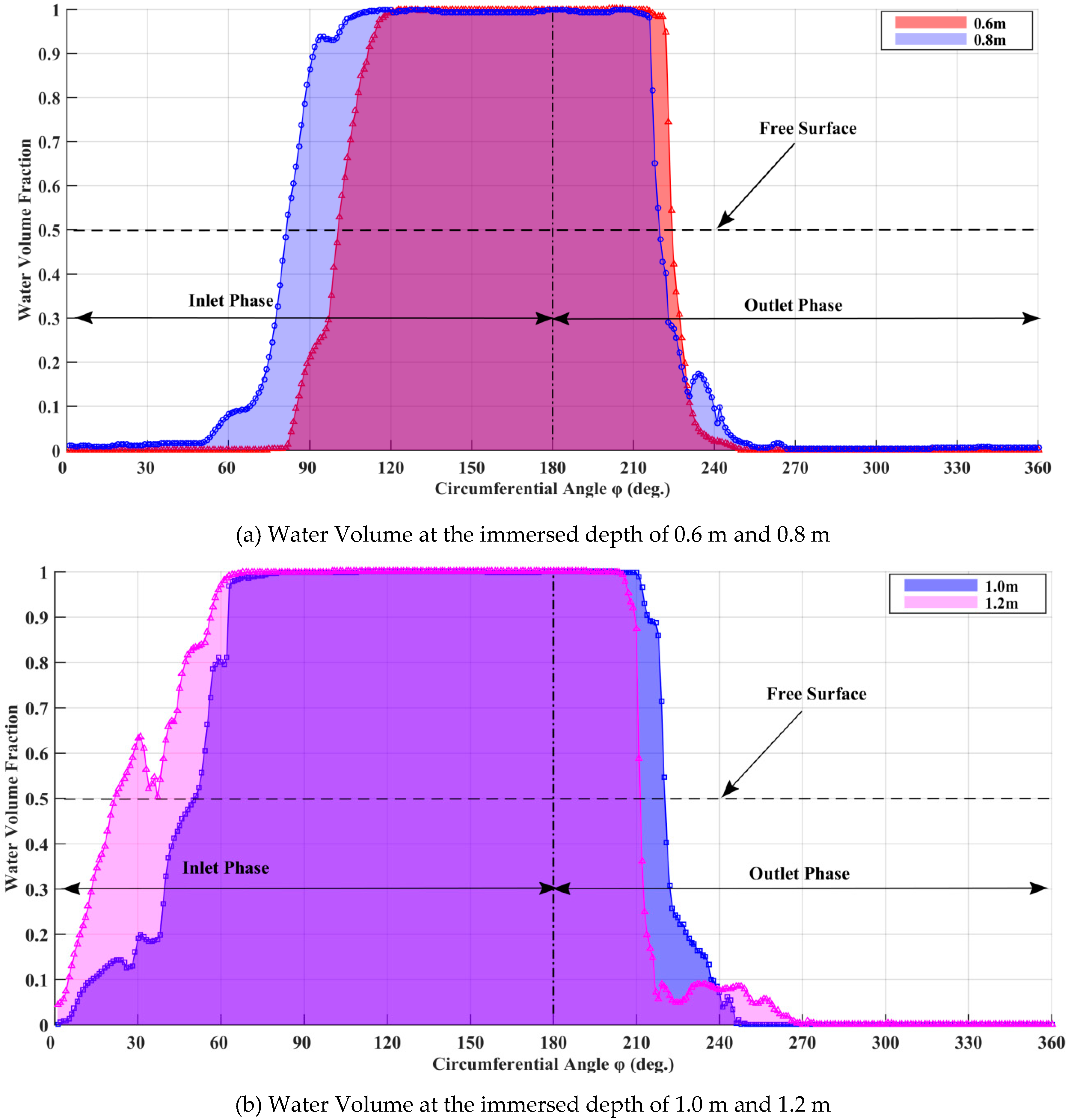
Flow characteristics are researched around the water wheel at different circumferential angle φ using numerical simulation, and they are considered as in the middle of the width of the water wheel. It is investigated at a TSR of 0.1984. The circumferential angle φ is expressed as a point at the top of the outside diameter of the wheel in the direction of the rotation. The comparison of water volume at different immersed depths is presented in Figure 9. The is known as the interface between water and air. is known as the water area, and air area is identified as . It is clear that it keeps the longest region of water area where some air is mixed with water at the immersed depth of 1.2 m. In contrast, water area at the immersed depth of 0.6 m has the shortest region at . Moreover, water area at the immersed depth of 1.0 m is slightly longer at than that of an immersed depth of 0.8 m at .
In addition, there are some significant differences from comparisons of the water volume fractions at the inlet phase. It is clearly seen that the water volume fraction at the inlet phase varies more strongly than the outlet phase as immersed depth increases, especially at an immersed depth of 1.0 m and 1.2 m; it indicates that much more air intrudes into the inlet stage as the blades are gradually submerged by the water. The water mixed with air may make the flow more complex at the inlet phase.
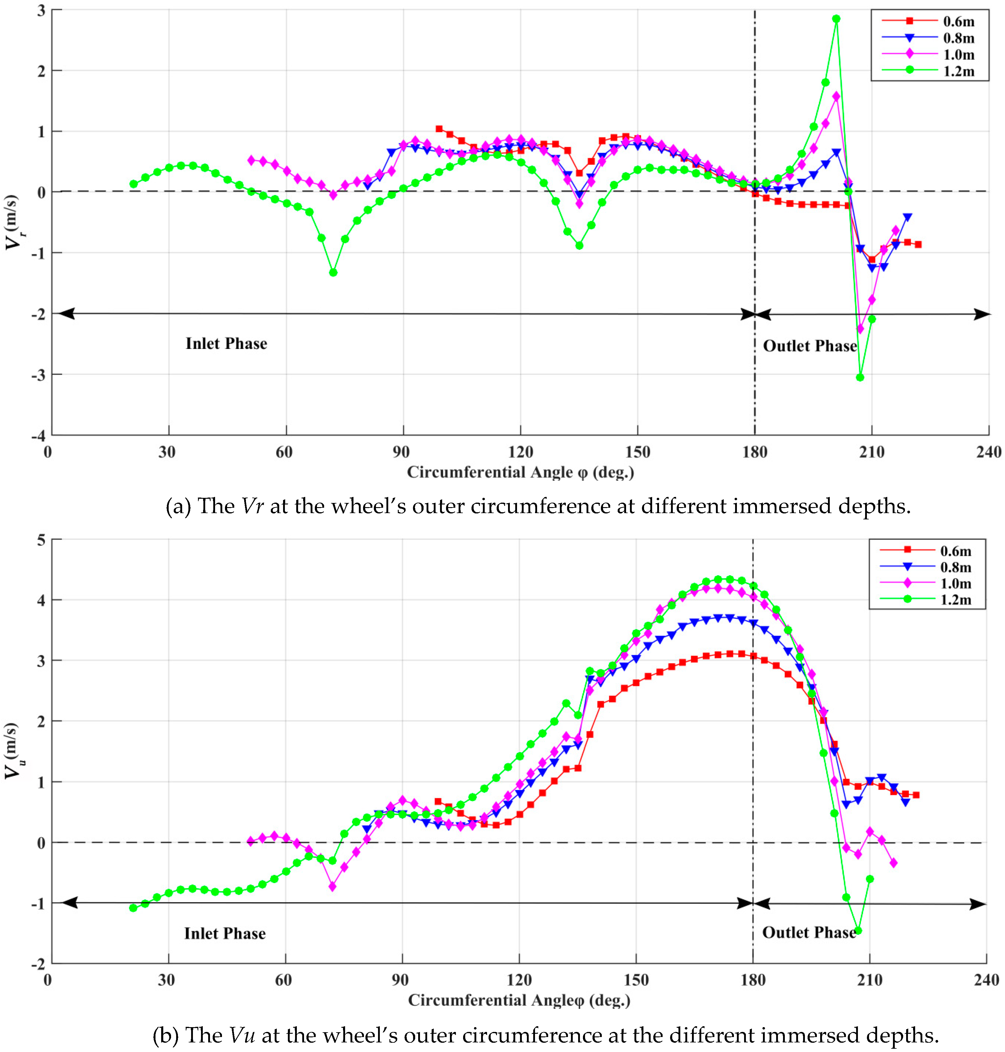
The diagram of velocity triangle is presented in Figure 10 at the inlet phase and the outlet phase. The absolute velocity has two components included, peripheral velocity (u) and relative velocity (w). The α is an absolute angle between peripheral velocity (u) and absolute velocity (v) and β is a relative angle between peripheral velocity (u) and relative velocity (w). The computed radial (Vr) and tangential (Vu) components of the absolute velocity (v) are used to make a comparison between the flow characteristics. The radial velocity (Vr) has a positive direction with a radial inner direction and tangential velocity (Vu) has a positive direction with a rotational direction. The Vr and Vu are identified in Figure 11 through the water volume fraction at different immersed depths and a TSR of 0.1984.
It can be seen that Vr shows a similar tendency at different immersed depths in a cycle from Figure 11a. The Vr decreases as increases from nearly ° to at different immersed depths. At the immersed depth of 1.2 m, the value of Vr performs much more negative and is relatively smaller at the inlet phase. It indicates the case at an immersed depth of 1.2 m and has the higher resistance for main flow. However, it can absorb more energy from water flow and has a better performance. After that, the values of Vr for all cases become positive and the water gradually flows into the flow channels between the blades, coupled at the beginning to generate a swirling flow. Then Vr gradually goes down and dramatically increases, arriving a peak nearly at . It can be referred that eddies begin to generate as water gathered in the flow channels between the blades at and it is fully developed at as Vr arrives at a peak. After that, the water in the flow channels between the blades quickly flows into the rivers with Vr achieving a minimum at nearly at the outlet phase, and the eddy fails to continue because of the loss of water and quickly disappears.
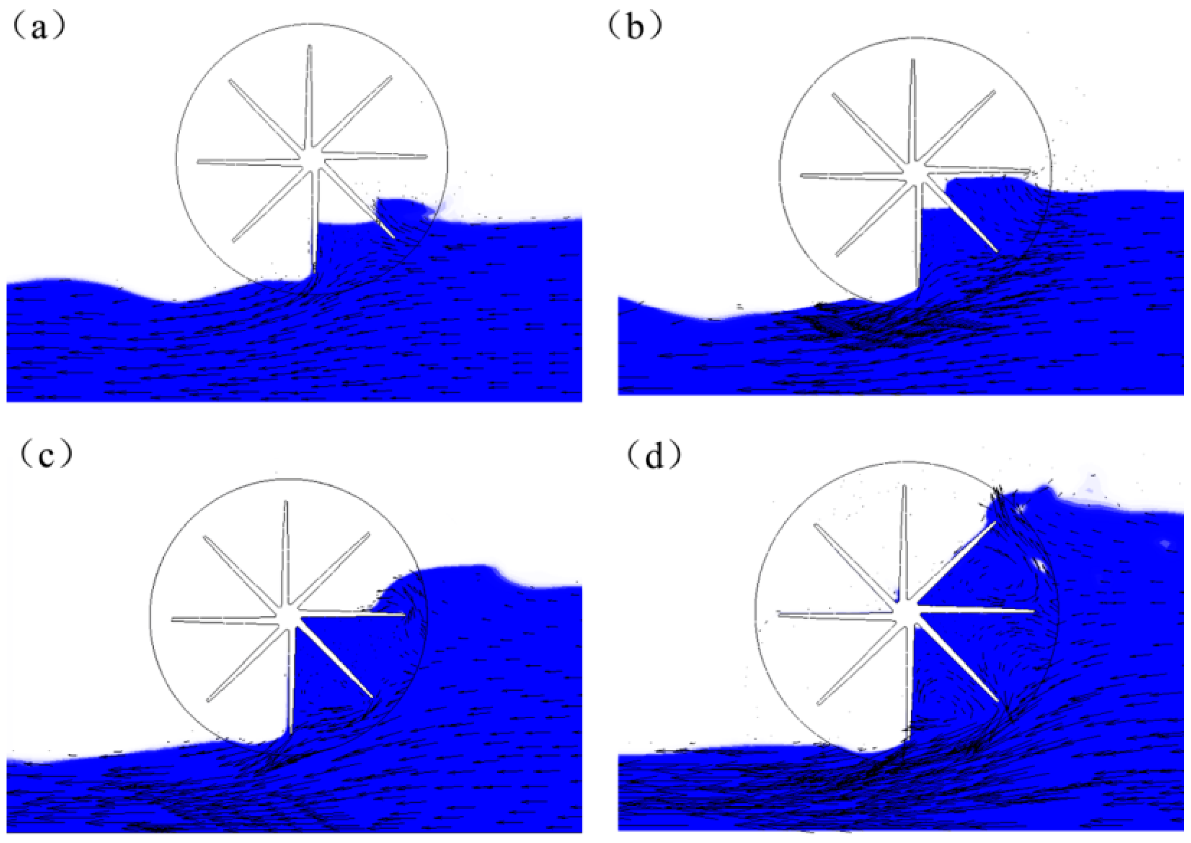
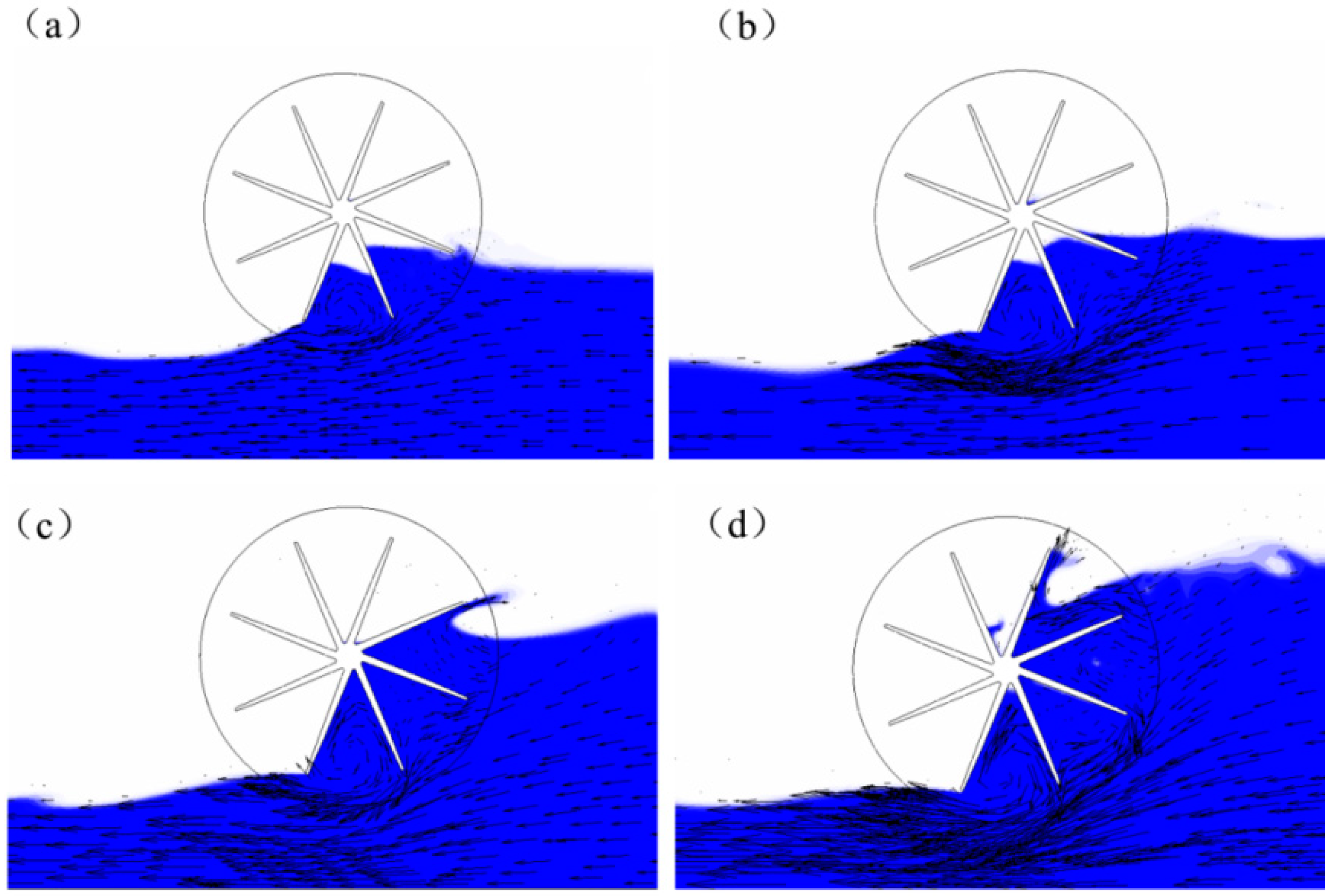
In addition, there are some differences at this area of : The water area is much larger because of the elevation at the upstream water level at the immersed depth of 1.2 m; also, the value of Vr varies strongly and dramatically decreases to negative coupled with achieving a minimum at , and then increases to positive. So, it can be inferred that it may cause more serious swirling flow between the different blades at this condition. The velocity vectors are presented in Figure 12 and Figure 13 at and , respectively. It can be seen that the eddy is gradually generated at and fully developed at in a flow channel expected of this case at the immersed depth of 1.2 m. At the immersed depth of 1.2 m, eddies generate in two flow channels and have developed an initial vortex at because of the elevation of the upstream water level. So, it can be said this case would cause more complex flow.
As shown in Figure 11b, tangential velocity (Vu) gradually increases at the inlet phase as the φ increases and achieves a peak nearly at at different immersed depths, also the value of gradually increases as the immersed depth increases at different cases. After that, Vu begins to decrease as the increases and the cases at a deep immersed depth have a faster rate of decline. Combined with the Vr at the outlet phase in Figure 11a, it can be said that the case at an immersed depth of 1.2 m performs a complex flow because of dramatic change in Vr and Vu. In summary, the flow would be more complex as the immersed depth increases and would cause serious local ersion coupled with eddies.
5. Conclusion and Future Work
The objective of this paper was to study the effect of different immersed depths on the performance and flow characteristics for a real-size water wheel applied in an open channel, and from the present research, the following conclusions can be made:
1. The results of the simulation are consistent with the output of the experiments as a whole. The simulations could represent the experiments with a maximum error of less than 5%.
2. The water wheel performance is much better as the immersed radius ratio increases of the stream wheel before an immersed radius ratio of 68.96% (1.0 m); after that, the water wheel at the immersed radius ratio of 82.76% (1.2 m) has the best performance as the RHPM in all cases. The case at an immersed radius ratio of 82.76% shows the best performance, achieving a maximum efficiency of 18.05% at a TSR of 0.1984. The maximum efficiency is followed by 16.98% at an immersed radius ratio of 68.96%, 12.69% at an immersed radius ratio of 55.17% and 8.6% at an immersed radius ratio of 41.37%, with all TSR = 0.1984. It suggests the immersed depth at an immersed radius ratio of 82.76% can be applied for a much better performance.
3. The case at the immersed radius ratio of 82.76% has a wider operating range and it can work at high speeds or low torque; the optimal speed is at different cases. The torque is more stable as the immersed radius ratio increases less than 82.76%. The wheel mainly work at a low TSR, that is a ; also, the wheel has a higher efficiency at (the TSR is equal to ) as in Reference [31], and thus it can be said the results is consistent with each other.
4. The average water-level difference between the upstream and downstream areas increases as the immersed radius ratio increases less than 82.76%. The average water-level difference is dramatically elevated at the immersed radius ratio of 82.76% (1.2 m); it has a greater average water level difference and fluctuation amplitude than other cases. In addition, the case at the immersed radius ratio of 68.96% is a transition from stream wheel to RHPM; the optimal steadily increases before transition, however, after that, the optimal begins to increase much more slowly until an immersed radius ratio of 82.76%. Furthermore, the transition still needs much more research.
5. The water region is much wider and the water volume fraction shows more intense changes at the inlet stage than the outlet phase as the immersed depth increases. In addition, at the immersed radius ratio of 82.76% (1.2 m), much more air intrudes into the water between the blades at the inlet stage and, coupled with the dramatic change in water volume fraction, would make flow more complex.
6. An eddy was gradually generated and fully developed in the single flow channel at the same time except at the immersed radius ratio of 82.76% (1.2 m). At the immersed radius ratio of 82.76% (1.2 m), eddies generated in two flow channels and can develop an initial vortex earlier than other cases because of the elevation of the upstream water level. Combined with dramatic changes in Vr and Vu, flow would be more complex as the immersed depth increases and may cause serious local ersion coupled with swirling flow.
Author Contributions
Conceptualization, C.Y.; formal analysis, M.Z.; funding acquisition, C.Y. and Y.Z.; investigation, C.Y.; methodology, Q.T.; resources, Y.Z; software, Y.Z; supervision, C.Y.; validation, M.Z. and C.Y.; writing—original draft, M.Z. and C.Y.; writing—review and editing, C.Y. and Y.Z. All authors have read and agreed to the published version of the manuscript.
Funding
This research was funded by the National Natural Science Foundation of China (51709086), National Natural Science Foundation of China (No. 51809083), Natural Science Foundation of Jiangsu Province (No. BK20180504).
Acknowledgments
The authors are grateful for support from GBM Co. Ltd. and College of Water Conservancy and Hydropower Engineering, Hohai University.
Conflicts of Interest
The authors declare no conflict of interest.
Nomenclature
| λ | Tip-speed ratio |
| Ratio of the energy extraction by water wheel to energy available in the water | |
| Values between the upstream and downstream water depths | |
| Fluctuation amplitude ratio of water level | |
| Water density | |
| Water volume fractions | |
| The angle of a point at the top of the outside diameter of wheel in direction of rotation | |
| Vu | Tangential components of the absolute velocity |
| Vr | Radial components of the absolute velocity |
References
- Jones, Z. Domestic Electricity Generation Using Waterwheels on Moored Barge. Master’s Thesis, School of theBuilt Ennvironment, Heriot-Watt University, Edinburgh, UK, 2005. [Google Scholar]
- Choi, Y.; Yoon, H.; Inagaki, M.; Ooike, S.; Kim, Y.J.; Lee, Y.H. Performance improvement of a cross-flow hydro turbine by air layer effect. In IOP Conference Series: Earth and Environmental Science; IOP Publishing: Bristol, UK, 2010; p. 012030. [Google Scholar]
- Choi, Y.-D.; Lim, J.-I.; Kim, Y.-T.; Lee, Y.H. Performance and internal flow characteristics of a cross-flow hydro turbine by the shapes of nozzle and runner blade. J. Fluid Sci. Technol. 2008, 3, 398–409. [Google Scholar] [CrossRef] [Green Version]
- Bartle, A. Hydropower potential and development activities. Energy Policy 2002, 30, 1231–1239. [Google Scholar] [CrossRef]
- Zapata, S.; Castaneda, M.; Aristizabal, A.J.; Cherni, J.; Dyner, I. Assessing renewable energy policy integration cost, emissions and affordability the Argentine case. In Proceedings of the Decarbonization, Efficiency and Affordability: New Energy Markets in Latin America, 7th ELAEE/IAEE Latin American Conference, Buenos Aires, Argentina, 10–12 March 2019. [Google Scholar]
- Senior, J.; Wiemann, P.; Muller, G. The rotary hydraulic pressure machine for very low head hydropower sites. In Proceedings of the Hidroenergia Conference, Wroclaw, Poland, 23–26 May 2008; pp. 1–8. [Google Scholar]
- Murdock, H.E.; Gibb, D.; André, T.; Appavou, F.; Brown, A.; Epp, B.; Kondev, B.; McCrone, A.; Musolino, E.; Ranalder, L.; et al. Renewables 2019 Global Status Report. 2019. Available online: https://wedocs.unep.org/handle/20.500.11822/28496 (accessed on 22 December 2019).
- Pujol, T.; Montoro, L. High hydraulic performance in horizontal waterwheels. Renew. Energy 2010, 35, 2543–2551. [Google Scholar] [CrossRef]
- Müller, G.; Kauppert, K. Performance characteristics of water wheels. J. Hydraul. Res. 2004, 42, 451–460. [Google Scholar] [CrossRef]
- Turnock, S.R.; Muller, G.; Nicholls-Lee, R.F.; Denchfield, S.; Hindley, S.; Shelmerdine, R.; Stevens, S. Development of a floating tidal energy system suitable for use in shallow water. 2007. Available online: https://eprints.soton.ac.uk/48752/1/1055.pdf (accessed on 19 January 2020).
- Quaranta, E. Investigation and Optimization of the Performance of Gravity Water Wheels. Ph.D. Thesis, Politecnico di Torino, Torino, Italy, 2017. under review. [Google Scholar]
- Quaranta, E.; Revelli, R. Optimization of breastshot water wheels performance using different inflow configurations. Renew. Energy 2016, 97, 243–251. [Google Scholar] [CrossRef]
- Quaranta, E.; Revelli, R. Output power and power losses estimation for an overshot water wheel. Renew. Energy 2015, 83, 979–987. [Google Scholar] [CrossRef]
- Quaranta, E.; Revelli, R. Performance characteristics, power losses and mechanical power estimation for a breastshot water wheel. Energy 2015, 87, 315–325. [Google Scholar] [CrossRef]
- Quaranta, E.; Müller, G. Sagebien and Zuppinger water wheels for very low head hydropower applications. J. Hydraul. Res. 2018, 56, 526–536. [Google Scholar] [CrossRef] [Green Version]
- Quaranta, E.; Revelli, R. CFD simulations to optimize the blade design of water wheels. Drink. Water Eng. Sci. 2017, 10, 27–32. [Google Scholar] [CrossRef] [Green Version]
- Quaranta, E.; Revelli, R. Hydraulic behavior and performance of breastshot water wheels for different numbers of blades. J. Hydraul. Eng. ASCE 2016, 143, 04016072. [Google Scholar] [CrossRef]
- Jasa, L.; Priyadi, A.; Purnomo, M.H. Experimental Investigation of Micro-Hydro Waterwheel Models to Determine Optimal Efficiency. Appl. Mech. Mater. 2015, 776, 413–418. [Google Scholar] [CrossRef]
- Nishi, Y.; Inagaki, T.; Li, Y.; Omiya, R.; Fukutomi, J. Study on an undershot cross-flow water turbine. J. Therm. Sci. 2014, 23, 239–245. [Google Scholar] [CrossRef]
- Nguyen, M.H.; Jeong, H.; Jhang, S.S.; Kim, B.G.; Yang, C. A parametric study about blade shapes and blade numbers of water wheel type tidal turbine by numerical method. J. Korean Soc. Mar. Environ. Saf. 2016, 22, 296–303. [Google Scholar] [CrossRef]
- Nguyen, M.H.; Jeong, H.; Yang, C. A study on flow fields and performance of water wheel turbine using experimental and numerical analyses. Sci. China Technol. Sci. 2018, 61, 464–474. [Google Scholar] [CrossRef]
- Adanta, D.; Arifianto, S.A.; Nasution, S.B. Effect of Blades Number on Undershot Waterwheel Performance with Variable Inlet Velocity. In Proceedings of the 2018 4th International Conference on Science and Technology (ICST), Yogyakarta, Indonesia, 7–8 August 2018; pp. 1–6. [Google Scholar]
- Nishi, Y.; Inagaki, T.; Li, Y.; Omiya, R.; Hatano, K. Research on the flow field of undershot cross-flow water turbines using experiments and numerical analysis. In Proceedings of the IOP Conference Series: Earth and Environmental Science, Jakarta, Indonesia, 23–24 January 2014; p. 062006. [Google Scholar]
- Tevata, A.; Inprasit, C. The effect of paddle number and immersed radius ratio on water wheel performance. Energy Procedia 2011, 9, 359–365. [Google Scholar] [CrossRef] [Green Version]
- Castro-García, M.; Rojas-Sola, J.I. Technical and functional analysis of Albolafia waterwheel (Cordoba, Spain): 3D modeling, computational-fluid dynamics simulation and finite-element analysis. Energy Conv. Manag. 2015, 92, 207–214. [Google Scholar] [CrossRef]
- Vidali, C.; Fontan, S.; Quaranta, E.; Cavagnero, P.; Revelli, R. Experimental and dimensional analysis of a breastshot water wheel. J. Hydraul. Res. 2016, 54, 473–479. [Google Scholar] [CrossRef]
- Nguyen, M.H.; Kim, J.H.; Kim, B.K.; Yang, C. A Comparison of Performance of Six and Twelve-Blade Vane Tidal Turbines between Single and Double Blade-row Types. Korean Soc. Fluid Mech. 2015, 18, 51–58. [Google Scholar]
- Muller, G. The effect of using upper shroud on the performance of a breashoot water wheel. J. Phys. Conf. Ser. 2019, 012269. [Google Scholar]
- Masud, I.; Yusuke, S.; Suwa, Y. Performance prediction of zero head turbine at different water levels. In Proceedings of the IOP Conference Series: Earth and Environmental Science, Bogor, Indonesia, 10–11 September 2019; p. 012048. [Google Scholar]
- Paudel, S.; Linton, N.; Zanke, U.C.; Saenger, N. Experimental investigation on the effect of channel width on flexible rubber blade water wheel performance. Renew. Energy 2013, 52, 1–7. [Google Scholar] [CrossRef]
- Butera, I.; Fontan, S.; Poggi, D.; Quaranta, E.; Revelli, R. Experimental Analysis of Effect of Canal Geometry and Water Levels on Rotary Hydrostatic Pressure Machine. J. Hydraul. Eng. ASCE 2020, 146, 04019071. [Google Scholar] [CrossRef]
- Cleynen, O.; Kerikous, E.; Hoerner, S.; Thévenin, D. Characterization of the performance of a free-stream water wheel using computational fluid dynamics. Energy 2018, 165, 1392–1400. [Google Scholar] [CrossRef]
- Batten, W.M.J.; Weichbrodt, F.; Muller, G.U.; Hadler, J.; Semlow, C.; Hochbaum, M.; Dimke, S.; Frohle, P. Design and stability of a floating free stream energy converter. In Proceedings of the 34th World Congress of the International Association for Hydro-Environment Research and Engineering: 33rd Hydrology and Water Resources Symposium and 10th Conference on Hydraulics in Water Engineering, Brisbane, Australia, 26 June–1 July 2011; p. 2372. [Google Scholar]
- Wulandari, R.; Mizar, M.A.; Andoko. Optimization design of Goose-Leg waterwheel next-G to extract energy of free water flow. AIP Conf. Proc. 2016, 030068. [Google Scholar]
- Müller, G.; Jenkins, R.; Batten, W. Potential, performance limits and environmental effects of floating water mills. River Flow 2010, 2010, 707–712. [Google Scholar]
- Muller, G.; Denchfield, S.; Marth, R.; Shelmerdine, B. Stream wheels for applications in shallow and deep water. In Proceedings of the Congress-International Association for Hydraulic Research, Venice, Italy, 1–6 July 2007; p. 707. [Google Scholar]
- Quaranta, E. Stream water wheels as renewable energy supply in flowing water: Theoretical considerations, performance assessment and design recommendations. Energy Sustain. Dev. 2018, 45, 96–109. [Google Scholar] [CrossRef]
- Kumar, A.; Saini, R. Performance analysis of a Savonius hydrokinetic turbine having twisted blades. Renew. Energy 2017, 108, 502–522. [Google Scholar]
- Nakajima, M.; Iio, S.; Ikeda, T. Performance of Savonius rotor for environmentally friendly hydraulic turbine. J. Fluid Sci. Technol. 2008, 3, 420–429. [Google Scholar] [CrossRef] [Green Version]
- Sule, L.; Rompas, P. Performance of Savonius Blade Waterwheel with Variation of Blade Number. In Proceedings of the IOP Conference Series: Materials Science and Engineering, Nanjing, China, 17–19 August 2018; p. 012073. [Google Scholar]
- Yaakob, O.; Ismail, M.A.; Ahmed, Y.M. Parametric Study for Savonius Vertical Axis Marine Current Turbine using CFD Simulation. In Proceedings of the 7th International Conference on Renewable Energy Sources (RES’13), Kuala Lumpur, Malaysia, 2–4 April 2013; pp. 200–205. [Google Scholar]
- Golecha, K.; Eldho, T.; Prabhu, S. Influence of the deflector plate on the performance of modified Savonius water turbine. Appl. Energy 2011, 88, 3207–3217. [Google Scholar] [CrossRef]
- Hassanzadeh, A.R.; Ahmed, Y.M.; Ismail1c, M.A. Numerical simulation for unsteady flow over marine current turbine rotors. Wind Struct. 2016, 23, 301–311. [Google Scholar] [CrossRef]
- Adanta, D.; Budiarso, W.; Siswantara, A.I. Assessment of turbulence modelling for numerical simulations into pico hydro turbine. J. Adv. Res. Fluid Mech. Therm. Sci. 2018, 46, 21–31. [Google Scholar]
- Kodirov, D.; Tursunov, O. Calculation of Water Wheel Design Parameters for Micro Hydroelectric Power Station. E3S Web Conf. 2019, 97, 05042. [Google Scholar] [CrossRef]
- Akinyemi, O.S.; Liu, Y. CFD modeling and simulation of a hydropower system in generating clean electricity from water flow. Int. J. Energy Environ. Eng. 2015, 6, 357–366. [Google Scholar] [CrossRef] [Green Version]
- Zaman, A.; Khan, T. Design of a water wheel for a low head micro hydropower system. J. Basic Sci. Technol. 2012, 1, 1–6. [Google Scholar]
- Akinyemi, O.S.; Chambers, T.L.; Liu, Y. Evaluation of the power generation capacity of hydrokinetic generator device using computational analysis and hydrodynamic similitude. J. Power Energy Eng. 2015, 3, 71. [Google Scholar] [CrossRef] [Green Version]
- Senior, J.A. Hydrostatic Pressure Converters for the Exploitation of Very Low Head Hydropower Potential. Ph.D. Thesis, University of Southampton, Southampton, UK, 2009. [Google Scholar]
- Denny, M. The efficiency of overshot and undershot waterwheels. Eur. J. Phys. 2003, 25, 193. [Google Scholar] [CrossRef] [Green Version]
- Al Sam, A. Water Wheel CFD Simulations. 2010. Available online: http://lup.lub.lu.se/student-papers/record/1698088 (accessed on 22 December 2019).
- Nasir Mehmood, Z.L.; Khan, J. Diffuser augmented horizontal axis tidal current turbines. Res. J. Appl. Sci. Eng. Technol. 2012, 4, 3522–3532. [Google Scholar]
- Acharya, N.; Kim, C.G.; Thapa, B.; Lee, Y.H. Numerical analysis and performance enhancement of a cross-flow hydro turbine. Renew. Energy 2015, 80, 819–826. [Google Scholar] [CrossRef]
- Zhang, Y.; Li, C.; Xu, Y.; Tang, Q.; Zheng, Y.; Liu, H.; Fernandez-Rodriguez, E. Study on Propellers Distribution and Flow Field in the Oxidation Ditch Based on Two-Phase CFD Model. Water 2019, 11, 2506. [Google Scholar] [CrossRef] [Green Version]
- Zhang, Y.; Xu, Y.; Zheng, Y.; Fernandez-Rodriguez, E.; Sun, A.; Yang, C.; Wang, J. Multiobjective Optimization Design and Experimental Investigation on the Axial Flow Pump with Orthogonal Test Approach. Complexity 2019, 2019. [Google Scholar] [CrossRef] [Green Version]
Figure 1.
Geometric model and grids of the wheel domain.

Figure 2.
Mesh dependence test.

Figure 3.
Boundary condition and diagram of water wheel operation.

Figure 4.
Test devices.

Figure 5.
Model of the water wheel and field experiment.

Figure 6.
The and optimal among different immersed radius ratios.

Figure 7.
Torque variation in a cycle.

Figure 8.
between the upstream and downstream in a cycle (m).

Figure 9.
Water volume of different immersed depths at the wheel’s outer circumference.

Figure 10.
Diagram of velocity triangles.

Figure 11.
Comparison of Vr and Vu at the wheel’s outer circumference.

Figure 12.
Velocity vectors at circumferential angle . (a) The immersed depth of 0.6 m; (b) the immersed depth of 0.8 m; (c) the immersed depth of 1.0 m; (d) the immersed depth of 1.2 m.
Figure 12.
Velocity vectors at circumferential angle . (a) The immersed depth of 0.6 m; (b) the immersed depth of 0.8 m; (c) the immersed depth of 1.0 m; (d) the immersed depth of 1.2 m.

Figure 13.
Velocity vectors at circumferential angle . (a) The immersed depth of 0.6 m; (b) the immersed depth of 0.8 m; (c) the immersed depth of 1.0 m; (d) the immersed depth of 1.2 m.
Figure 13.
Velocity vectors at circumferential angle . (a) The immersed depth of 0.6 m; (b) the immersed depth of 0.8 m; (c) the immersed depth of 1.0 m; (d) the immersed depth of 1.2 m.


Table 1.
Output of experiment and numerical simulation at an immersed depth of 0.8 m.
| Inlet Velocity (m/s) | Numbers of Blade | Rotational Speeds (r/min) | Output in Experiments (kW) | Output in Numerical Simulation (kW) | Error (%) |
|---|---|---|---|---|---|
| 3.0 | 8 | 2 | 10.90 | 11.34 | 4.1 |
| 3 | 14.09 | 14.61 | 3.7 | ||
| 3.92 (Optimal speeds) | 14.52 | 15.07 | 3.6 | ||
| 5 | 9.66 | 10.12 | 4.7 | ||
| 6 | 5.43 | 5.62 | 3.4 |
Table 2.
The main characteristic parameters.
| Immersed Depth (m) | Immersed Radius Ratio | Blockage Ratio | X |
|---|---|---|---|
| 0.6 | |||
| 0.8 | |||
| 1.0 | |||
| 1.2 |
© 2020 by the authors. Licensee MDPI, Basel, Switzerland. This article is an open access article distributed under the terms and conditions of the Creative Commons Attribution (CC BY) license (http://creativecommons.org/licenses/by/4.0/).
Share and Cite
MDPI and ACS Style
Zhao, M.; Zheng, Y.; Yang, C.; Zhang, Y.; Tang, Q. Performance Investigation of the Immersed Depth Effects on a Water Wheel Using Experimental and Numerical Analyses. Water 2020, 12, 982. https://doi.org/10.3390/w12040982
AMA Style
Zhao M, Zheng Y, Yang C, Zhang Y, Tang Q. Performance Investigation of the Immersed Depth Effects on a Water Wheel Using Experimental and Numerical Analyses. Water. 2020; 12(4):982. https://doi.org/10.3390/w12040982
Chicago/Turabian StyleZhao, Mengshang, Yuan Zheng, Chunxia Yang, Yuquan Zhang, and Qinghong Tang. 2020. "Performance Investigation of the Immersed Depth Effects on a Water Wheel Using Experimental and Numerical Analyses" Water 12, no. 4: 982. https://doi.org/10.3390/w12040982
Note that from the first issue of 2016, this journal uses article numbers instead of page numbers. See further details here.