Benefits of Combining Satellite-Derived Snow Cover Data and Discharge Data to Calibrate a Glaciated Catchment in Sub-Arctic Iceland


 ,
, 
Abstract
:1. Introduction
1.1. Background
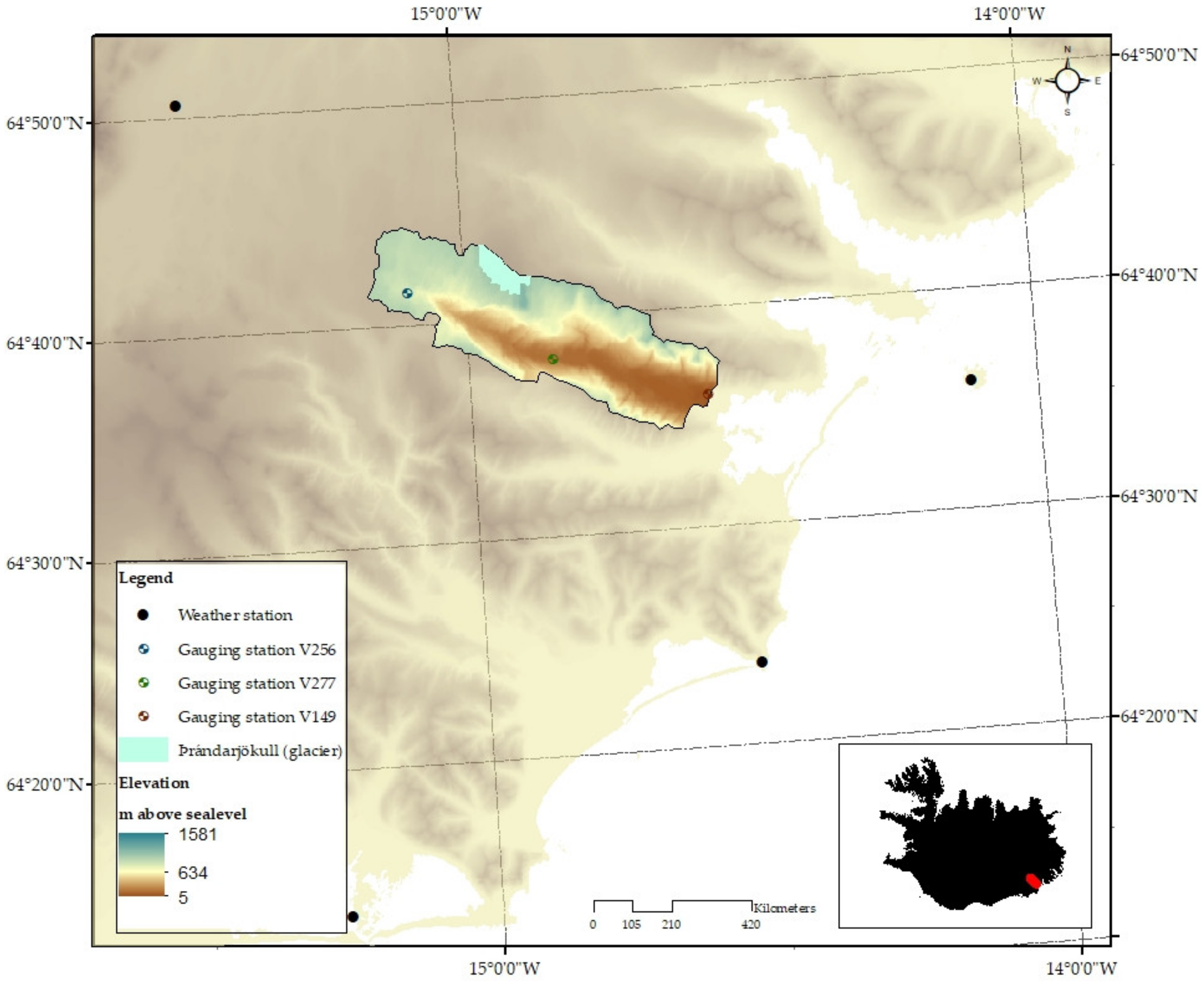
1.2. Study Area
2. Materials and Methods
2.1. Input Data and Calibration Data
2.2. Model Description
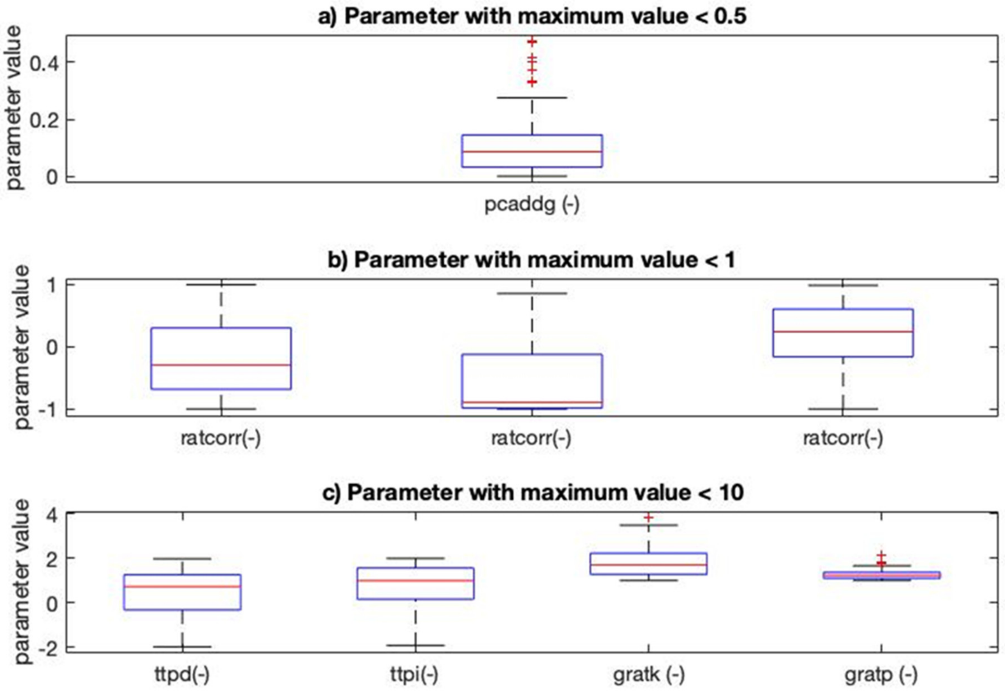
2.3. Parameter Selection and Calibration
2.4. Performance Criteria
2.5. Calibration Using SDC and MDC
3. Results
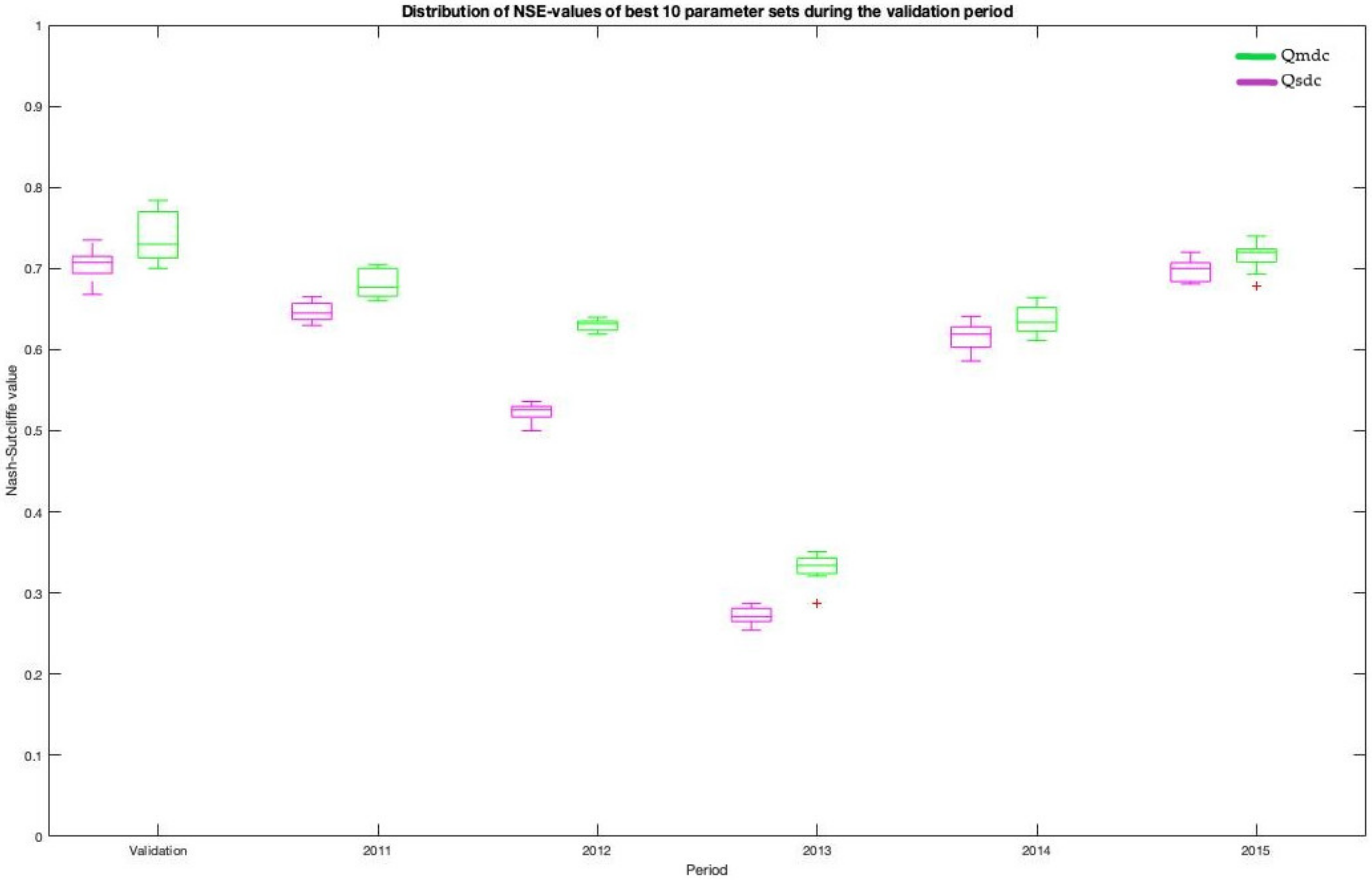
3.1. Overall Performance
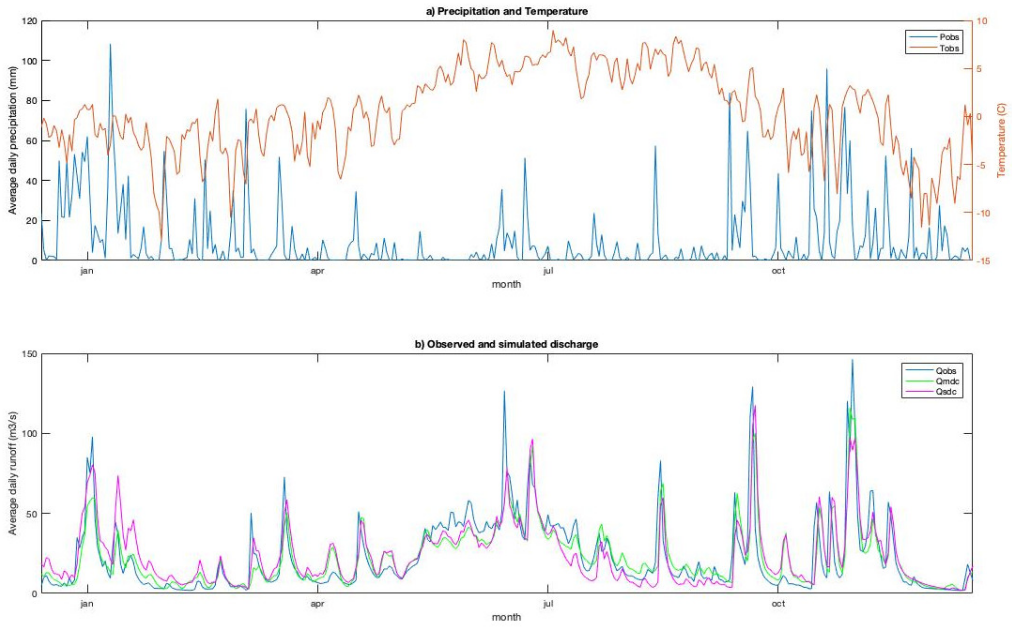
3.2. Discharge Simulations
3.3. Fractional Snow Cover Area Simulations
4. Discussion
Uncertainty, Limitations, and Future Research
5. Conclusions
Author Contributions
Funding
Acknowledgments
Conflicts of Interest
Data Availability
Appendix A


References
- Juston, J.; Seibert, J.; Johansson, P.O. Temporal sampling strategies and uncertainty in calibrating a conceptual hydrological model for a small boreal catchment. Hydrol. Process. 2009, 23, 3093–3109. [Google Scholar] [CrossRef]
- Kalantari, Z.; Briel, A.; Lyon, S.W.; Olofsson, B.; Folkeson, L. On the utilization of hydrological modelling for road drainage design under climate and land use change. Sci. Total. Environ. 2014, 475, 97–103. [Google Scholar] [CrossRef]
- Hannah, D.M.; Kansakar, S.R.; Gerrard, A.J.; Rees, G. Flow regimes of Himalayan rivers of Nepal: Nature and spatial patterns. J. Hydrol. 2005, 308, 18–32. [Google Scholar] [CrossRef]
- Nijssen, B.; O’donnell, G.M.; Hamlet, A.F.; Lettenmaier, D.P. Hydrologic sensitivity of global rivers to climate change. Clim. Chang. 2001, 50, 143–175. [Google Scholar] [CrossRef]
- Reedyk, S.; Woo, M.K.; Prowse, T.D. Contribution of icing ablation to streamflow in a discontinuous permafrost area. Can. J. Earth Sci. 1995, 32, 13–20. [Google Scholar] [CrossRef]
- Refsgaard, J.C.; Knudsen, J. Operational validation and intercomparison of different types of hydrological models. Water Resour. Res. 1996, 32, 2189–2202. [Google Scholar] [CrossRef]
- Sorooshian, S.; Gupta, V.K.; Fulton, J.L. Evaluation of maximum likelihood parameter estimation techniques for conceptual rainfall-runoff models: Influence of calibration data variability and length on model credibility. Water Resour. Res. 1983, 19, 251–259. [Google Scholar] [CrossRef]
- Yapo, P.O.; Gupta, H.V.; Sorooshian, S. Automatic calibration of conceptual rainfall-runoff models: Sensitivity to calibration data. J. Hydrol. 1996, 181, 23–48. [Google Scholar] [CrossRef]
- Anctil, F.; Perrin, C.; Andréassian, V. Impact of the length of observed records on the performance of ANN and of conceptual parsimonious rainfall-runoff forecasting models. Environ. Model. Softw. 2004, 19, 357–368. [Google Scholar] [CrossRef]
- Harlin, J.; Kung, C.S. Parameter uncertainty and simulation of design floods in Sweden. J. Hydrol. 1992, 137, 209–230. [Google Scholar] [CrossRef]
- Seibert, J. Multi-criteria calibration of a conceptual runoff model using a genetic algorithm. Hydrol. Earth Syst. Sci. Discuss. 2000, 4, 215–224. [Google Scholar] [CrossRef] [Green Version]
- Madsen, H. Automatic calibration of a conceptual rainfall–runoff model using multiple objectives. J. Hydrol. 2000, 235, 276–288. [Google Scholar] [CrossRef]
- Brath, A.; Montanari, A.; Toth, E. Analysis of the effects of different scenarios of historical data availability on the calibration of a spatially-distributed hydrological model. J. Hydrol. 2004, 291, 232–253. [Google Scholar] [CrossRef]
- Vrugt, J.A.; Gupta, H.V.; Dekker, S.C.; Sorooshian, S.; Wagener, T.; Bouten, W. Application of stochastic parameter optimization to the Sacramento soil moisture accounting model. J. Hydrol. 2006, 325, 288–307. [Google Scholar] [CrossRef] [Green Version]
- Stehr, A.; Debels, P.; Romero, F.; Alcayaga, H. Hydrological modelling with SWAT under conditions of limited data availability: Evaluation of results from a Chilean case study. Hydrol. Sci. J. 2008, 53, 588–601. [Google Scholar] [CrossRef]
- Kalantari, Z.; Lyon, S.W.; Jansson, P.E.; Stolte, J.; French, H.K.; Folkeson, L.; Sassner, M. Modeller subjectivity and calibration impacts on hydrological model applications: An event-based comparison for a road-adjacent catchment in south-east Norway. Sci. Total Environ. 2015, 502, 315–329. [Google Scholar] [CrossRef]
- Kirchner, J.W. Getting the right answers for the right reasons: Linking measurements, analyses, and models to advance the science of hydrology. Water Resour. Res. 2006, 42, W03S04. [Google Scholar] [CrossRef]
- Seibert, J.; McDonnell, J.J. On the dialog between experimentalist and modeler in catchment hydrology: Use of soft data for multicriteria model calibration. Water Resour. Res. 2002, 38, 1241–1252. [Google Scholar]
- Beven, K.; Freer, J. Equifinality, data assimilation, and uncertainty estimation in mechanistic modelling of complex environmental systems using the GLUE methodology. J. Hydrol. 2001, 249, 11–29. [Google Scholar] [CrossRef]
- Borja, S.; Kalantari, Z.; Destouni, G. Global Wetting by Seasonal Surface Water over the Last Decades. Earth’s Future 2020, 8, e2019EF001449. [Google Scholar] [CrossRef] [Green Version]
- Blöschl, G.; Bierkens, M.F.; Chambel, A.; Cudennec, C.; Destouni, G.; Fiori, A.; Kirchner, J.W.; McDonnell, J.J.; Savenije, H.H.; Sivapalan, M.; et al. Twenty-three unsolved problems in hydrology (UPH)–a community perspective. Hydrol. Sci. J. 2019, 64, 1141–1158. [Google Scholar] [CrossRef] [Green Version]
- Etter, S.; Addor, N.; Huss, M.; Finger, D. Climate change impacts on future snow, ice and rain runoff in a Swiss mountain catchment using multi-dataset calibration. J. Hydrol. Reg. Stud. 2017, 13, 222–239. [Google Scholar] [CrossRef]
- Finger, D.; Vis, M.; Huss, M.; Seibert, J. The value of multiple data set calibration versus model complexity for improving the performance of hydrological models in mountain catchments. Water Resour. Res. 2015, 51, 1939–1958. [Google Scholar] [CrossRef]
- Schoups, G.; Addams, C.L.; Gorelick, S.M. Multi-objective calibration of a surface water-groundwater flow model in an irrigated agricultural region: Yaqui Valley, Sonora, Mexico. Hydrol. Earth Syst. Sci. Discuss. 2005, 2, 2061–2109. [Google Scholar] [CrossRef] [Green Version]
- Kalantari, Z.; Lyon, S.W.; Folkeson, L.; French, H.K.; Stolte, J.; Jansson, P.E.; Sassner, M. Quantifying the hydrological impact of simulated changes in land use on peak discharge in a small catchment. Sci. Total Environ. 2014, 466–467, 741–754. [Google Scholar] [CrossRef]
- Rakovec, O.; Kumar, R.; Attinger, S.; Samaniego, L. Improving the realism of hydrologic model functioning through multivariate parameter estimation. Water Resour. Res. 2016, 52, 7779–7792. [Google Scholar] [CrossRef]
- Rakovec, O.; Kumar, R.; Mai, J.; Cuntz, M.; Thober, S.; Zink, M.; Attinger, S.; Schäfer, D.; Schrön, M.; Samaniego, L. Multiscale and multivariate evaluation of water fluxes and states over European river basins. J. Hydrometeorol. 2016, 19, 287–307. [Google Scholar] [CrossRef]
- Samaniego, L.; Kumar, R.; Attinger, S. Multiscale parameter regionalization of a grid-based hydrologic model at the mesoscale. Water Resour. Res. 2010, 46. [Google Scholar] [CrossRef] [Green Version]
- Finger, D. The value of satellite retrieved snow cover images to assess water resources and the theoretical hydropower potential in ungauged mountain catchments. Jökull 2018, 68, 47–66. [Google Scholar]
- El Maayar, M.; Chen, J.M. Spatial scaling of evapotranspiration as affected by heterogeneities in vegetation, topography, and soil texture. Remote. Sens. Environ. 2006, 102, 33–51. [Google Scholar] [CrossRef]
- Finger, D.; Hugentobler, A.; Huss, M.; Voinesco, A.; Wernli, H.R.; Fischer, D.; Weber, E.; Jeannin, P.Y.; Kauzlaric, M.C.; Wirz, A.C.; et al. Identification of glacial meltwater runoff in a karstic environment and its implication for present and future water availability. Hydrol. Earth Syst. Sci. 2013, 17, 3261–3277. [Google Scholar] [CrossRef] [Green Version]
- Hundecha, Y.; Bárdossy, A. Modeling of the effect of land use changes on the runoff generation of a river basin through parameter regionalization of a watershed model. J. Hydrol. 2004, 292, 281–295. [Google Scholar] [CrossRef]
- Klok, E.J.; Jasper, K.; Roelofsma, K.P.; Gurtz, J.; Badoux, A. Distributed hydrological modelling of a heavily glaciated Alpine river basin. Hydrol. Sci. J. 2001, 46, 553–570. [Google Scholar] [CrossRef]
- Parajka, J.; Blöschl, G. The value of MODIS snow cover data in validating and calibrating conceptual hydrologic models. J. Hydrol. 2008, 358, 240–258. [Google Scholar] [CrossRef]
- Pokhrel, P.; Yilmaz, K.K.; Gupta, H.V. Multiple-criteria calibration of a distributed watershed model using spatial regularization and response signatures. J. Hydrol. 2012, 418, 49–60. [Google Scholar] [CrossRef]
- Stahl, K.; Moore, R.D.; Shea, J.M.; Hutchinson, D.; Cannon, A.J. Coupled modelling of glacier and streamflow response to future climate scenarios. Water Resour. Res. 2008, 44. [Google Scholar] [CrossRef] [Green Version]
- Huss, M.; Farinotti, D.; Bauder, A.; Funk, M. Modelling runoff from highly glacierized alpine drainage basins in a changing climate. Hydrol. Process. 2008, 22, 3888–3902. [Google Scholar] [CrossRef]
- Franks, S.W.; Gineste, P.; Beven, K.J.; Merot, P. On constraining the predictions of a distributed model: The incorporation of fuzzy estimates of saturated areas into the calibration process. Water Resour. Res. 1998, 34, 787–797. [Google Scholar] [CrossRef]
- Lindström, G.; Pers, C.; Rosberg, J.; Strömqvist, J.; Arheimer, B. Development and testing of the HYPE (Hydrological Predictions for the Environment) water quality model for different spatial scales. Hydrol. Res. 2010, 41, 295–319. [Google Scholar] [CrossRef]
- European Union. Copernicus Land Monitoring Service (2012); European Environment Agency (EEA): Copenhagen, Denmark, 2018. [Google Scholar]
- Finger, D.; Heinrich, G.; Gobiet, A.; Bauder, B. Projections of future water resources and their uncertainty in a glacierized catchment in the Swiss Alps and the subsequent effects on hydropower production during the 21st century. Water Resour. Res. 2012, 48, W02521. [Google Scholar] [CrossRef] [Green Version]
- Helmert, J.; Şensoy Şorman, A.; Alvarado Montero, R.; De Michele, C.; De Rosnay, P.; Dumont, M.; Pullen, S. Review of snow data assimilation methods for hydrological, land surface, meteorological and climate models: Results from a cost harmosnow survey. Geosciences 2018, 8, 489. [Google Scholar] [CrossRef] [Green Version]
- Smhi.net (info.txt: HYPE Model Documentation). Available online: http://www.smhi.net/hype/wiki/doku.php?id=start:hype_file_reference:info.txt (accessed on 13 February 2018).
- Tockner, K.; Uehlinger, U.; Robinson, C. (Eds.) Arctic rivers. In Rivers of Europe, 1st ed.; Elsevier Academic Press: Cambridge, MA, USA, 2009; pp. 366–367. Available online: https://notendur.hi.is/gmg/Serprent/Brittain_et_al_2009_Arctic_Rivers_Rivers_of_Europe%20ch%209.pdf (accessed on 27 February 2019).
- Bengtsson, L.; Andrae, U.; Aspelien, T.; Batrak, Y.; Calvo, J.; de Rooy, W. The HARMONIE-AROME Model Configuration in the ALADIN-HIRLAM NWP System. Mon. Weather Rev. 2017, 145, 1919–1935. [Google Scholar] [CrossRef]
- Icelandic Meteorological Office. HARMONIE-Numerical Weather Prediction Model. Available online: https://en.vedur.is/weather/articles/nr/3232 (accessed on 2 May 2018).
- National Land Survey of Iceland: Download page. Available online: http://atlas.lmi.is/LmiData/index.php?id=963540976962 (accessed on 16 March 2018).
- Hall, D.K.; Riggs, G.A.; Salomonson, V.V.; DiGirolamo, N.E.; Bayr, K.J. MODIS snow-cover products. Remote Sens. Environ. 2002, 83, 181–194. [Google Scholar] [CrossRef] [Green Version]
- Arnalds, O.; Grétarsson, E. Soil map of Iceland; Agricultural Research Institute (RALA): Reykjavík, Iceland, 2010. [Google Scholar]
- Samuelsson, P.; Gollvik, S.; Ullerstig, A. The Land-Surface Scheme of the Rossby Centre Regional Atmospheric Climate Model (RCA3); SMHI: Norrkoping, Sweden, 2006. [Google Scholar]
- Nash, J.E.; Sutcliffe, J.V. River flow forecasting through conceptual models part I—A discussion of principles. J. Hydrol. 1970, 10, 282–290. [Google Scholar] [CrossRef]
- Konz, M.; Seibert, J. On the value of glacier mass balances for hydrological model calibration. J. Hydrol. 2010, 385, 238–246. [Google Scholar] [CrossRef] [Green Version]
- Freer, J.E.; McMillan, H.; McDonnell, J.J.; Beven, K.J. Constraining dynamic TOPMODEL responses for imprecise water table information using fuzzy rule based performance measures. J. Hydrol. 2004, 291, 254–277. [Google Scholar] [CrossRef]
- Gurtz, J.; Zappa, M.; Jasper, K.; Lang, H.; Verbunt, M.; Badoux, A.; Vitvar, T.A. comparative study in modelling runoff and its components in two mountainous catchments. Hydrol. Process. 2003, 17, 297–311. [Google Scholar] [CrossRef]
- Kalantari, Z.; Ferreira, C.S.S.; Page, J.; Goldenberg, R.; Olsson, J.; Destouni, G. Meeting sustainable development challenges in growing cities: Coupled social-ecological systems modeling of land use and water changes. J. Environ. Manag. 2019, 245, 471–480. [Google Scholar] [CrossRef]
- Kalantari, Z.; Ferreira, C.S.S.; Koutsouris, A.J.; Ahmer, A.-K.; Cerdà, A.; Destouni, G. Assessing flood probability for transportation infrastructure based on catchment characteristics, sediment connectivity and remotely sensed soil moisture. Sci. Total Environ. 2019, 661, 393–406. [Google Scholar] [CrossRef]


| Period | Precipitation (mm/day) | Temperature (°C) | ||
|---|---|---|---|---|
| Mean | Std | Mean | Std | |
| Calibration | 7.2 | 14.1 | −0.3 | 5.1 |
| 2011 | 8.3 | 13.5 | −0.3 | 5.5 |
| 2012 | 6.5 | 12.4 | −0.7 | 5.6 |
| 2013 | 6.3 | 11.9 | −0.6 | 6.0 |
| 2014 | 9.8 | 17.1 | 0.5 | 4.4 |
| 2015 | 8.9 | 17.6 | −0.9 | 4.8 |
| Abbreviation 1 | Units | Type 2 | Description |
|---|---|---|---|
| ttpd | °C | General | Deviation from threshold temperature for snow-/rainfall |
| ttpi | °C | General | Half of temperature interval with mixed snow and rainfall (temperature interval = (threshold temperature + ttpd) +/− ttpi) |
| ratcorr | - | Parameter region | Correction factor for discharge (calculated per sub-catchment). Corrects parameter gratk to different regions |
| gratp | - | General | Parameter for rating curve for lake outflow |
| gratk | - | General | Parameter for rating curve for lake outflow |
| pcaddg | - | General | Spatial correction parameter for precipitation depending on elevation |
| fscmax | - | General | Maximum fractional snow cover area |
| fscmin | - | General | Minimum fractional snow cover area |
| fsclim | - | General | Limit of fractional snow cover area for onset of snowmax |
| fscdistmax | - | Land-use | Maximum snow distribution factor |
| fscdist0 | - | Land-use | Minimum snow distribution factor |
| fscdist1 | m−1 | Land-use | Std coefficient for snow distribution factor |
| fsck1 | - | General | Parameter for snowmax |
| fsckexp | s−1 | General | Parameter for snowmax |
| Criterion 1 | SDC | MDC | Relative Change (%) |
|---|---|---|---|
| Overall performance | 0.24 | 0.28 | 17 |
| Nash-Sutcliffe efficiency (NSE) (for discharge data) | 0.73 | 0.78 | 7 |
| Normalized root mean square error (NE) (for fractional snow cover data) | 0.25 | 0.22 | 12 |
| Year | 2011 | 2012 | 2013 | 2014 | 2015 |
|---|---|---|---|---|---|
| SDC | 0.28 | 0.23 | 0.31 | 0.22 | 0.21 |
| MDC | 0.22 | 0.19 | 0.28 | 0.21 | 0.20 |
© 2020 by the authors. Licensee MDPI, Basel, Switzerland. This article is an open access article distributed under the terms and conditions of the Creative Commons Attribution (CC BY) license (http://creativecommons.org/licenses/by/4.0/).
Share and Cite
de Niet, J.; Finger, D.C.; Bring, A.; Egilson, D.; Gustafsson, D.; Kalantari, Z. Benefits of Combining Satellite-Derived Snow Cover Data and Discharge Data to Calibrate a Glaciated Catchment in Sub-Arctic Iceland. Water 2020, 12, 975. https://doi.org/10.3390/w12040975
de Niet J, Finger DC, Bring A, Egilson D, Gustafsson D, Kalantari Z. Benefits of Combining Satellite-Derived Snow Cover Data and Discharge Data to Calibrate a Glaciated Catchment in Sub-Arctic Iceland. Water. 2020; 12(4):975. https://doi.org/10.3390/w12040975
Chicago/Turabian Stylede Niet, Julia, David Christian Finger, Arvid Bring, David Egilson, David Gustafsson, and Zahra Kalantari. 2020. "Benefits of Combining Satellite-Derived Snow Cover Data and Discharge Data to Calibrate a Glaciated Catchment in Sub-Arctic Iceland" Water 12, no. 4: 975. https://doi.org/10.3390/w12040975