Evaluation of Dam Break Social Impact Assessments Based on an Improved Variable Fuzzy Set Model

Abstract

In recent years attention has shifted from “dam safety” to “dam risk” due to the high loss characteristics of dam breaks. Despite this, there has been little research on social impact assessments. Variable fuzzy sets (VFSs) are a theoretical system for dealing with uncertainty that are used in many industries. However, the relative membership degree (RMD) calculations required for VFSs are complicated and data can be overlooked. Furthermore, the RMD is highly subjective when dealing with qualitative problems, which can seriously affect the accuracy of the results. This study introduces grey system theory (GST) which analyzes the RMD characteristics to improve traditional VFSs. A new method for calculating the social impact of a dam break is proposed based on the correlation between the core parameters of the two theories. The Liujiatai Reservoir is used as a test case and the new and traditional evaluation methods are compared. The results show that the proposed method has advantages when dealing with uncertainty that are consistent with the characteristics of the problems associated with dam break social impact assessments. Moreover, the evaluation results obtained using the proposed method are consistent with, or more accurate than, those obtained using the traditional method.

1. Introduction

Dams have played a crucial role in the development of human societies and the progress of civilization. Recently, they have also become an integral part of the transition from fossil fuels to clean energy. However, as populations and cities continue to grow, the level of acceptable risk has been decreasing and dam breaks have the potential to cause enormous disasters [1]. A dam break occurred at the Xe-Pian Xe-Namnoy hydroelectric power plant in southeast Laos on 23 July 2018. This incident caused at least 20 deaths in the downstream area with more than 100 people missing and more than 16,000 people injured [2]. In February 2017, the main spillway of Oroville Dam in California was seriously damaged during flood discharge and the emergency spillway overflowed. This led to the emergency evacuation of more than 188,000 people in the area downstream from the dam [3]. On 27 August 1993, a dam break occurred at Gouhou Reservoir in Gonghe County, Qinghai Province, China. The accident killed 288 people with more than 40 people missing and caused direct economic losses of 153 million RMB [4]. Later analyses showed that the risk assessments and management for the dams at these water conservancy facilities were insufficient. Therefore, dam break risk assessments are an important part of dam management [5].

Historically, most attention has been given to the loss of life and economic costs associated with dam breaks [6,7,8,9]; however, there is increasing awareness of the need for environmental protections, which includes the potential effects of dam breaks [10,11]. The concern of all parties regarding the effects of dam breaks is called the social impact. For many projects under construction or already in operation, a comprehensive evaluation should consider the financial, economic, environmental, and social effects of a dam break, where social impact evaluations are the highest level of evaluation [12]. Social risk is an area of great concern and since its inception it has been applied in many fields, such as vehicle fuels [13], social media communication [14], social rating philosophy and Foundations of Banking Origin [15], wildfires [16], and raw material supplies [17]. Social impact assessments consider many factors, including business investment, institutional culture, and engineering economy. The amount of attention given to the social impact of hydraulic engineering construction is increasing and the World Commission on Dams has proposed a systematic dam social impact assessment system which provides guidelines for assessing the social impact of hydraulic projects [18,19,20]. Since then, the social impact assessments for water conservancy projects and the combination of qualitative and quantitative methods have been being adopted [21,22,23,24,25]. Existing research on social impact assessments for water conservancy projects indicates that they were late to be established and that existing assessments are focused on dam construction and operation. Few studies have focused on social impact assessments for dam breaks. However, due to the huge loss of life and economic cost associated with dam breaks, the social impact of such incidents should not be ignored.

Many factors must be considered as part of a dam break social impact assessment. However, numerous evaluation factors are available and there is a considerable amount of uncertainty between them. Consequently, the mechanisms underlying the final evaluation results are complex. On the basis of the static fuzzy sets presented by Zadeh [26], Chen proposed a type of fuzzy set theory with dynamic variability called variable fuzzy sets (VFSs) [27,28]. This theory is able to handle vagueness and uncertainty in the evaluation process. Compared with many existing evaluation methods for dealing with uncertainty, the results obtained using VFSs have been more reliable [29]. Therefore, VFSs have an extensive range of potential applications in agricultural drought risk assessments [29,30], water quality evaluations [31,32,33], environmental change point detection [34], flood risk assessments [35,36,37], and river health evaluation [38]. The existing literature indicates that VFSs are rarely used to evaluate the consequences of dam breaks, despite their ability to solve complex problems with significant ambiguity.

There is no perfect evaluation method and further improvements are required to facilitate social impact assessments. Some studies have begun to construct new evaluation methods by combining VFSs with other techniques. For example, Fang et al. [31] established a scientific method using the relative membership degree (RMD) to improve the calculation efficiency. Yan et al. [33] established a dynamic water quality assessment model using functional data analysis in combination with VFSs. Guo et al. [35] constructed an integrated risk assessment for flood disasters based on VFSs and improved set pair analysis, and then applied it in central Liaoning Province, China. These new methods use VFSs to optimize the relative membership calculations [31] or to adjust the variable parameters of the variable fuzzy comprehensive evaluation model [33]. These new methods have simplified the operation and improved the reliability of the results to some extent. However, dam breaks are a low probability event and it is difficult to obtain relevant data. Thus, it is impossible to provide a considerable amount of data for dam break social impact assessments. Therefore, these methods are not suitable and further solutions must be proposed so that the evaluation problem can be solved efficiently.

This study aims to develop a scientific method that improves the RMD calculation in traditional VFSs based on the characteristics of a small sample of dam break social impact assessments. It also verifies the reliability of the results and the simplicity of the calculation process using a case study. This new method can be further applied to other small sample evaluation problems such as dam break events.

2. Theory and Methods

It is necessary to understand the principles and operational processes of VFSs in order to improve them. Therefore, this section presents the required background and describes the proposed method.

2.1. Traditional Variable Fuzzy Set

2.1.1. Basic Definition of Relative Membership Degree (RMD)

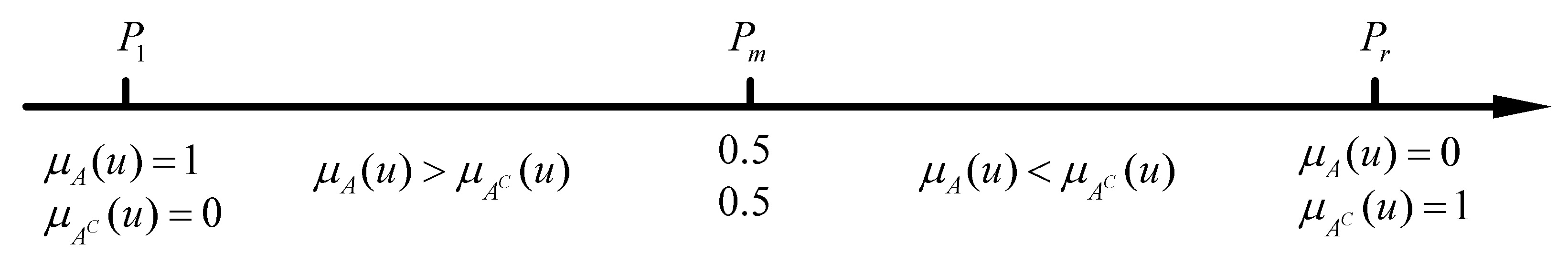
Existing research [28,32] indicates that $U$ is a region by a fuzzy set of opposite concepts and $u$ is a random element in $U$, i.e., $u\in U$. $A$ and $A^C$ are, respectively, defined as continuous intervals expressed by two endpoints 1,0 and 0,1 that correspond to attraction and repellence. The relative membership functions of $u$ that point to $A$ and $A^C$ are ${\mu }_A(u)$ and ${\mu }_{A^C}(u)$, which express the degrees of attraction and repellence, respectively. The relative membership relationship of $A$ and $A^C$ can be expressed by Equation (1) and Figure 1 as follows:

$$\{\begin{array}{l}{\mu }_A,{\mu }_{A^C}:U\to [0,1]\\ u|\to {\mu }_A(u),{\mu }_{A^C}(u)\in [0,1]\end{array}$$

(1)

Figure 1 shows that ${\mu }_A(u)+{\mu }_{A^C}(u)=1$, $0\le {\mu }_A(u)\le 1$, and $0\le {\mu }_{A^C}(u)\le 1$. Therefore, a value can be selected to indicate the changing relationship between ${\mu }_A(u)$ and ${\mu }_{A^C}(u)$.

Let

$$D_A(u)={\mu }_A(u)-{\mu }_{A^C}(u),$$

(2)

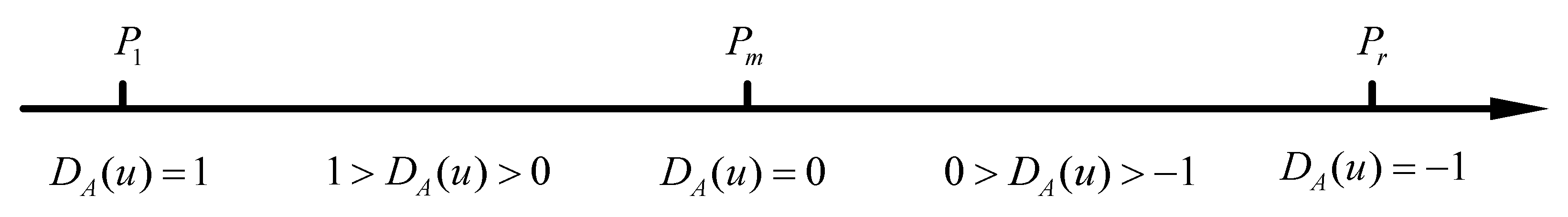
where $D_A(u)$ is defined as the relative difference degree (RDD) of $u$ to $A$. The mapping and diagram of the relative difference function are expressed as Equation (3) and Figure 2, respectively:

$$\{\begin{array}{l}{D}_A(u):D\to [-1,1]\\ u|\to D_A(u)\in [-1,1]\end{array}$$

(3)

The interval $X_0=[a,b]$ is defined as the attracting set of $u$ on the real axis, and $X=[c,d]$ is an extended interval with two endpoint extensions. The interval $X$ included the $X_0$, that is, $X_0\in X$. The relationship between these intervals is illustrated in Figure 3.

The intervals $[c,a]$ and $[b,d]$ are repellent regions of $u$ based on analysis of VFS theory. Therefore, the interval $[a,b]$ is the attractive region of $u$. As shown in Figure 3, point $M$ is a value within the attracting set $[a,b]$ that satisfies the condition $D_A(u)=1$ or ${\mu }_A(u)=1$. In addition, $x$ is a random point in interval $X$ and its RDD is determined by the positions of $x$ and $M$ on the real axis.

When $x$ is located to the left of $M$, the relative difference function can be expressed as:

$$\{\begin{array}{l}{D}_A(u)={\left(\frac{x-a}{M-a}\right)}^{\beta },x\in [a,M]\\ D_A(u)=-{\left(\frac{x-a}{c-a}\right)}^{\beta },x\in [c,a]\end{array}.$$

(4)

When $x$ is located to the right of $M$, the relative difference function can be expressed as:

$$\{\begin{array}{l}{D}_A(u)={\left(\frac{x-b}{M-b}\right)}^{\beta },x\in [M,b]\\ D_A(u)=-{\left(\frac{x-b}{d-b}\right)}^{\beta },x\in [b,d]\end{array}.$$

(5)

Equations (4) and (5) must satisfy the conditions [27,32]:

$$\{\begin{array}{lll}{D}_A(u)=0& & x=aorb\\ D_A(u)=1& & x=M\\ D_A(u)=-1& & x=cord\\ D_A(u)=0& & {\mu }_A(x)={\mu }_{A^C}(x)\\ \beta =1& & \beta isanon-negativeparameter\end{array}.$$

(6)

According to Equation (2) and ${\mu }_A(u)+{\mu }_{A^C}(u)=1$, Equation (7) can be obtained:

$${\mu }_A(u)=(1+D_A(u))/2$$

(7)

Therefore, according to Equations (4), (5), and (7), the RMD function can be derived as follows.

When $x$ is located to the left of $M$, the RMD function can be expressed as:

$$\{\begin{array}{ll}{\mu }_A\left(u\right)=0.5\left[1+\left(\frac{x-a}{M-a}\right)\right],& x\in \left[a,M\right]\\ {\mu }_A\left(u\right)=0.5\left[1-\left(\frac{x-a}{c-a}\right)\right],& x\in \left[c,a\right]\end{array}.$$

(8)

When $x$ is located to the right of $M$, the RMD function can be expressed as:

$$\{\begin{array}{ll}{\mu }_A\left(u\right)=0.5\left[1+\left(\frac{x-b}{M-b}\right)\right],& x\in \left[M,b\right]\\ {\mu }_A\left(u\right)=0.5\left[1-\left(\frac{x-b}{d-b}\right)\right],& x\in \left[b,d\right]\end{array}.$$

(9)

2.1.2. Calculation of the Synthetic Membership Degree

(i) The object to be evaluated is assumed to have $m$ index eigenvalues, given by:

$$X=\left\{x_1,x_2,x_3,\cdots ,x_m\right\}$$

(10)

The indexes to be evaluated can also be assumed to be divided into $c$ levels and the index standard interval matrix for $m$ indexes and $c$ levels is denoted by $I_{ab}$. Then,$I_{ab}$ is constructed as $[a_{ij},b_{ij}]$ and it belongs to the attracting sets. The levels from 1 to $c$ represent an arrangement from superior to inferior. When the index belongs to the larger the better type, $a_{ij}>b_{ij}$. In contrast, when the index belongs to the larger the worse type, $a_{ij}<b_{ij}$. The specific expression of $I_{ab}$ is shown as follows [27,32]:

$$I_{ab}=\left[\begin{array}{ccccc}\left[a_{11},b_{11}\right]& \left[a_{12},b_{12}\right]& \left[a_{13},b_{13}\right]& \cdots & \left[a_{1c},b_{1c}\right]\\ \left[a_{21},b_{21}\right]& \left[a_{22},b_{22}\right]& \left[a_{23},b_{23}\right]& \cdots & \left[a_{2c},b_{2c}\right]\\ \left[a_{31},b_{31}\right]& \left[a_{32},b_{32}\right]& \left[a_{33},b_{33}\right]& \cdots & \left[a_{3c},b_{3c}\right]\\ ⋮& ⋮& ⋮& \ddots & ⋮\\ \left[a_{m1},b_{m1}\right]& \left[a_{m2},b_{m2}\right]& \left[a_{m3},b_{m3}\right]& \cdots & \left[a_{mc},b_{mc}\right]\end{array}\right]=(\left[a_{ih},b_{ih}\right])=({\left[a,b\right]}_{ih})$$

(11)

According to $I_{ab}$, the extended interval is constructed $[c_{ij},d_{ij}]$ and can also be called the indicator variable interval matrix $I_{cd}$. The conversion relationship between $I_{ab}$ and $I_{cd}$ is shown as follows [28,34]:

$$\left[c_{ih},d_{ih}\right]=\{\begin{array}{ll}\left[a_{ih-1},b_{ih+1}\right],& h-1>0,h<c\\ \left[a_{i1},b_{ih+1}\right],& h-1=0\\ \left[a_{ih-1},b_{ic}\right],& h=c\end{array}$$

(12)

Therefore, the specific expression for $I_{cd}$ is shown as follows:

$$I_{cd}=\left[\begin{array}{ccccc}\left[c_{11},d_{11}\right]& \left[c_{12},d_{12}\right]& \left[c_{13},d_{13}\right]& \cdots & \left[c_{1c},d_{1c}\right]\\ \left[c_{21},d_{21}\right]& \left[c_{22},d_{22}\right]& \left[c_{23},d_{23}\right]& \cdots & \left[c_{2c},d_{2c}\right]\\ \left[c_{31},d_{31}\right]& \left[c_{32},d_{32}\right]& \left[c_{33},d_{33}\right]& \cdots & \left[c_{3c},d_{3c}\right]\\ ⋮& ⋮& ⋮& \ddots & ⋮\\ \left[c_{m1},d_{m1}\right]& \left[c_{m2},d_{m2}\right]& \left[c_{m3},d_{m3}\right]& \cdots & \left[c_{mc},d_{mc}\right]\end{array}\right]=(\left[c_{ih},d_{ih}\right])=({\left[c,d\right]}_{ih})$$

(13)

(ii) The point $M$ must be calculated. The foregoing description indicates that point $M_{ih}$ is a value within the attracting set $[a_{ih},b_{ih}]$ that satisfies the condition $D_A(u)=1$ or ${\mu }_A(u)=1$. The first level indicates that point $M_{i1}$ is equal to $a_{i1}$, while the c-th level indicates that point $M_{ic}$ is equal to $b_{ic}$. However, two commonly used calculation methods for the value of point $M_{ih}$ are available for levels $2,3,4,\cdots ,m-1$. (a) The midpoint of the standard interval $[a_{ih},b_{ih}]$ is used as the value of point $M_{ih}$, which can be expressed by Equation (14) [33] This method is simple and straightforward; however, the meaning of relative membership is unclear for non-intermediate levels. (b) According to the definition of a VFS, when $M$ is a linear change, the general calculation formula for the value of point $M_{ih}$ is Equation (15) when the changing state of $M_{ih}$ is linear change [39]. This method can efficiently solve the situation in which the meaning of relative membership of non-intermediate level is unclear when point $M_{ih}$ is calculated as follows:

$$M_{ih}=(a_{ih}+b_{ih})/2$$

(14)

$$M_{ih}=\frac{c-h}{c-1}{a}_{ih}+\frac{h-1}{c-1}{b}_{ih}$$

(15)

(iii) The RMD ${\mu }_A{(u)}_{ih}$ of each index to the h-th level can be calculated according to Equations (8)–(11), (13,) and (15). The ${\mu }_A{(u)}_{ih}$ of all the indexes to be evaluated can be calculated and integrated, and then the RMD matrix of the m indexes to the c levels can be obtained as follows:

$${\mu }_A{(u)}_{m\times c}=\left[\begin{array}{ccccc}{\mu }_A{(u)}_{11}& {\mu }_A{(u)}_{12}& {\mu }_A{(u)}_{13}& \cdots & {\mu }_A{(u)}_{1c}\\ {\mu }_A{(u)}_{21}& {\mu }_A{(u)}_{22}& {\mu }_A{(u)}_{23}& \cdots & {\mu }_A{(u)}_{2c}\\ {\mu }_A{(u)}_{31}& {\mu }_A{(u)}_{32}& {\mu }_A{(u)}_{33}& \cdots & {\mu }_A{(u)}_{3c}\\ ⋮& ⋮& ⋮& \ddots & ⋮\\ {\mu }_A{(u)}_{m1}& {\mu }_A{(u)}_{m2}& {\mu }_A{(u)}_{m3}& \cdots & {\mu }_A{(u)}_{mc}\end{array}\right]$$

(16)

(iv) The synthetic membership degree (SMD) can be calculated using the variable fuzzy synthetic evaluation model. This model was developed from the variable fuzzy clustering models, the variable fuzzy recognition models, and the variable fuzzy optimization models. The complete derivation process is not presented here due to space constraints. The model is expressed as follows:

$$u_h^{\prime }={\left\{1+{\left[\frac{{\displaystyle \sum _{i=1}^m{\left[{\omega }_i\left(1-{\mu }_A{\left(x_i\right)}_h\right)\right]}^p}}{{\displaystyle \sum _{i=1}^m{\left[{\omega }_i{\mu }_A{\left(x_i\right)}_h\right]}^p}}\right]}^{\frac{\alpha }{p}}\right\}}^{-1}$$

(17)

where $m$ is the number of recognition indicators; ${\omega }_i$ is the weight value of the index; h is the grade parameter; $p$ is the variable distance parameter, usually taking $p=1$ as the Hamming distance and $p=2$ as the Euclidean distance; and $\alpha$ is the rule parameter for model optimization, where $\alpha =1$ and $\alpha =2$ corresponds to the least single method and least squares method, respectively.

Four corresponding combinations can be generated according to the values of $\alpha$ and $p$, and each combination can be calculated to obtain a SMD set.

(v) The SMD matrix $U^{\prime }$ can be obtained using Equation (17) under the four combinations, and $U$ can be obtained by normalizing $U^{\prime }$. According to the definition of the level eigenvalues in the VFS, Equations (18), (19), and (20) can be obtained as follows:

$$H=\left(1,2,3,\cdots ,c\right)•U$$

(18)

$$\overline{H}={\displaystyle \sum _{t=1}^4{H}_t/4}.$$

(19)

where $t$ represents the four parameter combinations, $t=1,2,3,4$.

$$\{\begin{array}{ll}1.0\le H(u_0)\le 1.5,& \in Grade1\\ h-0.5<H(u_0)\le h,& \in Gradeh,Tendto(h-1)(h=2,3,4,\cdots ,c-1)\\ h<H(u_0)\le h+0.5,& \in Gradeh,Tendto(h+1)(h=2,3,4,\cdots ,c-1)\\ c-0.5<H(u_0)\le c,& \in Gradec\end{array}$$

(20)

Finally, the level corresponding to the object to be evaluated can be accurately calculated using Equation (20).

2.2. Improvement of Traditional Variable Fuzzy Set

Analysis of the traditional VFS calculation process reveals that the RMD calculation for each index is complex and laborious. This manifests as follows:

(i)

It is necessary to determine the positional relationship between the values of index $x$ and point $M$ at each level frequently when using Equations (8) and (9) to calculate the RMD.

(ii)

The selection accuracy of the value of point $M$ directly determines the accuracy of the RDD. Moreover, it is convenient to use Equations (14) or (15) for the calculation when dealing with quantitative problems. However, the core meaning for the treatment of qualitative indexes cannot be expressed clearly and accurately based on the equations alone. Thus, the assignment experts must have excellent assignment experience and ability. Otherwise, the lack of such requirements will directly lead to the deviation of the calculation results.

(iii)

Fuzziness can be well reflected by VFS, but the determination of the RDD of its core parameters is highly dependent on expert experience; thus, the calculation of qualitative indexes is prone to serious deviations [40,41]. Therefore, it is necessary to improve VFSs to utilize their accuracy when dealing with qualitative and quantitative combinability problems.

The objective of this study is to develop a social impact assessment for dam breaks. However, these are low frequency and high loss events, so it is difficult to obtain large quantities of data. Therefore, the widely used grey system theory (GST) is introduced to improve the VFS.

Deng (1989) [42] proposed the GST, which is used to deal with the problem of uncertainty. It focuses on fuzzy problems where the sample size is small, and the information is poor [43]. Similar to most system analysis methods, grey relational degree (GRD) is used as the core parameter of GST to express the processing results for various fuzzy issues. Moreover, grey relational analysis (GRA) is required to achieve this result. The basic principle of GRA is to identify the degree of correlation between many factors based on the geometric pattern similarity of the sequence curve. The greater the similarity of the curves, the higher the correlation between the sequences.

GST has been applied in many fields due to its good characteristics and continuous development by many scholars. These fields include: optimal plan selection for energy planning [43,44,45], optimal supplier selection in supply chains [46], traffic safety decisions for ship navigation maneuvers [47], reasonable distribution and prediction of urban heating [48,49], performance prediction for concrete materials [50,51,52], assessment of regional agricultural water and soil resources system [53], and comprehensive evaluation of the effectiveness of coal-fired power plants [54]. GRA has made remarkable progress in these applications and the results are reliable and accurate. Therefore, the improvements in the VFS in this study is achieved using the GRA in the GST.

2.2.1. Basic Concepts of Grey Relational Analysis

The basic idea of GRA is to determine close relationships between sequences according to the similarity in the geometric shapes of their sequence curves. When curves are close, there is a strong correlation between the sequences and vice versa [54].

Suppose the system characteristic behavior sequence (i.e., the reference sequence) is $X_0=(x_0(1),x_0(2),x_0(3),\cdots ,x_0(n))$, then the related factor sequence (i.e., the compared sequence) can be expressed as follows [51]:

$$\begin{array}{c}{X}_1=(x_1(1),x_1(2),x_1(3),\cdots ,x_1(n))\hfill \\ \cdots \cdots \\ X_i=(x_i(1),x_i(2),x_i(3),\cdots ,x_i(n))\hfill \\ \cdots \cdots \\ X_m=(x_m(1),x_m(2),x_m(3),\cdots ,x_m(n))\hfill \end{array}$$

(21)

At this time, Equation (22) can be expressed as follows:

$$\gamma (X_0,X_i)=\frac{1}{n}{\displaystyle \sum _{k=1}^n\gamma (x_0(k),x_i(k))}$$

(22)

Therefore, $\gamma (X_0,X_i)$ in Equation (22) is the GRD between $X_0$ and $X_i$, and Equation (22) must satisfy the following conditions [46,51]:

(i) Normalization

$$0<\gamma (X_0,X_i)\le 1,\gamma (X_0,X_i)=1\Leftarrow X_0=X_i;$$

(ii) Wholeness

For $X_i,X_j\in X=\left\{X_s|s=0,1,2,3,\cdots ,m;m\ge 2\right\}$, then $\gamma (X_i,X_j)\ne \gamma (X_j,X_i),i\ne j$ can be obtained;

(iii) Even pair symmetry

For $X_i,X_j\in X$, then $\gamma (X_i,X_j)=\gamma (X_j,X_i)\iff X=\left\{X_i,X_j\right\}$ can be obtained;

(iv) Proximity

As $\left|x_0(k)-x_i(k)\right|$ decreases, the $\gamma (x_0(k),x_i(k))$ increases.

In Equation (22), the $\gamma (x_0(k),x_i(k))$ may be expressed as follows:

$$\gamma (x_0(k),x_i(k))=\frac{\underset{i}{\min }\underset{k}{\min }\left|x_0(k)-x_i(k)\right|+\xi \underset{i}{\max }\underset{k}{\max }\left|x_0(k)-x_i(k)\right|}{\left|x_0(k)-x_i(k)\right|+\xi \underset{i}{\max }\underset{k}{\max }\left|x_0(k)-x_i(k)\right|}$$

(23)

where $k=1,2,3,\cdots ,n$, $i=1,2,3,\cdots ,m$; $\gamma (x_0(k),x_i(k))$ is called the relational coefficient; and $\xi$ is the resolution coefficient where, $\xi \in (0,1)$ and it is generally taken that $\xi =0.5$.

2.2.2. Similarity Analysis of the core parameters

The social impact assessment system for a dam break should combine the characteristics of the dam-break event with uncertainty and randomness. As a theoretical method of dealing with the problem of uncertainty, VFSs and GST are applicable. However, both have their own advantages and disadvantages. Herein, a comparative analysis of the core parameters of the GRD and RDD are presented. There is a quantitative relationship between the degree of the relative difference and relative membership, as shown by Equation (7). Therefore, the RDD can completely represent the RMD at the core parameter level.

The index characteristics of the GRD are portrayed by the relational coefficient (that is, Equation (23)). The analysis of Equation (23) shows that the essential connotation of the relational coefficient is the absolute value of the difference between the reference and compared sequences. The relational coefficient is also a comparison of the relative difference between the two sets of index data. According to the RDD presented in the previous section and in Equation (2), the core connotation of the RDD is “attraction minus repellence”. The RDD is also the magnitude of the correlation between the two sets of data. Therefore, the GRD and the RDD have similar essential connotations.

The disadvantages of VFSs have been described in previous sections. Analysis of these disadvantages shows that they are concentrated in the RMD calculation. However, GRA has several advantages as follows:

(i) GRA has an excellent effect on systematic reviews that involve a large amount of unknown information. It can also provide excellent solutions for evaluation indexes that are difficult to quantify or count. In the evaluation process, the effect of human factors can be excluded to obtain objective and accurate results. Therefore, GRA can effectively solve the problem of determining the RDD by relying on expert experience and the inability to accurately characterize qualitative indicators.

(ii) The GRA model is simple and the fast calculation process can easily be mastered by an operator. Determining the positional relationship between the values of index $x$ and the value of point $M$ at each level is often necessary for the RMD calculation in VFSs. The calculation process of the GRD is simple. In addition, the GRA effectively avoids the difficult problem of determining the value of point $M$ when analyzing qualitative problems.

(iii) GRA does not require a large amount of sample data in its application. Moreover, it can provide a scientific and correct evaluation of the entire evaluation system based on a small amount of representative data with reliable results. It is difficult to obtain a large amount of index data for dam break social impact assessments. Therefore, the low data requirements are an important consideration.

However, GRA also has shortcomings, particularly surrounding the determination of the evaluation results by simply using a combination of index weights and relational coefficients. This approach is similar to the principle of maximum membership degree in fuzzy mathematics. However, information loss is encountered when using these principles for level judgment. VFSs use variable parameter combinations to determine the SMD vector for each parameter combination and calculate the corresponding level eigenvalues. Finally, the evaluation results are determined by analyzing the level eigenvalues, and this method retains all information to the largest extent.

By analyzing the advantages and disadvantages of the two methods, a new method is proposed to combine the most desirable features. That is, the GRD calculation process is used instead of the RDD process.

2.2.3. Calculation Steps of the New Method

Step 1 Determination of the evaluation object and index sets;

Suppose $m$ evaluation objects and $n$ evaluation indexes are available, then the original index data matrix can be expressed as follows:

$$A={\left[\begin{array}{ccccc}{a}_{11}& a_{12}& a_{13}& \cdots & a_{1n}\\ a_{21}& a_{22}& a_{23}& \cdots & a_{2n}\\ a_{31}& a_{32}& a_{33}& \cdots & a_{3n}\\ ⋮& ⋮& ⋮& \ddots & ⋮\\ a_{m1}& a_{m2}& a_{m3}& \cdots & a_{mn}\end{array}\right]}_{m\times n}$$

(24)

where $a_{ij}$ represents the j-th index value of the i-th evaluation object $a_i$.

Step 2 Determination of the index reference value;

$$A_0=\left(a_{01},a_{02},a_{03},\cdots ,a_{0n}\right)$$

(25)

where $a_{0i}\left(i=1,2,3,\cdots ,n\right)$ represents the optimal value of the i-th index.

Matrix $B$ can be formed based on the original index data and reference values, and the expression is as follows:

$$B={\left[\begin{array}{ccccc}{a}_{01}& a_{02}& a_{03}& \cdots & a_{0n}\\ a_{11}& a_{12}& a_{13}& \cdots & a_{1n}\\ a_{21}& a_{22}& a_{23}& \cdots & a_{2n}\\ a_{31}& a_{32}& a_{33}& \cdots & a_{3n}\\ ⋮& ⋮& ⋮& \ddots & ⋮\\ a_{m1}& a_{m2}& a_{m3}& \cdots & a_{mn}\end{array}\right]}_{\left(m+1\right)\times n}$$

(26)

Step 3 Dimensionless processing of index values;

Indexes cannot be compared directly and the differences between them cannot be determined correctly because the evaluation indexes involved in social impact assessments for dam breaks have many different units. Therefore, all the initial index values in the evaluation process must be dimensionless.

Assuming that the maximum value of the j-th index $a_j$ is $S_j$, then:

$$S_j=\max (a_j)$$

(27)

$$x_{ij}=a_{ij}/S_j$$

(28)

where $x_{ij}$ is the dimensionless value of $a_{ij}$.

The result of dimensionless processing on the original indicator matrix $B$ is matrix $X$:

$$X={\left[\begin{array}{ccccc}{x}_{01}& x_{02}& x_{03}& \cdots & x_{0n}\\ x_{11}& x_{12}& x_{13}& \cdots & x_{1n}\\ x_{21}& x_{22}& x_{23}& \cdots & x_{2n}\\ x_{31}& x_{32}& x_{33}& \cdots & x_{3n}\\ ⋮& ⋮& ⋮& \ddots & ⋮\\ x_{m1}& x_{m2}& x_{m3}& \cdots & x_{mn}\end{array}\right]}_{\left(m+1\right)\times n}$$

(29)

Step 4 Calculation of the difference in the sequence, maximum difference, and minimum difference;

The difference in the sequence can be expressed as follows:

$${\Delta }_{0i}=\left({\Delta }_{0i}(1),{\Delta }_{0i}(2),{\Delta }_{0i}(3),\cdots ,{\Delta }_{0i}(n)\right)$$

(30)

where ${\Delta }_{0i}(j)=\left|x_{0j}-x_{ij}\right|,i=1,2,3,\cdots ,m;j=1,2,3,\cdots ,n$.

The maximum and minimum difference are given by:

$${\Delta }_{\max }=\underset{i}{\max }\underset{j}{\max }\left\{{\Delta }_{0i}(j)\right\}$$

(31)

$${\Delta }_{\min }=\underset{i}{\min }\underset{j}{\min }\left\{{\Delta }_{0i}(j)\right\}$$

(32)

where $i=1,2,3,\cdots ,m;j=1,2,3,\cdots ,n$.

Step 5 Calculation of the grey relational coefficient;

According to the dimensionless index and optimal reference values, the relational coefficient of each index relative to the optimal value can be calculated as follows:

$${\gamma }_{ij}=\frac{{\Delta }_{\min }+\xi {\Delta }_{\max }}{{\Delta }_{0i}(j)+\xi {\Delta }_{\max }}$$

(33)

where $i=1,2,3,\cdots ,m;j=1,2,3,\cdots ,n$; $\xi$ is the resolution coefficient, $\xi \in (0,1)$, which is generally taken as $\xi =0.5$.

Step 6 Construction of the RMD;

Combining the description of the quantitative relationship and the core meaning of the RMD, RDD, and GRD, means that the value of the RDD can be expressed by the value of the grey relational coefficient. Therefore, the RDD matrix can be expressed as follows:

$$D={\left[\begin{array}{ccccc}{\gamma }_{11}& {\gamma }_{12}& {\gamma }_{13}& \cdots & {\gamma }_{1m}\\ {\gamma }_{21}& {\gamma }_{22}& {\gamma }_{23}& \cdots & {\gamma }_{2m}\\ {\gamma }_{31}& {\gamma }_{32}& {\gamma }_{33}& \cdots & {\gamma }_{3m}\\ ⋮& ⋮& ⋮& \ddots & ⋮\\ {\gamma }_{n1}& {\gamma }_{n2}& {\gamma }_{n3}& \cdots & {\gamma }_{nm}\end{array}\right]}_{n\times m}$$

(34)

Combining Equations (7) and (34) allows the normalized RMD matrix to be expressed as follows:

$$\mu {(u)}_{n\times m}={\left[\begin{array}{ccccc}\mu {(u)}_{11}& \mu {(u)}_{12}& \mu {(u)}_{13}& \cdots & \mu {(u)}_{1m}\\ \mu {(u)}_{21}& \mu {(u)}_{22}& \mu {(u)}_{23}& \cdots & \mu {(u)}_{2m}\\ \mu {(u)}_{31}& \mu {(u)}_{32}& \mu {(u)}_{33}& \cdots & \mu {(u)}_{3m}\\ ⋮& ⋮& ⋮& \ddots & ⋮\\ \mu {(u)}_{n1}& \mu {(u)}_{n2}& \mu {(u)}_{n3}& \cdots & \mu {(u)}_{nm}\end{array}\right]}_{n\times m}.$$

(35)

Step 7 Determination of the index weight values;

The accuracy of the index weight values affects the final evaluation results. Therefore, this study employed the analytic hierarchy process (AHP) method, which is widely used to calculate the index weight value. The principle and calculation steps of this method are detailed elsewhere [37,54,55,56].

Step 8 Calculation of the SMD;

The SMD can be calculated by substituting Equation (35) into Equation (17).

Step 9 Judgment of evaluation results.

The SMD matrix $U^{\prime }$ can be obtained via Step 8 under the four combinations, and $U$ can be obtained by normalizing $U^{\prime }$. Finally, the evaluation results can be obtained using Equations (18)–(20).

3. Evaluation Index System

The previous sections highlighted the considerable importance of social impact assessments for dam breaks. Moreover, the establishment of a scientific evaluation system guides the evaluation results. However, the assessment of and research into the social impact of dam breaks are still in their infancy across the international community. Furthermore, there is no widely accepted definition of the social impact of dam breaks. Therefore, the social impact of other industries or natural disasters and the existing research results of scholars can provide a reference for the establishment of a social impact assessment index system for dam breaks in this paper [57,58,59].

3.1. Establishment of Evaluation Indexes

Social impact is a measure of the human spiritual injuries and social unrest caused by the loss of life and property, destruction of factories and cultural industries, and damage to the infrastructure required for daily life. Here, these aspects are considered for dam breaks.

When a dam is breached, water suddenly flows at high speed, entraining soil, gravel, and sediments and the destruction is equivalent to that of a huge flood peak. The analysis of the possible social impact consequences of a flood caused by a dam break is shown in

Table 1. Major behavior of a dam break and possible social impact [57].

Major Behavior of a Dam Break	Possible Consequences
Large- and high-speed sudden water flows containing soil, gravel, and sediments	Loss of human life and property
	Damage to residential and basic security facilities
	Damage to road, traffic, and communication facilities
	Social unrest and turmoil caused by human panic
	Damage to cultural heritage and cultural landscape

.

In addition to the situation in the downstream area, the scale of the dam has a substantial effect on the destructive power of the flood caused by a dam break. Therefore, the height of dam and the capacity of the reservoir should be considered as part of the evaluation.

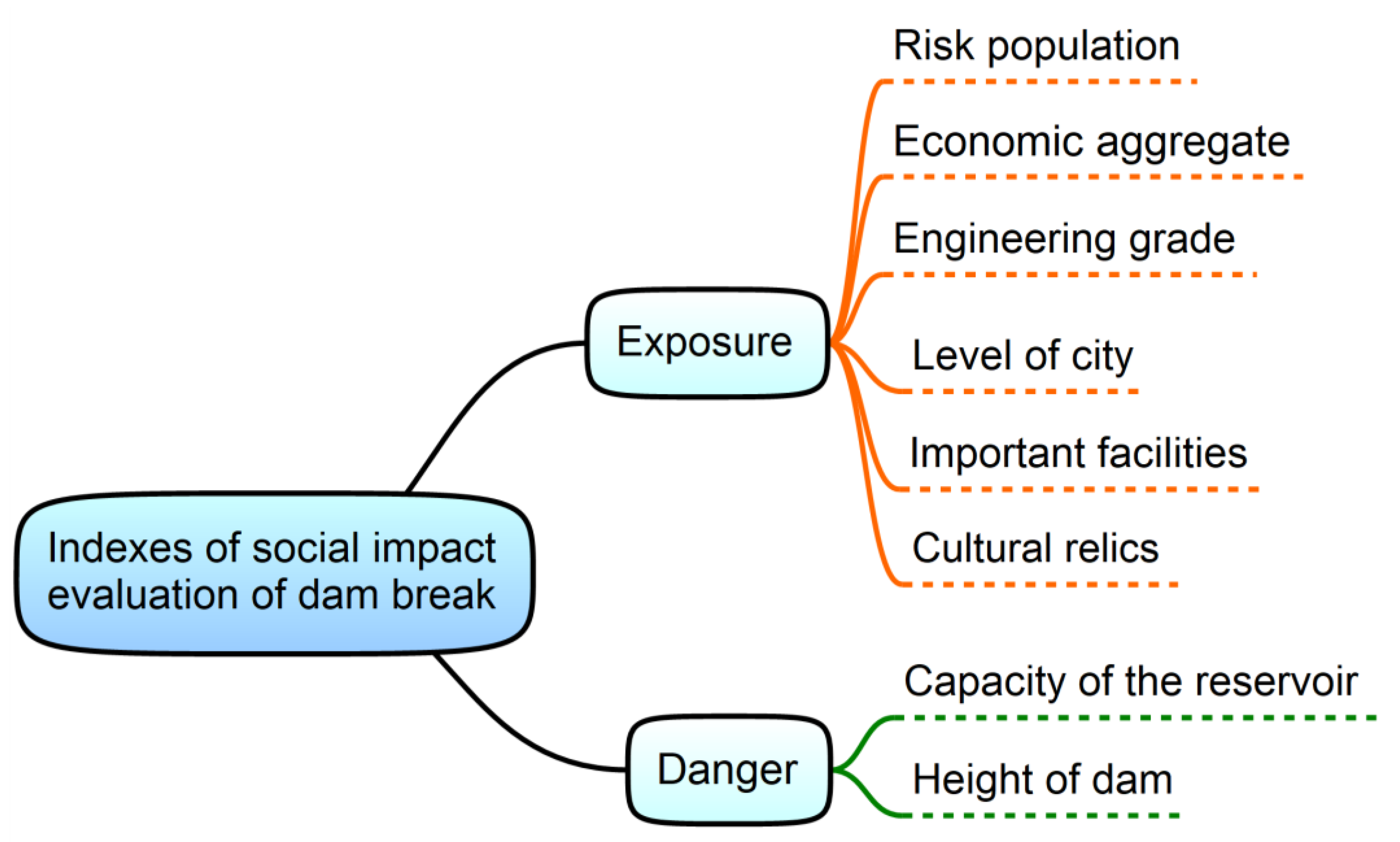
It is difficult to scientifically sort and analyze all of the factors that affect the social impact of a dam break due to their transient and complex behaviors. Therefore, this study relies on work by previous scholar’s research [58] and concentrates on the social impact characteristics and dam break behavior [7,20,21,24,59]. A set of representative indicators can be obtained by analysis and sorting according to the principles of combining science, typicality, practicality, and qualitive and quantitative data. These indicators are used as the index system of the social impact assessment for dam breaks in this study. The index system is shown in Figure 4.

3.2. Index Classification and Gradation

The study references existing research from this and other industries. The results are based on the “Report on Production Safety Accident and Regulations of Investigation and Treatment” promulgated by the State Council of the People’s Republic of China and “Guidelines for Emergency Preparedness Plan of Reservoir Dam Safety Management” issued by the Ministry of Water Resources the People’s Republic of China in combination with the unique behavioral attributes of dam breaks. Each of the evaluation indexes are divided into five levels from light to heavy, i.e., slight, ordinary, medium, serious, and extremely serious. The evaluation levels for the quantitative indexes, height of dam and capacity of the reservoir, are determined using the “Standard for Classification and Flood Control of Water Resources and Hydroelectric Project” as a reference. The evaluation level for the quantitative index risk population is determined based on the concept of population density, i.e., it depends on the total population of the affected area and the units are people per square kilometer. Economic aggregate is another quantitative index; its evaluation level is determined based on the total economic value of the affected area and the units are ten thousand RMB. These quantitative indexes can be quantified through measurements or surveys.

The four remaining indicators are all qualitative and dimensionless. According to the principle of scientific and average distribution, the corresponding evaluation level from 0 to 100 can be determined by intervals. In this study, five evaluation levels are used, and the judgement interval is divided into five equal parts which are assigned to the evaluation levels in order.

The classification and evaluation levels corresponding to each indicator can be determined through specific analysis of the characteristics of each indicator [58,59]. It is crucial to explain the judgement standards and connotations of the evaluation levels for each index comprehensively, so that experts can judge the evaluation levels correctly.

Table 2. Classification and grade suggestions for indexes of danger.

Evaluation Level	Index of Danger
	Capacity of the Reservoir (Unit: Ten Thousand m3)	Height of Dam (Unit: m)
Slight	(10,102)	(0,10)
Ordinary	(102,103)	(10,20)
Medium	(103,104)	(20,30)
Serious	(104,105)	(30,60)
Extremely serious	(105,106)	(60,100)

and

Table 3. Classification and grade suggestions for indexes of exposure.

Evaluation Level	Index of Exposure
	Risk Population (Unit: Ten Thousand People)	Economic Aggregate (Unit: Ten Thousand RMB)	Engineering Grade	The Level of City	Important Facilities	Cultural Relics
Slight	(0,50)	Extremely underdeveloped economy (10,102)	Fifth-class project (0,20)	Scattered residents (0,20)	Transportation, transmission, oil, and gas facilities of a town level (0,20)	General cultural relics, works of art, animals, and plants (0,20)
Ordinary	(50,200)	Underdeveloped economy (102,103)	Fourth-class project (20,40)	Village (20,40)	Transportation, transmission, oil, and gas facilities of a county level (20,40)	Cultural relics, works of art, animals, and plants of a county level (20,40)
Medium	(200,400)	Medium economy (103,104)	Third-class project (40,60)	Seat of a township government (40,60)	Transportation, transmission, oil, and gas facilities of a municipal level (40,60)	Cultural relics, works of art, animals, and plants of provincial and municipal levels (40,60)
Serious	(400,600)	Developed economy (104,106)	Second-class project (60,80)	Seat of a county or prefecture-level city government (60,80)	Transportation, transmission, oil, and gas facilities of a provincial level (60,80)	Cultural relics, works of art, animals, and plants of a national level (60,80)
Extremely serious	(600,1200)	Extremely developed economy (106,108)	First-class project (80,100)	National capital city or municipality or provincial capital or key development city (80,100)	Transportation, transmission, oil, and gas facilities of a national level (80,100)	Cultural relics, works of art, animals, and plants of an international level (80,100)

present some classification and grade suggestions for the danger and exposure indexes.

4. Result

The Liujiatai Reservoir was considered as an example and the improved VFS was applied to evaluate the social impact of a dam break to verify the accuracy and reliability of the proposed method.

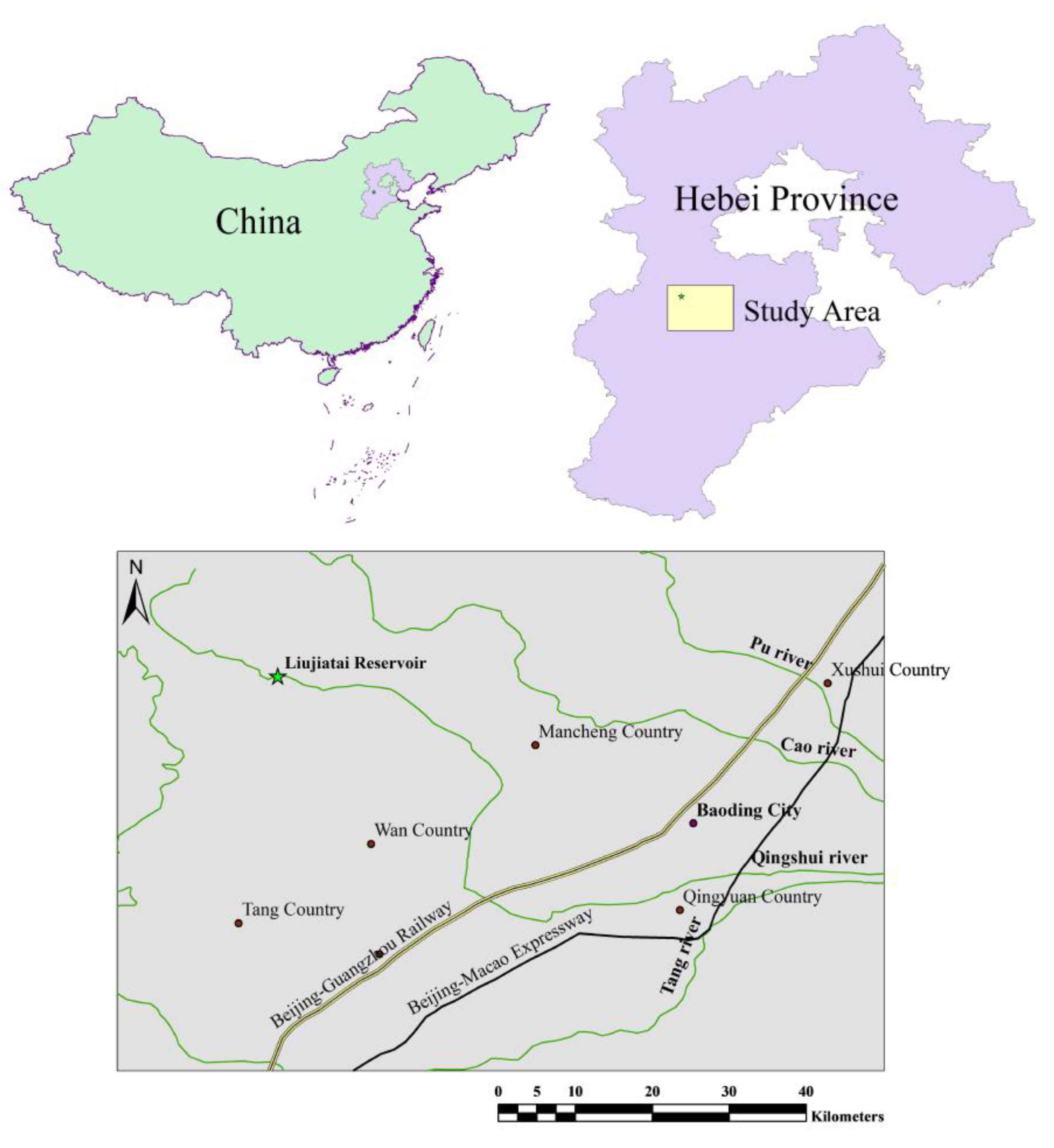
The Liujiatai Reservoir is located in Yi County, Baoding City, Hebei Province, China. The reservoir has a controlled drainage area of 174 km² and its total capacity is 40,500,000 m³, which makes it a medium-sized reservoir. The dam is mainly constructed from clay and silty clay. The dam has a maximum height of 35.8 m and the top is 295 m long and 5 m wide. The national railway trunk lines of Beijing-Guangzhou Railway, Beijing-Shijiazhuang Railway, and national highway trunk line Beijing-Hong Kong-Macao Expressway are located approximately 30 km east of Yi County. Meanwhile, the Beijing-Yuanping Railway passes through the north of Yi County. There are six national key cultural relic protection units and eight provincial key cultural relic protection units in Yi county. In addition, there are world-class cultural relics in the form of the Western Royal Tombs of the Qing Dynasty and the Jingke Pagoda which was built in the third year of Qiantong in the Liao Dynasty (i.e., 1103 A.D).

The Liujiatai Reservoir broke at 4 a.m. on 8 August 1963. During the breach, the maximum flow was approximately 28,600 m³/s and the average flow was 23,000 m³/s. Investigation revealed that the water caused damage to varying degrees across 68 villages in Yixian County, Mancheng County, Shunping County, and Baoding City within 30 km downstream of the reservoir. In these areas, a total of 64,941 people were affected, and the total economic loss was 15,000,000 RMB.

A schematic showing the location of the Liujiatai Reservoir prior to its failure was produced using relevant historical data, as shown in Figure 5.

4.1. Weights and Values of the Indexes

It is necessary to calculate the weight of each indicator to evaluate the social impact of a dam break accurately and comprehensively. In this study, the weight value of each index was calculated using the AHP method introduced in Section 2.2.3. This method is excellent for processing mixed qualitative and quantitative problems. In general, experts compare the mutual importance of indicators, establish a judgment matrix after scoring, and then conduct the processes of importance ranking and a consistency check. Finally, the weight of an evaluation index can be calculated. The index weights for the evaluation system are shown in

Table 4. Weights of each index in the evaluation system.

Evaluation System	Target Layer (${\mathit{\omega }}_{\mathit{i}}$)	Index Layer	Weights (${\mathit{\omega }}_{\mathit{i}\mathit{j}}$)	Weights (${\mathit{\omega }}_{\mathit{n}}$)
Indexes of social impact assessment of dam break	Danger (${\omega }_1=0.53$)	Height of dam	0.400	0.212
		Capacity of the reservoir	0.600	0.318
	Exposure (${\omega }_2=0.47$)	Risk population	0.130	0.061
		Economic aggregate	0.196	0.092
		Engineering grade	0.217	0.102
		Level of city	0.174	0.082
		Important facilities	0.109	0.051
		Cultural relics	0.174	0.082

Notes: ${\omega }_n$ represents the weight value of each index in the index layer relative to the evaluation system, ${\omega }_n={\omega }_i\times {\omega }_{ij}$.

.

Dam breaks are low-probability events, so it is difficult to obtain a considerable amount of data. Moreover, social impact assessments are predictive assessments that involve many qualitative indicators. Therefore, the indicator data in this study were obtained through expert judgment and scoring based on Table 3, the actual project, statistical analysis of data, and reference to relevant literature. This step ensures that the data values to be evaluated accurately reflect the actual situation. Thus, the index values of the dam break social impact assessment for the Liujiatai Reservoir were determined, as shown in

Table 5. Values of various indexes of the dam break social impact assessment for the Liujiatai Reservoir.

Evaluation Indexes	Actual Status Description	Value of Evaluation (${\mathit{x}}_{\mathit{i}}$)
Height of dam	Actual value	35.8
Capacity of the reservoir	Actual value	4050
Risk population	Actual value	373
Economic aggregate	Actual value	1500
Engineering grade	A third-class project, close to second-class	41.5
level of city	Baoding city is a key development city downstream of the reservoir	84
Important facilities	Many national railway and highway trunks are found downstream of the reservoir	91.5
Cultural relics	The downstream area contains many items of national and world-class cultural heritage	97.5

.

4.2. Calculating the Relative Membership Degree of Indexes

An improved VFS was used in this paper to conduct a social impact assessment for the dam break at the Liujiatai Reservoir. Combined with a review of the calculation steps of the proposed method, the grey relational coefficient was calculated first.

The median of each index evaluation interval in Table 2 and Table 3 were used to construct the original index data matrix, which is expressed using Equation (24) to ensure that the data can be used to the greatest extent. According to Table 3 and Table 5 and Equations (24)–(33), the calculation result of the gray correlation coefficient matrix can be expressed as Equation (36) as follows:

$$\gamma =\left[\begin{array}{cccccccc}0.5650& 0.9857& 0.5639& 1.0000& 0.5883& 0.3782& 0.3557& 0.3396\\ 0.6579& 0.9875& 0.6447& 1.0000& 0.7965& 0.4546& 0.4225& 0.4000\\ 0.7874& 0.9948& 0.8604& 0.9999& 0.8411& 0.5696& 0.5202& 0.4865\\ 0.8130& 0.8437& 0.7799& 0.9805& 0.6123& 0.7627& 0.6767& 0.6207\\ 0.4751& 0.3350& 0.4606& 0.3333& 0.4813& 0.8824& 0.9678& 0.8572\end{array}\right]$$

(36)

According to the definition in step 6 of Section 2.2.3, the RDD and RMD matrixes can be expressed as Equation (37) and Equation (38), respectively, as follows:

$$D=\left[\begin{array}{ccccc}0.5650& 0.6579& 0.7874& 0.8130& 0.4751\\ 0.9857& 0.9875& 0.9948& 0.8437& 0.3350\\ 0.5639& 0.6447& 0.8604& 0.7799& 0.4606\\ 1.0000& 1.0000& 0.9999& 0.9805& 0.3333\\ 0.5883& 0.7965& 0.8411& 0.6123& 0.4813\\ 0.3782& 0.4546& 0.5696& 0.7627& 0.8824\\ 0.3557& 0.4225& 0.5202& 0.6767& 0.9678\\ 0.3396& 0.4000& 0.4865& 0.6207& 0.8572\end{array}\right]$$

(37)

$$\mu \left(u\right)=\left[\begin{array}{ccccc}0.7825& 0.8290& 0.8937& 0.9065& 0.7375\\ 0.9929& 0.9937& 0.9974& 0.9219& 0.6675\\ 0.7820& 0.8224& 0.9302& 0.8900& 0.7303\\ 1.0000& 1.0000& 0.9999& 0.9902& 0.6667\\ 0.7941& 0.8982& 0.9206& 0.8061& 0.7406\\ 0.6891& 0.7273& 0.7848& 0.8814& 0.7412\\ 0.6779& 0.7113& 0.7601& 0.8384& 0.9839\\ 0.6698& 0.7000& 0.7432& 0.8104& 0.9286\end{array}\right]$$

(38)

Therefore, the normalized RMD matrix can be expressed as follows:

$${\mu }^{\prime }{(u)}_{8\times 5}=\left[\begin{array}{ccccc}0.1886& 0.1998& 0.2154& 0.2185& 0.1778\\ 0.2171& 0.2173& 0.2181& 0.2016& 0.1460\\ 0.1882& 0.1979& 0.2239& 0.2142& 0.1758\\ 0.2147& 0.2147& 0.2147& 0.2126& 0.1432\\ 0.1909& 0.2159& 0.2213& 0.1938& 0.1781\\ 0.1713& 0.1807& 0.1950& 0.2190& 0.2339\\ 0.1707& 0.1791& 0.1914& 0.2111& 0.2477\\ 0.1739& 0.1817& 0.1930& 0.2104& 0.2411\end{array}\right]$$

(39)

4.3. Determining the Evaluation Level

The SMD results under the four parameter combinations can be calculated according to Equation (17). The matrix of normalized SMD of indexes can be represented by $U$, as is expressed in Equation (40) as follows:

$$U^{\prime }=\left[\begin{array}{ccccc}0.1967& 0.2041& 0.2126& 0.2088& 0.1778\\ 0.2040& 0.2089& 0.2149& 0.2067& 0.1655\\ 0.1912& 0.2086& 0.2295& 0.2199& 0.1508\\ 0.2069& 0.2189& 0.2340& 0.2133& 0.1269\end{array}\right]$$

(40)

According to Equations (18)–(20), the level eigenvalue for each evaluation index can be calculated based on the new method, as shown in

Table 6. Results of SMD and level eigenvalues of a social impact assessment for a dam break.

Four Parameter Combinations	Membership Degree	Level I	Level II	Level III	Level IV	Level V	Level Eigenvalue (H)	$\overline{\mathit{H}}$
$\begin{array}{c}\alpha =1\\ p=1\end{array}$	Normalized SMD	0.1967	0.2041	0.2126	0.2088	0.1778	2.9667	2.9132
$\begin{array}{c}\alpha =1\\ p=2\end{array}$	Normalized SMD	0.2040	0.2089	0.2149	0.2067	0.1655	2.9207
$\begin{array}{c}\alpha =2\\ p=1\end{array}$	Normalized SMD	0.1912	0.2086	0.2295	0.2199	0.1508	2.9307
$\begin{array}{c}\alpha =2\\ p=2\end{array}$	Normalized SMD	0.2069	0.2189	0.2340	0.2133	0.1269	2.8346

Notes: Level I–V represent slight to extremely serious, respectively.

.

The results in Table 6 show that the average value of the level eigenvalue was $\stackrel{-}{H}=2.9132$. Combined with the definition of the level eigenvalue judgment in the VFS and Equation (20), the final evaluation level was Level III (medium). That is, the social impact risk evaluation for the dam break at Liujiatai Reservoir was “medium”.

The results obtained using the proposed method were compared with those obtained using traditional VFS, as shown in

Table 7. Comparison of the dam break social impact assessment for the Liujiatai Reservoir conducted using different methods.

Evaluation Method	Slight	Ordinary	Medium	Serious	Extremely Serious
New method	-	-	2.9132	-	-
Traditional VFS	-	-	-	3.6849	-

. This further verifies the correctness and reliability of the proposed method.

5. Discussion

Comparison of the results obtained with the proposed method and traditional VFSs (see Table 7) demonstrates the following:

(1) The proposed method gave an evaluation result of Level III and an average level eigenvalue of 2.9132. However, this is very close to 3.0000, and according to the definition of Equation (20), then the evaluation level will belong to Level III and tend to Level IV once $\stackrel{-}{H}$ exceeds 3.0. Meanwhile, the evaluation result obtained using traditional VFSs was Level IV; combined with the analysis of Equation (20), the result tends to Level III. Therefore, the evaluation results were similar for both methods. This indicated that the method proposed in this study was effective when evaluating the social impact of dam breaks.

(2) The traditional VFSs only considered the evaluation level interval and the adjacent level standard interval corresponding to the actual value during the RMD calculation, and the separated level standard intervals were uniformly treated as 0. This method causes a considerable amount of information loss regarding the indexes for evaluation. Equation (41) is an RMD matrix obtained by using the calculation method of RMD in traditional VFS. The foregoing problems can easily be found by analyzing the data in the matrix. The RMD matrix calculated by the proposed method (shown in Equation (38)) considered all the information corresponding to the indexes. The relative membership relationship between the actual value of the indicator and the standard value of the level can be expressed comprehensively and reasonably.

$$\mu =\left[\begin{array}{ccccc}0& 0& 0.403& 0.629& 0.097\\ 0& 0.331& 0.839& 0.169& 0\\ 0& 0.068& 0.635& 0.433& 0\\ 0& 0.472& 0.556& 0.028& 0\\ 0& 0.463& 0.575& 0.038& 0\\ 0& 0& 0& 0.400& 0.600\\ 0& 0& 0& 0.213& 0.787\\ 0& 0& 0& 0.063& 0.937\end{array}\right]$$

(41)

(3) The social impact assessment level obtained using the proposed method was “medium” and that obtained using traditional VFSs was “serious”. Hence, there was a difference between the two results. By analyzing the weight of each index and its corresponding evaluation level, the capacity of the reservoir, risk population, economic aggregate, and engineering grade were all evaluated as “medium”. Table 4 shows that the sum of the weights of these indicators was 0.573, which represents a large weight in the total evaluation indexes. Therefore, evaluating the social impact assessment of the dam break as “medium” is scientific and reasonable. This result indicates the accuracy of the proposed method.

(4) GRA has advantages when dealing with the ambiguity associated with small samples and the calculation process is simple, efficient, and accurate. Simultaneously, GRA is widely used in many fields due to its unique advantages. The core of the proposed method is the optimization and improvement of the RMD calculation process. It analyzes the consistency between the core concepts of the GRA and RDD, and then chooses to replace the RDD calculation with the GRA calculation. Compared with traditional VFSs, the proposed method considerably simplified the RMD calculation, which will become increasingly evident as more indicators and objects are used for evaluation.

(5) The proposed method further improved the accuracy of the calculation results. It used GRD to replace the RMD calculation process to avoid uncertainty in the value of M in Equations (4), (5), (8), and (9), and this uncertainty is especially reflected in the processing of qualitative indicators. Although the VFSs was given the calculation equation for the value of $M$, this equation was based on the characteristics of linear changes in use (such as Equations (14) and (15)). However, the processing of qualitative problems demonstrates nonlinear changes. Therefore, the determination of the $M$ value must take the form of expert assignment. Experts with insufficient experience would result in deviations in the results. However, no such problem is observed in the calculation of the GRD, and the objectivity and rationality of the evaluation process can be guaranteed to the largest extent.

(6) An appropriate evaluation index system is necessary to ensure the accuracy of the dam break social impact assessment. The size of surrounding and downstream cities, industrial facilities, and humanities vary depending on the location of the dam. Thus, corresponding adjustments must be made to the evaluation index system. Once the evaluation system and index weights have been adjusted according to the characteristics of the subject, the proposed method is still effective in dam break social impact assessments under the new evaluation index system.

(7) According to Equation (17), it can be found that the evaluation results have a significant mathematical relationship with the weight value, and the evaluation results vary with the weight value of each index changes. Preliminary analysis demonstrated that the greater the weight of an index the greater the sensitivity. That is, the sensitivity of this index to changes in weight is higher, and the sensitivity of others also basically corresponds to its own weight. AHP as the weight calculation method in this paper, which has its corresponding scientificity and accuracy. It can be concluded that the weights initially determined in this paper are reasonable and effective. In the meantime, a lot of scientific weight calculation methods can also be applied to the weight calculation of the indexes to be evaluated. Due to word limit for this paper, the comparison of the differences in the calculation methods of the weights, as well as the sensitivity analysis for the weights of the indexes to the evaluation results, can be the perspectives of further research.

6. Conclusions

For society and the economy to develop, it becomes increasingly important to evaluate the social impact of dam breaks. However, the traditional method does not integrate all the characteristics of the problem. Thus, the evaluation results have low accuracy and reliability. This study presents a new and improved version of traditional VSFs and introduces the widely known GST. Due to the high consistency between the parameters in the core concepts of the GRD and RDD, the RMD calculation is replaced by the GRD calculation.

The proposed method has the following advantages:

(i) It simplifies the RMD calculation, avoids judgment of the positional relationship between the actual value of the indicator and the value of $M$, and substantially improves the calculation efficiency. The superiority of the proposed method was demonstrated by the evaluation of several indicators.

(ii) Determination of $M$ in the traditional method relies heavily on expert experience, especially in the judgment of qualitative indicators. Thus, the experts’ ability to assign values directly affects the accuracy of the results. This means that the results can be highly subjective. The proposed method replaces the RMD calculation with the GRD calculation, which effectively avoids this problem and provides objective and comprehensive results.

(iii) Table 7 shows the actual values and weight values of the indexes. The results obtained using the proposed method were accurate, reasonable, and consistent with the actual situation.

(iv) The GST has advantages when solving problems with little sample data, difficult quantification of indicators, and high ambiguity. The characteristics of the dam break social impact assessments include a small amount of data and high ambiguity. Therefore, the introduction of the GRD was helpful in solving the problems considered in this work.

This study proposed a new method for evaluating the social impact assessment level of dam breaks. The results of the method proposed in this paper can be applied to the risk assessment of dam construction in the early stage. On the one hand, based on the planning of rivers and the allocation of urban resources in downstream areas, the location of the dam can be reasonably determined, so that the downstream risk after the dam break could be reduced to a predictive minimized level. On the other hand, the results also can predict the level of damage that could be suffered in the downstream area before the actual disaster occurs, thereby providing guidance for the adoption of targeted control measures such as rational allocation of urban resources and increased defense measures by the government and other decision-making agencies to reduce social risks. The proposed method can also be applied to other engineering evaluation fields based on the actual characteristics of the problem to be evaluated.

References

- Ge, W.; Li, Z.K.; Liang, R.Y.; Li, W.; Cai, Y.C. Methodology for establishing risk criteria for dams in developing countries, case study of China. Water Resour. Manag. 2017, 31, 4063–4074. [Google Scholar] [CrossRef]
- Corporation, B.B. Laos Dam Collapse: Many Feared Dead as Floods Hit Villages. Available online: https://www.bbc.com/news/world-asia-44935495 (accessed on 24 July 2018).
- Network, C.N. A Race Against the Weather to Avoid Disaster at California’s Oroville Dam. Available online: https://edition.cnn.com/2017/02/13/us/california-oroville-dam-spillway-failure/index.html (accessed on 14 February 2017).
- Network, S.M. “8.27” Dam Collapse Accident in Gouhou Reservoir, Gonghe County, Qinghai Province. Available online: http://www.safehoo.com/Case/Case/Collapse/200810/4354.shtml (accessed on 27 August 2019).
- Zamarrón-Mieza, I.; Yepes, V.; Moreno-Jiménez, J.M. A systematic review of application of multi-criteria decision analysis for aging-dam management. J. Clean. Prod. 2017, 147, 217–230. [Google Scholar] [CrossRef] [Green Version]
- Huang, D.J.; Yu, Z.B.; Li, Y.P.; Han, D.W.; Zhao, L.L.; Chu, Q. Calculation method and application of loss of life caused by dam break in China. Nat. Hazards 2016, 85, 39–57. [Google Scholar] [CrossRef]
- Li, W.; Li, Z.K.; Ge, W.; Wu, S. Risk evaluation model of life loss caused by dam-break flood and its application. Water 2019, 11, 1359. [Google Scholar] [CrossRef] [Green Version]
- Peng, M.; Zhang, L.M. Dynamic decision making for dam-break emergency management—Part 1: Theoretical framework. Nat. Hazards Earth Syst. Sci. 2013, 13, 425–437. [Google Scholar] [CrossRef] [Green Version]
- Peng, M.; Zhang, L.M. Dynamic decision making for dam-break emergency management—Part 2: Application to Tangjiashan landslide dam failure. Nat. Hazards Earth Syst. Sci. 2013, 13, 439–454. [Google Scholar] [CrossRef] [Green Version]
- Wu, M.M.; Ge, W.; Li, Z.K.; Wu, Z.N.; Zhang, H.X.; Li, J.J.; Pan, Y.P. Improved set pair analysis and its application to environmental impact evaluation of dam break. Water 2019, 11, 821. [Google Scholar] [CrossRef] [Green Version]
- Xu, X.B.; Tan, Y.; Yang, G.S. Environmental impact assessments of the Three Gorges Project in China: Issues and interventions. Earth-Sci. Rev. 2013, 124, 115–125. [Google Scholar] [CrossRef] [Green Version]
- Crecente, R.; Alvarez, C.; Fra, U. Economic, social and environmental impact of land consolidation in Galicia. Land Use Policy 2002, 19, 135–147. [Google Scholar] [CrossRef]
- Ekener, E.; Hansson, J.; Gustavsson, M. Addressing positive impacts in social LCA—Discussing current and new approaches exemplified by the case of vehicle fuels. Int. J. Life Cycle Assess. 2018, 23, 556–568. [Google Scholar] [CrossRef]
- Pulido, C.M.; Redondo-Sama, G.; Sorde-Marti, T.; Flecha, R. Social impact in social media: A new method to evaluate the social impact of research. PLoS ONE 2018, 13, e0203117. [Google Scholar] [CrossRef]
- Minguzzi, A.; Modina, M.; Gallucci, C. Foundations of Banking Origin and Social Rating Philosophy-A New Proposal for an Evaluation System. Sustainability 2019, 11, 16. [Google Scholar] [CrossRef] [Green Version]
- Paveglio, T.B.; Brenkert-Smith, H.; Hall, T.; Smith, A.M.S. Understanding social impact from wildfires: Advancing means for assessment. Int. J. Wildland Fire 2015, 24, 212. [Google Scholar] [CrossRef]
- Kolotzek, C.; Helbig, C.; Thorenz, A.; Reller, A.; Tuma, A. A company-oriented model for the assessment of raw material supply risks, environmental impact and social implications. J. Clean. Prod. 2018, 176, 566–580. [Google Scholar] [CrossRef]
- Andre, E. Beyond hydrology in the sustainability assessment of dams: A planners perspective—The Sarawak experience. J. Hydrol. 2012, 412, 246–255. [Google Scholar] [CrossRef]
- Gagnon, L.; Klimpt, J.-É.; Seelos, K. Comparing recommendations from the World Commission on Dams and the IEA initiative on hydropower. Energy Policy 2002, 30, 1299–1304. [Google Scholar] [CrossRef]
- Tilt, B.; Braun, Y.; He, D. Social impacts of large dam projects: A comparison of international case studies and implications for best practice. J. Environ. Manag. 2009, 90, 249–257. [Google Scholar] [CrossRef]
- Fearnside, P.M. Environmental and social impacts of hydroelectric dams in Brazilian Amazonia: Implications for the aluminum industry. World Dev. 2016, 77, 48–65. [Google Scholar] [CrossRef]
- Fung, Z.L.; Pomun, T.; Charles, K.J.; Kirchherr, J. Mapping the social impacts of small dams: The case of Thailand’s Ing River basin. Ambio 2019, 48, 180–191. [Google Scholar] [CrossRef]
- Kaplan-Hallam, M.; Bennett, N.J. Adaptive social impact management for conservation and environmental management. Conserv. Biol. 2018, 32, 304–314. [Google Scholar] [CrossRef] [Green Version]
- Wang, P.; Lassoie, J.P.; Dong, S.; Morreale, S.J. A framework for social impact analysis of large dams: A case study of cascading dams on the Upper-Mekong River, China. J. Environ. Manag. 2013, 117, 131–140. [Google Scholar] [CrossRef] [PubMed]
- Wei, J.C.; Zhao, D.T.; Wu, D.S.D.; Lv, S.S. Web Information and Social Impacts of Disasters in China. Hum. Ecol. Risk Assess. 2009, 15, 281–297. [Google Scholar] [CrossRef]
- Zadeh, L.A. Fuzzy sets *. Inf. Control 1965, 8, 338–353. [Google Scholar] [CrossRef] [Green Version]
- Chen, S.Y.; Guo, Y. Variable fuzzy sets and its application in comprehensive risk evaluation for flood-control engineering system. Adv. Sci. Technol. Water Resour. 2005, 5, 153–162. [Google Scholar]
- Chen, S.Y.; Li, M. Assessment model of water resources reproducible ability based on variable fuzzy set theory. J. Hydraul. Eng. 2006, 37, 431–435. (In Chinese) [Google Scholar]
- Zhang, D.; Wang, G.; Zhou, H. Assessment on Agricultural Drought Risk Based on Variable Fuzzy Sets Model. Chin. Geogr. Sci. 2011, 21, 167–175. [Google Scholar] [CrossRef]
- Huang, S.Z.; Chang, J.X.; Leng, G.Y.; Huang, Q. Integrated index for drought assessment based on variable fuzzy set theory: A case study in the Yellow River basin, China. J. Hydrol. 2015, 527, 608–618. [Google Scholar] [CrossRef]
- Fang, Y.H.; Zheng, X.L.; Peng, H.; Wang, H.; Xin, J. A new method of the relative membership degree calculation in variable fuzzy sets for water quality assessment. Ecol. Indic. 2019, 98, 515–522. [Google Scholar] [CrossRef]
- Wang, W.C.; Xu, D.M.; Chau, K.W.; Lei, G.J. Assessment of river water quality based on theory of variable fuzzy sets and fuzzy binary comparison method. Water Resour. Manag. 2014, 28, 4183–4200. [Google Scholar] [CrossRef]
- Yan, F.; Liu, L.; Zhang, Y.; Chen, M.S.; Chen, N. The research of dynamic variable fuzzy set assessment model in water quality evaluation. Water Resour. Manag. 2016, 30, 63–78. [Google Scholar] [CrossRef]
- Li, J.Z.; Tan, S.M.; Wei, Z.Z.; Chen, F.L.; Feng, P. A new method of change point detection using variable fuzzy sets under environmental change. Water Resour. Manag. 2014, 28, 5125–5138. [Google Scholar] [CrossRef]
- Guo, E.L.; Zhang, J.Q.; Ren, X.H.; Zhang, Q.; Sun, Z.Y. Integrated risk assessment of flood disaster based on improved set pair analysis and the variable fuzzy set theory in central Liaoning Province, China. Nat. Hazards 2014, 74, 947–965. [Google Scholar] [CrossRef]
- Li, Q.; Zhou, J.Z.; Liu, D.H.; Jiang, X.W. Research on flood risk analysis and evaluation method based on variable fuzzy sets and information diffusion. Saf. Sci. 2012, 50, 1275–1283. [Google Scholar] [CrossRef]
- Zou, Q.; Zhou, J.Z.; Zhou, C.; Song, L.X.; Guo, J. Comprehensive flood risk assessment based on set pair analysis-variable fuzzy sets model and fuzzy AHP. Stoch. Environ. Res. Risk Assess. 2012, 27, 525–546. [Google Scholar] [CrossRef]
- Xu, S.G.; Liu, Y.Y. Assessment for river health based on variable fuzzy set theory. Water Resour. 2014, 41, 218–224. [Google Scholar] [CrossRef]
- Ke, L.N.; Wang, Q.M.; Gai, M.; Zhou, H.C. Assessing seawater quality with a variable fuzzy recognition model. Chin. J. Oceanol. Limnol. 2014, 32, 645–655. [Google Scholar] [CrossRef]
- Kumar, K.; Garg, H. TOPSIS method based on the connection number of set pair analysis under interval-valued intuitionistic fuzzy set environment. Comput. Appl. Math. 2018, 37, 1319–1329. [Google Scholar] [CrossRef]
- Yue, W.C.; Cai, Y.P.; Rong, Q.Q.; Li, C.H.; Ren, L.J. A hybrid life-cycle and fuzzy-set-pair analyses approach for comprehensively evaluating impacts of industrial wastewater under uncertainty. J. Clean. Prod. 2014, 80, 57–68. [Google Scholar] [CrossRef]
- Deng, J.L. Introduction to grey system theory. J. Grey Syst. 1989, 1, 1–24. [Google Scholar]
- Yang, K.; Ding, Y.; Zhu, N.; Yang, F.; Wang, Q.C. Multi-criteria integrated evaluation of distributed energy system for community energy planning based on improved grey incidence approach: A case study in Tianjin. Appl. Energy 2018, 229, 352–363. [Google Scholar] [CrossRef]
- Celikbilek, Y.; Tuysuz, F. An integrated grey based multi-criteria decision making approach for the evaluation of renewable energy sources. Energy 2016, 115, 1246–1258. [Google Scholar] [CrossRef]
- Wang, Z.W.; Lei, T.Z.; Chang, X.; Shi, X.G.; Xiao, J.; Li, Z.F.; He, X.F.; Zhu, J.L.; Yang, S.H. Optimization of a biomass briquette fuel system based on grey relational analysis and analytic hierarchy process: A study using cornstalks in China. Appl. Energy 2015, 157, 523–532. [Google Scholar] [CrossRef]
- Memon, M.S.; Lee, Y.H.; Mari, S.I. Group multi-criteria supplier selection using combined grey systems theory and uncertainty theory. Expert Syst. Appl. 2015, 42, 7951–7959. [Google Scholar] [CrossRef]
- Xue, J.; Van Gelder, P.; Reniers, G.; Papadimitriou, E.; Wu, C.Z. Multi-attribute decision-making method for prioritizing maritime traffic safety influencing factors of autonomous ships’ maneuvering decisions using grey and fuzzy theories. Saf. Sci. 2019, 120, 323–340. [Google Scholar] [CrossRef]
- Wang, H.C.; Duanmu, L.; Lahdelma, R.; Li, X.L. A fuzzy-grey multicriteria decision making model for district heating system. Appl. Therm. Eng. 2018, 128, 1051–1061. [Google Scholar] [CrossRef]
- Wang, S.; Wang, P.; Zhang, Y. A prediction method for urban heat supply based on grey system theory. Sustain. Cities Soc. 2020, 52, 101819. [Google Scholar] [CrossRef]
- Xu, J.; Zhao, X.; Yu, Y.; Xie, T.; Yang, G.; Xue, J. Parametric sensitivity analysis and modelling of mechanical properties of normal- and high-strength recycled aggregate concrete using grey theory, multiple nonlinear regression and artificial neural networks. Constr. Build. Mater. 2019, 211, 479–491. [Google Scholar] [CrossRef]
- Yu, J.M.; Zhang, X.N.; Xiong, C.L. A methodology for evaluating micro-surfacing treatment on asphalt pavement based on grey system models and grey rational degree theory. Constr. Build. Mater. 2017, 150, 214–226. [Google Scholar] [CrossRef]
- Zheng, C.F.; Li, R.M.; Hu, M.J.; Zou, L.L. Determination of low-temperature crack control parameter of binding asphalt materials based on gray correlation analysis. Constr. Build. Mater. 2019, 217, 226–233. [Google Scholar] [CrossRef]
- Liu, D.; Qi, X.C.; Fu, Q.; Li, M.; Zhu, W.F.; Zhang, L.L.; Faiz, M.A.; Khan, M.I.; Li, T.X.; Cui, S. A resilience evaluation method for a combined regional agricultural water and soil resource system based on Weighted Mahalanobis distance and a Gray-TOPSIS model. J. Clean. Prod. 2019, 229, 667–679. [Google Scholar] [CrossRef]
- Xu, G.; Yang, Y.P.; Lu, S.Y.; Li, L.; Song, X.N. Comprehensive evaluation of coal-fired power plants based on grey relational analysis and analytic hierarchy process. Energy Policy 2011, 39, 2343–2351. [Google Scholar] [CrossRef]
- Kokangül, A.; Polat, U.; Dağsuyu, C. A new approximation for risk assessment using the AHP and Fine Kinney methodologies. Saf. Sci. 2017, 91, 24–32. [Google Scholar] [CrossRef]
- Liu, J.; Yin, Y.; Yan, S. Research on clean energy power generation-energy storage-energy using virtual enterprise risk assessment based on fuzzy analytic hierarchy process in China. J. Clean. Prod. 2019, 236, 117471. [Google Scholar] [CrossRef]
- Fan, Q.; Tian, Z.; Wang, W. Study on risk assessment and early warning of flood-affected areas when a dam break occurs in a Mountain River. Water 2018, 10, 1369. [Google Scholar] [CrossRef] [Green Version]
- He, X.Y.; Sun, D.D.; Huang, J.C. Assessment on social and environmental impacts of dam break. Chin. J. Geotech. Eng. 2008, 30, 1752–1757. (In Chinese) [Google Scholar]
- Li, Z.K.; Li, W.; Ge, W. Weight analysis of influencing factors of dam break risk consequences. Nat. Hazards Earth Syst. Sci. 2018, 18, 3355–3362. [Google Scholar] [CrossRef] [Green Version]
Figure 1.
Conversion relationship between and .
Figure 2.
Diagram representing the relative difference function.
Figure 3.
Linear relationship between the points and , and the intervals and .
Figure 4.
Index system of a social impact evaluation of a dam break.
Figure 5.
Location of the Liujiatai Reservoir.