Predicting Event-Based Sediment and Heavy Metal Loads in Untreated Urban Runoff from Impermeable Surfaces


Department of Civil and Natural Resources Engineering, University of Canterbury, Private Bag 4800, Christchurch 8140, New Zealand
*
Author to whom correspondence should be addressed.
Water 2020, 12(4), 969; https://doi.org/10.3390/w12040969
Submission received: 19 February 2020
/
Revised: 23 March 2020
/
Accepted: 24 March 2020
/
Published: 29 March 2020
(This article belongs to the Section Urban Water Management)
Abstract
:Understanding the amount of pollutants contributed by impermeable urban surfaces during rain events is necessary for developing effective stormwater management. A process-based pollutant load model, named Modelled Estimates of Discharges for Urban Stormwater Assessments (MEDUSA), was further developed (MEDUSA2.0; Christchurch, New Zealand) to include simulations of dissolved metal loadings and improve total suspended solids (TSS) loading estimations. The model uses antecedent dry days, rainfall pH, average event intensity and duration to predict sediment and heavy metal loads generated by individual surfaces. The MEDUSA2.0 improvements provided a moderate to strong degree of fit to observed sediment, copper, and zinc loads for each modelled road and roof surface type. The individual surface-scale modelling performed by MEDUSA2.0 allows for identification of specific source areas of high pollution for targeted surface management within urban catchments.
1. Introduction
The accumulation, or build-up, of pollutants on an impermeable surface during dry periods is the result of interactions between several processes, including atmospheric deposition, wind erosion, surface material breakdown due to weathering, and direct deposition of particles from vehicle wear [1,2,3]. During rain events, kinetic energy in the raindrops enables the entrainment and transportation of pollutants from the impermeable surfaces. Simultaneously, additional pollutants may enter the runoff from wet deposition, where the raindrops scavenge particles from the air as they fall [4], or via dissolution of the surface material due to acidity of the rainfall [5,6]. Rainfall characteristics, such as rainfall pH, rainfall intensity (average event intensity (INTavg) and peak intensity (INTpeak)), duration (Dur), depth, and the length of the dry period between rain events (antecedent dry days: ADD), therefore influence the amount of pollutants that build up and are washed off urban surfaces. Several studies have found correlations between pollutant build-up and wash-off and rainfall characteristics for both total suspended solids (TSS) and heavy metals (Table 1), and these relationships vary with both pollutant and surface type.
Many stormwater quality models describe pollutant build-up and wash-off processes using rainfall characteristics to predict the resultant pollutant contribution from impermeable surfaces [23,24,25]. Model simulation structures can vary both spatially and temporally. Some models simulate individual surfaces, whereas other models are structured to simulate spatially distributed surfaces in a catchment or provide lumped representations of catchments. In terms of temporal scale, models can predict pollutant loads or concentrations either as continuously simulated values, on a single rain event basis or as an annual load [26,27]. Continuous models simulate pollutant load over a long time period, and account for the continuous build-up and wash-off of pollutants across each time step using the principles of mass balance [26,28]. An event model simulates results for an individual storm event. Annual load models use unit area pollutant load factors (based on published literature) to estimate the annual load for each pollutant.
Although some available models are sophisticated and many are comprehensive in their scope, their complexity and need for detailed input data (e.g., catchment hydraulics), or their aggregation of surfaces to a subcatchment level, pose a restriction to their use. A balance is needed between accuracy and reliability of the model outputs against the time and cost of obtaining the required input data.
This gap has led to the development of a process-based model framework, the Modelled Estimates of Discharges for Urban Stormwater Assessments (MEDUSA) model (first introduced in Fraga et al. (2016) [29]). However, the original model form did not include predictions of dissolved metals. Heavy metal partitioning in dissolved and particulate form is not only an important indicator of the potential environmental effects of the stormwater runoff, but it also directs the type of treatment that would be effective at reducing the heavy metal load. Furthermore, new field data enabled better representation of TSS and rainfall characteristics relationships to be incorporated into MEDUAS2.0 for improved TSS predictions. MEDUSA2.0 now predicts the TSS, total copper (TCu), dissolved copper (DCu), total zinc (TZn), and dissolved zinc (DZn) loads contributed by individual surfaces for individual rain events, using rainfall parameters as the independent variables. Different equations are used for each pollutant, with TSS load most related to antecedent dry days (ADD), rainfall intensity and duration; TCu and TZn loads most closely related to rainfall pH, ADD, average intensity, and duration; and DCu and DZn related back to the total metals loads. The equation coefficients are also specific to each surface type, thereby enabling dynamic relationships between various rainfall parameters and different impervious surfaces to be quantified in terms of pollutant generation in runoff. The MEDUSA2.0 framework assumes that the rate at which the material is washed from a surface is proportional to the amount of material built up on the surface at the start of a rain event and that the rate can be described by an exponential equation [7,24,30].
The objective of this paper was to present the MEDUSA2.0 physical process-based (i.e., build-up and wash-off processes) model. Firstly, the need for improvements from the previous version of MEDUSA is informed through review of literature and a new dataset of untreated runoff quality from various impermeable urban surfaces. The improvements are recorded in terms of model framework and equations. Model calibration and validation is also presented using the extensive field data. The paper also provides a catchment-wide application of MEDUSA2.0, and reports on the usability, benefits, and future needs of the model.
2. MEDUSA2.0 Model Framework
MEDUSA2.0 is an event-based pollutant load process model. It predicts the amount of TSS, TCu, DCu, TZn, and DZn contributed by an individual impermeable surface during a rain event, on the basis of the surface area, material type, and the surface’s relationship to specific rainfall characteristics, namely, rainfall pH, average intensity, duration, and length of antecedent dry period (updated from Fraga et al. (2016) [29]) (Figure 1 and Table 2). These particular pollutants were prioritized for modelling as previous receiving environment monitoring had identified these pollutants as elevated and of concern [31,32].
MEDUSA2.0 predicts the TSS event load from each contributing road and roof surface (TSSRoad and TSSRoof) using a relationship defined in Egodawatta et al. (2009) [1]:
where A is the surface area, ADD is the length of antecedent dry period (days), INT is the average rainfall intensity of the event (mm/h), DUR is the event duration (h), Cf is the capacity factor (simplified to 0.75 for roofs, 0.25 for roads), and a1 to a3 are empirically-derived coefficient values. The capacity factor is a measure of a specific rainfall intensity’s ability to mobilize sediment available on the impermeable surface (1).
Total metal loads from roof surfaces (TCuRoof and TZnRoof; µg) are predicted using the following relationship:
where X0 is the initial copper or zinc concentration (µg/L); Xest is the second stage copper or zinc concentration (µg/L) that the runoff drops to over a transition period, Z (hours), as observed from the intra-event concentration sampling; A is surface area (m2); k is the wash off coefficient (i.e., based on the rate of decay to second stage concentrations from initial concentrations); INT is average rainfall intensity (mm/h); and DUR is event duration (h). X0 and Xest can be described by the following relationships to rainfall characteristics (where X0 = and Xest = for copper, and X0 = and Xest = for zinc):
where PH is rainfall pH, ADD is antecedent dry period (days), INT is average rainfall intensity (mm/h), and b1 to b8 and c1 to c8 are empirically-derived coefficient values. Note that the relationship of copper to pH is a power relationship, whereas zinc has a linear relationship with pH that is based on empirical observations (14).
Total metal loads for road and carpark surfaces were found to strongly correlate to the TSS load in the calibration data and therefore the model predicts total metal loads for all road and carpark surfaces as a proportion of the TSS load, as follows:
where d1 and e1 are dimensionless proportionality coefficients derived from experimental data.
As the heavy metal build-up and wash-off processes remain the same for each surface type across multiple rain events, the model assumes that the ratio of dissolved to particulate metals is relatively constant for any given surface type (as evidenced by untreated runoff quality data; see Appendix A). Accordingly, dissolved metal loads for all roof, road, and carpark surfaces (DCuSurface and DZnSurface) are calculated as a proportion of the total metal load in the model, as follows:
where f1 and g1 are dimensionless proportionality coefficients derived from experimental data.
3. Model Calibration and Validation
3.1. Sample Collection and Analysis for Calibration Data
Runoff quality data was collected from the Okeover catchment in western Christchurch, New Zealand, to calibrate the MEDUSA2.0 model coefficients for the local (low-intensity) rainfall conditions. Untreated runoff samples were collected from four different urban surfaces within the Okeover catchment: a concrete tile roof (a common residential roofing material), a copper roof (used primarily as an architectural material), a galvanized roof (a common industrial, commercial, and residential roofing material), and a coarse asphalt road (most common road surface in the city). Further details of the sampled surfaces’ characteristics are found in Charters et al. (2015) [36].
Time-series samples were collected throughout 25 rain events (see Table A1 in Appendix B) using a combination of grab sampling and automatic sampling (ISCO 6712C Compact Portable Automatic Sampler). Samples were analysed for TSS (as per American Public Health Association (APHA) method 2540 D (APHA, 2005)), and TCu, DCu, TZn, and DZn concentrations (as per APHA method 3125 B), as previous receiving environment monitoring had identified these particular pollutants as elevated and of concern [31,32].
3.2. Sample Collection and Analysis for Validation Data
First flush (FF; defined as the first 1 L of runoff for this study) and second stage (SS; taken at least 1 h after FF capture) samples from the Heathcote catchment, adjacent to the Okeover catchment, were used for validating the models. The validation dataset included a painted galvanized roof and collector road that were sampled over nine rain events (see Table A2 in Appendix B). Thermo Scientific Nalgene Storm Water Sampler bottles (1 L high density polyethylene (HDPE)) were used to collect the FF samples. For the collector road site, they were deployed by suspending the bottle from the sump grate in the corner of the sump where the initial runoff would flow in. For the galvanized roof site, the bottle was fitted within a Thermo Scientific Nalgene Storm Water Mounting Kit and fixed under the downpipe. Grab sampling (1 L HDPE) was used for all SS samples. Samples were analysed for TSS, TCu, DCu, TZn, and DZn, as per the Okeover samples.
3.3. Sampled Event Rainfall Data
For each sampled event, rainfall was collected and its pH measured during sample collection. For the Okeover calibration data, rainfall data were sourced from Campbell weather station data at the University of Canterbury within the Okeover catchment. For the Heathcote validation data, rainfall data were sourced from the National Institute of Water and Atmosphere’s (NIWA) Kyle St Weather Station, within 2.5 km of the sampling sites. Rainfall data were compared between the University of Canterbury station and the NIWA station for the same rain events, as they are 2.2 km apart, and little difference was found in recorded amount and time of rain start and end, confirming the appropriateness of using the NIWA station data for the Heathcote sites. The 5 min interval data were aggregated into average event intensity (mm/hr), antecedent dry period (days), event duration (hours), and total event depth (mm) for each sampled event (Table 2 and Appendix B). Rainfall within 6 h of the previous rain was considered as being part of the same event.
3.4. Total Event Loads from Observed Concentrations
Event pollutant loads (g/m2/event or mg/m2/event) for each surface were calculated on a per area basis using the measured pollutant concentrations for each sample and rainfall depth accumulated over the time interval between samples. These event loads derived from observed concentration data (hereafter, observed loads) were used to both calibrate the model to achieve as close as fit as possible to these event loads and for validation. Optimal calibration was achieved by adjusting the model coefficient values (i.e., a1 to a3 in Equation (1), b1 to b8 in Equations (4) and (5), c1 to c8 in Equations (6) and (7), d1 and e1 in Equations (8) and (9), and f1 and g1 in Equations (10) and (11)) to obtain the best predictive accuracy and goodness of fit.
3.5. Assessing Model Fit to Case Study Observed Data
The Nash–Sutcliffe model efficiency (NSE) and percent bias (PBIAS) statistics were used to assess the predictive power of the model and its goodness of fit to observed data for calibration and validation. The NSE was developed for assessing hydrological models [37], but has also been employed for modelling sediment and nutrient loadings [38]. It describes the predictive accuracy of the model in comparison to the observed data. The NSE is defined as:
where is the mean of the observed pollutant loads, is the modelled load, and is the observed load for rain event j. An NSE value of 1 indicates a perfect fit between the modelled and observed loads, a value of 0 < NSE < 1 indicates the model is a better predictor than the observed mean, and NSE = 0 indicates the model is only as accurate as the observed mean, whereas NSE < 0 indicates the observed mean is a better predictor than the model. Modelled and observed loads were log-transformed before the NSE was applied to reduce the influence of any peak events as they increase the sensitivity of NSE to systematic over- or under-prediction [39].
The percent bias (PBIAS) is a measure of the average tendency of the model-predicted values to be greater or smaller than their observed values [40]. It has been commonly used for hydrological models and is recognized for its ability to clearly identify poor model performance [40]. The PBIAS is defined as:
where is the modelled load and is the modelled load and is the observed load. A value of 0 indicates a perfect fit; the smaller the PBIAS value, the better the performance of the model.
4. Case Study Application: Okeover Catchment Description
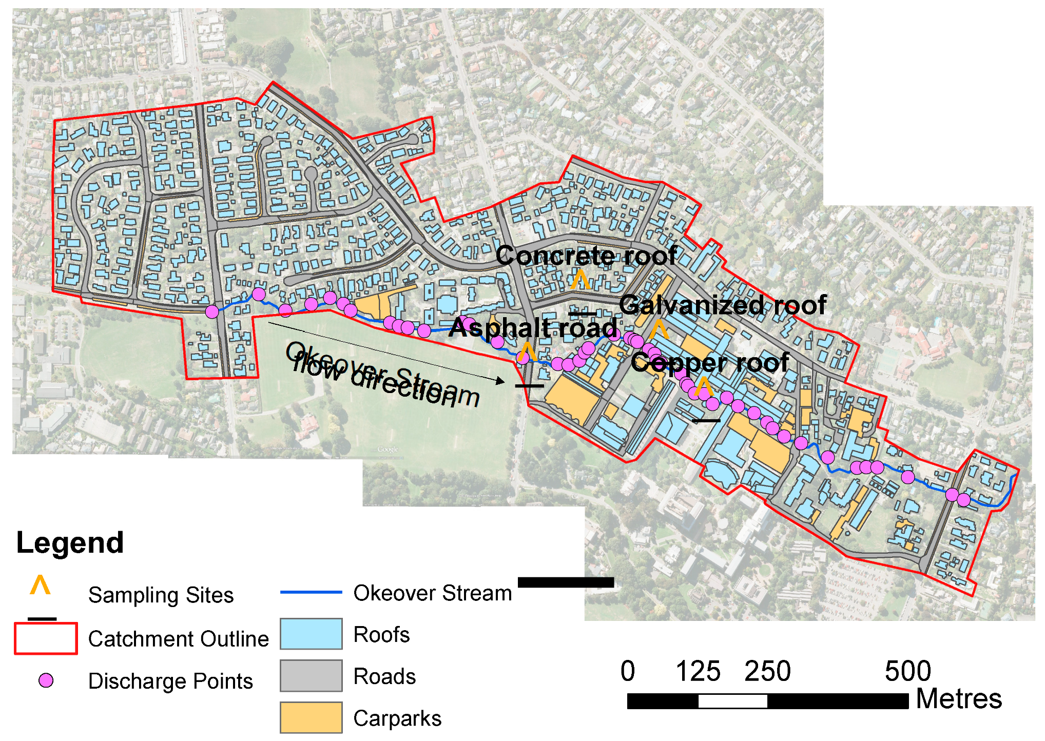
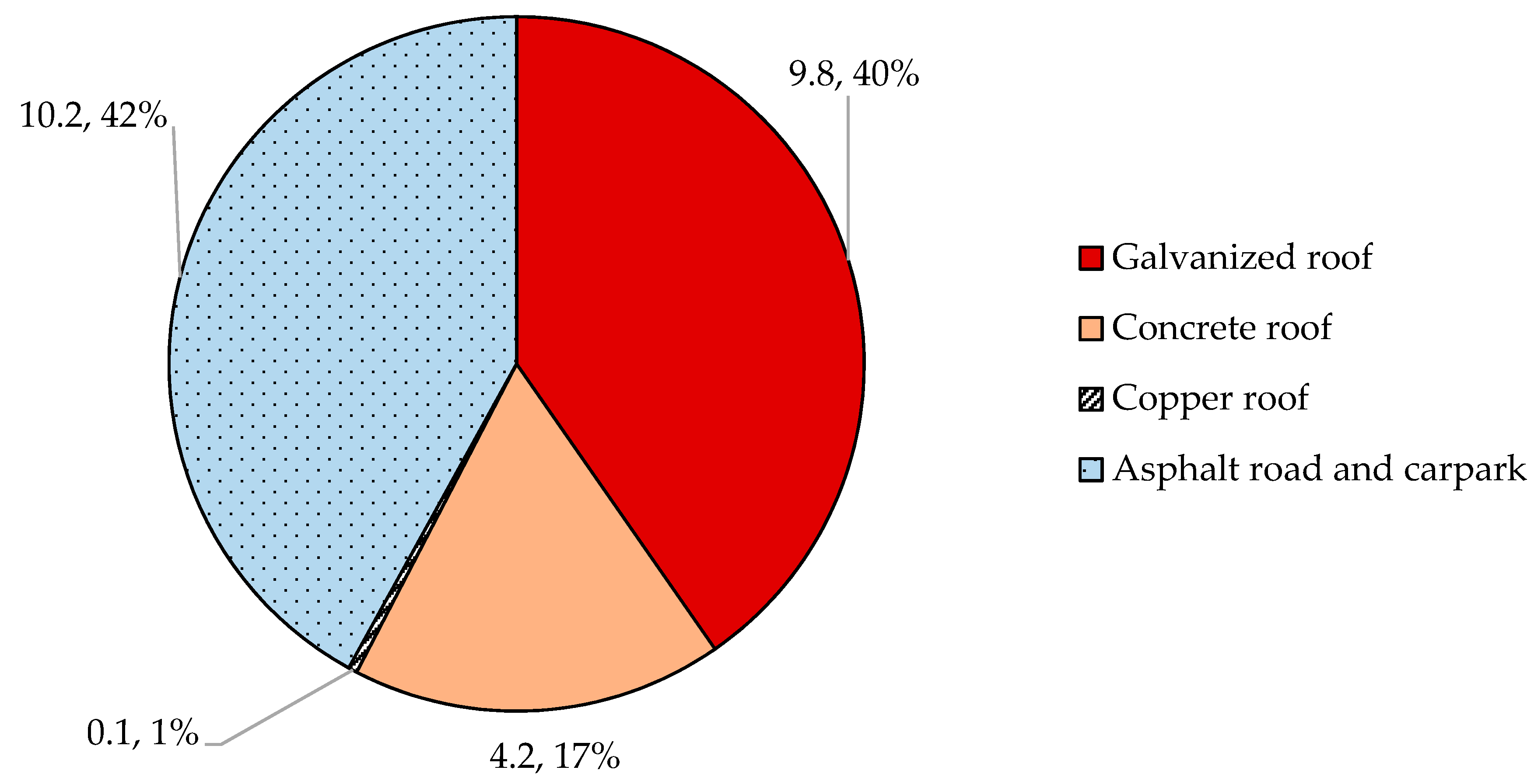
The Okeover Catchment is a mixed residential/institutional catchment in western Christchurch, New Zealand. A GIS map of the 61 ha catchment (of which 40% is impermeable) was developed that delineated all individual roof, road, and carpark surfaces contributing runoff to the stormwater network and ultimately to the Okeover Stream via multiple discharge points (Figure 2). Each surface was classified on the basis of material type and assigned appropriate model properties (Figure 3 and Appendix C). Hardstand areas such as driveways on private residential property were not included in the modelling as their pollutant loads to the net stormwater runoff were considered to be negligible. Roofs are the largest surface type in the catchment (58% of impermeable surfaces), with 51% of roofs galvanized and 25% of roofs concrete tile (Figure 3). MEDUSA2.0 was run for each of the delineated surfaces.
5. Results
5.1. Optimized Model Fits
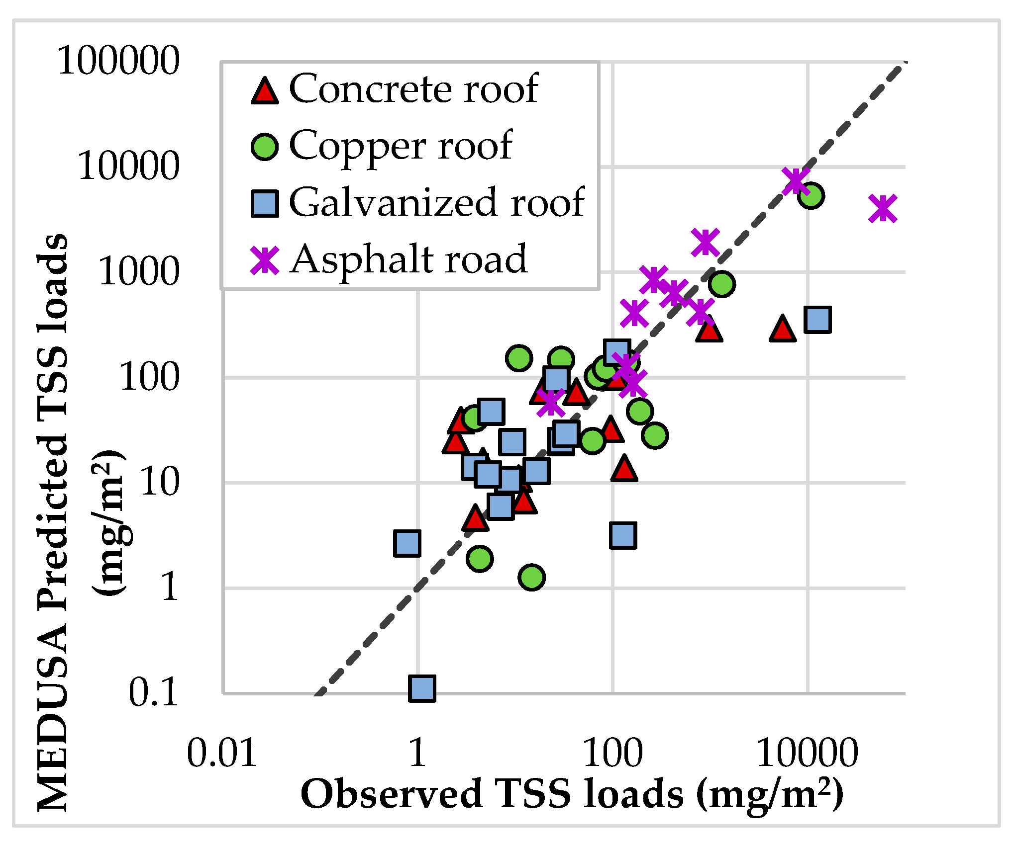
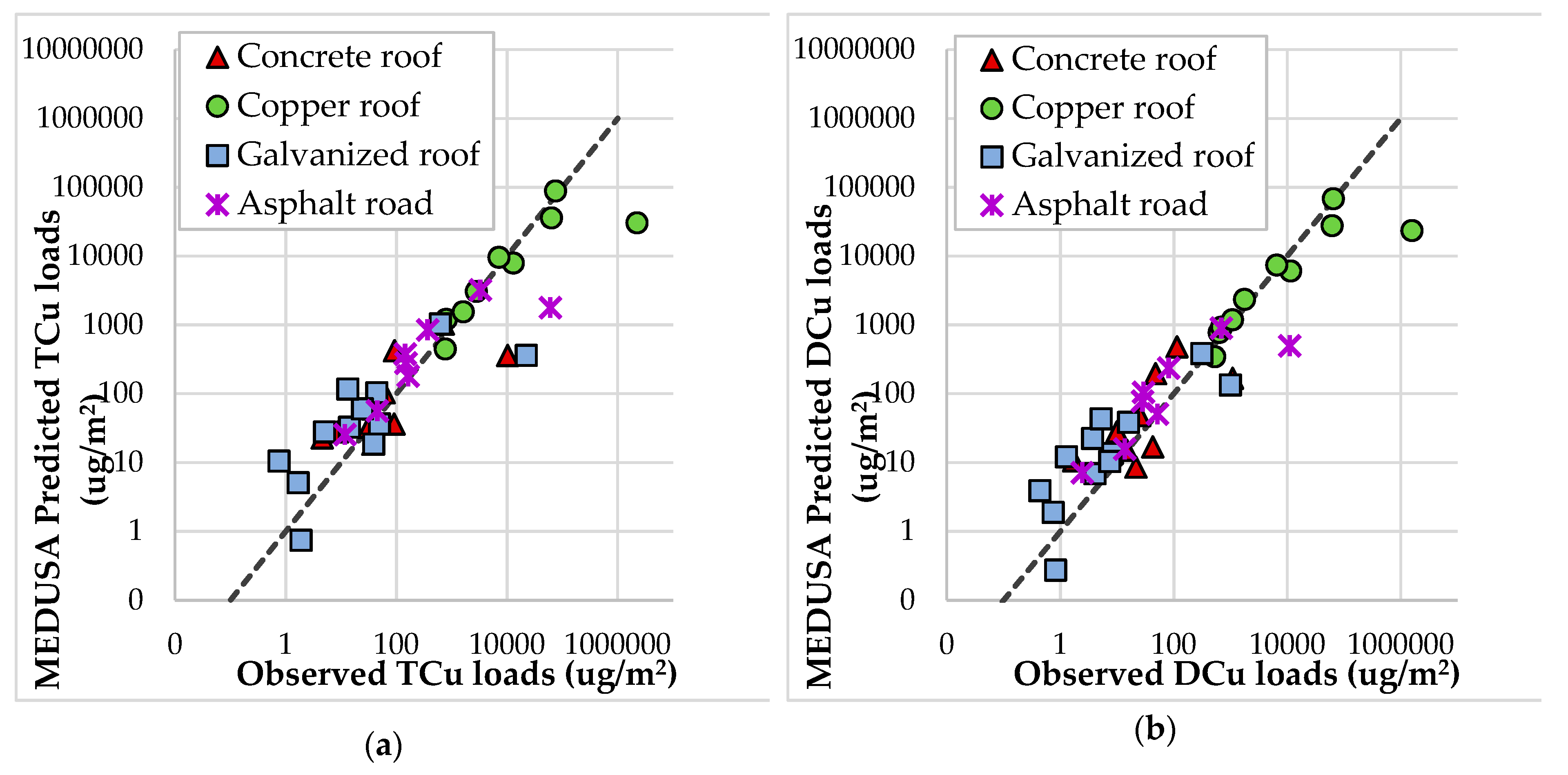
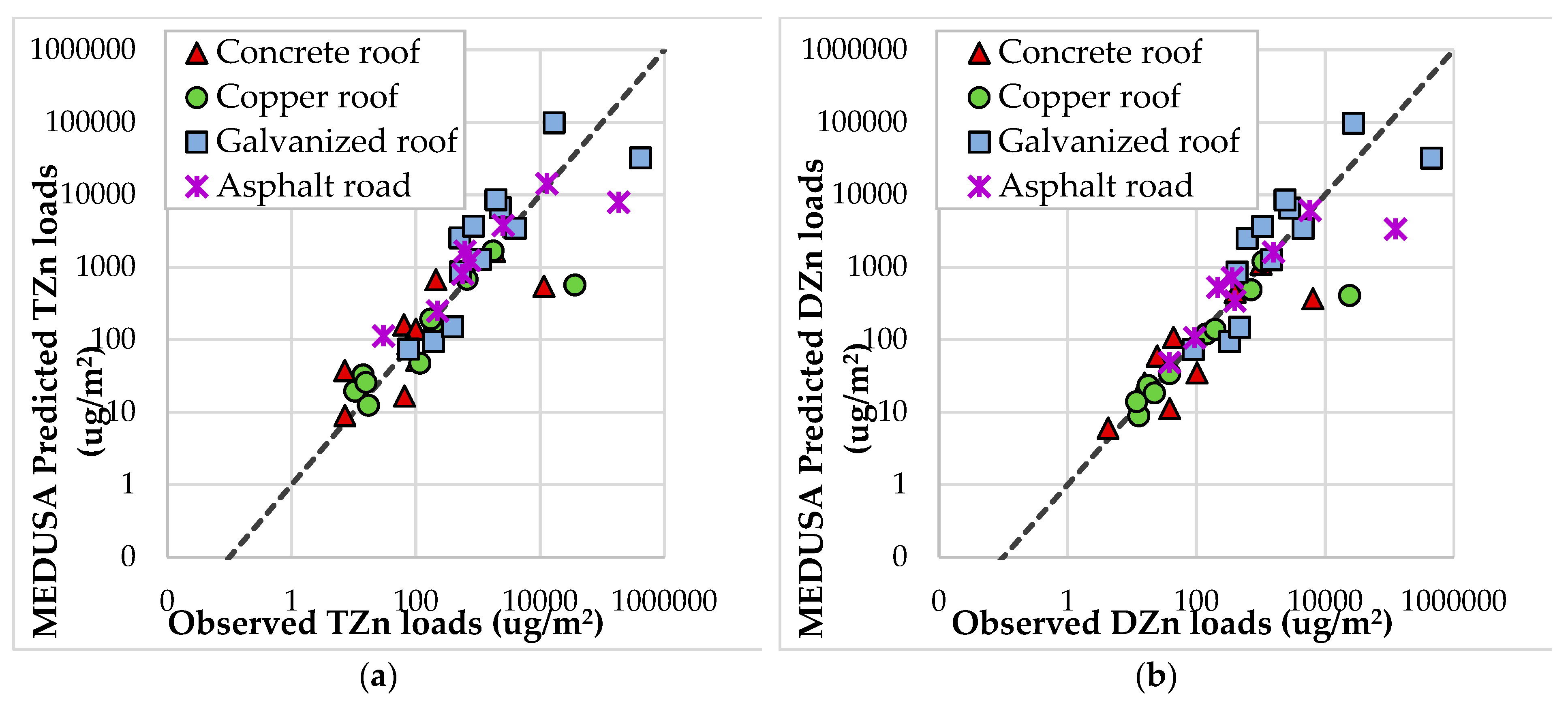
The MEDUSA2.0 model produced moderate to strong goodness of fit NSE values for all pollutants, for all four surfaces (Table 3). Of the four sampled surfaces, the optimized MEDUSA2.0 model was most effective at predicting road runoff pollutant loads (NSEs of 0.66–0.74). The highest copper loads (per area) were from the copper roof, and the model was moderately effective at predicting TCu and DCu from a copper roof (NSEs of 0.46 and 0.69, respectively). The highest zinc loads (per area) were from the galvanized roof, and MEDUSA2.0 was also effective at predicting TZn and DZn from this roof type (NSEs of 0.66 and 0.68, respectively). PBIAS results (see Appendix D) were all < ±10 for the MEDUSA2.0 model, with exceptions of the galvanized roof TCu and DCu models and the copper roof DZn model. The resultant model loads are shown against the observed loads in Figure 4, Figure 5 and Figure 6.
MEDUSA2.0 produced moderate to strong NSEs when applied to untreated runoff data from the same surface types in the adjacent Heathcote catchment used for validation (Table 3), with the sole exception being total and dissolved copper prediction for the galvanised roof. It should be noted that the copper concentrations on the sampled galvanized roofs were found to be low, as the sole source was atmospheric deposition.
5.2. Example Application of MEDUSA2.0 to A Case Study Catchment: Okeover Catchment, Christchurch, New Zealand
Once the model was calibrated and its goodness of fit assessed, the calibrated MEDUSA2.0 model was applied to the local Okeover catchment, where the untreated runoff samples used for model calibration had been collected. The model was run for a full year of rain events from the year 2012 (see Appendix E for summarized event details), as researchers at the University of Canterbury had measured rainfall pH for several rain events in 2012. Therefore, a complete set of characterized rainfall events was available, with minimal assumptions required for rainfall pH. Although there will be variation from year to year, 2012 also had relatively typical annual rainfall for Christchurch (Christchurch Botanic Gardens weather station recorded 631 mm annual rainfall for 2012 [41]); Christchurch’s mean annual rainfall is 647 mm [42] and it provides an indication of the expected variation of rain events across a year. Average event loads were derived from the average of all 88 rain events of 2012.
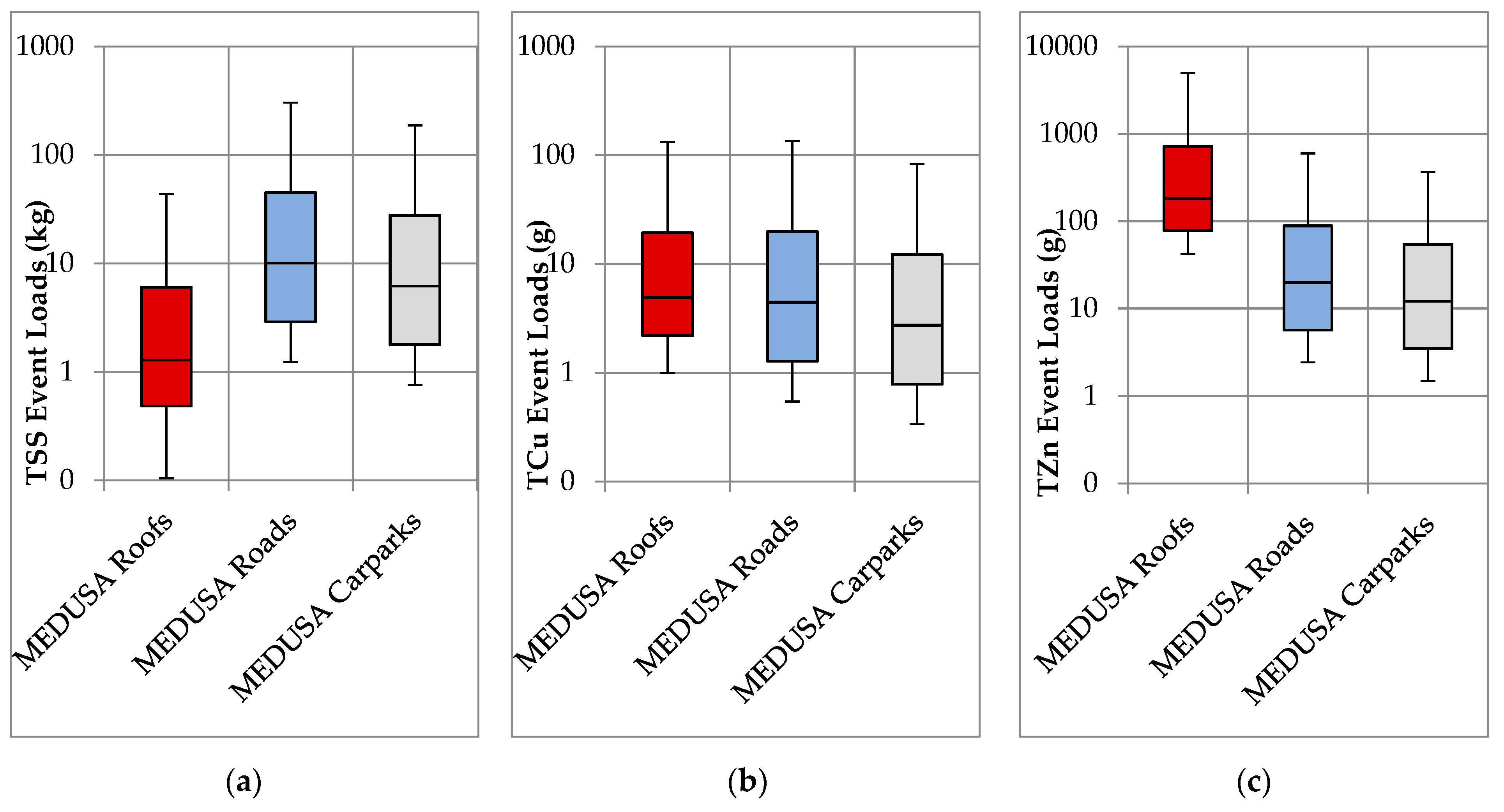
The modelling predicted substantial annual pollutant loads (Table 4), with roads and carparks contributing most of the predicted 4.9 t/year of TSS, but roofs contributing most of the predicted 54 kg/year of zinc. There was also significant load variation (multiple orders of magnitude) for each pollutant across the 88 modelled events (Figure 7).
6. Discussion
6.1. MEDUSA2.0 Model Performance
MEDUSA2.0’s predictive performance was good for all the modelled pollutants with NSE of ≥0.43 for TSS, ≥0.46 for TCu, and ≥0.63 for TZn. MEDUSA2.0 offers a process model that can be calibrated to a particular catchment using local runoff quality data, for estimating pollutant loads from individual impermeable surfaces during each rain event. Where MEDUSA2.0 was able to be applied to surfaces outside the Okeover catchment (i.e., with the Heathcote catchment data), the model produced moderate to strong NSEs with the sole exception of copper loads from the painted galvanised roof. However, as the only source of copper on such a roof is from atmospheric deposition and is of low magnitude, it is not surprising that an effective model fit cannot be readily found. A mean value could instead be derived from local runoff data and applied instead of directly modelling the copper load on such a low-copper surface using rainfall characteristics.
6.2. Influence of Rainfall Characteristics on Pollutant Loads
In the MEDUSA2.0 model, ADD is used to predict TSS loads, regardless of surface type, which is based on observations of dry weather pollutant build-up on surfaces [1,43]. The MEDUSA2.0 model also assumes rainfall pH is a significant variable relating to both initial and second stage copper concentrations, and the initial concentrations are also dependent on ADD and average intensity. For the TCu model, the copper roof was substantially more influenced by rainfall pH than the other two roof surfaces and, to a lesser extent, by average rainfall intensity (see Appendix D for coefficient values). For the TZn model, the galvanized roof was more influenced by rainfall pH (particularly during second stage conditions) than the other two roof surfaces. It was also more influenced by ADD and, to a lesser extent, average rainfall intensity. This could be expected, as the natural (slight) acidity of rainfall is a key driver of the copper and zinc generation (via dissolution) on the copper and galvanized roofs, respectively. Likewise, the influence of ADD could be expected as the dry weather period allows build-up of pollutants from atmospheric deposition, but also, importantly, contributes to weathering and degradation of the metallic surfaces with a corresponding increased leaching rate.
Gnecco et al. [11] did not find any correlation between runoff pollutant amounts such as event mean concentration (EMC) and ADD, and attributed this to the low-to-medium rainfall intensity and low total rainfall volume of their sampled events, where the amount of pollutant wash-off was too low to show differences in dry weather TSS build-up between each event. This study’s rainfall is similarly of low intensity. A study within the same Okeover catchment of atmospherically deposited TSS, copper, and zinc did show that pollutant build-up was significantly influenced by ADD; however, pollutant wash-off processes had a stronger influence than build-up processes on the overall pollutant loads generated from atmospheric deposition [18].
6.3. Individual Model Limitations
Currently, MEDUSA2.0 has a restricted number of pollutant–rainfall parameter relationships, which may inadvertently present inaccurate model coefficient values. For example, the calibrated TSS coefficient values for MEDUSA2.0 suggests that the copper roof was substantially more influenced by ADD than the concrete and galvanised roofs (i.e., higher ADD coefficient values; see Appendix D). However, because MEDUSA2.0’s framework is restricted to relating TSS loads to ADD only, it is likely that the high TSS loads from copper roofs are not due directly to ADD (patination is largely driven by water, carbon dioxide, and time), but simply a means by which the model can reproduce high TSS loads. Furthermore, the NSE values of the calibrated MEDUSA2.0 model were lower for TSS than for metal predictions, suggesting that factors beyond rainfall characteristics are important drivers of pollutant build-up and wash-off. As always, there is a balance sought in the model framework between achieving a reasonable fit without over-parameterization of the model or creating an overly complex running process. Further research is needed to characterize a wider variety of surface types (such as commercial and industrial carparks and roads of different traffic characteristics) to better represent them in the model and incorporate surface factors such as aspect and slope as appropriate. MEDUSA2.0’s use of generalized build-up and wash-off equations allows the model to be applied to catchments outside of Christchurch’s low intensity rainfall climate, and further studies are presently underway to assess the ease and effectiveness of recalibrating MEDUSA2.0 to other catchments as well as serving as further model validation.
MEDUSA2.0 predicts pollutant loads as they are generated at each surface, and therefore does not account for pollutant changes as runoff is conveyed through the stormwater network or discharged into the receiving waterway. Additionally, the presence of sumps (and other (pre)treatment systems), for example, may induce settling of coarse sediment and associated metals, which are removed from the stormwater runoff.
Within its current scope, MEDUSA2.0 allows stormwater managers to identify individual or aggregated impermeable surfaces that can be targeted for optimized stormwater management. However, further research is needed to incorporate multiple stormwater management options and pollutant transformation processes into the MEDUSA2.0 model framework so that different management strategies can be computed within the modelled scenarios.
6.4. Data Limitations
As the available dataset for MEDUSA2.0 model calibration was limited, the entire Okeover dataset was used for calibration instead of truncating the dataset for calibration and having a small validation dataset (following similar approaches by hydrologic modellers, for example Shrestha et al. (2016) [44]). Limited validation data were then provided from untreated runoff sampling in an adjacent catchment for two of the same surface types sampled and modelled in the Okeover catchment. These showed good model performance for the key pollutants of concern from those particular surface types. Further validation data should now be collected from the same surface types as the model has been calibrated for in different geographical locations to expand the conditions under which the model performance is validated. The significant load variation observed in the modelled results for the Okeover case study application indicate that validation data would be particularly valuable for events with rainfall characteristics that produce high event loads (e.g., long duration rain events).
The sampling dataset (that was used to calibrate the model and apply it to the Okeover catchment) was restricted to the four most common impermeable surface types within the catchment. Therefore, assumptions were made by assigning model coefficient values to all the other surface types present in the catchment (Appendix C). Further untreated runoff water quality data are needed from different surface types, particularly carparks, unpainted galvanised roofs, and new painted Zincalume roofs (e.g., Colorsteel) to enable the calibration of model coefficients for a wider range of surface types.
6.5. Implications of Model Predictions on Management Approaches
The variation in MEDUSA2.0 pollutant loading from individual surfaces confirms that it is necessary to apply pollutant load models at an individual surface scale rather than a catchment or land use scale, as surface type is a key driver of pollutant generation. The variations for each pollutant type, for the same surface, also reinforce the need to use specific relationships for each pollutant and rain event, rather than assuming metal loads are proportional to sediment loads as is done with many current models. Metals in dissolved form were a major contributor to metal loads, and therefore it is important that any pollutant model framework does incorporate dissolved metals predictions, as understanding the proportion of metals in dissolved form influences the treatment system selection and source reduction decisions for most effective pollution management. The predicted load variation across multiple rain events must be considered when selecting and designing pollutant treatment systems to ensure effective sizing and maintenance planning.
7. Conclusions
The improvements made to develop MEDUSA2.0 have resulted in a model that performs well in predicting TSS, total and dissolved copper, and total and dissolved zinc loads generated from individual impermeable urban surfaces, with common rainfall parameters being used as the predictor variables. Moderate to strong NSE goodness of fit values were achieved in most instances.
Quantifying the amount of pollutants contributed by each surface during rain events is necessary for the development and implementation of effective and efficient stormwater management options. Furthermore, adopting a modelling approach to predict pollutant loads derived from different impermeable surfaces offers a more cost-effective and reliable tool for understanding pollutant “hotspots” than can be achieved through water quality sampling alone.
Author Contributions
Conceptualization, F.J.C., T.A.C. and A.D.O.; methodology, F.J.C., T.A.C. and A.D.O.; validation, F.J.C.; formal analysis, F.J.C.; investigation, F.J.C.; resources, T.A.C. and A.D.O.; data curation, F.J.C.; writing—original draft preparation, F.J.C.; writing—review and editing, F.J.C., T.A.C. and A.D.O.; visualization, F.J.C.; supervision, T.A.C. and A.D.O; project administration, F.J.C., T.A.C. and A.D.O.; funding acquisition, F.J.C., T.A.C. and A.D.O. All authors have read and agreed to the published version of the manuscript.
Funding
This research received funding from Christchurch City Council, and Frances Charters received scholarship funding while she undertook research on MEDUSA2.0 development and application from the Waterways Centre for Freshwater Management and University of Canterbury’s Department of Civil and Natural Resources Engineering and Scholarships Office.
Acknowledgments
We would like to thank Peter McGuigan from the University of Canterbury for his technical support in the field and in the lab.
Conflicts of Interest
Christchurch City Council approved the Heathcote sampling sites on the basis of the researchers’ recommendations. The authors declare no other conflict of interest.
Appendix A
Total and Dissolved Metal Relationships from Untreated Runoff Sampling Data
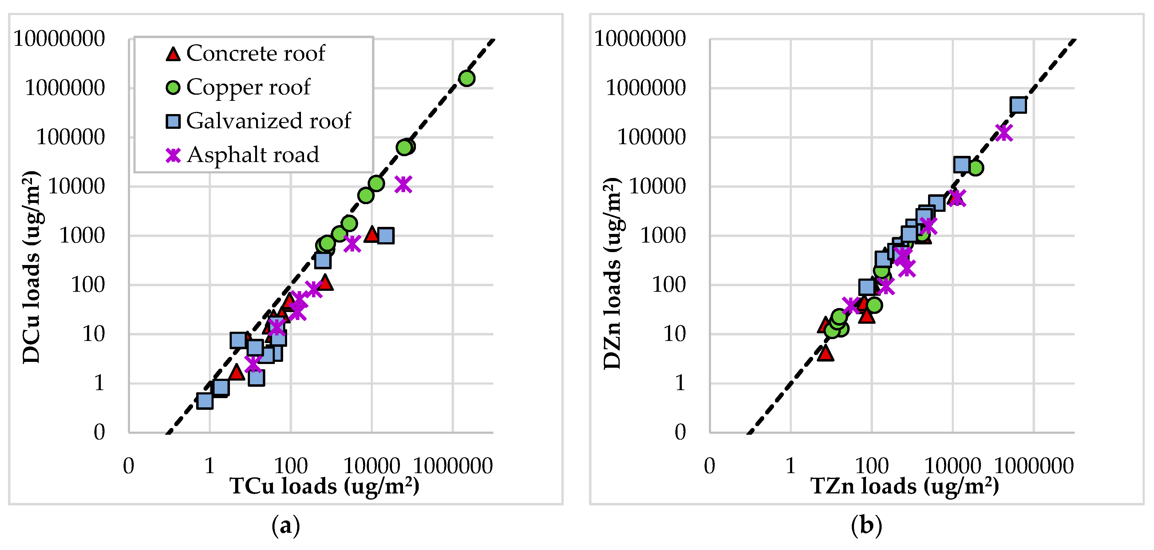
Comparison of observed dissolved loads against total loads for copper and zinc show a strong linear relationship, particularly for the surfaces with the highest loads (Figure A1). This provides a sound basis for the MEDUSA2.0 framework to use a proportional relationship in calculating dissolved metals from total metal loads.
Figure A1.
Relationship between observed dissolved loads and observed total loads for (a) copper and (b) zinc.
Figure A1.
Relationship between observed dissolved loads and observed total loads for (a) copper and (b) zinc.

Appendix B
Summary of Sampled Rainfall Event Characteristics

Table A1.
Okeover sampled event characteristics, used for calibration.
| Event | Date | Rainfall pH | Average Event Intensity (mm/h) | Antecedent Dry Days (days) | Event Duration (h) | Total Rainfall Depth (mm) |
|---|---|---|---|---|---|---|
| 1 | 8 December 2013 | 5.90 | 2.82 | 10.8 | 3.6 | 10.1 |
| 2 | 17 December 2014 | 7.86 | 1.27 | 4.1 | 3.4 | 4.4 |
| 3 | 20 January 2014 | 7.78 | 0.68 | 13.5 | 14.3 | 9.7 |
| 4 | 26 January2014 | 5.78 | 0.46 | 3.1 | 6.4 | 2.9 |
| 5 | 5 February 2014 | 6.46 | 0.80 | 9.3 | 0.3 | 0.2 |
| 6 | 12 February 2014 | 6.35 | 3.41 | 3.6 | 4.0 | 13.6 |
| 7 | 14 February 2014 | 6.33 | 0.20 | 1.1 | 5.1 | 1.0 |
| 8 | 4 March 2014 | 6.35 | 4.61 | 0.6 | 31.3 | 144.2 |
| 9 | 16 March 2014 | 6.38 | 3.00 | 10.5 | 16.3 | 41.2 |
| 10 | 25 March 2014 | 5.58 | 0.20 | 6.1 | 0.1 | 0.2 |
| 11 | 25 March 2014 | 5.58 | 3.20 | 0.2 | 2.9 | 9.2 |
| 12 | 5 April 2014 | 5.98 | 1.47 | 10.7 | 3.6 | 2.2 |
| 13 | 5 May 2014 | 6.01 | 1.60 | 5.6 | 0.3 | 0.4 |
| 14 | 26 May 2014 | 5.86 | 2.40 | 0.6 | 4.9 | 5.2 |
| 15 | 6 June 2014 | 6.26 | 0.30 | 0.3 | 1.3 | 0.4 |
| 16 | 9 June 2014 | 5.82 | 1.37 | 0.2 | 31.4 | 43.0 |
| 17 | 16 June 2014 | 5.46 | 2.40 | 3.9 | 0.3 | 0.8 |
| 18 | 25 June 2014 | 5.81 | 1.48 | 7.3 | 1.1 | 1.6 |
| 19 | 3 October 2014 | 5.74 | 2.03 | 5.4 | 1.1 | 2.2 |
| 20 | 18 October 2014 | 5.10 | 0.56 | 5.4 | 3.6 | 2.0 |
| 21 | 22 November 2014 | 5.67 | 0.53 | 2.8 | 2.4 | 1.3 |
| 22 | 10 December 2014 | 5.93 | 0.80 | 0.2 | 1.3 | 1.0 |
| 23 | 9 February 2015 | 6.31 | 0.90 | 3.6 | 0.7 | 0.6 |
| 24 | 6 March 2015 | 6.05 | 1.41 | 3.2 | 4.3 | 6.0 |
Table A2.
Heathcote sampled event characteristics, used for validation.
| Event | Date | Rainfall pH | Average Event Intensity (mm/h) | Antecedent Dry Days (days) | Event Duration (h) | Total Rainfall Depth (mm) |
|---|---|---|---|---|---|---|
| 1 | 8 July 2016 | 6.29 | 0.81 | 9.66 | 4.0 | 3.2 |
| 2 | 3 August 2016 | 6.60 | 0.16 | 3.23 | 8.8 | 1.4 |
| 3 | 4 August 2016 | 6.02 | 0.43 | 0.71 | 6.8 | 2.9 |
| 4 | 13 August 2016 | 6.64 | 0.49 | 4.24 | 18.0 | 8.8 |
| 5 | 26 August 2016 | 6.79 | 1.76 | 1.29 | 8.0 | 14.0 |
| 6 | 7 September 2016 | 6.53 | 0.79 | 1.45 | 24.8 | 19.5 |
| 7 | 14 October 2016 | 6.74 | 0.47 | 2.01 | 5.8 | 2.7 |
| 8 | 20 October 2016 | 6.17 | 1.70 | 5.60 | 22.3 | 37.8 |
| 9 | 11 November 2016 | -- 1 | 0.40 | 2.22 | 17.5 | 7.0 |
1 Rainfall pH not recorded for Event 9.
Appendix C
Notes:
Calibration data were available for four different surface types: a concrete tile roof (Cr), a copper roof (Cu), a galvanized roof (Gv), and an asphalt road (Rd). Validation data were available for Gv and Rd.
Table A3.
Category allocation for Okeover surface types on the basis of calibrated model coefficients (see Appendix D).
Table A3.
Category allocation for Okeover surface types on the basis of calibrated model coefficients (see Appendix D).
| Surface Type | Modelled Category |
|---|---|
| Galvanised roofs (all age and conditions) | Gv |
| Zincalume and Colorsteel roofs (all age and conditions) | |
| Decramastic tile roofs (all age and conditions) | |
| Copper roofs (all age and conditions) | Cu |
| Concrete roofs | Cr |
| Butynol, glass, fiberglass roofs, and other non-metallic roof materials | |
| Roads (all traffic intensities and surface materials) | Rd |
| Carparks (all usage types and condition) |
Appendix D
Notes:
For Table A4, Table A5, Table A6, Table A7 and Table A8: Cr = concrete tile roof; Cu = copper roof; Gv = galvanized roof; Rd = asphalt road.
See Equations (1) to (11) for coefficient relationships to model variables.
Table A4.
Optimized MEDUSA2.0 model coefficient values and goodness of fit statistics for TZn.
| Surface | TZn Coefficients (Equations (6), (7), and (9)) | NSE | PBIAS | |||||||||
|---|---|---|---|---|---|---|---|---|---|---|---|---|
| b1 | b2 | b3 | b4 | b5 | b6 | b7 | b8 | Z | c1 | |||
| Cr | 50 | 2600 | 0.1 | 0.01 | 1 | −3.1 | −0.007 | 0.056 | 0.75 | 0.632 | −1.71 | |
| Cu | −0.1 | 2 | 0.1 | 0.01 | 0.8 | −1.3 | −0.007 | 0.056 | 0.75 | 0.679 | −7.02 | |
| Gv | 910 | 4 | 0.2 | 0.09 | 1.5 | −2 | −0.23 | 1.990 | 0.75 | 0.657 | 3.97 | |
| Rd | 1.96 | 0.731 | 1.14 | |||||||||
Table A5.
Optimized MEDUSA2.0 model coefficient values and goodness of fit statistics for DZn.
| Surface | DZn Coefficient (Equation (11)) | NSE | PBIAS |
|---|---|---|---|
| d1 | |||
| Cr | 0.67 | 0.69 | −5.2 |
| Cu | 0.72 | 0.68 | −10.6 |
| Gv | 0.43 | 0.68 | 1 |
| Rd | 0.43 | 0.69 | −3.26 |
Table A6.
Optimized MEDUSA2.0 model coefficient values and goodness of fit statistics for TCu.
| Surface | TCu Coefficients (Equations (4), (5), and (8)) | NSE | PBIAS | |||||||||
|---|---|---|---|---|---|---|---|---|---|---|---|---|
| b1 | b2 | b3 | b4 | b5 | b6 | b7 | b8 | Z | c1 | |||
| Cr | 2 | −2.8 | 0.5 | 0.217 | 3.57 | −0.09 | 7 | −3.73 | 0.75 | 0.55 | 1.67 | |
| Cu | 100 | −2.8 | 1.372 | 0.217 | 3.57 | −1 | 275 | −3.3 | 0.75 | 0.68 | −5.09 | |
| Gv | 2 | −2.8 | 0.5 | 0.217 | 3.57 | −0.09 | 7 | −3.73 | 0.75 | 0.58 | 11.47 | |
| Rd | 0.441 | 0.69 | −0.05 | |||||||||
Table A7.
Optimized MEDUSA2.0 model coefficient values and goodness of fit statistics for DCu.
| Surface | DCu Coefficient (Equation (10)) | NSE | PBIAS |
|---|---|---|---|
| d1 | |||
| Cr | 0.46 | 0.47 | 9.4 |
| Cu | 0.77 | 0.69 | −5.8 |
| Gv | 0.28 | 0.59 | 37 |
| Rd | 0.28 | 0.68 | 4.9 |
Table A8.
Optimized MEDUSA2.0 model coefficient values and goodness of fit statistics for TSS.
| Surface | TSS Coefficients (Equation (1)) | NSE | PBIAS | ||
|---|---|---|---|---|---|
| a1 | a2 | a3 | |||
| Cr | 0.6 | 0.25 | 9.33 × 10⁻³ | 0.503 | 0.2 |
| Cu | 2.5 | 0.95 | 9.33 × 10⁻³ | 0.487 | −3.2 |
| Gv | 0.6 | 0.5 | 9.33 × 10⁻³ | 0.430 | −4.5 |
| Rd | 2.9 | 0.16 | 8.0 × 10⁻⁴ | 0.736 | 0.1 |
Appendix E
Table A9.
Summarized rainfall event characteristics for the year 2012.
| Rainfall Parameter | Median Value (Range) |
|---|---|
| Number of rain events | 88 |
| Rainfall pH | 6.01 (5.19–7.15) |
| Average intensity (mm/h) | 0.53 (0.12–4.00) |
| Antecedent dry days (days) | 3.0 (0.2–19.0) |
| Event duration (hours) | 5.0 (1.0–41.0) |
References
- Egodawatta, P.; Thomas, E.; Goonetilleke, A. Understanding the physical processes of pollutant build-up and wash-off on roof surfaces. Sci. Total. Environ. 2009, 407, 1834–1841. [Google Scholar] [CrossRef] [PubMed] [Green Version]
- Wicke, D.; Cochrane, T.; O’Sullivan, A. Build-up dynamics of heavy metals deposited on impermeable urban surfaces. J. Environ. Manag. 2012, 113, 347–354. [Google Scholar] [CrossRef] [PubMed]
- Zanders, J. Road sediment: Characterization and implications for the performance of vegetated strips for treating road run-off. Sci. Total. Environ. 2005, 339, 41–47. [Google Scholar] [CrossRef] [PubMed]
- Sabin, L.D.; Lim, J.H.; Stolzenbach, K.D.; Schiff, K.C. Contribution of trace metals from atmospheric deposition to stormwater runoff in a small impervious urban catchment. Water Res. 2005, 39, 3929–3937. [Google Scholar] [CrossRef] [PubMed]
- Quek, U. Trace metals in roof runoff. Water, Air, Soil Pollut. 1993, 68, 373–389. [Google Scholar] [CrossRef]
- Wicke, D.; Cochrane, T.; O’Sullivan, A.D.; Cave, S.; Derksen, M. Effect of age and rainfall pH on contaminant yields from metal roofs. Water Sci. Technol. 2014, 69, 2166–2173. [Google Scholar] [CrossRef]
- Barrett, M.; Irish, L.B., Jr.; Malina, J.F., Jr.; Charbeneau, R.J. Characterization of Highway Runoff in Austin, Texas, Area. J. Environ. Eng. 1998, 124, 131–137. [Google Scholar] [CrossRef] [Green Version]
- He, W.; Wallinder, I.O.; Leygraf, C. A laboratory study of copper and zinc runoff during first flush and steady-state conditions. Corros. Sci. 2001, 43, 127–146. [Google Scholar] [CrossRef]
- Brezonik, P.L.; Stadelmann, T.H. Analysis and predictive models of stormwater runoff volumes, loads, and pollutant concentrations from watersheds in the Twin Cities metropolitan area, Minnesota, USA. Water Res. 2002, 36, 1743–1757. [Google Scholar] [CrossRef]
- Vaze, J.; Chiew, F.H.S. Study of pollutant washoff from small impervious experimental plots. Water Resour. Res. 2003, 39. [Google Scholar] [CrossRef]
- Gnecco, I.; Berretta, C.; Lanza, L.G.; La Barbera, P. Storm water pollution in the urban environment of Genoa, Italy. Atmos. Res. 2005, 77, 60–73. [Google Scholar] [CrossRef]
- Crabtree, B.; Moy, F.; Whitehead, M.; Roe, A. Monitoring pollutants in highway runoff. Water Environ. J. 2006, 20, 287–294. [Google Scholar] [CrossRef]
- Desta, M.B.; Bruen, M.; Higgins, N.; Johnston, P. Highway runoff quality in Ireland. J. Environ. Monit. 2007, 9, 366. [Google Scholar] [CrossRef] [PubMed]
- Wicke, D.; Cochrane, T.; O’Sullivan, A.; Hutchinson, J.; Funnell, E. Developing a Rainfall Contaminant Relationship Model for Christchurch Urban Catchments. In Proceedings of the Water New Zealand’s 6th South Pacific Stormwater Conference, Auckland, New Zealand, April 2009. [Google Scholar]
- Brodie, I.; Dunn, P.K. Commonality of rainfall variables influencing suspended solids concentrations in storm runoff from three different urban impervious surfaces. J. Hydrol. 2010, 387, 202–211. [Google Scholar] [CrossRef] [Green Version]
- Brodie, I.; Egodawatta, P. Relationships between rainfall intensity, duration and suspended particle washoff from an urban road surface. Hydrol. Res. 2011, 42, 239–249. [Google Scholar] [CrossRef] [Green Version]
- Gunawardena, J.; Egodawatta, P.; Ayoko, G.A.; Goonetilleke, A. Atmospheric deposition as a source of heavy metals in urban stormwater. Atmos. Environ. 2013, 68, 235–242. [Google Scholar] [CrossRef] [Green Version]
- Murphy, L.U.; Cochrane, T.; O’Sullivan, A. Build-up and wash-off dynamics of atmospherically derived Cu, Pb, Zn and TSS in stormwater runoff as a function of meteorological characteristics. Sci. Total. Environ. 2015, 508, 206–213. [Google Scholar] [CrossRef]
- Cheema, P.P.S.; Reddy, A.S.; Kaur, S. Characterization and prediction of stormwater runoff quality in sub-tropical rural catchments. Water Resour. 2017, 44, 331–341. [Google Scholar] [CrossRef]
- Salim, I.; Paule-Mercado, M.C.; Sajjad, R.U.; Memon, S.A.; Lee, B.-Y.; Sukhbaatar, C. Trend analysis of rainfall characteristics and its impact on stormwater runoff quality from urban and agricultural catchment. Membr. Water Treat. 2019, 10, 45–55. [Google Scholar]
- Bąk, Ł.; Szeląg, B.; Górski, J.; Górska, K. The Impact of Catchment Characteristics and Weather Conditions on Heavy Metal Concentrations in Stormwater—Data Mining Approach. Appl. Sci. 2019, 9, 2210. [Google Scholar] [CrossRef] [Green Version]
- Poudyal, D.S. Characterizing Stormwater Pollutant Yields from Urban Carparks in a Low-Intensity Rainfall Climate; University of Canterbury: Christchurch, New Zealand, 2019. [Google Scholar]
- Charbeneau, R.J.; Barrett, M.E. Evaluation of methods for estimating stormwater pollutant loads. Water Environ. Res. 1998, 70, 1295–1302. [Google Scholar] [CrossRef]
- Egodawatta, P.; Thomas, E.; Goonetilleke, A. Mathematical interpretation of pollutant wash-off from urban road surfaces using simulated rainfall. Water Res. 2007, 41, 3025–3031. [Google Scholar] [CrossRef] [PubMed] [Green Version]
- Deletic, A.; Maksimovic, C.E.; Ivetic, M. Modelling of storm wash-off of suspended solids from impervious surfaces. J. Hydraul. Res. 1997, 35, 99–118. [Google Scholar] [CrossRef]
- Zoppou, C. Review of urban storm water models. Environ. Model. Softw. 2001, 16, 195–231. [Google Scholar] [CrossRef]
- Auckland Regional Council. Development of the Contaminant Load Model; Auckland Regional Council: Auckland, New Zealand, 2010. [Google Scholar]
- James, W.; Boregowda, S. Continuous Mass-Balance of Pollutant Build-Up Processes; Springer Science and Business Media: Berlin, Germany, 1986; pp. 243–271. [Google Scholar]
- Fraga, I.; Charters, F.; O’Sullivan, A.; Cochrane, T. A novel modelling framework to prioritize estimation of non-point source pollution parameters for quantifying pollutant origin and discharge in urban catchments. J. Environ. Manag. 2016, 167, 75–84. [Google Scholar] [CrossRef]
- Sartor, J.D.; Boyd, G.B.; Agardy, F.J. Water pollution aspects of street surface contaminants. J. Water Pollut. Control. Fed. 1974, 46. [Google Scholar]
- Margetts, B. Wet Weather Monitoring Report for the Period May 2013–April 2014; Christchurch City Council: Christchurch, New Zealand, 2014. [Google Scholar]
- Margetts, B.; Marshall, W. Wet Weather Monitoring Report for the Period 14–April 2015; Christchurch City Council: Christchurch, New Zealand, 2015. [Google Scholar]
- Clark, S.E.; Steele, K.A.; Spicher, J.; Siu, C.Y.; Lalor, M.M.; Pitt, R.E.; Kirby, J.T. Roofing Materials’ Contributions to Storm-Water Runoff Pollution. J. Irrig. Drain. Eng. 2008, 134, 638–645. [Google Scholar] [CrossRef] [Green Version]
- Förstner, U.; Wittmann, G.T. Metal Pollution in the Aquatic Environment; Springer Science & Business Media: Berlin, Germany, 2012. [Google Scholar]
- Chui, P. Characteristics of Stormwater Quality from Two Urban Watersheds in Singapore. Environ. Monit. Assess. 1997, 44, 173–181. [Google Scholar] [CrossRef]
- Charters, F.; Cochrane, T.; O’Sullivan, A.D. Particle size distribution variance in untreated urban runoff and its implication on treatment selection. Water Res. 2015, 85, 337–345. [Google Scholar] [CrossRef]
- Nash, J.E.; Sutcliffe, J.V. River Flow forecasting through conceptual models-Part I: A discussion of principles. J. Hydrol. 1970, 10, 282–290. [Google Scholar] [CrossRef]
- Moriasi, D.N.; Arnold, J.G.; Van Liew, M.W.; Bingner, R.L.; Harmel, R.D.; Veith, T.L. Model Evaluation Guidelines for Systematic Quantification of Accuracy in Watershed Simulations. Trans. ASABE 2007, 50, 885–900. [Google Scholar] [CrossRef]
- Krause, P.; Boyle, D.P.; Bäse, F. Comparison of different efficiency criteria for hydrological model assessment. Adv. Geosci. 2005, 5, 89–97. [Google Scholar] [CrossRef] [Green Version]
- Gupta, H.; Sorooshian, S.; Yapo, P.O. Status of Automatic Calibration for Hydrologic Models: Comparison with Multilevel Expert Calibration. J. Hydrol. Eng. 1999, 4, 135–143. [Google Scholar] [CrossRef]
- NIWA. Errata and Updated Statistics for the 2012 Annual Climate Summary. Available online: https://www.niwa.co.nz/sites/niwa.co.nz/files/updated_annual_summary_2012_final.pdf2013 (accessed on 21 January 2020).
- NIWA. Climate Summaries. Available online: https://www.niwa.co.nz/education-and-training/schools/resources/climate/summary2013 (accessed on 21 January 2020).
- Charters, F.; Cochrane, T.; O’Sullivan, A.D. Untreated runoff quality from roof and road surfaces in a low intensity rainfall climate. Sci. Total. Environ. 2016, 550, 265–272. [Google Scholar] [CrossRef] [PubMed]
- Shrestha, B.; Cochrane, T.; Caruso, B.S.; E Arias, M.; Piman, T. Uncertainty in flow and sediment projections due to future climate scenarios for the 3S Rivers in the Mekong Basin. J. Hydrol. 2016, 540, 1088–1104. [Google Scholar] [CrossRef]
Figure 1.
MEDUSA2.0 model framework. TSS, total suspended solids; TCu, total copper; DCu, dissolved copper; TZn, total zinc; DZn, dissolved zinc.
Figure 1.
MEDUSA2.0 model framework. TSS, total suspended solids; TCu, total copper; DCu, dissolved copper; TZn, total zinc; DZn, dissolved zinc.

Figure 2.
Map of impermeable surfaces and stormwater sampling sites in the Okeover Catchment, Christchurch, New Zealand.
Figure 2.
Map of impermeable surfaces and stormwater sampling sites in the Okeover Catchment, Christchurch, New Zealand.

Figure 3.
Relative impermeable area (ha) and percentage of surface type.

Figure 4.
Predicted total suspended solids (TSS) loads against observed loads for Okeover surfaces.

Figure 5.
Predicted loads against observed loads for (a) total copper and (b) dissolved copper, for Okeover surfaces.
Figure 5.
Predicted loads against observed loads for (a) total copper and (b) dissolved copper, for Okeover surfaces.

Figure 6.
Predicted loads against observed loads for (a) total zinc and (b) dissolved zinc, for Okeover surfaces.
Figure 6.
Predicted loads against observed loads for (a) total zinc and (b) dissolved zinc, for Okeover surfaces.

Figure 7.
Event load variation across the 88 modelled events of 2012, by surface type, for (a) TSS, (b) total copper, and (c) total zinc.
Figure 7.
Event load variation across the 88 modelled events of 2012, by surface type, for (a) TSS, (b) total copper, and (c) total zinc.

Table 1.
Reported relationships between pollutants in untreated runoff and rainfall characteristics (chronological order).
Table 1.
Reported relationships between pollutants in untreated runoff and rainfall characteristics (chronological order).
| Runoff Type | Year of Study | TSS | Total Copper and Zinc |
|---|---|---|---|
| Highway | 1998 [7] | INTavg, runoff volume | |
| Roof (copper) | 2001 [8] | Cu only: INTavg (power relationship) | |
| Urban runoff | 2002 [9] | Dur, INTavg, days since last event >25 mm | |
| Urban runoff | 2003 [10] | Rainfall intensity | |
| Roof, road | 2005 [11] | Significant: INTpeak; Not significant: ADD, INTavg, Depth, Runoff volume, Max runoff discharge | |
| Highway | 2006 [12] | Depth, INTpeak | |
| Highway | 2007 [13] | Significant: INTavg; Not significant: ADD, Depth, Dur, Runoff volume | |
| Carpark | 2009 [14] | ADD | ADD |
| Carpark, roof, road | 2010 [15] | Most significant: Depth, INTpeak, Less so: Dur, antecedent storm rainfall depth | |
| Urban street | 2011 [16] | INTavg, INTpeak, Dur | |
| Atmospheric deposition | 2013 [17] | Dry deposition: ADD; Bulk deposition: Depth | |
| Roof (copper, galvanized) | 2014 [6] | pH (Cu: power relationship; Zn: linear relationship) | |
| Atmospheric deposition | 2015 [18] | INTpeak, Dur | Depth |
| Urban runoff | 2017 [19] | ADD, Depth | ADD Zn only - Not significant: Depth |
| Urban runoff | 2019 [20] | Significant: ADD, Depth, INTavg | |
| Urban runoff | 2019 [21] | Significant: Depth, INTpeak, ADD (all negative correlations) Not significant: Dur | |
| Carpark | 2019 [22] | Depth, ADD | Depth, ADD |
Note: TSS, total suspended solids; ADD, antecedent dry days; Dur, duration; INTavg, average intensity; INTpeak, peak intensity.
Table 2.
Rainfall characteristics used in the urban runoff pollutant load modelling.
| Rainfall Characteristic | Significance in Pollutant Generation Processes |
|---|---|
| Rainfall pH | Rainfall is naturally acidic due to raindrops’ scavenging of carbon dioxide to form carbonic acid as they fall. The low pH can dissolve metallic components of a surface [33,34]. |
| Rainfall intensity (mm/h) | Average event intensity was characterized for each sampled event. The intensity is an indication of the kinetic energy present that allows the entrainment and transport of particles in runoff from a surface [24]. |
| Length of antecedent dry period (days) | Pollutants accumulate on impermeable surfaces due to atmospheric deposition, direct deposition from vehicles, and weathering of surface, during the dry periods between rain events. Studies have shown a log or arctan relationship where pollutant build-up rates are most rapid at the start of the antecedent dry period then slower over time [6]. |
| Event duration (h) | Pollutant wash-off continues throughout a rain event, however, the rate of wash-off is generally expected to reduce (exponentially) over the course of a rain event due to the decreasing amount of available material remaining on the surface [23]. |
| Depth of event (mm) | Greater rainfall depths, and therefore larger rainfall volumes, will generate larger total amounts of pollutants [35]. |
Table 3.
Nash–Sutcliffe model efficiencies (NSEs) of MEDUSA2.0 predicted loads against observed loads for the Okeover surfaces (calibration) and Heathcote surfaces (validation).
Table 3.
Nash–Sutcliffe model efficiencies (NSEs) of MEDUSA2.0 predicted loads against observed loads for the Okeover surfaces (calibration) and Heathcote surfaces (validation).
| Parameter | Surface | Okeover Surfaces | Heathcote Surfaces |
|---|---|---|---|
| TSS | Concrete roof | 0.50 | |
| Copper roof | 0.49 | ||
| Galvanized roof | 0.43 | 0.63 | |
| Asphalt road | 0.74 | 0.75 | |
| TCu | Concrete roof | 0.55 | |
| Copper roof | 0.46 | ||
| Galvanized roof | 0.58 | 0.18 | |
| Asphalt road | 0.66 | 0.71 | |
| DCu | Concrete roof | 0.47 | |
| Copper roof | 0.69 | ||
| Galvanized roof | 0.59 | −0.72 | |
| Asphalt road | 0.68 | 0.69 | |
| TZn | Concrete roof | 0.63 | |
| Copper roof | 0.68 | ||
| Galvanized roof | 0.66 | 0.56 | |
| Asphalt road | 0.73 | 0.72 | |
| DZn | Concrete roof | 0.69 | |
| Copper roof | 0.68 | ||
| Galvanized roof | 0.68 | 0.71 | |
| Asphalt road | 0.69 | 0.80 |
Note: TSS, total suspended solids; TCu, total copper; DCu, dissolved copper; TZn, total zinc; DZn, dissolved zinc.
Table 4.
Predicted total annual pollutant loads in Okeover catchment.
| Surface Type | TSS (kg/year) | TCu (kg/year) | TZn (kg/year) |
|---|---|---|---|
| Roofs | 439 | 1.2 | 45.3 |
| Roads | 2770 | 1.2 | 5.4 |
| Carparks | 1704 | 0.8 | 3.3 |
| Total | 4914 | 3.2 | 54.1 |
© 2020 by the authors. Licensee MDPI, Basel, Switzerland. This article is an open access article distributed under the terms and conditions of the Creative Commons Attribution (CC BY) license (http://creativecommons.org/licenses/by/4.0/).
Share and Cite
MDPI and ACS Style
Charters, F.J.; Cochrane, T.A.; O’Sullivan, A.D. Predicting Event-Based Sediment and Heavy Metal Loads in Untreated Urban Runoff from Impermeable Surfaces. Water 2020, 12, 969. https://doi.org/10.3390/w12040969
AMA Style
Charters FJ, Cochrane TA, O’Sullivan AD. Predicting Event-Based Sediment and Heavy Metal Loads in Untreated Urban Runoff from Impermeable Surfaces. Water. 2020; 12(4):969. https://doi.org/10.3390/w12040969
Chicago/Turabian StyleCharters, Frances J., Thomas A. Cochrane, and Aisling D. O’Sullivan. 2020. "Predicting Event-Based Sediment and Heavy Metal Loads in Untreated Urban Runoff from Impermeable Surfaces" Water 12, no. 4: 969. https://doi.org/10.3390/w12040969
Note that from the first issue of 2016, this journal uses article numbers instead of page numbers. See further details here.