Comparative Analysis of Water Quality Disparities in the United States in Relation to Heavy Metals and Biological Contaminants


1
Department of Chemistry, Tennessee State University, Nashville, TN 37209, USA
2
Department of Biological Sciences, Tennessee State University, Nashville, TN 37209, USA
*
Author to whom correspondence should be addressed.
Water 2020, 12(4), 967; https://doi.org/10.3390/w12040967
Submission received: 27 February 2020
/
Revised: 26 March 2020
/
Accepted: 26 March 2020
/
Published: 29 March 2020
(This article belongs to the Section Water Resources Management, Policy and Governance)
Abstract
:Drinking water quality can be compromised by heavy metals, such as copper and lead. If consumed raw, water can pose a health burden to the general population. In this study, the roles of heavy metals and biological contaminants have been explored in determining the quality of drinking water available to consumers of various socioeconomic backgrounds in the United States. In an effort to gain an understanding of possible social disparities in drinking water, a quantitative analysis was conducted to examine whether vulnerable populations are disproportionately impacted by drinking water contaminants. Our data indicated that states with middle-average household incomes were statistically more susceptible to higher levels of lead in drinking water. The states with higher-average household incomes demonstrated lower copper levels compared to those with lower incomes, although a direct correlation was not present. No statistical significance was observed in the total coliform and turbidity levels in correlation to the average household incomes. In general, more violations in water quality were prevalent in middle-income states when compared to the states with lower-average household incomes.
1. Introduction
Drinking water is a for-granted utility for many people in the United States. It is obtained from ground and surface sources, prior to being treated with chemicals to meet federal standards. If consumed raw, water can pose a health burden to the general population. Although 92% of water in the United States is believed to meet the Environmental Protection Agency (EPA) standards [1], 8% of the drinking water produced by water treatment facilities does not adhere to these safety standards. Considering private wells are not regulated by the federal government, about forty million individuals in the United States [2] are left uncovered by the Safe Drinking Water Act [3]. This inadequacy in the justice system leaves hundreds of small and rural communities vulnerable to unsafe drinking water, due to modest socioeconomic backgrounds dictating their inability to mitigate the risks.
There is a considerably large population that lacks the means to obtain clean drinking water in rural areas, as their water sources can become contaminated by runoff from livestock and agricultural waste and by chemical by-products [4]. Regulated city water, on the other hand, can have elevated levels of heavy metal, among other contaminants, as shown in a case study conducted for different counties in the State of Tennessee [5]. Heavy metals, such as copper and lead, are among some of the chemicals regulated by the EPA due to their adverse effects on the development and cognition of children. The EPA requires lead and copper levels in drinking water to remain below 15 parts per billion and below 1.3 parts per million, respectively [6]. Studies have shown that even low levels of lead can burden the body, impair normal cognitive function in children, and lead to behavioral and learning disorders [7,8,9].
In addition to heavy metals, numerous microorganisms, including those found in fecal matter such as Campylobacter ssp., Cryptosporidium parvum, rotavirus, and Legionella ssp. [10], can be found in drinking water sources. Pathogens such as Cryptosporidium, Giardia lamblia, Legionella, and total coliform, which include fecal coliform and E. coli, can cause illnesses among humans if ingested [11]. Total coliform can also be found in regulated water and is known to cause diseases among the general population, especially among children, pregnant women, and immunocompromised individuals [12,13,14]. Turbidity, the main source of physical contaminants in raw water, is the measure of water cloudiness and is attributed to the presence of invisible particles, due to agriculture, mining, and storm water runoff. Higher turbidity levels are often associated with higher levels of disease-causing microorganisms such as viruses, parasites, and some bacteria [6]. The World Health Organization (WHO) and the EPA recommend that turbidity remains below 5 Nephelometric Turbidity Units, (NTU) [15,16].
Differences in water quality have been shown to impact unregulated water in rural areas, due to inadequate services and infrastructure [17]. Social disparities are persistent in drinking water, as shown in a study where arsenic and nitrate contaminants were correlated to race/ethnicity and socioeconomic backgrounds [18,19]. To understand the social disparities, it is important to conduct a quantitative analysis to examine whether vulnerable populations, especially those with lower-average household incomes, are disproportionately impacted by drinking water contaminants. This research aims to explore where the disparities exist in drinking water quality and their correlation to the socioeconomic backgrounds of the consumers.
2. Materials and Methods
Secondary water quality data were collected for the metropolitan areas (city water department) for each state in 2019. Additional data not published on the yearly water safety report were obtained from each city’s water supply office. To ensure bias-free results, data were obtained from three of the most populated counties in each state, including the state capitals. The data were supplied by each city’s water service department. The water sources for each state differs, and a majority of the raw water was obtained from groundwater or surface water sources. The primary surface water sources corresponding to the metropolitan areas of each state are listed in Table 1.
The average household income data were obtained from the United States Census Bureau, which was last published in 2018 [20]. Raw data were initially tested and further analyzed by the Statistical Analysis System (SAS) software (SAS Institute, Cary, NC, USA) at type 1 error level utilizing the analysis of variance (ANOVA) test. Tukey’s grouping test was utilized to determine the variation among different income brackets for the level of contaminants in drinking water. Statistically significant variations, obtained from Tukey’s test, were denoted by an asterisk (*). The samples were sub-grouped into $10,000 intervals for average household income groups. The corresponding contaminant levels were obtained for each income group and the data were numerically analyzed. To compare the contaminant levels among different income groups, Tukey’s test was utilized to examine statistical significance among different means [21]. Histograms were utilized to plot the levels of lead, copper, total coliform, and turbidity in the different states, corresponding to the average household income. This enabled the investigation of possible correlation between the levels of the heavy metals (lead, copper) and biological contaminants (total coliform, turbidity) to the average household income. Multivariable charts were employed to demonstrate disparities in water quality as it correlates to the household income in each state. In addition, a scatter plot was utilized to examine the spread of lead data corresponding to each state, as related to the average household income.
3. Results and Discussion
Figure 1, Figure 2, Figure 3 and Figure 4 show the correlation between the average household income and levels of copper, lead, total coliform, and turbidity, respectively, for various states. To examine the impact of income on the quality of drinking water, data were obtained from the metropolitan public water systems of each state. The drinking water sources in each state are different; however, the majority of the water sources are either from surface water or groundwater. The primary sources of surface water have been listed in Table 1 under the Materials and Methods. The data were limited to the metropolitan cities of each state. Rural areas were omitted to ensure that all data were governed by similar parameters in order to avoid bias. In this manner, the data obtained were carefully controlled for any bias or discrepancy that would have arisen if unregulated water sources (from rural areas) were to be evaluated.
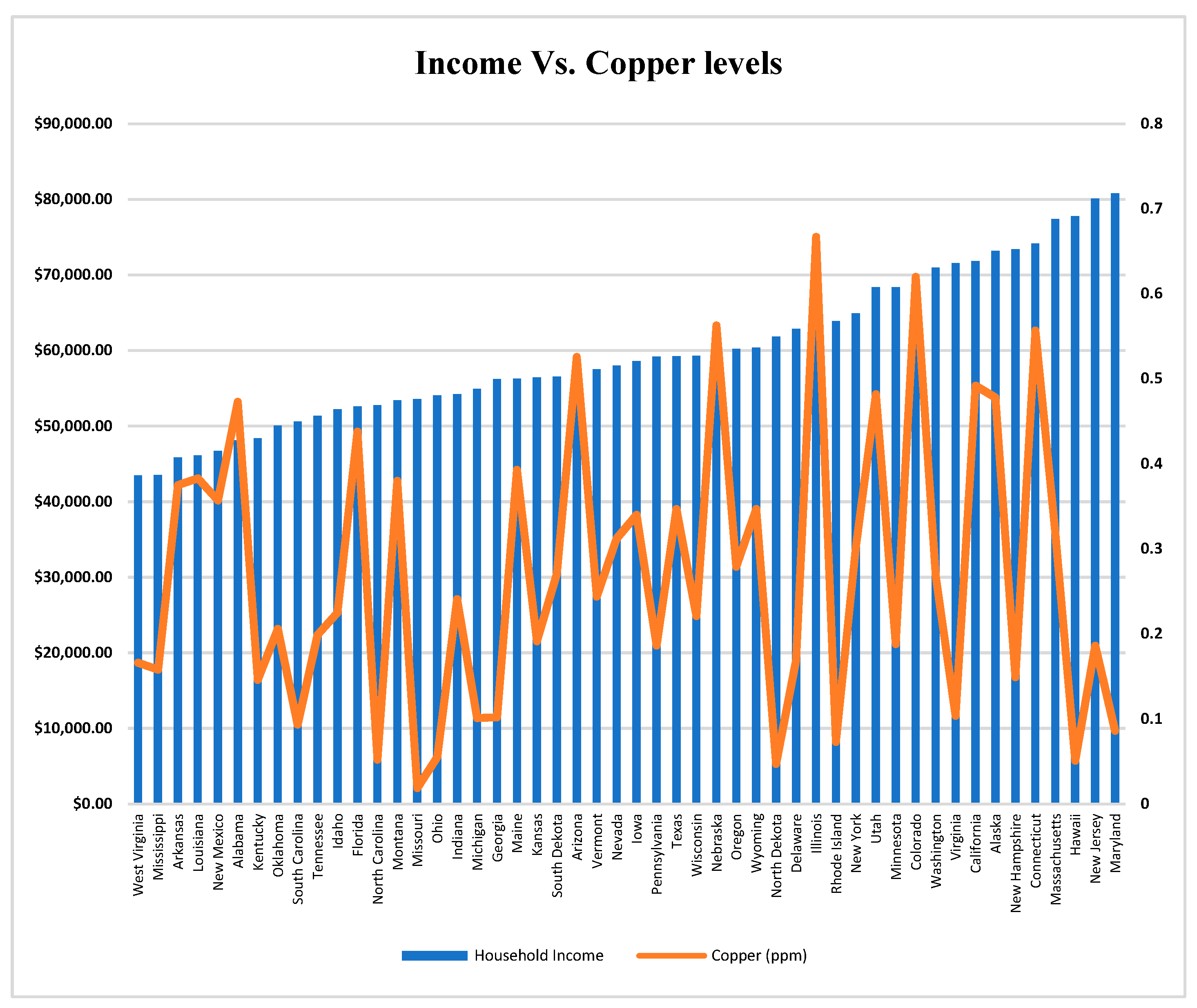
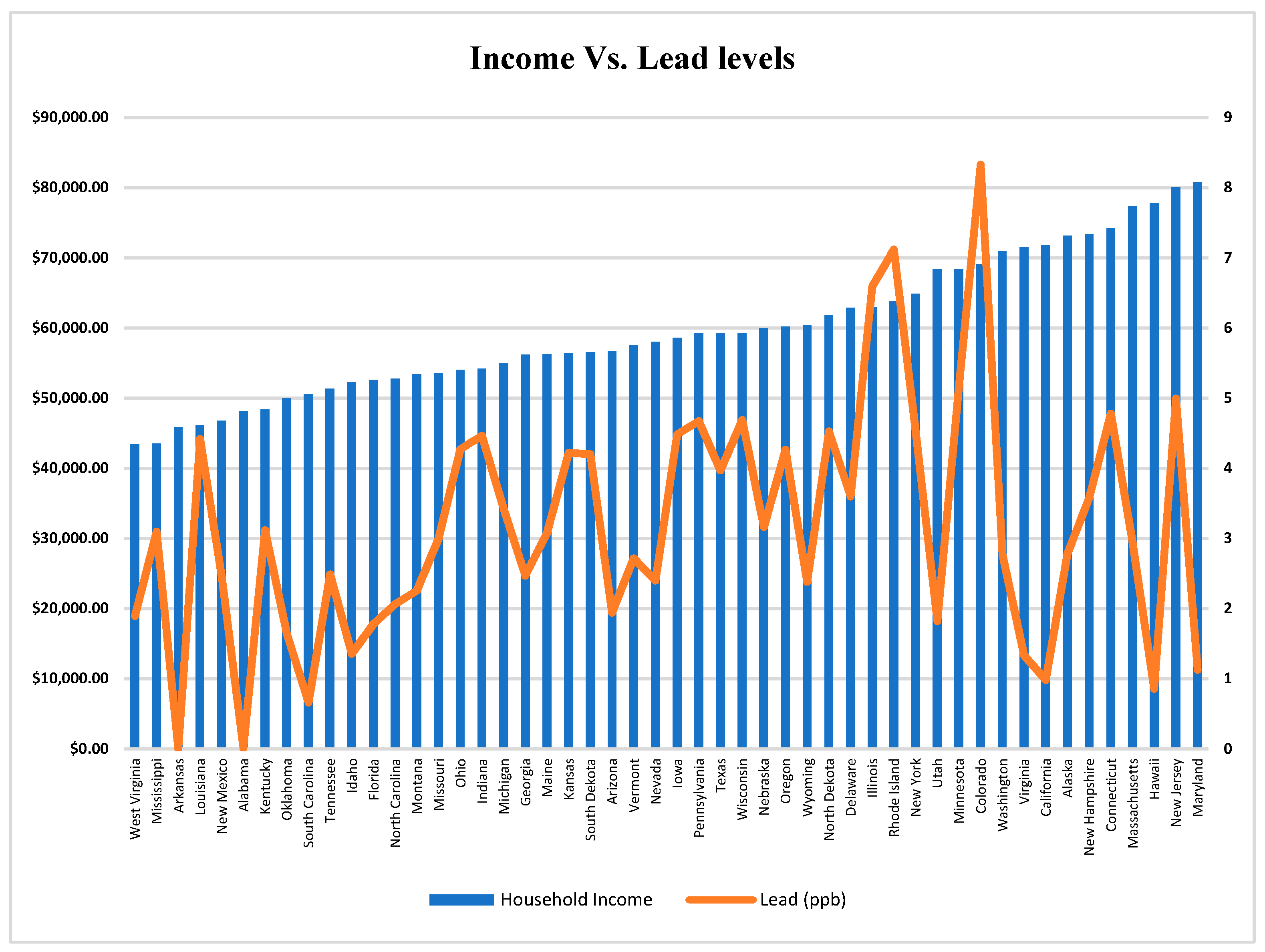
Although a direct correlation was not observed, higher income states demonstrated lower copper levels when compared to the states with lower-average household income. Illinois had slightly higher copper levels compared to the other states (Figure 1). When looking at lead levels, a direct correlation and statistically significant variation was found among lower, middle, and higher household income states (Figure 2).
The states with midrange average household incomes ($62,000–$68,000) had significantly higher lead levels in their drinking water compared to states with higher- and lower-average household incomes. Colorado, Illinois, and Rhode Island had lead levels that were relatively higher than lead levels in the other states. Hence, it was determined that elevated lead levels were much more prevalent among middle income communities.
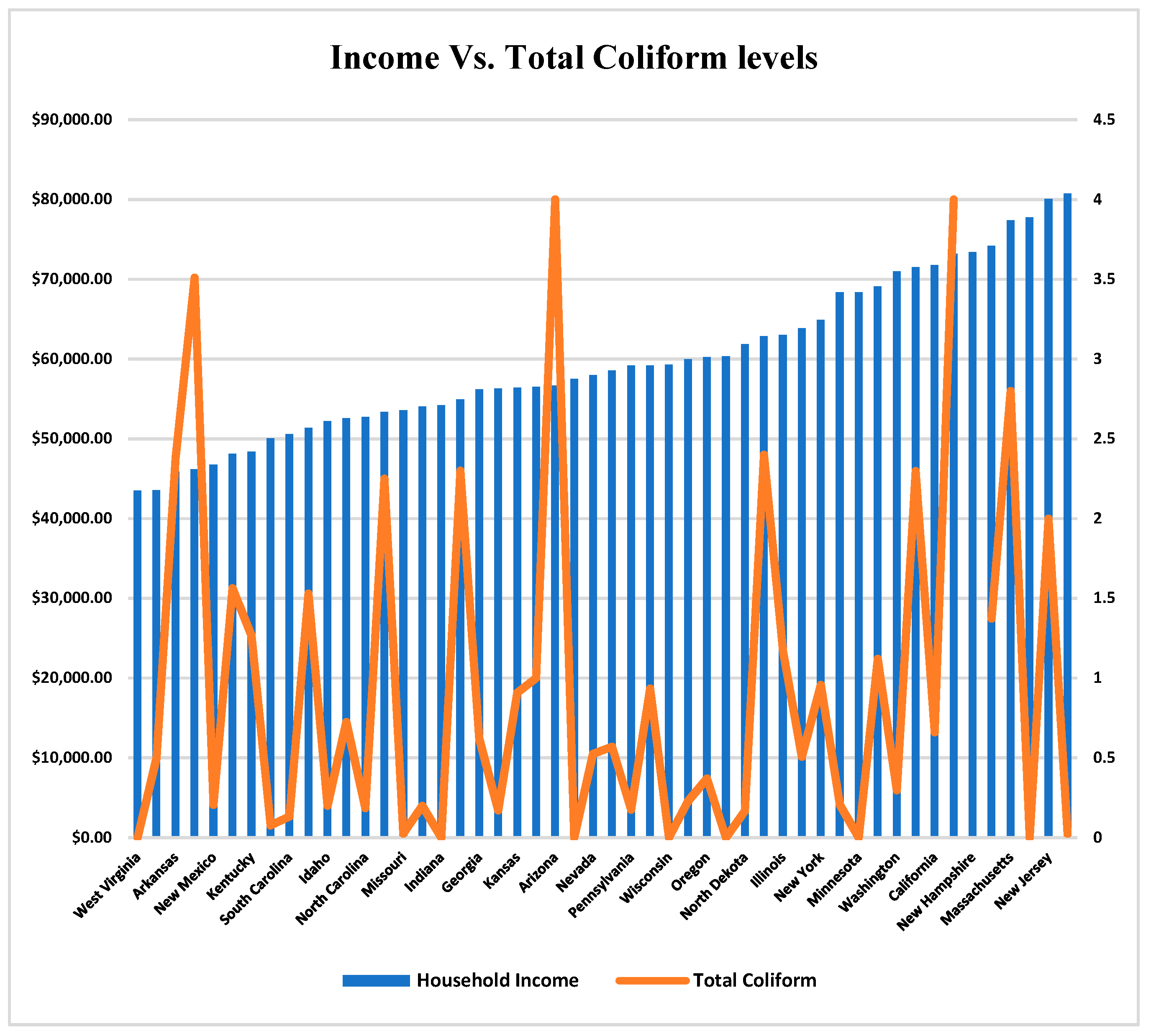
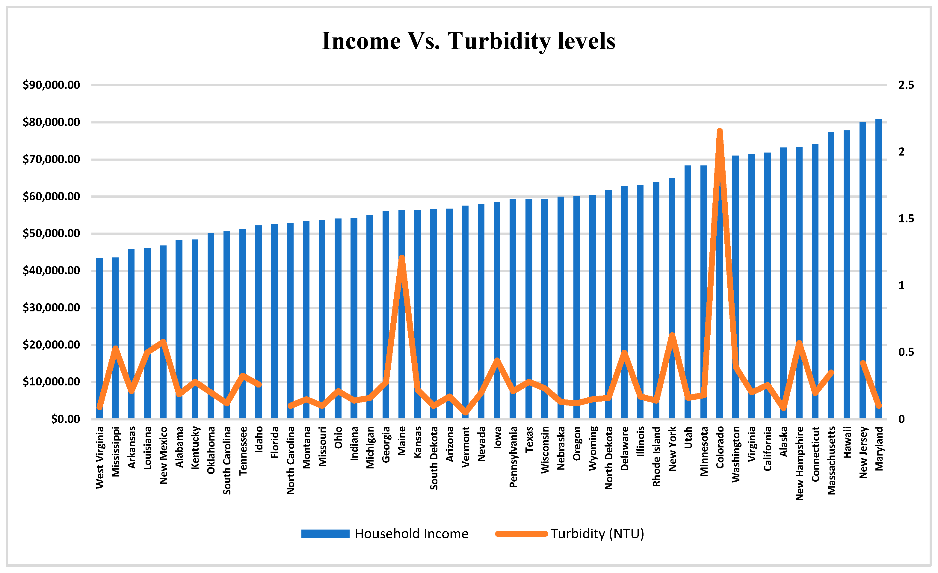
Total coliform levels, on the other hand, were the lowest among middle income groups across the states when compared to higher income groups (Figure 3), although several higher income states demonstrated lower positive total coliform. Elevated positive coliform levels were seen among lower, middle, and upper income brackets in Louisiana, Arizona, and Alaska, respectively. Turbidity levels (Figure 4) were observed to be the lowest among middle income household communities in various states. Colorado and Maine’s turbidity levels were higher than those of the other states. No reports on turbidity levels were available for Florida and Hawaii.
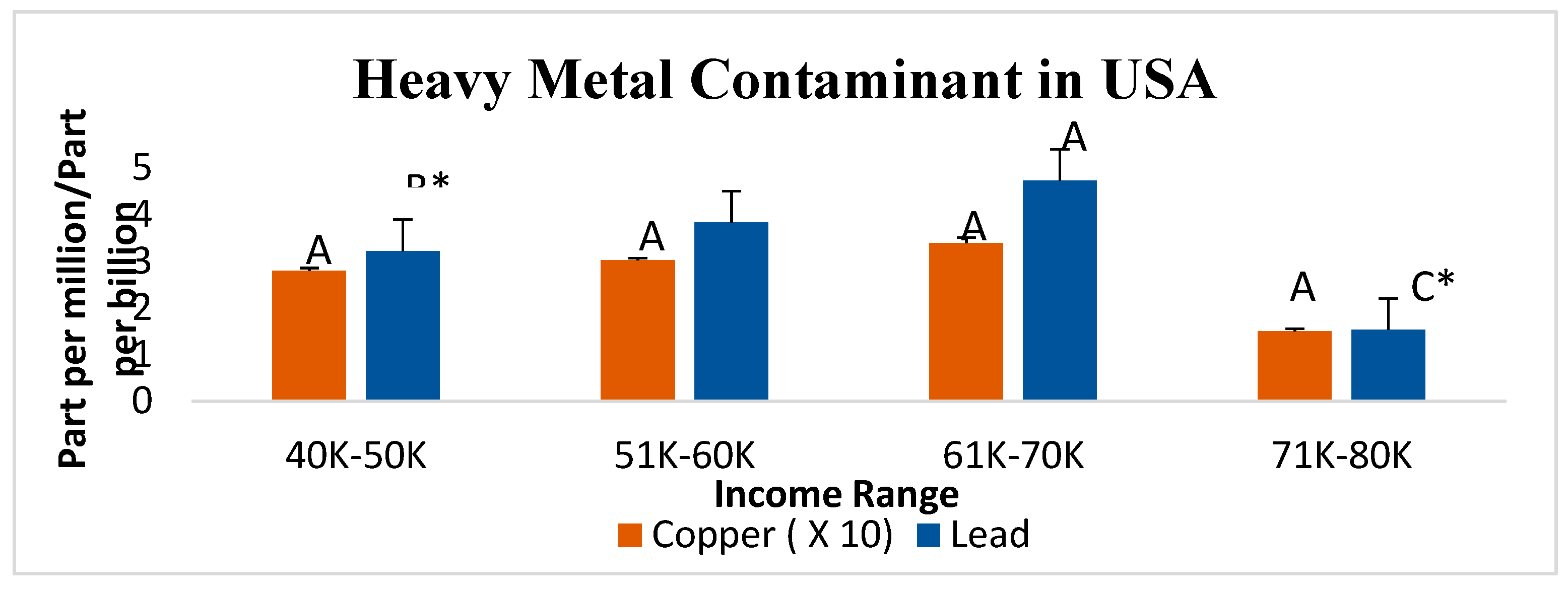
The statistical analyses of contaminant data (p < 0.05, Tukey-adjusted ANOVA) are represented in Figure 5, Figure 6 and Figure 7. The Tukey grouping (a single-step statistical comparison test used to determine significantly different means values) was utilized to indicate the difference among lead and copper means for each income group. The group with the highest level of lead was given the letter A. All other income groups were further compared to group A and to other groups. Groups that share the same letters did not vary significantly in lead or copper levels. Groups denoted with letters B and C indicate significant variation in lead levels. Furthermore, comparisons significant at the 0.05% (95% confidence limits) are represented by an asterisk (*). Statistical significance in lead levels was observed between income ranges of $71,000–$80,000; $51,000–$60,000; and $40,000–$50,000 (Figure 5). The data related to lead in the various states were statistically significant, per Tukey’s test (95% confidence limits), while the data related to copper were not significant statistically.
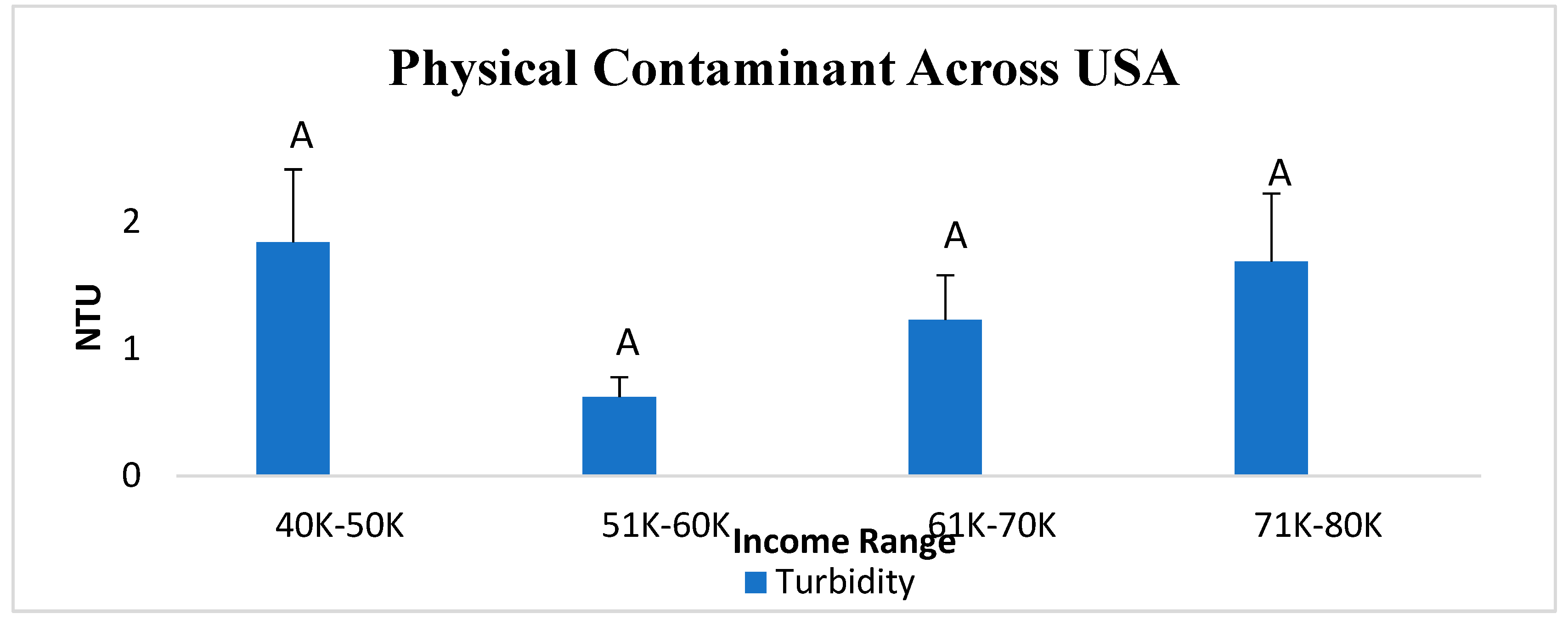
Similarly, the Tukey grouping was utilized to indicate statistical significance level among each income group for the presence of total coliform (Figure 6) and the turbidity level (Figure 7). Means denoted by the same letter (A) were not significantly different.
The communities with the highest average household incomes had significantly lower lead levels in their drinking water when compared to lower income groups. This is consistent with the data plotted in Figure 2. Although copper levels seemed to show the same patterns as lead on the histogram, Tukey’s grouping indicated that the difference in copper means for each income group was not statistically significant. This demonstrates that the individual data points for the copper levels in different income groups shared similarities; hence, the lack of significant variation. No statistical significance was observed in the total coliform or turbidity levels as they correlated to average household income (Figure 6 and Figure 7).
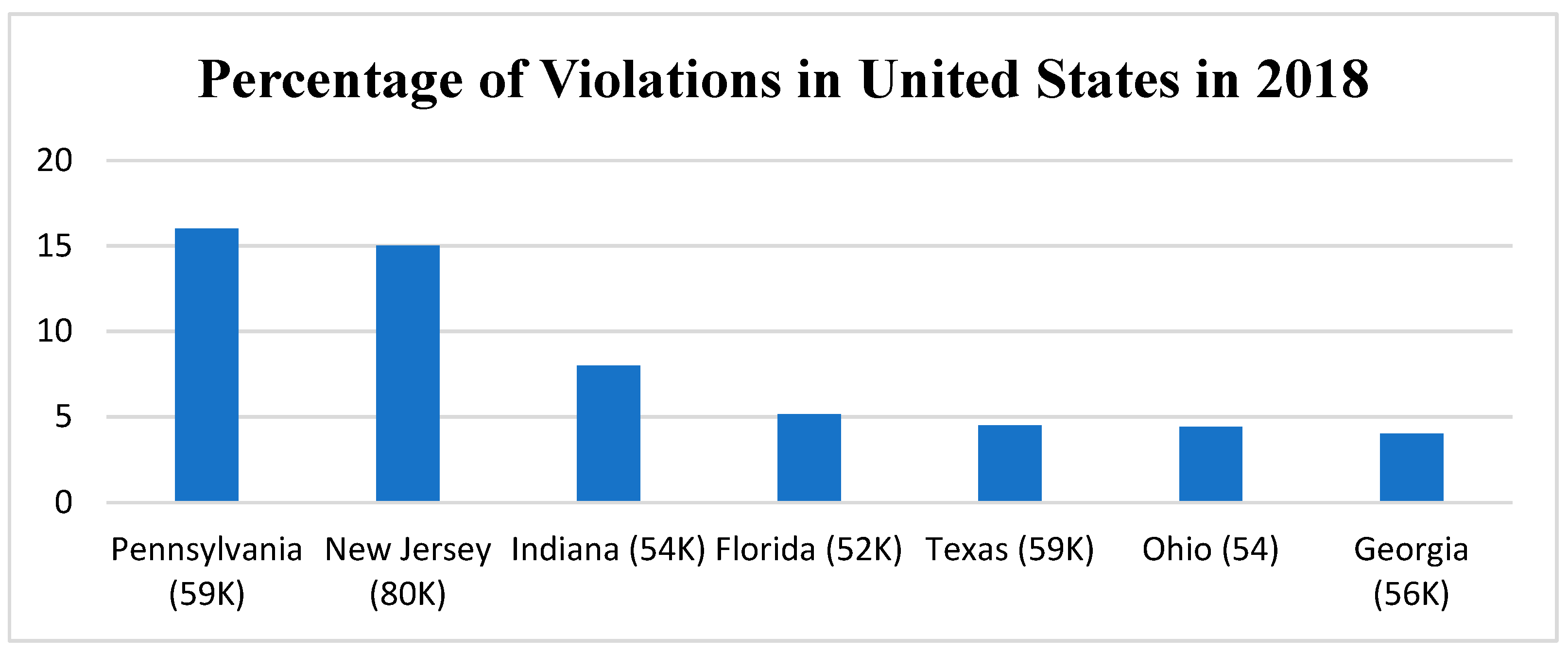
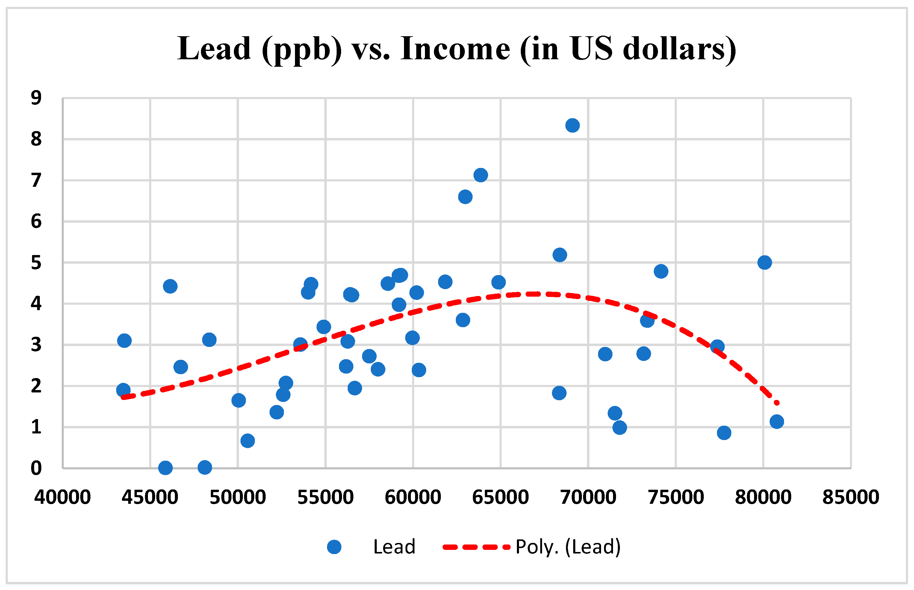
Figure 8 shows the states with the most violations, considering all contaminants. The middle income groups were observed to have the most violations, while the higher income groups had violations in only one state (New Jersey). The number of violations in New Jersey were, however, considered a statistical outlier, as this pattern was not seen any other state within the higher income group. This discrepancy was likely contributed by the water source. The highest violations were observed in the State of Pennsylvania. To further examine the spread of lead levels in each state, a scatter plot was utilized, and the majority of high lead levels in drinking water were clustered among the middle income states. The pattern of data dispersion resembled a bell-shaped curved, with low and high income states having the lowest lead levels (Figure 9).
4. Conclusions
Clean water is a basic necessity and is important for the health and wellbeing of the general populace. A lack of clean drinking water is a significant public health concern. There are many factors that play a role in the quality of water being offered to consumers, such as water source, composition, and water system infrastructure. Feasibility and availability of clean drinking water is a matter of social justice and every citizen should be given an equal right.
Previous research had suggested that individuals living in rural areas may be consuming unregulated and contaminated water. In this study, quantitative measures were taken to explore the role of socioeconomic background on drinking water quality. Statistical significance was observed in elevated lead levels, in that higher income groups outperformed lower-average household income groups. The middle income group was more susceptible to having higher lead levels compared to the other income groups. In addition, middle income groups had repeated water quality violations. New Jersey (in the higher income group) had a significant number of violations. This study showed that some variation in drinking water quality existed among different income groups. Practical applications/interventions of this study include helping environmentalists and water agencies to determine avenues to provide appropriate control services where lead levels are high. In addition, framework studies can be conducted to determine ways in which the disadvantaged communities can be serviced more efficiently, to ensure that water quality disparities are reduced as much as possible.
It is important for this water quality information to be shared with the public to ensure an appropriate level of trust toward the resource, as well as to avoid disparities among households with different income levels [22]. The Environmental Protection Agency (EPA) is the primary authority in the United States that sets standards for drinking water quality and oversees states, localities, and water suppliers in implementing those standards. Information obtained from the present study could be used to draft guidelines in order to keep the population better informed of drinking water quality in their areas, and to ensure that all consumers are aware of chemical and biological contaminants, as well as the risks associated with drinking water. Our study could be used to support ordinances issued by the EPA, such as providing updated information on the various aspects of drinking water to the population through the districts’ water supply websites. Furthermore, this investigation can serve as a guide for lawmakers to allocate resources toward the improvement of infrastructure in communities with poor water quality.
Author Contributions
Conceptualization, R.B.; data curation, K.K., S.G., and R.B.; formal analysis, K.K., S.G., and R.B.; funding acquisition, R.B. and S.G.; investigation, K.K., S.G., and R.B.; methodology, K.K., S.G., and R.B.; project administration, R.B.; software, K.K.; supervision, R.B. and S.G.; writing—original draft, K.K.; writing—review and editing, K.K., S.G., and R.B. All authors have read and agreed to the published version of the manuscript.
Funding
This research was funded by the USDA National Institute of Food and Agriculture, Grant# TENX-1608-FS. We thank US Department of Education, Title III Part B, grant number P031B090214 for partial financial support.
Conflicts of Interest
The authors declare no conflicts of interest regarding the publication of this paper.
References
- Watson, K.; Garrett, M. Clean Drinking Water a Bigger Global Threat than Climate Change, EPA’s Wheeler says. 2019. Available online: https://www.cbsnews.com/news/epa-administrator-andrew-wheeler-exclusive-interview/ (accessed on 2 January 2020).
- Dieter, C.A.; Maupin, M.A. Public Supply and Domestic Water Use in the United States, 2015. 2017. Available online: https://doi.org/10.3133/ofr20171131 (accessed on 2 January 2020).
- SDWA. Background on Drinking Water Standards in the Safe Drinking Water Act; Environmental Protection Agency (EPA): Washington, DC, USA, 2017. Available online: https://www.epa.gov/dwstandardsregulations/background-drinking-water-standards-safe-drinking-water-act-sdwa (accessed on 2 January 2020).
- Dubrovsky, N.M.; Kratzer, C.R.; Brown, L.R.; Gronberg, J.M.; Burow, K.R. Water Quality in the San Joaquin-Tulare Basins, California, 1992–95. U.S. Geological Survey Circular 1159. 1998. Available online: http://pubs.usgs.gov/circ/circ1159/ (accessed on 9 February 2020).
- Beni, R.; Guha, S.; Hawrami, S. Drinking Water Disparities in Tennessee: The Origins and Effects of Toxic Heavy Metals. J. Geosci. Environ. Prot. 2019, 7, 135–146. [Google Scholar] [CrossRef] [Green Version]
- Environmental Protection Agency (EPA). Ground Water and Drinking Water: National Primary Drinking Water Regulations. 2020. Available online: https://www.epa.gov/ground-water-and-drinking-water/national-primary-drinking-water-regulations (accessed on 23 February 2020).
- Yousef, S.; Eapen, V.; Zoubeidi, T.; Kosanovic, M.; Mabrouk, A.A.; Adem, A. Learning Disorder and Blood Concentration of Heavy Metals in the United Arab Emirates. Asian J. Psychiatry 2013, 6, 394–400. [Google Scholar] [CrossRef] [PubMed]
- Nigg, J.; Knottnerus, M.; Martel, M.M.; Nikolas, M.; Cavanagh, K.; Karmaus, W.; Rappley, M.D. Low Blood Lead Levels Associated with Clinically Diagnosed Attention-Deficit/Hyperactivity Disorder and Mediated by Weak Cognitive Control. Biol. Psychiatry 2008, 63, 325–331. [Google Scholar] [CrossRef] [PubMed] [Green Version]
- Feldman, R.G.; White, R.F. Lead Neurotoxicity and Disorders of Learning. J. Child Neurol. 1992, 7, 354–359. [Google Scholar] [CrossRef] [PubMed]
- Szewzyk, U.; Szewzyk, R.; Manz, W.; Schleifer, K.-H. Microbiological Safety of Drinking Water. Annu. Rev. Microbiol. 2000, 54, 81–127. [Google Scholar] [CrossRef] [PubMed]
- Environmental Protection Agency (EPA). 2018 Edition of the Drinking Water Standards and Health Advisories Tables. 2018. Available online: https://www.epa.gov/sites/production/files/2018-03/documents/dwtable2018.pdf (accessed on 2 January 2020).
- Moe, C.L.; Sobsey, M.D.; Samsa, G.P.; Mesolo, V. Bacterial Indicators of Risk of Diarrhoeal Disease from Drinking-Water in the Philippines. Bull. World Health Organ. 1991, 69, 305–317. [Google Scholar] [PubMed]
- Fattal, B.; Gutman-Bass, N.; Agursky, T.; Shuval, H.I. Evaluation of Health Risk Associated with Drinking Water Quality in Agricultural Communities. Water Sci. Technol. 1988, 20, 409–415. [Google Scholar] [CrossRef]
- Strauss, B.; King, W.; Ley, A. A Prospective Study of Rural Drinking Water Quality and Acute Gastrointestinal Illness. BMC Public Health 2001, 1, 8. [Google Scholar] [CrossRef] [PubMed] [Green Version]
- World Health Organization (WHO). Water Quality and Health- Review of Turbidity: Information for Regulators and Waste Water Suppliers. 2017. Available online: https://apps.who.int/iris/bitstream/handle/10665/254631/WHO-FWC-WSH-17.01-eng.pdf?sequence=1&isAllowed=y (accessed on 27 February 2020).
- Environmental Protection Agency (EPA). Ground Water and Drinking Water: National Primary Drinking Water Regulations. 2018. Available online: https://www.epa.gov/ground-water-and-drinking-water/national-primary-drinking-water-regulations#Microorganisms (accessed on 2 January 2020).
- Olmstead, S.M. Thirsty Colonias: Rate Regulation and the Provision of Water Service. Land Econ. 2004, 80, 136–150. [Google Scholar] [CrossRef]
- Balazs, C.; Morello-Frosch, R.; Hubbard, A.; Ray, I. Social Disparities in Nitrate-Contaminated Drinking Water in California’s San Joaquin Valley. Environ. Health Perspect. 2011, 119, 1272–1278. [Google Scholar] [CrossRef] [Green Version]
- Balazs, C.L.; Morello-Frosch, R.; Hubbard, A.E.; Ray, I. Environmental Justice Implications of Arsenic Contamination in California’s San Joaquin Valley: A Cross-Sectional, Cluster-Design Examining Exposure and Compliance in Community Drinking Water Systems. Environ. Health 2012, 11, 84. [Google Scholar] [CrossRef] [Green Version]
- The United States Census Bureau. S1901: Income in the Past 12 Months. Households-Total-Estimate. 2018. Available online: https://data.census.gov/cedsci/map?q=S1901%3A%20INCOME%20IN%20THE%20PAST%2012%20MONTHS%20%28IN%202018%20INFLATION-ADJUSTED%20DOLLARS%29&table=S1901&tid=ACSST1Y2018.S1901&hidePreview=false&cid=S1901_C01_001E&vintage=2018&lastDisplayedRow=93&layer=state&g=0400000US10,12,13,15,16,17,18,19,20,21,22,23,24,25,26,27,28,29,30,31,32,33,34,35,36,37,38,39,40,41,42,44,45,46,47,48,49,50,51,53,54,55,56,72,05,02,08,01,06,09,04&t=Income%20%28Households,%20Families,%20Individuals%29&y=2018 (accessed on 18 November 2019).
- Lowry, R. One way Analysis of Variance for Independent Samples. 2007. Available online: https://web.archive.org/web/20081017161620/http://faculty.vassar.edu/lowry/ch14pt2.html (accessed on 4 January 2020).
- Dettori, M.; Azara, A.; Loria, E.; Piana, A.; Masia, M.D.; Palmieri, A.; Cossu, A.; Castiglia, P. Population Distrust of Drinking Water Safety. Community Outrage Analysis, Prediction and Management. Int. J. Environ. Res. Public Health 2019, 16, 1004. [Google Scholar] [CrossRef] [PubMed] [Green Version]
Figure 1.
Correlation between average household income and copper levels (ppm). Several high income states have lower copper levels in their drinking water when compared to low income states where copper levels are much higher.
Figure 1.
Correlation between average household income and copper levels (ppm). Several high income states have lower copper levels in their drinking water when compared to low income states where copper levels are much higher.

Figure 2.
Correlation between average household income and lead levels (ppb). High income states have significantly lower lead levels in their drinking water compared to low income and middle income communities.
Figure 2.
Correlation between average household income and lead levels (ppb). High income states have significantly lower lead levels in their drinking water compared to low income and middle income communities.

Figure 3.
Correlation between average household income and total coliform (% positive samples). Higher total coliform levels were seen in middle income and low income states, while the higher income states demonstrated lower levels of total coliform in their drinking water.
Figure 3.
Correlation between average household income and total coliform (% positive samples). Higher total coliform levels were seen in middle income and low income states, while the higher income states demonstrated lower levels of total coliform in their drinking water.

Figure 4.
Correlation between average household income and turbidity levels (NTU). Turbidity level was low in all states, regardless of income, with the exception of Colorado, which demonstrated a significantly higher turbidity level.
Figure 4.
Correlation between average household income and turbidity levels (NTU). Turbidity level was low in all states, regardless of income, with the exception of Colorado, which demonstrated a significantly higher turbidity level.

Figure 5.
ANOVA test results for average household income versus copper and lead across the United States. Statistical analyses of contaminant data (p < 0.05, Tukey-adjusted ANOVA) indicated significant differences in lead levels in drinking water among states, corresponding to different income brackets. The statistical variation among the income brackets are indicated by A, B, and C, and the statistical significance is denoted by an asterisk (*).

Figure 6.
ANOVA test results for average household income as related to coliform across the United States. Numerical analyses of contaminant data (p < 0.05, Tukey-adjusted ANOVA) did not indicate statistically significant variation.
Figure 6.
ANOVA test results for average household income as related to coliform across the United States. Numerical analyses of contaminant data (p < 0.05, Tukey-adjusted ANOVA) did not indicate statistically significant variation.

Figure 7.
ANOVA test results for average household income as related to turbidity across the United States. Numerical analyses of contaminant data (p < 0.05, Tukey-adjusted ANOVA) did not indicate statistically significant variation.
Figure 7.
ANOVA test results for average household income as related to turbidity across the United States. Numerical analyses of contaminant data (p < 0.05, Tukey-adjusted ANOVA) did not indicate statistically significant variation.

Figure 8.
Percent violations in different states, with average household income in parentheses. States in the middle income bracket had significantly higher violations, while only one high income state (New Jersey) had a significantly high number of violations.
Figure 8.
Percent violations in different states, with average household income in parentheses. States in the middle income bracket had significantly higher violations, while only one high income state (New Jersey) had a significantly high number of violations.

Figure 9.
Scatter plot of lead levels versus income, which resembles a bell-shaped curve. The highest levels of lead are densely present among the middle income communities, while lower levels of lead are present among lower and higher income communities.
Figure 9.
Scatter plot of lead levels versus income, which resembles a bell-shaped curve. The highest levels of lead are densely present among the middle income communities, while lower levels of lead are present among lower and higher income communities.


Table 1.
Primary surface water sources for the metropolitan areas of each state.
| States | Surface Water Sources | States | Surface Water Sources |
|---|---|---|---|
| Alabama | Tallapoosa River | Montana | Yellowstone River |
| Alaska | Last Chance Basin | Nebraska | Platte River |
| Arizona | Salt River, Upper Lake Mary | Nevada | Kings Canyon Creek |
| Arkansas | Lake Maumelle | New Hampshire | Penacook Lake |
| California | Sacramento River, Owens River | New Jersey | Delaware River |
| Colorado | South Platte River, Blue River | New Mexico | Santa Fe Watershed |
| Connecticut | Farmington River, Nepaug River | New York | Alcove Reservoir |
| Delaware | Delaware River | North Carolina | Falls Lake Reservoir |
| Florida | Floridan Aquifer | North Dakota | Missouri River |
| Georgia | Chattahoochee River, Lake Lanier | Ohio | Scioto River |
| Hawaii | Koolau Watershed | Oklahoma | Lake Overholser |
| Idaho | Boise River | Oregon | North Santiam River |
| Illinois | Lake Springfield | Pennsylvania | DeHart Reservoir |
| Indiana | White River, Geist Reservoir | Rhode Island | Scituate Reservoir |
| Iowa | Raccoon River, Des Moines River | South Carolina | Lake Murray |
| Kansas | Kansas River | South Dakota | High Plains Aquifer |
| Kentucky | Kentucky River | Tennessee | Cumberland River |
| Louisiana | Southern Hills Aquifer | Texas | Colorado River, Trinity River |
| Maine | Kennebac River | Utah | Wasatch Front Streams |
| Maryland | Magothy Formation Aquifer | Vermont | Lake Champlain |
| Massachusetts | Quabin Reservoir | Virginia | James River |
| Michigan | Saginaw Aquifer | Washington | McAllister Wellfield |
| Minnesota | Mississippi River | West Virginia | Elk River |
| Mississippi | Ross-Barnett Reservoir | Wisconsin | Sandstone Aquifer |
| Missouri | Missouri River | Wyoming | Laramie Mountain Stream |
© 2020 by the authors. Licensee MDPI, Basel, Switzerland. This article is an open access article distributed under the terms and conditions of the Creative Commons Attribution (CC BY) license (http://creativecommons.org/licenses/by/4.0/).
Share and Cite
MDPI and ACS Style
Karim, K.; Guha, S.; Beni, R. Comparative Analysis of Water Quality Disparities in the United States in Relation to Heavy Metals and Biological Contaminants. Water 2020, 12, 967. https://doi.org/10.3390/w12040967
AMA Style
Karim K, Guha S, Beni R. Comparative Analysis of Water Quality Disparities in the United States in Relation to Heavy Metals and Biological Contaminants. Water. 2020; 12(4):967. https://doi.org/10.3390/w12040967
Chicago/Turabian StyleKarim, Kaleh, Sujata Guha, and Ryan Beni. 2020. "Comparative Analysis of Water Quality Disparities in the United States in Relation to Heavy Metals and Biological Contaminants" Water 12, no. 4: 967. https://doi.org/10.3390/w12040967
Note that from the first issue of 2016, this journal uses article numbers instead of page numbers. See further details here.