Exploring Empirical Linkage of Water Level–Climate–Vegetation across the Three Georges Dam Areas


School of Hydropower and Information Engineering, Huazhong University of Science and Technology, Wuhan 430074, China
*
Authors to whom correspondence should be addressed.
Water 2020, 12(4), 965; https://doi.org/10.3390/w12040965
Submission received: 7 February 2020
/
Revised: 6 March 2020
/
Accepted: 26 March 2020
/
Published: 28 March 2020
(This article belongs to the Section Hydrology)
Abstract
:The Three Georges Dam (TGD) has brought many benefits to the society by periodically changing the water level of its reservoir (TGR). Water discharging regularly takes places in the falling season when the downstream of the Yangtze River is drying. The TGD, the world’s largest hydroelectric project, can greatly mitigate the risk of flood caused by extreme precipitation with the prior discharging policy applied in the preflood season. At the end of flood season, water impounding in the storage season can help resist a drought the next year. However, owing to the difficulty in mining causality, the considerable debate about its environmental and climatic impacts have emerged in much of the empirical and modeling studies. We used causal generative neural networks (CGNN) to construct the linkage of water level–climate–vegetation across the TGD areas with a ten-year daily remotely sensed normalized difference vegetation index (NDVI), gauge-based precipitation, temperature observations, water level and streamflow. By quantifying the causality linkages with a non-linear Granger-causality framework, we find that the 30-days accumulated change of water level of the TGR significantly affects the vegetation growth with a median factor of 31.5% in the 100 km buffer region. The result showed that the vegetation dynamics linked to the water level regulation policy were at the regional scale rather than the local scale. Further, the water level regulation in the flood stage can greatly improve the vegetation growth in the buffer regions of the TGR area. Specifically, the explainable Granger causalities of the 25 km, 50 km, 75 km and 100 km buffer regions were 21.72%, 19.24%, 17.31% and 16.03%, respectively. In the falling and impounding stages, the functionality of the TGR that boosts the vegetation growth were not obvious (ranging from 6.1% to 8.3%). Overall, the results demonstrated that the regional vegetation dynamics were driven not only by the factor of climate variations but also by the TGR operation.
1. Introduction
The ongoing development of hydropower dams in the Yangtze River has been bringing debates about what priority the sustainability of economic development and environment protection should be taken for a policy maker. Specifically, the Three George Dam (TGD), the world largest hydropower project, provides as many benefits to the Yangtze River economic belt as flood control, clean water and green energy supply, navigation and sediment management in China. The Three George plant has the total installed capacity of 22.5 GW and an annual power generation of approximately 100 Tw [1]. Regardless of the contribution made for the national economic development, the ecological and environmental influence have attracted significant attention from researchers [2,3,4]. A scientific report indicated that the dramatic recession in China’s largest freshwater lake, Poyang Lake, has a strong linkage with TGD regulation. TGD regulation explains 56.3% of the lake level decrease over the past decade [2]. However, a recent study concluded that the recent decade’s lake decline in the Yangtze Plain is a major result of climate variability, instead of direct human interventions. TGD causes no substantial climate variations downstream due to limited alternations of the lake surface area [4]. Importantly, the policy maker needs objective and consistent causality linkages to boost the economy while keeping the environment sustainable.
Inferring such causality among anthropogenic activities, climate indicators and environmental responses is difficult. Classical statistical methods try to separate the impact factors from the target variables. For example, to quantify the impact between climate variables and human factors on vegetation dynamics, Qu divided the NDVI time series into the reference period and conservation period [5]. Then, Qu used a linear regression model to represent the maximum association between the climate variables and NDVI in the reference period. Finally, the obtained regression coefficients were used to check whether the trend of the residuals between the observed NDVI and predicted NDVIs exists or not in the second period. The assumption is that if there were no trend, the observed changes in vegetation were only affected by climatic factors, while the decreasing and ascending trends indicate the negative and positive human impact, respectively. Zhao used a double mass curve analysis to assess nature and anthropogenic influences on water discharge and sediment load in the Yangtze River [6]. Reservoir regulation played a significant role in modifying peak flows in the wet season and low flows in the dry season, and the irrigation activities in the cropped or vegetated area would affect the overall hydrology condition [7,8]. However, these statistical methods are often too simplistic to represent complex climate–vegetation causality due to linearity assumptions. Based on Reichenbach’s common cause principle [9], casual inference methods aim to discover and quantify the causal interdependencies of complex systems [10]. Questions such as “How much does TGD contribute to the Yangtze lake decline?” and “Is climate a dominant factor to the Yangtze lake decline?” can be objectively answered [11]. Granger causality (GC) is the type of tool that has been widely adopted in several science discoveries, such as in feedback mechanisms between soil moisture and precipitation [11], or in relationships between the atmosphere and terrestrial biosphere [12]. The extensions of GC includes non-linear causality mining [13], which can explore the causality between time series in terms of predictability: If time series X cause time series Y, the inclusion of the past of both X and Y should boost the prediction of the presence of Y compared to exclusively using the past of Y. The non-linear GC framework overcomes the lagged correlations that arise from the autocorrelation, seasonality and inter-annual variability, and are applicable to large datasets with excellent computational scalability. There also emerged deep learning-based casual inference methods in recent years [10].
In this study, we aim to investigate empirical evidence of contrasting water level–climate–vegetation feedback across the TGD area by using causal inference methods. The Three Gorges Reservoir (TGR) covers the reach of the Yangtze River between Chongqing and Yichang with a total water surface area of 1080 km2 at the water level of 175 m [14]. After two tentative impounding operations to the elevations of 135 m and 156 m above the sea level at 10 June 2003, and 27 October 2006, respectively, the TGR started impounding water after the flood season with the water level of 175 m above mean sea level reached 26 October 2010. The water level would change regularly for water supply during the dry season, shipping navigation between late March to middle April, discharging water to 145 m for flood preparation, flood peak smoothing during floods and impounding water during the storage season. Although, few works have reported the influence of climate variability and TGR operations on streamflow in the Yangtze River [15], and the linkage of water level with climate and vegetation feedback is also poorly understood. To this end, we answer the questions as follows: (1) Does the vegetation of the TGR area (TGRA) undergo furious change after the regular TGR operation? (2) To what extent do anthropogenic activities such as water level regulation causes the vegetation change? (3) How many days of the accumulated water level cause the vegetation changes? (4) Does the causality still hold in the drying stage, impounding stage and falling stage of the TGRA?
The study consists of four parts corresponding with the four questions. In the first part, we use satellite observations to capture continuous and daily NDVI from Moderate Resolution Imaging Spector radiometer (MODIS). The spatiotemporal variation of vegetation coverage of the TGRA under the coupling effect of the climate and anthropogenic factors is explored. In the second part, we use generative neural networks to build causality linkages among daily streamflow, averaged air temperature, precipitation, NDVI, and accumulated water level. Then, the encoded linkages are further investigated with the non-linear Granger-causality framework in the third part. In the last part, we investigate whether the causality still hold in these stages. The organization of this study is as follow. The study area is introduced in Section 2. The data and methods are presented in Section 3. The results and analysis are described in Section 4. Finally, the discussion and conclusions are given in Section 5.
2. Study Area
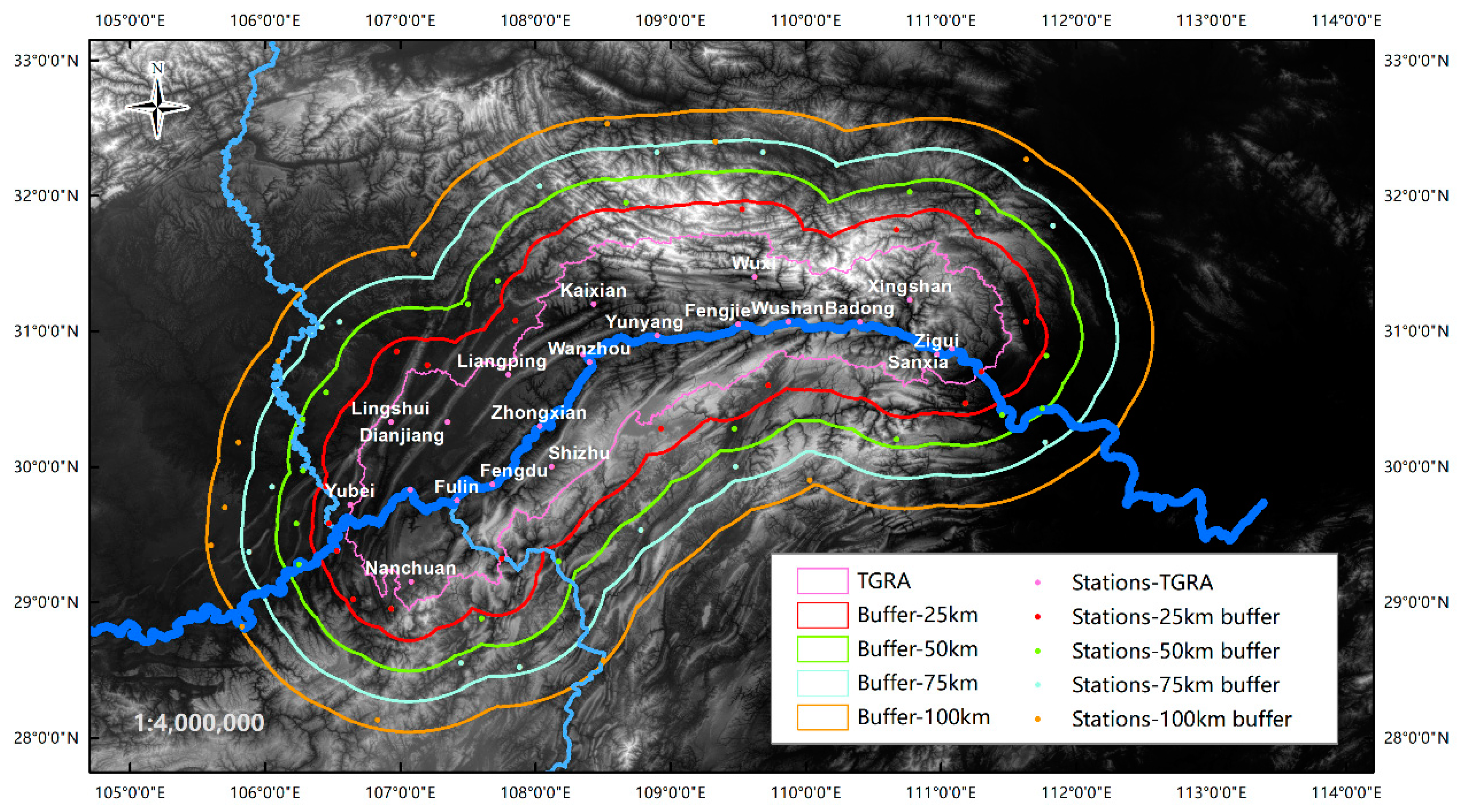
Based on Wu’s research [16], the climatic effect of the TGR is on the regional scale (~100 km); we investigate the regional feedback between the atmosphere and terrestrial biosphere under the full operation of the TGR. In this study, we focus on the buffered area of the TGR area at 28° N–33° N and 105° E–113° E (Figure 1). From the innermost to the outermost, the buffered area consists of five regions. The innermost region is the TGRA with a very complex geomorphology. The TGRA includes the regions of Yichang, Zigui, Xingshan, Badong, Wushan, Wuxi, Fengjie, Yunyang, Wanzhou, Kaixian, Zhongxian, Shizhu, Fengdu, Changshou, Fuling, Wulong, Yubei, Banan, Chongqing and Jiangjin. The terrain skeleton of the mountains of the TGRA was completed after the Yanshan orogeny in the Late Jurassic. Following the Himalayan orogeny in the Neogene and long-term erosional processes, the area has numerous moderate-to-low-altitude mountains and river valleys [17]. The section from Fengjie to the west of Zigui is topographically the highest, creating the famous Three Gorges (Qutang Gorge, Wu Gorge and Xiling Gorge). The elevation declines westwards and eastwards from the highest part, forming a hilly landscape and moderate altitude mountains, respectively [18]. The elevation of the meteorological stations ranges from 171 m at Badong station to 604 m at Fengjie station. We abbreviate the five regions as TGRA, buffer-25 km, buffer-50 km, buffer-75 km and buffer-100 km. The TGRA contains 21 meteorological stations. The other four regions have 61 stations in total. According to the environment and ecological monitoring bulletins (ECMB) of the Three Gorges office, the full operation of the TGR started from 2008. The average annual precipitation of the TGRA ranges between 723 and 1134 mm, and the average annual temperature ranges between 8.6 and 16.8 °C.
The water level of the TGR changes based on a strict operation rule. We divide the regulated TGR operation into three stages according to Qin’s research [19]. More specifically, in the falling stage starting from January to early June, the water level would decline to no lower than 155 m at the end of April, no higher than 155 m after May 25 and to the base level of 145 m before the flood season. During the flood stage from 10 June to 10 September, the reservoir level would be maintained at a flood limiting level of 145 m, and when the inflow is less than 35,000 m3/s, water is completely released. Otherwise, flood control operations are conducted considering the downstream safety and release capacity of hydro turbines. The storage stage begins at the end of the flood season, with the water level gradually rising to no more than 162 m at the end of September, and to 175 m no earlier than the end of October. From November to December, the reservoir water level would be kept as high as possible if the storage level has already reached the final stage of 175 m, otherwise the water level should continue to rise up to 175 m.
3. Data and Method
Our objective is to quantify the impact of water level on the vegetation phenology of the study area under the full operation of the TGR. Three groups of data are used in the study:
- Satellite-based NDVI for investigating vegetation changes.
- Ground-measured air temperature and precipitation for understanding climate variations.
- Hydrological elements including daily water level and streamflow for mining the causality linkages.
3.1. Vegetation Dynamics Considering Climate Impacts
MOD09GA (v006, USGS, USA) products provide daily gridded surface spectral reflectance of Terra/MODIS band 1–7 corrected for atmospheric conditions. The daily tiles of the MOD09GA product covering the entire China from 2006 to 2015 are used to extract the NDVI for each meteorological station. NDVI is an important indicator of vegetation growth and coverage during the whole period of the growing season in arid and semi-arid regions and can be considered an effective indicator in monitoring vegetation change from regional to global scales [20]. We use NDVI for understanding the vegetation dynamic across the TGD area in this study. The 82 meteorological stations each collected the daily air temperature and precipitations from 1998 to 2018. To investigate the vegetation dynamics associated with the TGR, it was important to separate the effect of the TGR from the large-scale climate impacts. We adopt the method as used in Song’s research [14]. In our study, the regional background was defined as the 100 km spatial buffer from the TGRA. Because the influence of large-scale climates was similar for both the TGRA and the regional background. We removed the large-scale climate impacts by subtracting the mean NDVI for the regional background in each of TGR operation stage. The new time series NDVI of the 21 meteorological stations were used as the input of the Manner–Kendall analysis [21]. Only the statistically significant trends (P ≤ 0.05) were examined
3.2. Constructing Causality Linkages from Multivariate Time Series Data
To explore the directional/indirectional relationships among time series of streamflow, water level, temperature, precipitation and NDVI, we used a deep-learning-based causality inference method in this study. Causal generative neural networks (CGNNs) were used to learn functional causal models (FCMs) directly from noisy data without any preprocessing [22]. FCMs represents a set of equations each characterizing the direct causal relation from the set of causes to an observed variable. Supposing represents a vector of random variables corresponding to the mentioned time series datasets, an FCM based on the vector is a triple , which consists of a set of equations as follows.
where and one term of Equation (1) represents directional causal relation from the set of causes to the observed variable . FCM is described by a certain causal mechanism up to the effects of noise variable drawn after distribution ε, accounting for all unobserved phenomenon. The observed variable interchangeably denotes a node in the directed acyclic graph g and ε is set to the uniform distribution on [0, 1]. The directional linkage from to maps to the directed edge of the generated causality graph g after a learning procedure had been executed. The theoretical causality inference depends on a series of common assumptions, including a causal sufficiency assumption, causal Markov assumption and causal faithfulness assumption [23]. The functionality of these FCMs is to represent a joint distribution of these random variables with considerations of interventional distributions [24]. Specifically, suppose the joint distribution of the random variable vector is , and further assume that the joint density distribution of ) is integral on a compact subset of . Letting g be the directed acyclic graph such that can be factorized along g.
Based on vector quantile regression [25] and the topological order of g, the proof that there exists a vector of causal mechanism such that the joint distribution equals the generative model defined from the FCMs can be testified. Another important proposition indicates that there exists a generative neural network that can approximate these FCMs [22]. To build the generative neural network from the random variables, we first used a score-based approach coupling with Chickering’s two-phases greedy algorithm [26] to minimize the distance between the joint distribution of ground-truth data and the joint distribution estimated from sample data. Second, we performed the maximum mean discrepancy(MMD) as the kernel method to test whether these distributions are different, which facilitates the backpropagation algorithms to be applied for obtaining the network architecture [27]. Third, we applied the feature-wise kernelized lasso method in the high dimensional feature selection to overcome the curse of dimensionality [28]. The greedy procedure for finding the ground truth graph and functional casual mechanism involves three steps: first we orient each pair of nodes by selecting the associated 2-variable generative neural network with the best score; then we follow the paths from a random set of nodes of a skeleton until reaching all of the nodes; additionally, we modify the orientation to improve the score without making a cycle during the iteration learning procedure. The implementation of CGNN for constructing the causality graph from the time series datasets also includes three procedures: first, the MMD algorithm and generative neural networks were used to build a skeleton of the causality graph [27]. The skeleton is an undirected graph and of which each variable has been applied with the feature selection algorithm. Next, we executed generative neural networks multiple times to estimate directional causality among the variables in the graph. This step aims to map the undirected skeleton to a directed acyclic graph. Finally, we used CGNN to obtain the scores, which represent the degree of the causality linkages. This step would modify the orientation of the nodes of the directed acyclic graph to match the ground truth distribution.
3.3. Quantified Explained Variances
Now that the graph of the causality linkages was obtained, we used a non-linear Granger-causality framework to obtain the explained variances between a pair of time series variables that have a larger degree of causality. According to Christina’s definition [13], the quantification of GC between time series X and Y conditioned on time series W is determined as follows. W is the third variable that might be the confounder that decides whether X Granger cause Y. Since the time series W might also have a causal effect on Y and be correlated with X, W would be included in both the base and full models. These time series should be non-stationary and are required by the models and could be checked with an Adfuller Test [29]. First, the full and base models should be built with the same non-linear regression algorithm. The full model means that the prediction of Yt uses Xt-1, Xt-2, …, X t-p with Yt-1, Yt-2, …, Yt-p and Wt-1, Wt-2 … Wt-p. While the base model means that the prediction of Yt use Yt-1, Yt-2, …, Yt-p with Wt-1, Wt-2 … Wt-p. Second, the determined Granger causality of GC(X->Y) is obtained with Equation (3):
where is the coefficient of determination of the full model, and is the coefficient of determination of the baseline model. GC is powerful for characterizing information flows within a network of variables, which require stationary time series data as input. Therefore, works such as empirical model decomposition methods should be applied to detrend seasonal cycles and anomalies for each variable [30]. We adopt Christina’s method to detrend the seasonal cycles and autocorrelation for each time series. We use random forests to quantify the GC between water level and NDVI of the study area. Random forest is a well-known machine learning algorithm and scalable for relatively large datasets. The random forest algorithm incorporated in the GC models is used as an autoregressive non-linear method for time series forecasting. By replacing the linear vector autoregressive model used in traditional GC methods, the aforementioned non-linear patterns among the datasets would be explored.
The reason why we ensemble the two methods to quantify the causality linkages is as follows: CGNNs have the advantage to represent comprehensive causality linkages considering the hidden confounders; however, the shortage of which is that CGNNs understand little about the spatial–time context of time series. We supplied the accumulated water level change and averaged air temperatures as the input variables to eliminate the limitation in this study. Further, the computational-intensive learning procedure of CGNNs discovered prominent causality linkages objectively, which minimized the cost of the laborious preprocessing procedure. The non-linear GC framework has the power to quantify pairs of causality considering the lagged effects between variables; however, the limitation of which is that GC has no concept of conditional independencies and distributional asymmetries. We supplied the objective linkages with the GC framework to bypass the limitation. The ensembled method is a two-phases model, of which the first phase uses the CGNNs model to discover prominent causality linkages, and the second phase aims to quantify the GCs from these prominent linkages by using the non-linear GC framework.
4. Results and Analysis
4.1. Causality Linkages among Water Level–Climate–Vegetation in the TGRA
For handling the difficulty of discovering causality from noisy datasets, we conducted deep-learning-based causality inference experiments. We chose two representative stations in this study. One is the Yichang station, which is in the Buffer-25 km. The other is the Beipei station, which is in the Buffer-50 km. The input features include daily streamflow, daily maximum air temperature, minimum air temperature, daily precipitation, daily average air temperature and daily NDVI. Additionally, we supplied spatial variables to the input features with the average air temperature of each region of the study area. Regarding the water level variables, we used their accumulated change as input. Specifically, the accumulated change is calculated as Equation (4):
where is the daily water level and n is the number of days. Before the built of CGNN, three assumptions were given to make the causality inference procedure work. First, the cofounders of CGNN were restricted with the observed variables: accumulated water level, average air temperature, average streamflow, average precipitation and average NDVI. Furthermore, the causality linkages existed among them. Next, the directed acyclic graph of CGNN were allowed more than one link connecting to one node. During causality inference procedures, the training and testing epochs used were 3000 and 1000, respectively, in the first procedure. In the second procedure, GNNs estimated the directional causality links between the nodes in the graph; the training and testing epochs were 1000 and 500, respectively. In the last procedure, the training and testing epochs were 2000 tanning and 1000, respectively, to obtain the causality, effect and scores.
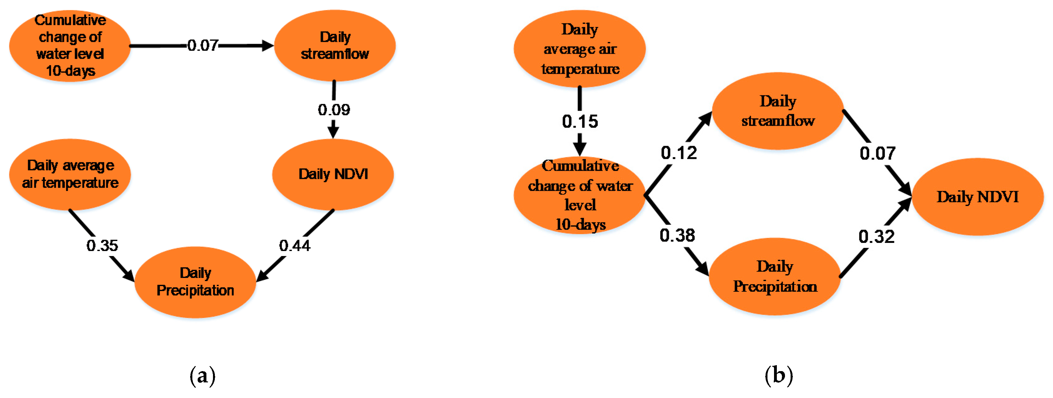
As Figure 2 shows, the observed causal networks of the Yichang and Beipei stations were constructed. For the Yichang station, we find two prominent causal linkages in Figure 2a. One linkage is between the daily NDVI and the daily precipitation, the score of which was 0.44. The other is the linkage between the daily average air temperature (DAAT) and the daily precipitation, the score of which was 0.35. The results showed that the daily NDVI is driving most precipitation variability in Yichang station. The results are in accordance with the hypothesis that precipitation intensities will increase with temperature according to the Clausius–Clapyeron relation, a warmer atmosphere being capable of holding more moisture [31]. We also observed a linkage path from the cumulative change of water level (CCOWL) to the daily streamflow. For example, the MOHID-Land model always provides unrealistic estimates in the hydrometric stations located upstream of the reservoir management without considering the discovered linkage. A weak evidence of causality for the daily streamflow to the daily NDVI was found. This was highly relevant regarding the fact that the NDVI dynamics were highly correlated with other metrological factors, such as soil moisture, as reported in [32]. The results also indicated that the CCOWL indirectly drives the vegetation dynamics at the Yichang station. For the Beipei station, we find two prominent causal linkages in Figure 2b: one linkage is between the daily precipitation and the daily NDVI, the score of which was 0.32; the other is the linkage between the 10 days CCOWL and the daily precipitation, the score of which was 0.38. The results showed that the 10 days CCOWL was driving the daily precipitation dynamics at the Beipei station. As compared with the direction of the linkage between the daily NDVI and the daily precipitation of Yichang station, the direction of the same linkage of Beipei station is from the daily precipitation to the daily NDVI. The result showed that there is bidirectional causality between the daily NDVI and daily precipitation in these regions. Our finding confirms that the ecological protections project designed to protect vegetation has greatly changed the natural vegetation landscape. The ecological restoration projects conducted in the local region of the TGRA exert a positive impact on vegetation greening as reported in [33]. The results also suggested that the TGR regulations induced the change in precipitation and was likely an important factor driving the precipitation changes at the Beipei stations. Because Beipei is in the Buffer-50 km that is a region further away from the TGRA, we presume that the TGR regulations would influence the vegetation dynamics on the wider region. We did not observe any linkage between 20 days CCOWL and other variables, or the linkage between 30 days CCOWL and other variables. The reason was likely that the cumulative water level changes of a longer period would influence the vegetation dynamics across a wider area, which will be investigated in the next section.
4.2. Explainable Variances of NDVI with Respect to the Water Level
To understand the spatial–temporal model of the explored causality relations, we investigated the water level–vegetation dynamics conditioned by climate variables (specifically including precipitation and air temperature in the experiments). We used the aforementioned non-linear causality framework to investigate the relations across the five regions. In the following experiments, the number of trees used were 2000 and the maximum number of features per node was set automatically for the random forest regressor. We used 10-fold cross-validation to prevent over fitting and set the maximum depth of the trees of the random forests to 20. Considering the adaption of the plant to the climate variations and human activities naturally require some time, we used the cumulative sum of the water level and lagged air temperature and precipitation as the predictor variables. To obtain stationary time series, we used the anomaly decomposition and seasonality-detrending methods described in [13].
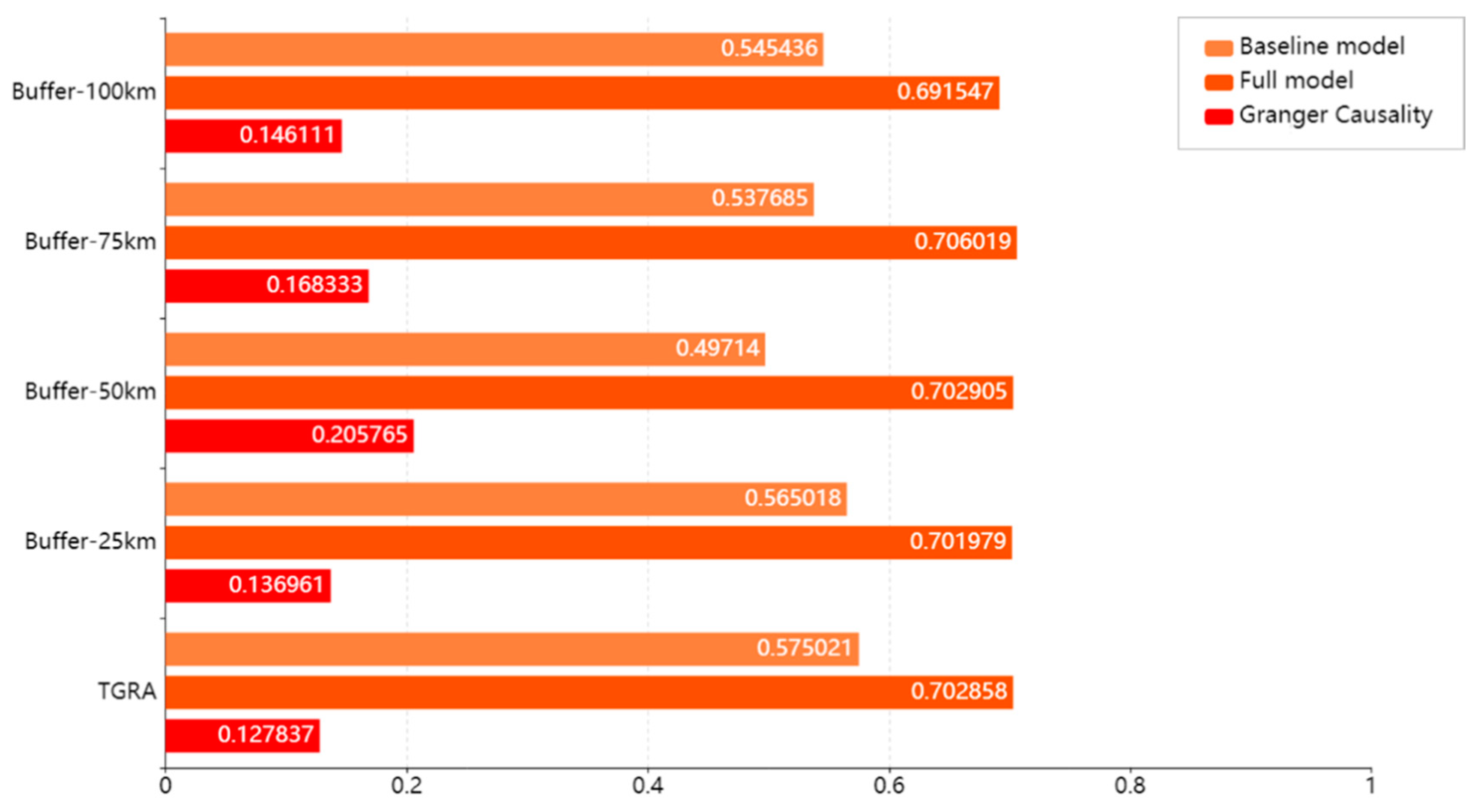
We investigated the causalities between the cumulative sum of water level and the vegetation response across the study area. Formally, we constructed the cumulative variable of k days as the sum of the time series of the water level in the last k days. We derived the cumulative variable to incorporate the potential impact of the TGR water resources scheduling on the vegetation dynamics in the study area. Based on the indirect linkages between 10 days CCOWL and the daily NDVI obtained, we conducted the following experiments considering the different cumulative periods (). According to the non-linear GC, the full model represents the cumulated sum of the last k day’s water level, and the lagged climate variables are predictors. The baseline model represents only past values of NDVI and the lagged climate variables are included as predictors. Note that the lagged time windows were the same as the cumulative periods. The response variable was the daily NDVI, which is the same for both the full model and the baseline model. The non-linear GC represents the improvement of the coefficient of determination by subtracting the predication accuracy from the full model with respect to that of the baseline model. Figure 3 shows the results of the feedbacks of vegetation with respect to the cumulative sum of the water level (CSWL) in the study area. The GCs of the five regions range from 0.127 to 0.205. The results showed that the 10 days CSWL of the TGR could explain the vegetation variance up to 20.5% in these regions. With the increase in distance between the metrological stations and TGR, GCs increase from 0.1278 to 0.2057. GCs decrease from 0.2057 to 0.1461 when the distance from the stations to the TGR increase above 75 km. The GC of stations in the TGRA is the weakest, which is highly correlated with the complex and rugged topography of the region that could easily affect the vegetation dynamic [33]. The implementation of forestry ecological projects led to afforestation as reported in [34]. The result also suggested that the water resources scheduling would influence on the regional scale, which correspond with Wu’s research. The causality between the CSWL and the daily NDVI is at the regional scale rather than the local scale.
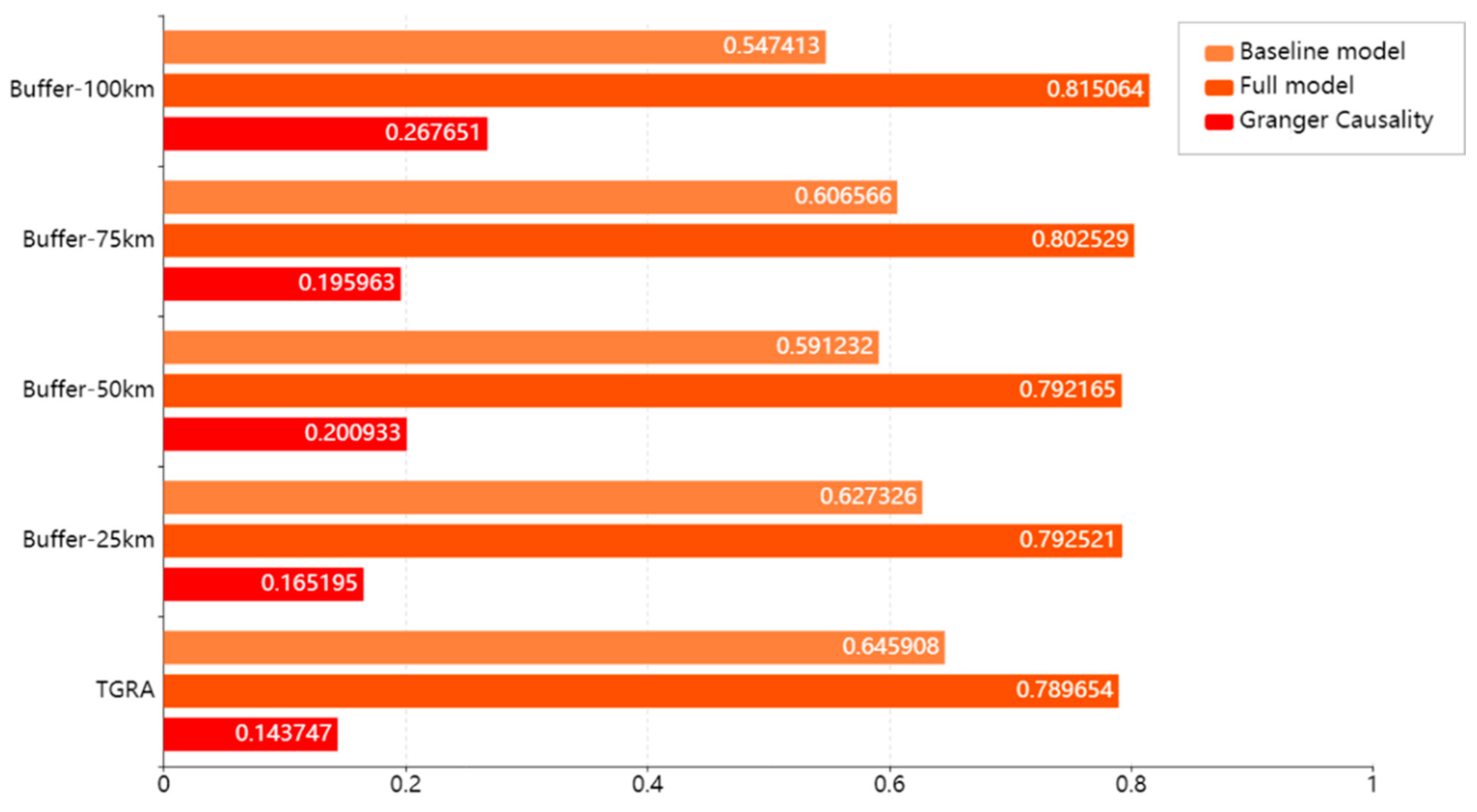
Figure 4 shows the results of vegetation dynamics response to the cumulated sum of 20 days’ water level in the study area. The GCs of the five regions range from 0.14 to 0.26. With the increase in distance between the metrological stations and the TGR, GCs increase from 0.1437 to 0.2676. The results suggested that the water level variation Granger cause the vegetation growth with a median factor of 19.46% across the study area. Now that the frequency of the TGR operation is nearly in the quarter scale, our finding suggested that the fine-grained water regulation scale would beneficial for boosting the vegetation growth. In addition to the finding, we observed that the prediction accuracy of the baseline model is rather high in this context. With the increase in distance between the metrological stations and TGR, the coefficient of determination of the random forest model decreased from 0.64 to 0.54. The results demonstrated that the lagged variations of precipitation and air temperature would be highly correlated with the vegetation phenology. The results indicated that the vegetation changes were highly correlated with the lagged climate impact.
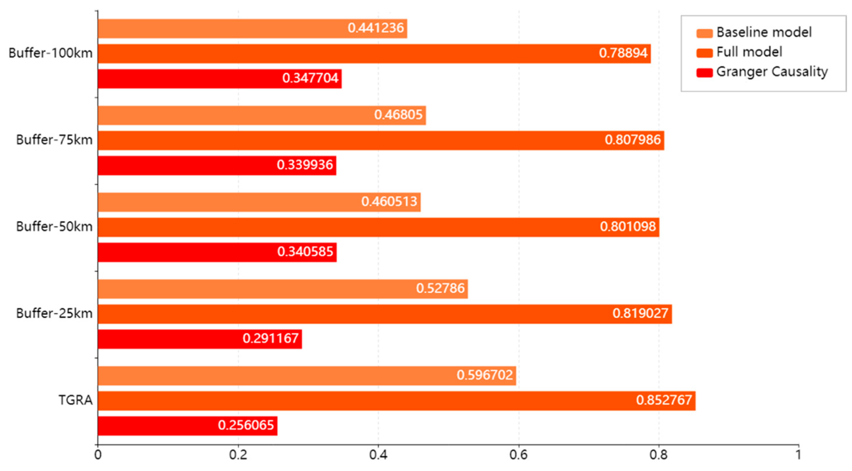
Figure 5 shows the results of vegetation dynamics response to the 30 days CSWL. The GCs of the five regions range from 0.25 to 0.34. With the increase in distance between the metrological stations and TGR, the GCs of the stations increase from 0.2560 to 0.3477. The results showed that 30 days CSWL significantly causes the NDVI changes in the 100 km area. The results confirm the finding that fine-grained TGR operations would be beneficial for vegetation coverage restoration in the study area. TGR operation at the monthly scale may be better for boosting the ecological restoration process. The climate variables are the dominant factors that influence the vegetation phenology; we find that the causality between the 30 days CSWL and the vegetation dynamics is also prominent. We also observed that the coefficient of determinations of the baseline models decrease from 0.59 to 0.44. Still, the results indicated that the water level regulation is another import factor for improving the vegetation status in the 10km buffer region.
4.3. Spatial–Temporal Granger Causality across TGRA
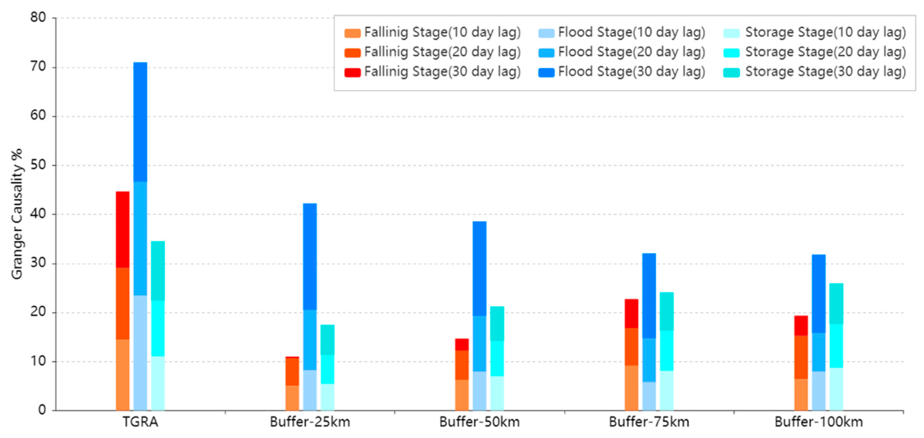
We investigated the spatial–temporal causality of the vegetation dynamics to the water level variations across the study area. The spatial extent contains five buffers regions. The temporal scope includes the falling stage, the flood stage and the storage stage of the TGR operation of the baseline year. We used the daily air temperature and precipitation from 2006 to 2015 in the following experiments. The parameters of the non-linear GC were the same as used earlier. The difference between the following experiments and the above experiments is that we used the lagged water level as the predictors instead of the cumulative sum of the water level. As seen in Figure 6, the percentages of the 10 days lagged water level with Granger causality to NDVI of the falling stage in the TGRA, buffer-25 km, buffer-50 km, buffer-75 km and buffer-100 km are 14.42%, 5%, 6.32%, 9.1% and 6.39% respectively. The percentages of the 20 days lagged water level with Granger causality to NDVI of the falling stage in the TGRA, buffer-25 km, buffer-50 km, buffer-75 km and buffer-100 km are 14.65%, 5.73%, 5.95%, 7.73% and 8.83% respectively. The percentages of the 30 days lagged water level with Granger causality to NDVI of the falling stage in the TGRA, buffer-25 km, buffer-50 km, buffer-75 km and buffer-100 km are 15.63%, 0.3%, 2.42%, 5.93% and 4.15% respectively. From our finding, it can be inferred that the TGR operation in the falling stage can greatly improve the vegetation growth in the TGRA. The results of the 10 days lagged water level Granger causality vegetation dynamics in the TGRA are consistent with our earlier result as shown in Figure 3. Regarding the TGR regulation in the flood season, the percentages of the 10 days lagged water level with Granger causality to NDVI of the flood stage in the TGRA, buffer-25 km, buffer-50 km, buffer-75 km and buffer-100 km are 23.49%, 8.2%, 7.92%, 5.79% and 7.98% respectively. The percentages of the 20 days lagged water level with Granger causality to NDVI of the flood stage in the TGRA, buffer-25 km, buffer-50 km, buffer-75 km and buffer-100 km are 23.13%, 12.3%, 11.4%, 8.97%, and 7.8% respectively. The percentages of the 30 days lagged water level with Granger causality to NDVI of the flood stage in the TGRA, buffer-25 km, buffer-50 km, buffer-75 km and buffer-100 km are 24.38%, 21.72%, 19.24%, 17.31% and 16.03% respectively. The results suggested that the TGR operation in the flood stage could significantly improve the vegetation growth in the TGRA. Moreover, we observed that the 30 days lagged water level can significantly improve the vegetation growth in the flood season for the entire study area. This finding is important in that ecological restoration activity can be feasibly conducted during the flood season. Regarding the TGR regulation in the storage season, the percentages of the 10 days lagged water level with Granger causality to NDVI of the storage stage in the TGRA, buffer-25 km, buffer-50 km, buffer-75 km and buffer-100 km are 11.06%, 5.4%, 7.01%, 8.1% and 8.7% respectively. The percentages of the 20 days lagged water level with Granger causality to NDVI of the storage stage in the TGRA, buffer-25 km, buffer-50 km, buffer-75 km and buffer-100 km are 11.39%, 5.97%, 7.19%, 8.2% and 8.93% respectively. The percentages of the 30 days lagged water level with Granger causality to NDVI of the storage stage in the TGRA, buffer-25 km, buffer-50 km, buffer-75 km and buffer-100 km are 12.05%, 6.13%, 7.01%, 7.81% and 8.3% respectively. From our finding, it can be inferred that the TGR operation in the storage stage has limited influence on the vegetation growth in the study area. This was highly correlated with the vegetation that ceased to grow in that period.
5. Discussion and Conclusions
In this study, the spatial–temporal causality between water level and the vegetation dynamics was investigated. We used an approach that combines the CGNNs with a non-linear Granger-causality framework. From 10 years of daily water level and remotely sensed NDVI from the MODIS09GA product, we found that the 30-days water level fluctuation significantly changes the vegetation phenology of the region with a median factor of 31.5% in the 100 km region. The results showed that the vegetation dynamics linked to the water level regulation are of regional scale rather than of the local scale. We found that water level regulation in the flood stage can greatly improve the vegetation growth in the buffer regions of the TGRA. Specifically, the explainable Granger causalities of the 25 km buffer region, 50 km buffer region, 75 km buffer region and 100km buffer regions are 21.72%, 19.24%, 17.31% and 16.03%, respectively. Although in the falling stage and impounding stage, where the functionality of the TGR that boost the vegetation growth was not obvious (qualified value ranges from 6.1% to 8.3%), our results demonstrated the regional vegetation dynamics of the TGD were driven not only by the factor of climate changes but also by anthropogenic influence, which was rarely mentioned in previous studies. Moreover, our findings are useful for policymakers to design fine-grained water scheduling strategies to support the ecological restoration projects that were highlighted in recent years.
The analysis procedure consisted of four parts. In the first part, the results of the MK tests showed that the coupling effect of the TGR operation with climate variations boosted the vegetation growth in the TGRA. In the second part, the deep-learning-based causality inference model facilitated unsupervised feature selections and discovered the prominent linkages without any data preprocessing. In the third and fourth parts, the non-linear causality framework was used to quantify the linkages formally. All of the time series features used for the causality inference procedure were tested with the Augmented Dickey–Fuller Test to maintain the stationary requirement. However, we think some aspects would require further study. First, only two meteorological station were used in the deep-learning model, because of the limitation in the availability of the daily streamflow data. Second, the CGNNs were not considering the temporal and spatial aspect, which require tentative methods to investigate the time-lagged impacts among the features. Finally, we did not consider the soil moisture–atmosphere feedback that can influence the precipitation [8]. However, the construction of the CGNNs as shown in Figure 2 has considered the streamflow instead. The potential confounding factors would also include atmospheric humidity and radiation, which were not considered in the water–climate–plant feedbacks in this study. The paucity of these datasets may restrict the conclusions to some extent. We will consider possible negative effects in the downstream part of the basins due to fluvial segmentation [35] and droughts [36] in future work.
Author Contributions
Conceptualization, D.Z. and W.H.; methodology, W.H.; validation, D.Z. and W.H.; formal analysis, W.H.; data curation, D.Z. and W.H.; writing—original draft preparation, W.H.; writing—review and editing, D.Z. and J.Z.; visualization, D.Z. and W.H.; supervision, J.Z.; project administration, J.Z.; funding acquisition, J.Z. All authors have read and agreed to the published version of the manuscript.
Funding
This research was funded by the National Natural Science Foundation of China: Risk assessment and runoff adaptive utilization in water resource system considering the complex relationship among water supply, electricity generation, and environment (grant number 91547208).
Acknowledgments
The authors greatly appreciate the anonymous reviewers and academic editor for their careful comments and valuable suggestions to improve the manuscript.
Conflicts of Interest
The authors declare no conflict of interest.
References
- Zheng, T.; Qiang, M.; Chen, W.; Xia, B.; Wang, J. An externality evaluation model for hydropower projects: A case study of the Three Gorges Project. Energy 2016, 108, 74–85. [Google Scholar] [CrossRef]
- Han, X.; Feng, L.; Hu, C.; Chen, X. Wetland changes of China’s largest freshwater lake and their linkage with the Three Gorges Dam. Remote Sens. Environ. 2018, 204, 799–811. [Google Scholar] [CrossRef]
- Mei, X.; Dai, Z.; Du, J.; Chen, J. Linkage between Three Gorges Dam impacts and the dramatic recessions in China’s largest freshwater lake, Poyang Lake. Sci. Rep. 2015, 5, 18197. [Google Scholar] [CrossRef] [Green Version]
- Wang, J.; Sheng, Y.; Wada, Y. Little impact of the Three Gorges Dam on recent decadal lake decline across China’s Yangtze Plain. Water Resour. Res. 2017, 53, 3854–3877. [Google Scholar] [CrossRef] [Green Version]
- Qu, S.; Wang, L.; Lin, A.; Zhu, H.; Yuan, M. What drives the vegetation restoration in Yangtze River basin, China: Climate change or anthropogenic factors? Ecol. Indic. 2018, 90, 438–450. [Google Scholar] [CrossRef]
- Zhao, Y.; Zou, X.; Liu, Q.; Yao, Y.; Li, Y.; Wu, X.; Wang, C.; Yu, W.; Wang, T. Assessing natural and anthropogenic influences on water discharge and sediment load in the Yangtze River, China. Sci. Total. Environ. 2017, 607, 920–932. [Google Scholar] [CrossRef]
- Sridhar, V.; Kang, H.; Ali, S. Human-Induced Alterations to Land Use and Climate and Their Responses for Hydrology and Water Management in the Mekong River Basin. Water 2019, 11, 1307. [Google Scholar] [CrossRef] [Green Version]
- Jaksa, W.T.; Sridhar, V. Effect of irrigation in simulating long-term evapotranspiration climatology in a human-dominated river basin system. Agric. For. Meteorol. 2015, 200, 109–118. [Google Scholar] [CrossRef]
- Reichenbach, H. The Direction of Time; Univ of California Press: Berkeley, CA, USA, 1991; Volume 65. [Google Scholar]
- Runge, J.; Bathiany, S.; Bollt, E.; Camps-Valls, G.; Coumou, D.; Deyle, E.; Glymour, C.; Kretschmer, M.; Mahecha, M.; Muñoz-Marí, J.; et al. Inferring causation from time series in Earth system sciences. Nat. Commun. 2019, 10, 2553. [Google Scholar] [CrossRef] [PubMed]
- Perez-Suay, A.; Camps-Valls, G. Causal Inference in Geoscience and Remote Sensing From Observational Data. IEEE Trans. Geosci. Remote. Sens. 2018, 57, 1502–1513. [Google Scholar] [CrossRef]
- Green, J.K.; Konings, A.; Alemohammad, H.; Berry, J.; Entekhabi, D.; Kolassa, J.; Lee, J.-E.; Gentine, P. Regionally strong feedbacks between the atmosphere and terrestrial biosphere. Nat. Geosci. 2017, 10, 410–414. [Google Scholar] [CrossRef] [PubMed]
- Papagiannopoulou, C.; Miralles, D.G.; Decubber, S.; Demuzere, M.; Verhoest, N.; Dorigo, W.A.; Waegeman, W. A non-linear Granger-causality framework to investigate climate–vegetation dynamics. Geosci. Model Dev. 2017, 10, 1945–1960. [Google Scholar] [CrossRef] [Green Version]
- Song, Z.; Liang, S.; Feng, L.; He, T.; Song, X.-P.; Zhang, L. Temperature changes in Three Gorges Reservoir Area and linkage with Three Gorges Project. J. Geophys. Res. Atmos. 2017, 122, 4866–4879. [Google Scholar] [CrossRef]
- Chai, Y.; Li, Y.; Yang, Y.; Zhu, B.; Li, S.; Xu, C.; Liu, C. Influence of Climate Variability and Reservoir Operation on Streamflow in the Yangtze River. Sci. Rep. 2019, 9, 5060. [Google Scholar] [CrossRef] [PubMed]
- Wu, L.; Zhang, Q.; Jiang, Z. Three Gorges Dam affects regional precipitation. Geophys. Res. Lett. 2006, 33, 33. [Google Scholar] [CrossRef] [Green Version]
- Bao, Y.; Gao, P.; He, X. The water-level fluctuation zone of Three Gorges Reservoir—A unique geomorphological unit. Earth-Sci. Rev. 2015, 150, 14–24. [Google Scholar] [CrossRef]
- Tang, H.; Wasowski, J.; Juang, C.H. Geohazards in the three Gorges Reservoir Area, China–Lessons learned from decades of research. Eng. Geol. 2019, 261, 105267. [Google Scholar] [CrossRef]
- Qin, P.; Xu, H.; Liu, M.; Du, L.; Xiao, C.; Liu, L.; Tarroja, B. Climate change impacts on Three Gorges Reservoir impoundment and hydropower generation. J. Hydrol. 2020, 580, 123922. [Google Scholar] [CrossRef]
- Chen, C.; Park, T.; Wang, X.; Piao, S.; Xu, B.; Chaturvedi, R.K.; Fuchs, R.; Brovkin, V.; Ciais, P.; Fensholt, R.; et al. China and India lead in greening of the world through land-use management. Nat. Sustain. 2019, 2, 122–129. [Google Scholar] [CrossRef]
- Gocic, M.; Trajkovic, S. Analysis of changes in meteorological variables using Mann-Kendall and Sen’s slope estimator statistical tests in Serbia. Globa. Planet. Chang. 2013, 100, 172–182. [Google Scholar] [CrossRef]
- Goudet, O.; Kalainathan, D.; Caillou, P.; Guyon, I.; Lopez-Paz, D.; Sebag, M. Causal generative neural networks. arXiv 2017, 1711, 08936. [Google Scholar]
- Neuberg, L.G. Causality: Models, Reasoning, and Inference, by Judea Pearl; Cambridge University Press: Cambridge, UK, 2003; Volume 19, pp. 675–685. [Google Scholar]
- Earl, D.C. Ronald Syme, Sallust. University of California Press/Cambridge University Press, 1964. Pp. viii + 381. 50s. J. Rom. Stud. 1965, 55, 232–240. [Google Scholar] [CrossRef]
- Carlier, G.; Chernozhukov, V.; Galichon, A. Vector quantile regression: An optimal transport approach. Ann. Stat. 2016, 44, 1165–1192. [Google Scholar] [CrossRef]
- Chickering, D.M. Optimal structure identification with greedy search. J. Mach. Learn. Res. 2002, 3, 507–554. [Google Scholar]
- Gretton, A.; Borgwardt, K.; Rasch, M.J.; Scholkopf, B.; Smola, A.J. A Kernel Method for the Two-Sample Problem. arXiv 2008, 0805, 2368. [Google Scholar]
- Yamada, M.; Jitkrittum, W.; Sigal, L.; Xing, E.P.; Sugiyama, M. High-Dimensional Feature Selection by Feature-Wise Kernelized Lasso. Neural Comput. 2014, 26, 185–207. [Google Scholar] [CrossRef] [PubMed] [Green Version]
- Dickey, D.A.; Fuller, W.A. Distribution of the estimators for autoregressive time series with a unit root. J. AM. Stat. Assoc. 1979, 74, 427–431. [Google Scholar]
- Wu, Z.; Huang, N.E.; Long, S.R.; Peng, C.-K. On the trend, detrending, and variability of nonlinear and nonstationary time series. Proc. Natl. Acad. Sci. USA 2007, 104, 14889–14894. [Google Scholar] [CrossRef] [Green Version]
- Blenkinsop, S.; Chan, S.C.; Kendon, E.J.; Roberts, N.M.; Fowler, H. Temperature influences on intense UK hourly precipitation and dependency on large-scale circulation. Environ. Res. Lett. 2015, 10, 54021. [Google Scholar] [CrossRef] [Green Version]
- Zhang, H.; Chang, J.; Zhang, L.; Wang, Y.; Li, Y.; Wang, X. NDVI dynamic changes and their relationship with meteorological factors and soil moisture. Environ. Earth Sci. 2018, 77, 582. [Google Scholar] [CrossRef]
- Wen, Z.; Wu, S.; Chen, J.; Lü, M. NDVI indicated long-term interannual changes in vegetation activities and their responses to climatic and anthropogenic factors in the Three Gorges Reservoir Region, China. Sci. Total. Environ. 2017, 574, 947–959. [Google Scholar] [CrossRef] [PubMed]
- Huang, C.; Huang, X.; Peng, C.; Zhou, Z.; Teng, M.; Wang, P. Land use/cover change in the Three Gorges Reservoir area, China: Reconciling the land use conflicts between development and protection. Catena 2019, 175, 388–399. [Google Scholar] [CrossRef]
- Dai, Z.; Liu, J. Impacts of large dams on downstream fluvial sedimentation: An example of the Three Gorges Dam (TGD) on the Changjiang (Yangtze River). J. Hydrol. 2013, 480, 10–18. [Google Scholar] [CrossRef]
- Li, S.; Xiong, L.; Dong, L.; Zhang, J.J.H.P. Effects of the Three Gorges Reservoir on the hydrological droughts at the downstream Yichang station during 2003–2011. Hydrol. Process. 2013, 27, 3981–3993. [Google Scholar] [CrossRef]
Figure 1.
The study area across the Three George Reservoir area (TGRA). The inner most is the TGRA containing 21 meteorological stations. The other four buffering regions are depicted using different colors. The thick blue line depicts the Yangtze River and the thin blue lines depict the branches of the Yangtze River.

Figure 2.
A deep-learning-based causal network inference method applied on the time series data of the Yichang and Beipei stations (preserving prominent causality linkages only). (a) Observed data causal network of the Yichang station (b) Observed data causal network of the Beipei station.
Figure 2.
A deep-learning-based causal network inference method applied on the time series data of the Yichang and Beipei stations (preserving prominent causality linkages only). (a) Observed data causal network of the Yichang station (b) Observed data causal network of the Beipei station.

Figure 3.
Feedbacks of vegetation dynamics with respect to the cumulative sum of 10 days’ water level.
Figure 3.
Feedbacks of vegetation dynamics with respect to the cumulative sum of 10 days’ water level.

Figure 4.
Feedbacks of vegetation dynamics with respect to the cumulative sum of 20 days’ water level.
Figure 4.
Feedbacks of vegetation dynamics with respect to the cumulative sum of 20 days’ water level.

Figure 5.
Feedbacks of vegetation dynamics with respect to the cumulative sum of 30 days’ water level.
Figure 5.
Feedbacks of vegetation dynamics with respect to the cumulative sum of 30 days’ water level.

Figure 6.
The spatial–temporal causality for the vegetation dynamics due to the water level variations across the TGRA.
Figure 6.
The spatial–temporal causality for the vegetation dynamics due to the water level variations across the TGRA.

© 2020 by the authors. Licensee MDPI, Basel, Switzerland. This article is an open access article distributed under the terms and conditions of the Creative Commons Attribution (CC BY) license (http://creativecommons.org/licenses/by/4.0/).
Share and Cite
MDPI and ACS Style
Huang, W.; Zhou, J.; Zhang, D. Exploring Empirical Linkage of Water Level–Climate–Vegetation across the Three Georges Dam Areas. Water 2020, 12, 965. https://doi.org/10.3390/w12040965
AMA Style
Huang W, Zhou J, Zhang D. Exploring Empirical Linkage of Water Level–Climate–Vegetation across the Three Georges Dam Areas. Water. 2020; 12(4):965. https://doi.org/10.3390/w12040965
Chicago/Turabian StyleHuang, Wei, Jianzhong Zhou, and Dongying Zhang. 2020. "Exploring Empirical Linkage of Water Level–Climate–Vegetation across the Three Georges Dam Areas" Water 12, no. 4: 965. https://doi.org/10.3390/w12040965
Note that from the first issue of 2016, this journal uses article numbers instead of page numbers. See further details here.