Three-Dimensional Flow Characteristics in Slit-Type Permeable Spur Dike Fields: Efficacy in Riverbank Protection

Abstract

This paper focuses on finding efficient solutions for the design of a highly permeable pile spur (or slit type) dike field used in morphologically dynamic alluvial rivers. To test the suitability of different arrangements of this type of permeable pile spur dike field, laboratory experiments were conducted, and a three-dimensional multiphase numerical model was developed and applied, based on the experimental conditions. Three different angles to the approach flow and two types of individual pile position arrangements were tested. The results show that by using a series of slit-type spurs, the approach velocity of the flow can be considerably reduced within the spur dike zone. Using different sets of angles and installation positions, this type of permeable spur dike can be used more efficiently than traditional dikes. Notably, this type of spur dike can reduce the longitudinal velocity, turbulence intensity, and bed shear stress in the near-bank area. Additionally, the deflection of the permeable spur produces more transverse flow to the opposite bank. Arranging the piles in staggered grid positions among different spurs in a spur dike field improves functionality in terms of creating a quasi-uniform turbulence zone while simultaneously reducing the bed shear stress. Finally, the efficacy of the slit-type permeable spur dike field as a solution to the riverbank erosion problem is numerically tested in a reach of a braided river, the Brahmaputra–Jamuna River, and a comparison is made with a conventional spur dike field. The results indicate that the proposed structure ensures the smooth passing of flow compared with that for the conventional impermeable spur structure by producing a lower level of scouring (low bed shear stress) and flow intensification.

1. Introduction

Riverbank erosion is considered one of the major issues in the deltaic regions of the world, especially in the Ganges–Brahmaputra–Meghna (GBM) delta region, from which more than sixty thousand people migrate each year due to riverbank erosion [1,2]. Among the deltaic rivers in the GBM region, the sand bed-braided Brahmaputra–Jamuna River erodes five hundred meters per year [2]. The rapid change in braided channel geometry triggers variations in the flow boundary conditions and the hydraulic structures, and changes are considered the key management issues for dynamic alluvial rivers worldwide, particularly the Brahmaputra–Jamuna River [3,4]. Several countermeasures are generally used to protect the river banks, e.g., revetment with rip rap made of different materials and the establishment of hardpoints (heavy-duty embankments) and permeable and impermeable spurs [4,5]. Previous studies have shown that almost all types of structures are partly or totally damaged when exposed to the main channel [6]. However, spur-type structures experienced frequent and severe damage compared to other high-cost river training structures, e.g., long embankments, due to the dynamic characteristics of the river and instability of the flows (governed by local scouring) induced by the structures [6,7]. Around the world, previous studies documented the use of spur dikes in rivers to provide adequate depth, mitigate bank erosion, and improve land reclamation and ecological richness by creating stagnant zones [4,6,8,9,10,11,12,13,14,15,16,17,18]. However, field observations and multiple laboratory studies have revealed relatively large scour holes produced by impermeable spur dike fields. Angled flows, bedform movement, and rapid siltation or erosion downstream create favorable conditions for local scouring [7,8,16,17,18,19,20,21,22,23] Therefore, a detailed understanding of the flow around such structures is crucial for the optimum design of spur dikes to manage this type of dynamic river.

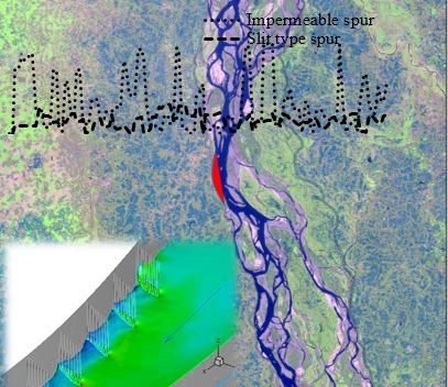
As an alternate solution, permeable spur dikes that produce less severe morphological consequences have become popular in India, Bangladesh, the United States of America (USA), and the Netherlands, among other countries [10,24,25]. Although this type of spur dike is reported to work very well in some rivers, the performance is questionable in large rivers [6]. Figure 1a shows an example of a failed semipermeable spur dike in the Brahmaputra–Jamuna River in Bangladesh, Figure 1b shows the initial spur constructed approximately 500 m from the main channel in 2013, and Figure 1c illustrates the reinforced cement concrete (RCC) part of the dike, which is completely immersed when the river flows through the main channel at certain times. Figure 1c also shows the flow pattern of the river. The authors surveyed the velocity of the river near the structure (500 m downstream) and upstream (12 km) of the structure (Figure 1c shows the survey points), using an acoustic Doppler current profiler (ADCP) (Figure 1d). Figure 1d gives no indication of very high flow velocities near the structure, but the structure still failed. A previous study [4] analyzed the failure cases of different types of structures in this river and found that the transverse flow generated due to spur-type structures has the potential to create local scouring, which is frequently ignored during dike design. The local vortex at the structure tip also plays a significant role in creating local scour. This type of failure indicates an improper understanding of the flow field around a spur dike. These circumstances are the motivation for this research.

We propose a highly permeable slit-type pile spur dike field (permeability > 70%; the width of the individual pile is small relative to the channel width, and the channel width/pile width ratio is 200) to overcome the aforementioned issues by decreasing the impact on the riverbed. As the first step in our research, we performed a laboratory experiment and numerical simulations to understand the three-dimensional flow properties around this type of structure. Then, a successful alignment was numerically tested for a reach of the Brahmaputra River.

Although many experimental and numerical studies have been conducted to examine the mean flow properties around impermeable spurs [9,10,19,26,27,28], relatively few studies have examined permeable cases [11,17,18,24,29,30,31].

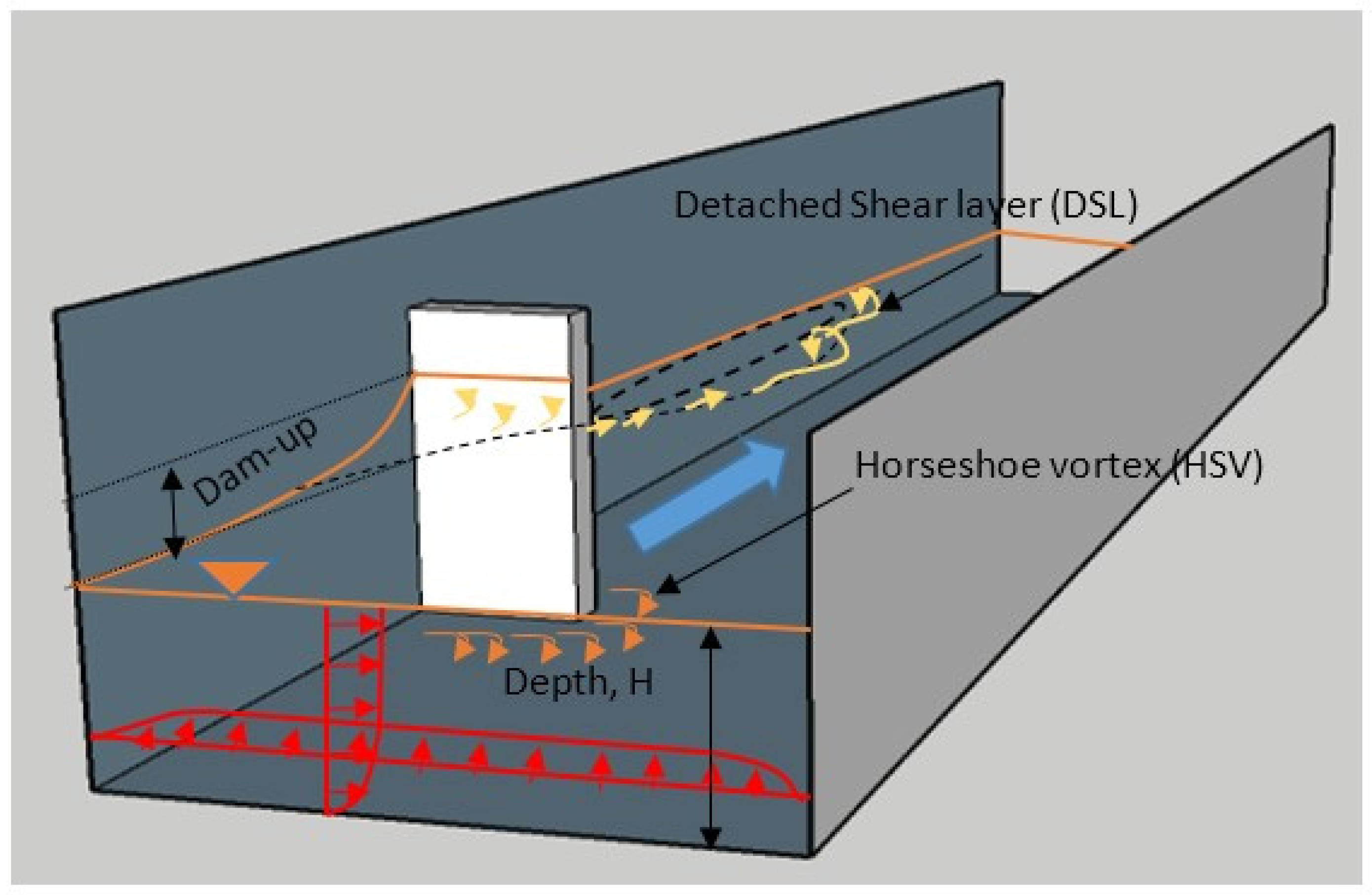
The flow around the spur dike (see Figure 2) is relatively complex due to the adverse pressure gradient immediately upstream of the spur dike, a quasi-periodic recirculation zone, the formation of a horseshoe vortex (HSV) system at the base of the spur dike, the development of a wake zone, a fully turbulent and dynamic detached shear layer (DSL), and vortex shedding at the tip of the spur dike [32,33,34]. These phenomena, particularly the HSV system, accelerated flow at the tip, and the DSL produce a large shear stress and turbulence at the spur tip, which may undermine a spur in an alluvial river by producing large scour holes [35,36,37]. In a spur dike field, the eroded material deposited further downstream increases the channel roughness. To successfully design a spur dike field, knowledge of the combined effects of these phenomena is crucial. However, most of the previous work focused on the flow field, bed scouring, and three-dimensional turbulent features of impermeable spur dikes, and less is known about the flow features around permeable spur dikes.

Some researchers [38] investigated a permeable pile groin in the Baltic Sea and reported its efficiency at reducing the turbulence intensity at the bed and improving large-scale recirculation. Others [39] investigated a permeable groin by considering vegetation as a permeable groin and focused on determining the corresponding effects on flood control and the environment. Certain researchers [40] examined permeable spurs as rubble-mound structures using laboratory experiments and a two-dimensional model focusing on the rubble geometry of a group of groins in terms of the flow structure and the flow force. A study [41] examined the three-dimensional flow features around a porous spur dike by developing a three-dimensional analytical model using the k-ε model of turbulence and found some discrepancies downstream of the spur dike. Another study [17] used a laboratory experiment to compare suspended sediment transport in permeable and impermeable spur dike fields and concluded that the suspended sediment concentration decreases in the downstream direction due to sedimentation in the transition zone for permeable spur dikes; they used a staggered group of poles as an individual spur dike. Researchers [18] examined the effect of permeability on a single spur based on laboratory experimentation and recommended an appropriate permeability to reduce the velocity at the groin tip. In summary, the definition of a permeable spur dike differs throughout the literature, and there are few studies on pile spur dike fields.

Hence, the main objective of this research was to identify the three-dimensional flow behavior around a series of slit-type spur dike fields with different installation arrangements. The specific objective was to find the optimal solution for this type of spur dike in terms of the installation angle and spur position through experimentation and numerical simulations. In addition, we investigated the efficacy of this type of structure for riverbank protection. For this purpose, six experimental cases were investigated; these cases are described in later sections of the paper. The numerical simulation was performed by solving the three-dimensional Reynolds-averaged Navier–Stokes (RANS) equations, considering multiphase flow and using the $k-\omega$ SST model of turbulence. We hypothesized that a better understanding of the flow phenomena around this type of structure will be helpful for understanding the flow patterns of similar geometrical structures. Finally, the appropriate solutions were tested in a small river reach.

2. Laboratory Experiment

To understand the flow around a slit-type spur dike field, experiments were performed under fixed-bed conditions at Ujigawa Open Laboratory, Kyoto University. A movable bed may provide a better understanding of the scouring process near spur dikes, but the flow depth of movable beds can vary around spur dikes, and the appropriate procedures to accurately measure the adjusted flow dam-up are ambiguous. In contrast, with a fixed bed, it is straightforward to measure the flow depth or dam-up variation and the three-dimensional velocity at multiple depths. Therefore, as a first step, experiments were performed using a fixed-bed condition. The flume was 10 m long and 0.8 m wide with a longitudinal slope of 1/300. The details of the experimental configuration are shown in

Table 1. Experimental case details.

Cases	Angle to the u/s Flow (Degree)	Installation Arrangement	Number of Spur Dikes	Number of Piles in Each Spur Dike
1	90	Squared	5	13
2	90	Staggered	5	13
3	120	Squared	5	15
4	120	Staggered	5	15
5	60	Squared	5	15
6	60	Staggered	5	15

and Figure 3.

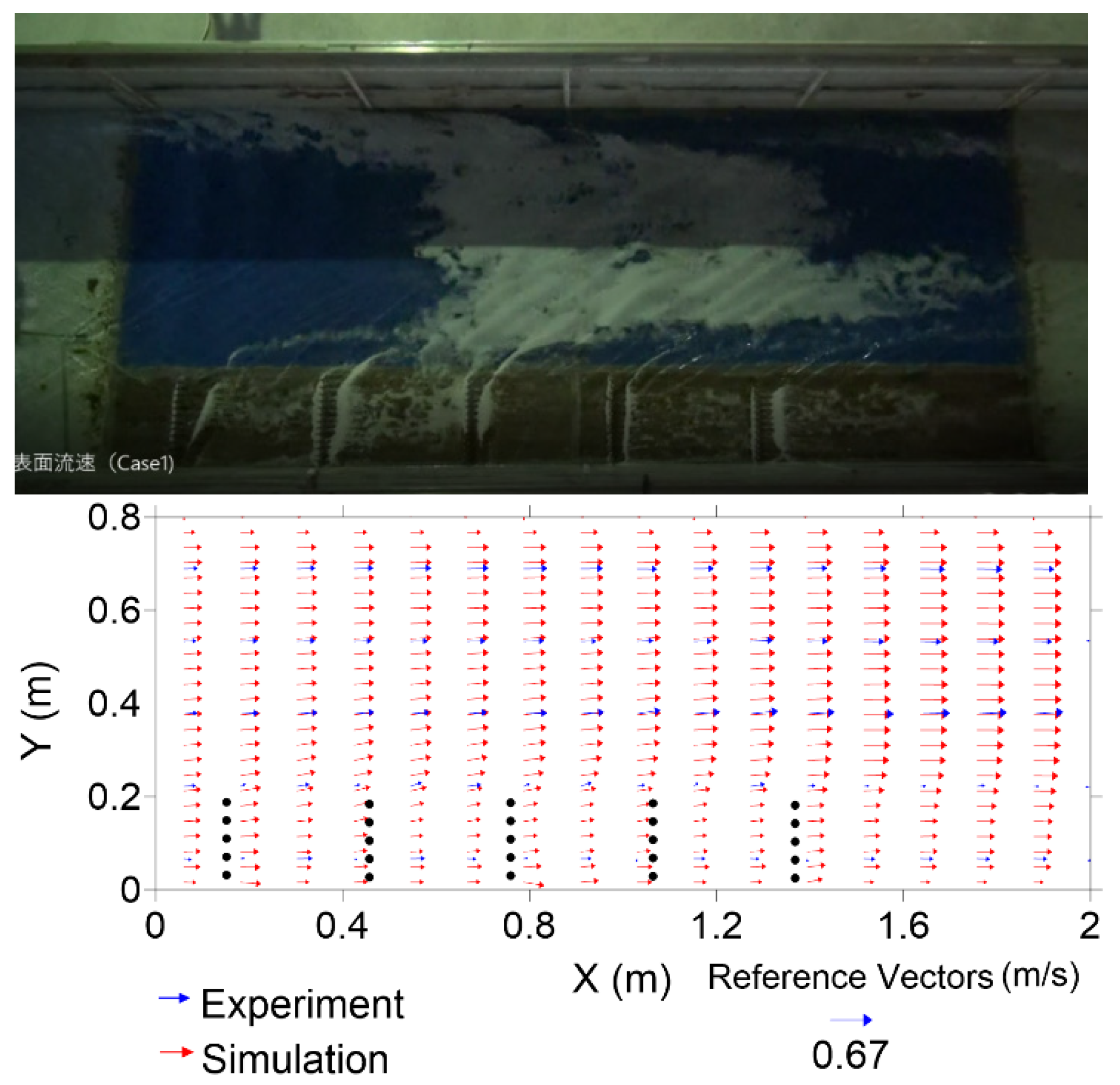
Figure 3a–c describes the plan and sections of the flume. Figure 3d shows a photograph of the flume for case 1. A continuous discharge of 0.01 m³/s was supplied from the upstream region. The five spur dikes were installed 7 m from the upstream end of the right bank. Each spur dike consisted of cylindrical brass piles with diameters of 0.004 m. The spacing between two individual piles was 0.001 m, and the longitudinal interval of each was 0.30 m. A total of five spur dikes were installed, each with a permeability of 71%. Two types of installations were considered: a squared grid-type pile setting and a staggered grid-type pile setting (Figure 3e). The approach flow depth was 0.032 m, and uniform flow was confirmed by adjusting the flume-end weir height. The details of the hydraulic conditions of the flume are described in

Table 2. Experimental Conditions.

Parameter	Unit	Values
Discharge, Q	m3/s	0.01
Channel slope, s	-	1/300
Channel width, W	m	0.80
Approach flow depth, h	m	0.032
Approach flow velocity, U	m/s	0.40
Friction velocity, $U_{*}$	m/s	0.0323
Reynolds number, R	-	34,430
Froude number, F	-	0.71
Approach flow bed shear stress, τo	N/m2	1.0464
Manning’s n	s/m1/3	0.015

.

The water depth was measured using an OMRON ultrasonic water level sensor (accuracy $\pm 0.001 m$), and the particle image velocimetry (PIV) method was used to measure the surface flow velocity. Model ACM250-A, JFE Alec Co., Ltd.’s L-type electromagnetic velocity meter was used to measure the three-dimensional velocity ($\underset{\_}{u}, \underset{\_}{v},\underset{\_}{w}$) components (accuracy $\pm 0.005 m/s$). All types of velocity data were measured at depths of Z = 0.01 m and Z = 0.02 m from the bottom. Longitudinal velocity $\underset{\_}{u},\underset{\_}{w}$ data were gathered 0.117 m from the right bank at a distance of 0.02 m from each individual spur and at the midpoint of two consecutive spurs (0.152 m away). The transverse velocity ($\underset{\_}{v},\underset{\_}{w}$) and water depth were measured 0.02 m from each spur at the same projected perpendicular location from the right bank. In addition, the flow depth was measured at mid-channel (0.40 m from the right bank of channel).

3. Numerical Simulation

3.1. Governing Equations

The numerical model was based on the three-dimensional RANS equations for a free surface, as shown in Equations (1) and (2):

$$\nabla .U=0$$

(1)

$$\frac{\partial \rho U}{\partial t}+\nabla .\left(\rho UU\right)=-\nabla p+\nabla .\tau +\rho g+\rho f_{\alpha }$$

(2)

Here, Equation (2) consists of the time-dependent and convective terms of the velocity on the left side, whereas the viscosity and the external forces are on the right. The stress tensor is obtained from the molecular and turbulent viscosities and given by Equation (3):

$$\tau ={\mu }_m\left(\nabla U+{\left(\nabla U\right)}^T\right)+\rho R$$

(3)

In the RANS model, the Reynolds decomposition of the velocity $U$ into its mean $\underset{\_}{u}$ and fluctuating contribution $\acute{u}$ was obtained as shown in Equation (4):

$$U\left(x,t\right)=\underset{\_}{u}\left(x,t\right)+\acute{u}\left(x,t\right)$$

(4)

where the mean of the fluctuating component is defined as zero; i.e., $\underset{\_}{\acute{u}}=0$. The Reynolds stress tensor $R$ is obtained from the fluctuating velocity component using Equation (5):

$$R=\underset{\_}{\acute{u}\acute{u}}$$

(5)

Based on the Boussinesq eddy viscosity assumption, the momentum transfer caused by turbulent eddies was modeled with an eddy viscosity term, and the momentum transfer caused by the molecular motion can be described by the molecular viscosity. The Reynolds stress tensor is further divided into isotropic and deviatoric anisotropic contributions using Equation (6):

$$R=\frac{2}{3}kI+R_{dev}$$

(6)

$R_{dev}$ can be obtained using Equation (7). Only the anisotropic contribution, $R_{dev}$, of the Reynolds stress tensor transports momentum (in Equation (2)), and the isotropic contribution, $\frac{2}{3}kI$, is added to the mean pressure.

$$R_{dev}={\vartheta }_t\left(\nabla U+{\left(\nabla U\right)}^T\right)-\frac{2}{3}kI$$

(7)

The $k-\omega$ SST model [42,43,44] was applied for turbulence closure. Such turbulence model is chosen because of its well predictions in adverse pressure gradients and separating flow [44]. The turbulent kinetic energy, $k$, the specific dissipation rate, $\omega$, and the turbulent kinematic eddy viscosity, ${\vartheta }_t$, were calculated by using Equations (8)–(10):

$$\frac{\partial \left(\rho k\right)}{\partial t}+\rho \left[\nabla .\left(kU\right)\right]=S_k-{\beta }^{*}\rho k\omega +\nabla \left[\left(\mu +{\alpha }_k{\vartheta }_t\right)\nabla \left(\rho k\right)\right]$$

(8)

$$\frac{\partial \left(\rho \omega \right)}{\partial t}+\rho \left[\nabla .\left(\omega U\right)\right]=S_w-\beta \rho {\omega }^2+\nabla \left[\left(\vartheta +{\alpha }_k{\vartheta }_t\right)\nabla \left(\rho \omega \right)\right]+\left(1-F_1\right)\rho C{D}_{\omega }$$

(9)

$${\vartheta }_t=\frac{a_{1}k}{\left(a_1\omega ,S{F}_2\right) }$$

(10)

where

$$S_k=\left(G_k,c_1\rho {\beta }^{*}k\omega \right)$$

(11)

$$G_k={\vartheta }_t{S}^2$$

(12)

$$S_w=\frac{\gamma }{{\vartheta }_t}{G}_k$$

(13)

$$C{D}_w=2{\alpha }_{\omega 2}\frac{1}{\omega }\nabla k\nabla \omega$$

(14)

$F_1$$F_1$ = 0 in the free stream and $F_1$ $F_1$ = 1 at any wall boundary. ${\alpha }_{k1},{\alpha }_{k2}, {\alpha }_{\omega 2},{\beta }^{*}, \beta \gamma ,c_1, and a_1{\alpha }_{k1},{\alpha }_{k2}, {\alpha }_{\omega 2},{\beta }^{*}, \beta \gamma ,c_1,a_1$ are the turbulent model coefficient constants shown in

Table 3. $k-\omega$ SST model constants.

${\mathit{\alpha }}_{\mathit{k}1}$	${\mathit{\alpha }}_{\mathit{k}2}$	${\mathit{\alpha }}_{\mathit{\omega }1}$	${\mathit{\alpha }}_{\mathit{\omega }2}$	${\mathit{\beta }}^{*}$	$\mathit{\beta }$	$\mathit{\gamma }$	${\mathit{c}}_1$	${\mathit{a}}_1$
0.85	1.0	0.5	0.856	0.9	0.075	0.5532	10	0.31

.

$$F_1=tanh tanh \left[{\left(min\left\{min\left(\left(\frac{\sqrt{k}}{{\beta }^{*}\omega y},\frac{500\vartheta }{y^2\omega }\right),\frac{4{\alpha }_{\omega 2}k}{C{D}_{k\omega }^{+}{y}^2} \right),10\right\}\right)}^4\right]$$

(15)

$$F_2=tanh tanh \left[{\left\{min\left(max\left(\frac{2\sqrt{k}}{{\beta }^{*}\omega y},\frac{500\vartheta }{y^2\omega }\right),100\right)\right\}}^2\right]$$

(16)

where

$$C{D}_{k\omega }^{+}=max\left(C{D}_{k\omega },1e^{-10}\right)$$

(17)

$${\alpha }_k={\alpha }_{k1}{F}_1+{\alpha }_{k2}{F}_2$$

(18)

The volume of fluid (VOF) method was used to capture the free surface flow, as described previously [45]. Therefore, along with the continuity and momentum equations, another transport equation (Equation (19)) that represents the volume fraction of one phase is solved simultaneously with these equations.

$$\frac{d\alpha }{dt}+\nabla .\left(\alpha U\right)=0$$

(19)

The phase fraction, $\alpha$, ranges from 0 ≤$\alpha \le$ 1, e.g., $\alpha$ = 0 for air and $\alpha$ = 1 for water. The free surface was assumed to have a volume fraction of 0.5. As air and water are considered two immiscible fluids, the physical properties of fluids are calculated based on the weighted average distribution of the liquid volume fraction. For example, the density of each cell, $\rho$, was calculated using Equation (20).

$$\rho ={\rho }_a\alpha +\left(1-\alpha \right){\rho }_w$$

(20)

where ${\rho }_a and {\rho }_w$ denote density of air and water respectively. In Equation (1), $f_{\alpha }$ represents the surface tension effects at the free surface, and this variable is calculated by using Equations (21) and (22).

$$f_{\alpha }={\sigma }_T{k}_{\alpha }\nabla \alpha$$

(21)

$$k_{\alpha }=-\nabla .\left(\frac{\nabla \alpha }{\left|\nabla \alpha \right|}\right)$$

(22)

Here, $k_{\alpha }$ is the curvature of the interface and ${\sigma }_T$ is surface tension. However, in free surface simulations, mass conservation should be confirmed in each phase and for the given surface curvature, which is required for the determination of the surface tension and the pressure gradient across free surface [46]. Therefore, to ensure the mass conservation of the phase fraction, a modified transport equation is solved, as proposed in [47] and shown in Equation (23).

$$\frac{d\alpha }{dt}+\nabla .\left(\alpha U\right)+\nabla .\alpha U_r\left(1-\alpha \right)=0$$

(23)

Here, $U_r$ is the relative velocity, which can be expressed as $U_r=U_f-U_a$. The additional convective term in Equation (23) is named the compression term, and it makes an artificial contribution to convection to make the free surface sharper [48]. The term contains a nonzero value within the interface region and hence has no influence in single-phase regions. The PIMPLE algorithm, which is a combination of the pressure implicit with the splitting of the operator (PISO) method and semi-implicit method for pressure-linked equations (SIMPLE) method, was used to couple the pressure and momentum quantities. The PIMPLE algorithm was chosen due to its stability and use of a larger time step compared to those of the PISO and SIMPLE algorithms. Numerical analysis was performed using the open-source interFoam solver within the open-source OpenFOAM platform.

3.2. Model Schematization

A hybrid mesh consisting of quadrangles and prisms was used in the simulations. An example computation is shown in Figure 4. Five domain patches were considered: the inlet, outlet, bed, atmosphere, and wall (including spur dikes). The simulation conditions were kept the same as the experimental conditions.

Table 4. Boundary conditions of the simulations.

Domain Patch	Velocity, U	Pressure, $\mathit{p}$	Turbulent Kinetic Energy, k	Specific Dissipation Rate, ω	Turbulent Kinematic Eddy Viscosity, ${\mathit{\vartheta }}_{\mathit{t}}$	Phase Fraction, α
Inlet	variableHeightFlowRateInletVelocity i	zero gradient	Uniform fixed value	Uniform fixed value	Uniform fixed value	variableHeightFlowRate
Outlet	pressureInletOutletVelocity ii	totalPressure iii	internalField	Uniform fixed value	Calculated from other patch fields	inletOutlet iv
Walls	noSlip	zero gradient	kqRWallFunction	omegaWallFunction	nutUSpaldingWallFunction	zero gradient
Atmosphere	pressureInletOutletVelocity	totalPressure	uniform fixed value	inletOutlet	Calculated from other patch fields	inletOutlet
Bed	noSlip	zero gradient	kqRWallFunction	omegaWallFunction	nutUSpaldingWallFunction	zero gradient

ⁱ Velocity was estimated by using $U_{avg}=\frac{Q}{{\alpha }_1.S}$. ⁱⁱ When p is known at the inlet, U was evaluated from the flux normal to the patch. ⁱⁱⁱ The patch pressure was estimated from $p=p_0-\frac{1}{2}\left|U\right|$. ^iv The outflow condition was generic (zero gradient), with a specified inflow for the case of a return flow.

shows the boundary conditions used in the simulations for all cases. A detailed description and definitions of the boundary types can be found in previous reports [49,50,51]. The calculation conditions were the same as those in the experiments; a variable-height velocity induced by the 0.01 m³/s supply of discharge upstream was given at the inlet (variableHeightFlowRateInletVelocity), enabling free water level oscillation (variableHeightFlowRate) and a constant total pressure at the outlet $\left(p_0\right)$. A no-slip condition was applied to the walls as a velocity boundary condition. The upper surfaces of the mesh were considered to correspond to the atmosphere; therefore, flow was allowed to enter and leave the domain freely by applying the pressureInletOutletVelocity condition for velocity and the totalPressure condition for pressure. The wall function approach was used to link the turbulent flow domains near the wall-like structures. kqRWallFunction, omegaWallFunction, and nutUSpaldingWallFunction were applied to the walls as the turbulent boundary conditions. A mesh convergence analysis has been done by the author to some extent (considering the study mesh and 50% refinement of study mesh in all directions) and the author found no significant change in water depth and velocity component.

3.3. Validation of the Flow Hydrodynamics

In the computational fluid dynamics (CFD), the validation of the numerical model or calculation is a fundamental step for the acceptability of the code as described by previous researchers [52,53,54]. They [52,53] discussed the importance of quantification of uncertainty in CFD methods and recommended that, despite having uncertainty in estimation for both numerical modeling and experiments, at least scaled experiments are adequate for model validation [53]. Later other researchers i.e., [54] extended the CFD best practice guidelines and concluded that the definition and conceptualization of the system along with prior knowledge are necessary as the initial steps of CFD modeling. Nevertheless, the selection of model features and parameter values and evaluation of the model performance are necessary for the best practice in CFD modeling. In light with these, the definition and conceptualization of the system of this research is described in Section 1. Section 2 and Section 3 discuss the model features and parameter values and the validation of the model is discussed in the following paragraphs.

Here, the numerical simulations were validated with the measured experimental data. A comparison of the surface velocity values derived using the PIV method and the simulation of case 1 is shown in Figure 5.

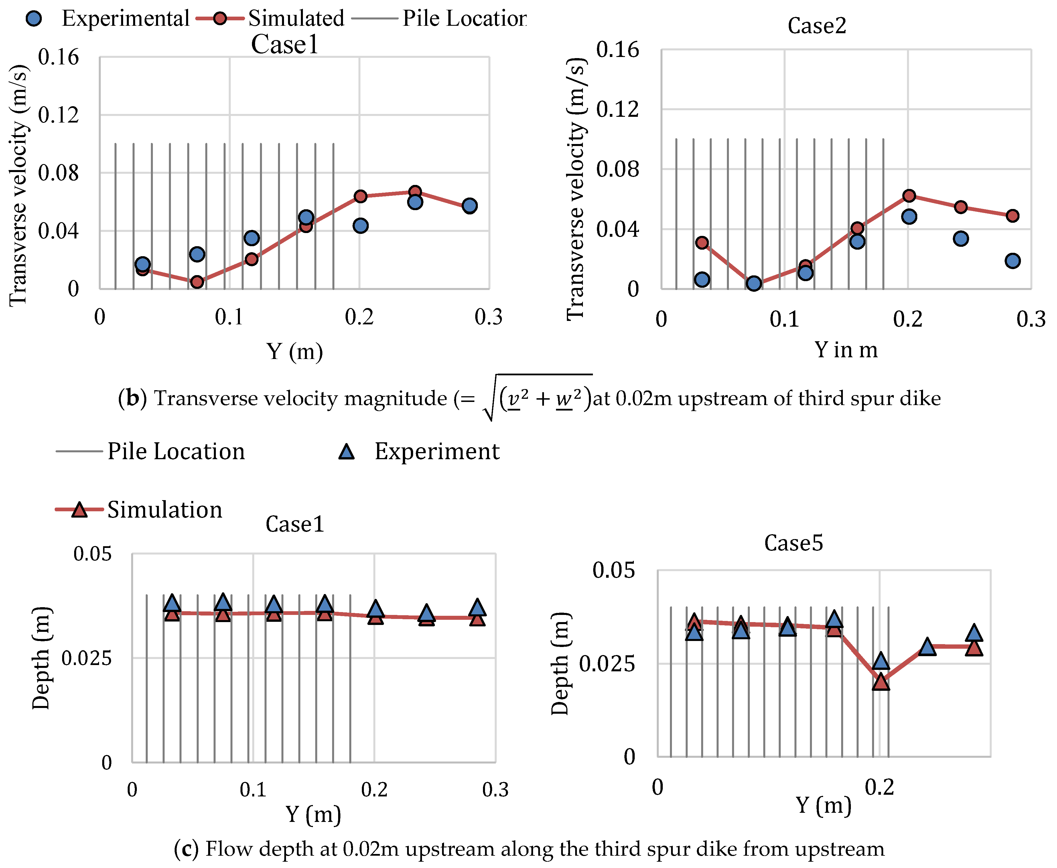
In addition, comparisons of the three-dimensional velocity ($\underset{\_}{u},\underset{\_}{v},\underset{\_}{w}$) and water depth were made for each data measurement location; a typical example is shown in Figure 6.

Despite some differences, a comparison of these values reflects satisfactory agreement between the two cases. The model performance was assessed using Equation (24), and the Percent bias (PBIAS) values at all measurement points for the water depth and velocity are shown in

Table 5. Percent bias (PBIAS) of the considered cases.

Cases	PBIAS (%)
	Water Depth	Velocity Magnitude
Case 1	−5.06	−11.05
Case 2	3.31	−18.12
Case 3	1.33	−15.92
Case 4	8.76	3.79
Case 5	9.83	8.68
Case 6	11.82	−6.27

.

$$PBIAS=\left(\frac{{\sum }_{i=1}^n{S}_i-{\sum }_{i=1}^n{O}_i}{{\sum }_{i=1}^n{O}_i}\right)\times 100$$

(24)

Previous research [51,55,56] reported a satisfactory range for PBIAS of $0\le PBIAS\le 25\%.$ Table 5 indicates that all the cases discussed here are within this acceptable range. However, in the simulation, RANS equations were used, which give approximate time-averaged solutions for the flow parameters. Thus, the experimental results may display a trend similar to that of the simulation results. Comparing the longitudinal and transverse velocity in Figure 6, it can be noted that the numerical model seemed to predict higher value in case of transverse velocity. The transverse velocity is generally affected by the coherent turbulent structure generated around the spurs. The results indicated limitation in capturing such turbulent structure when using RANS equations. However, for the water depth, the simulation result was underestimated in case 1 but slightly overestimated (maximum 11.8%) in the other cases. The velocity magnitude results of the simulations were overestimated in cases 4 and 5 but underestimated in the other cases (maximum 18.1%). It should be noted that PBIAS indicates the average tendency of the simulated data to be greater or smaller than the experimental data [57].

4. Results and Discussion

The experimental results were nondimensionalized by dividing the respective field value by the approach flow depth h and approach flow velocity U.

4.1. Longitudinal Velocity

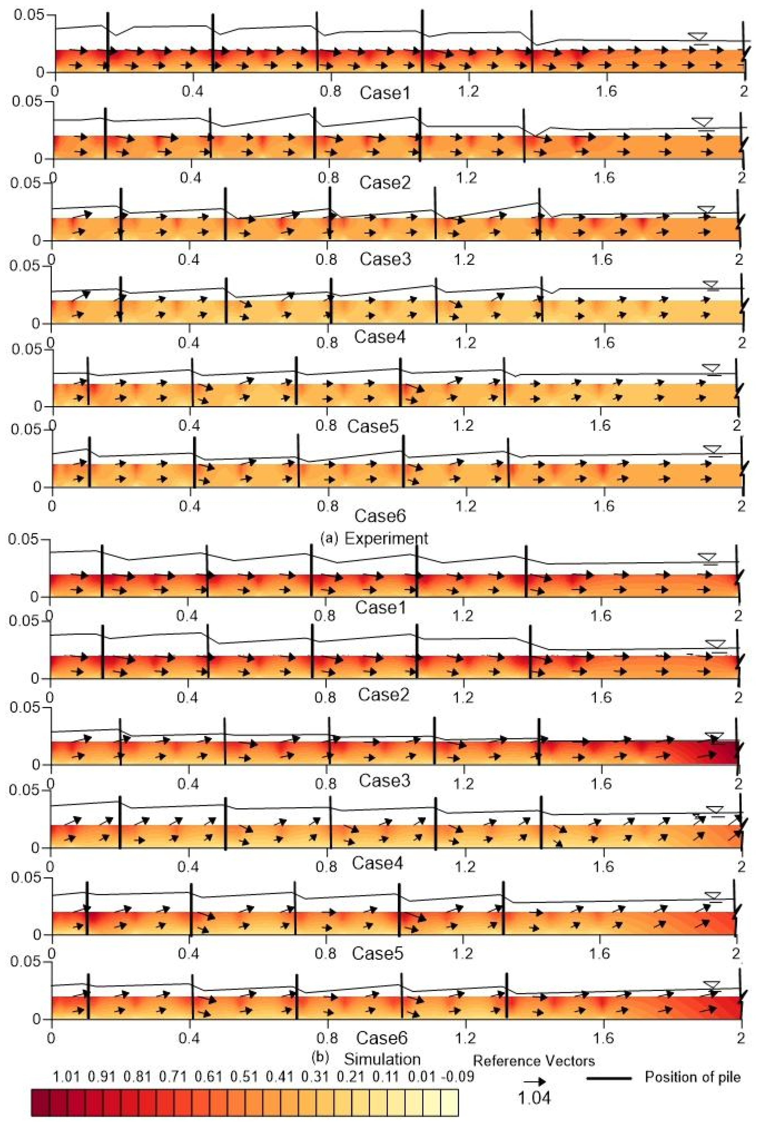
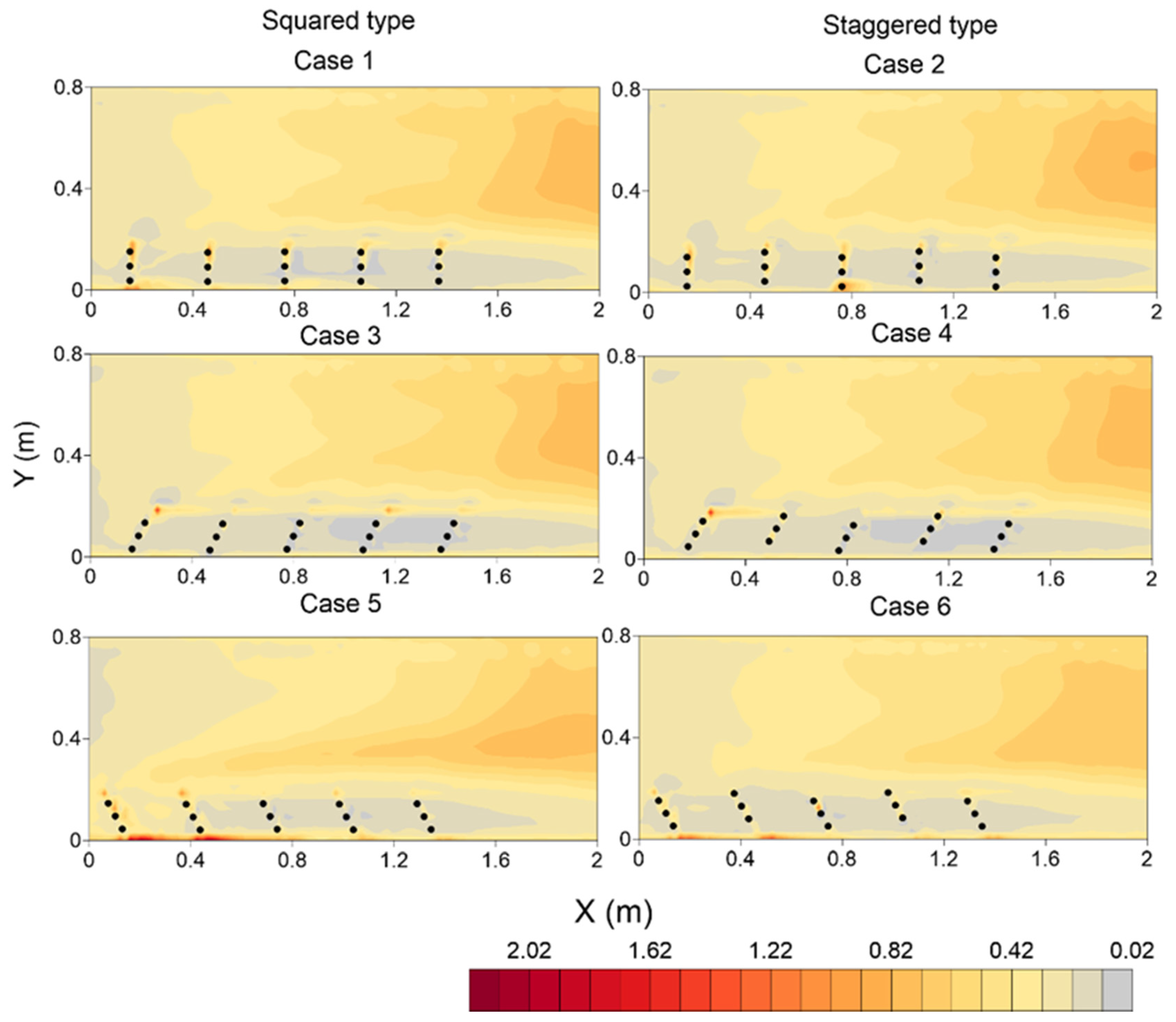
Figure 7 shows the variation in the dimensionless longitudinal velocity vectors $\left(\frac{\underset{\_}{u}}{U},\frac{\underset{\_}{w}}{U}\right)$ at a distance of 0.11 m from the right bank. The top Figure 7a show the results of the experiments, and the bottom Figure 7b show the results of the simulations. Satisfactory matching for both the magnitude and patterns of the longitudinal vectors is observed. These figures indicate that the magnitude of the longitudinal velocity $\left(\frac{\underset{\_}{u}}{U}\right)$ vector varies from −0.09 to 1.1 within the spur dike zone. All the cases confirmed that the downward component became stronger just after passing the spur dike. However, as the permeability of the spur dikes was relatively high, no strong recirculating flow was observed. This observation is similar to those noted previously [17,18]. Researchers [18] found no recirculation when the permeability was greater than 60%. The maximum average magnitude of $\frac{\underset{\_}{u}}{U}$ occurred in case 1 (experimental: average = 0.88, maximum = 1.07; simulated: average = 0.79, maximum = 1.08). The minimum average magnitude of $\frac{\underset{\_}{u}}{U}$ occurred in case 4 (experimental: average = 0.56, maximum = 0.70; simulated: average = 0.7, maximum = 0.85). In almost all cases, the square installation had an almost 6% higher longitudinal velocity in both the simulation and experiment. The strongest vertical component $\frac{\underset{\_}{w}}{U}$ was found in case 4. Within the spur dike zone, in the perpendicular (case 1 and case 2) and deflecting (case 5 and case 6) cases, both the experimental and simulated cases confirmed that the highest longitudinal velocity was observed around the first spur dike in the upstream region. However, for cases 3 and 4, the location of the highest longitudinal velocity was different; for case 3, it was found 0.02 m downstream of the fifth spur dike, and for case 4, it was found 0.02 m upstream of the first spur dike. This difference arose due to the different installation positions.

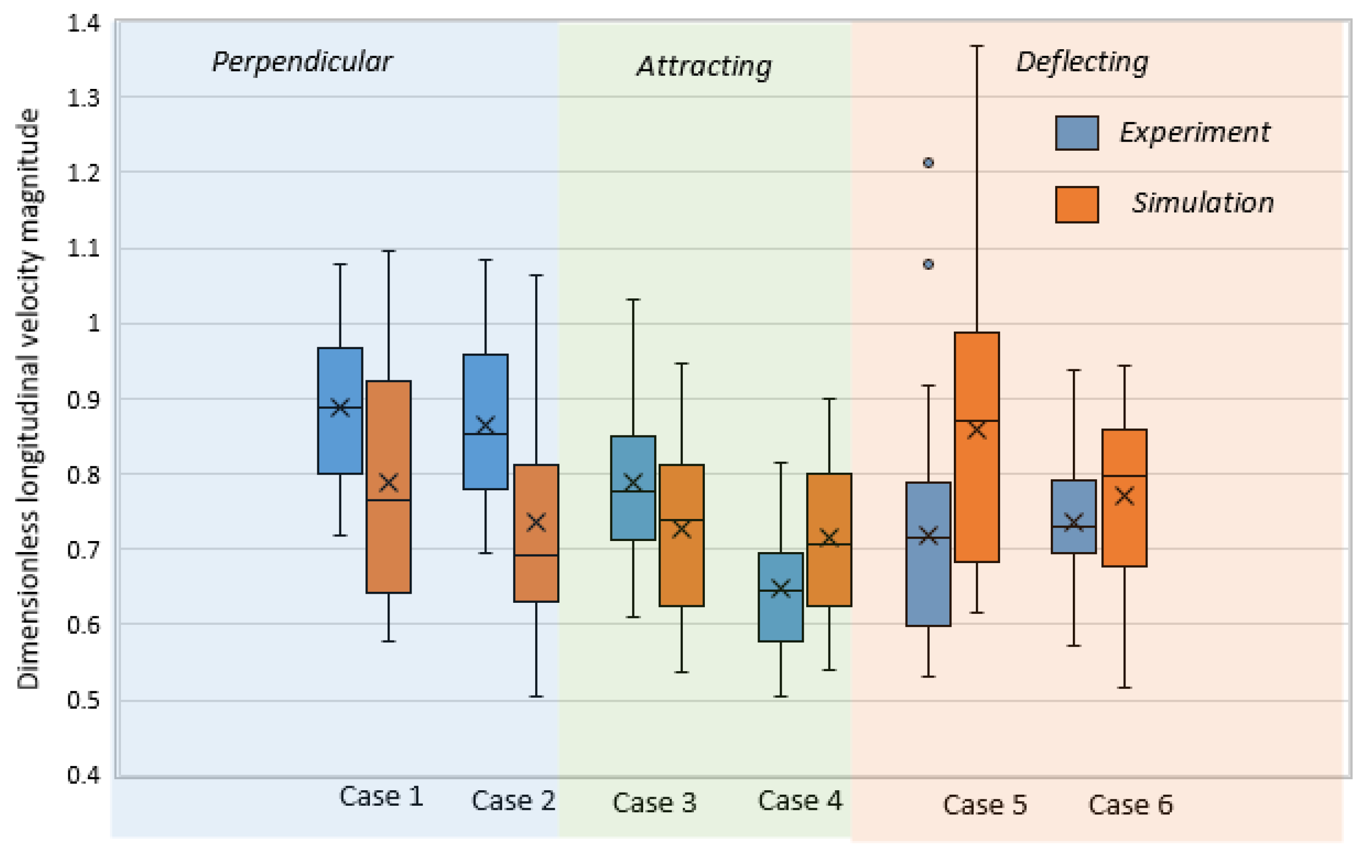
Figure 8 shows a boxplot of the magnitude of the longitudinal velocity. This figure shows a similar tendency for all cases except experimental case 5 and case 6, which have similar mean values (0.79). In experimental case 5, the data have a wide range, including two outlier points. Additionally, the simulation results confirm that the longitudinal velocity was higher in case 5 than in other cases. The average magnitude of the dimensionless longitudinal velocity within the spur dike field was 0.77 (over all cases).

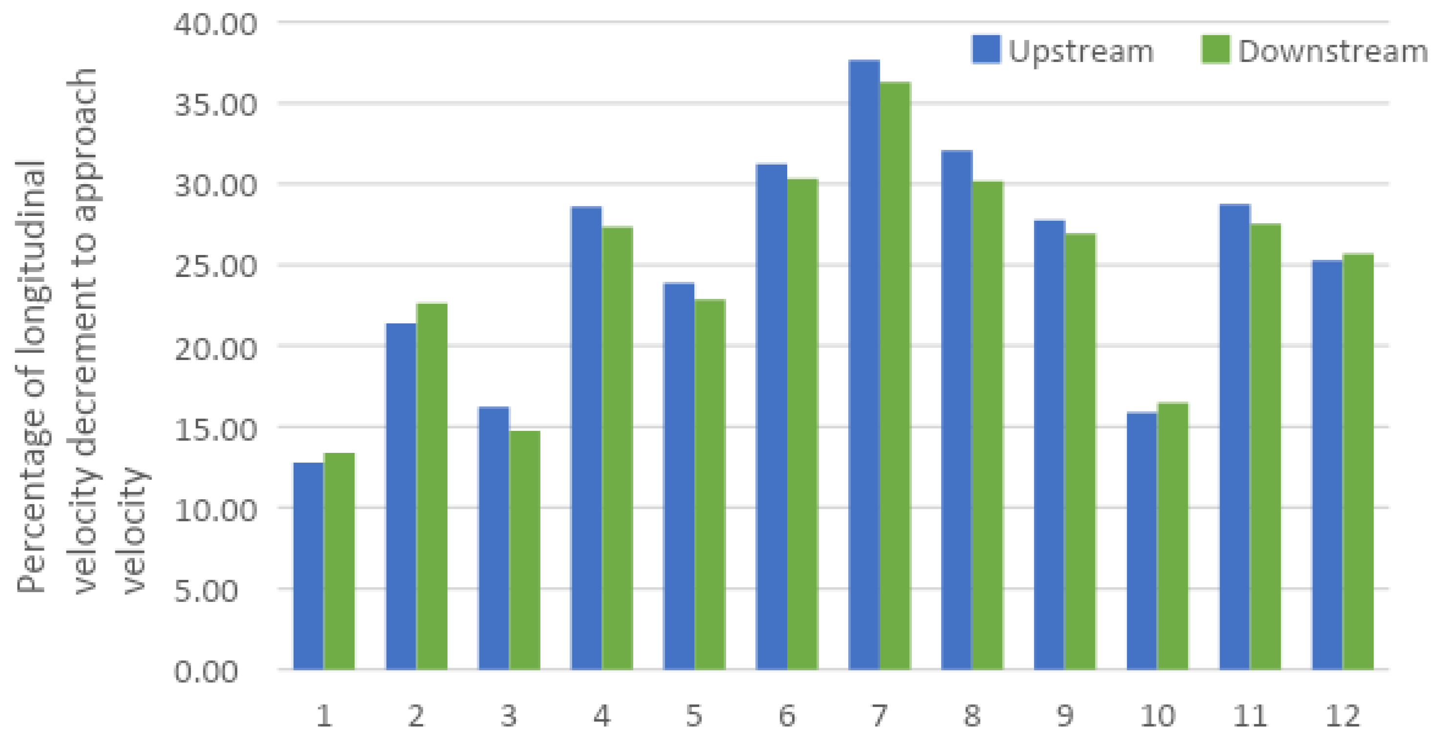
Figure 9 shows the average ratio of the velocity decrease to the approach velocity 0.02 m upstream and 0.02 m downstream of each spur dike. This type of permeable structure can reduce the approach velocity by almost 25%. In addition, the highest possible longitudinal velocity reduction (over 30%) near a spur dike occurred for the attracting type of spur dike (case 3 and case 4). Moreover, the staggered installation yielded the lowest velocity just upstream and downstream of the spur dike (case 4).

4.2. Transverse Velocity

Figure 10 shows the variation in the nondimensional transverse velocity vector 0.02 m upstream of the third spur dike; (a) shows the experimental results, and (b) shows the simulated results. This figure indicates that the magnitude of the dimensionless transverse velocity $\left(\frac{\underset{\_}{v}}{U}\right)$ ranges from −0.035 to 0.3. The deflecting cases showed a higher transverse velocity within the spur dike zone than did the other cases. The experimental results confirmed that the highest dimensionless transverse velocity was found in case 5. In the case of transverse velocity, a weak recirculation zone was observed in all cases. In general, two recirculation zones were observed: one near the bottom and another above that. For the perpendicular-positioned spur dikes (case 1 and case 2), two clockwise-rotating circulation areas were observed; of the two, the near-bank circulation was smaller than the other. For the attracting cases (case 3 and case 4), the near-bank circulation cell was larger than that in the perpendicular cases. In the deflecting cases (case 4, case 5), one recirculation zone was observed within the spur dike zone. It should be noted that in this research, all the experimental data were collected only in two layers at Z = 0.01 m and Z = 0.02 m over the average depth of 0.032 m. Therefore, the comparison of the experimental and numerical flow field shown in Figure 7 and Figure 10 reflects a more qualitative comparison rather than a quantitative one. The specific flow field structure i.e., vortical structure were assessed from simulation results. The pattern of the recirculating cell indicates the presence of an HSV and a DSL within the spur dike zone, and is consistent with the results of previous research [26,34,58,59]. Figure 11 shows an example of a vortical structure present in the spur dike zone using the Q criterion method [60], which confirms that different vortex types were formed near the spur dike region. The near-bottom recirculation was mainly due to the overlapping HSV, and the upper recirculation was due to the DSL. The magnitude of this type of recirculation is much lower than that of impermeable spur dikes (e.g., [34]).

4.3. Spatial Velocity

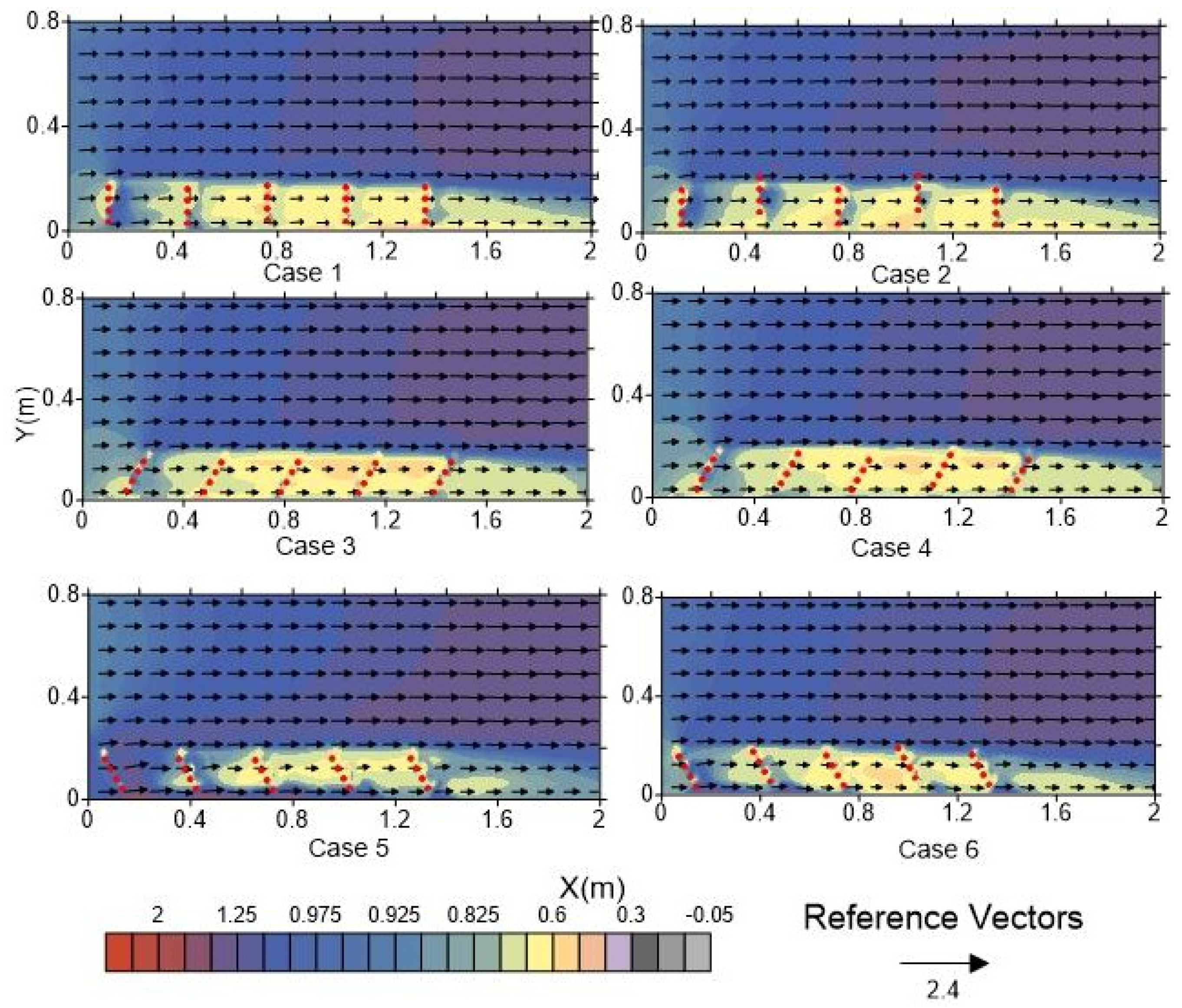
Figure 12 shows the distribution of the calculated dimensionless spatial velocity $\left(\frac{\underset{\_}{u}}{U},\frac{\underset{\_}{v}}{U}\right)$ at a flow depth of Z = 0.01 m. This figure reveals that the variation in the dimensionless spatial velocity $\left(\frac{\underset{\_}{u}}{U}\right)$ vector ranges from −0.05 to 2.2 within the considered zone of the flume. The average magnitude of the dimensionless spatial velocity within the main channel was 1.10, and that near the spur dike zone area was 0.77. Inside the main channel, the maximum velocity was obtained in case 2 (1.51), and the minimum was in case 4 (0.82) at Z = 0.02 m. Inside the spur dike zone, the spatial velocity was almost 6.5% lower for the staggered grid installation than for other installations.

Table 6. Increment of the spatial velocity in the main channel due to spur dike installation.

Unit	Case 1	Case 2	Case 3	Case 4	Case 5	Case 6
Percentage (%)	27.60	32.83	33.71	34.48	24.69	29.97

shows the velocity increment (in percentage) in the main channel due to the installation of different types of spur dikes. The average spatial velocity in the main channel was higher for the staggered installation because the tips of the second and third spurs of the dike in the staggered case were 0.05 m higher than those of the squared-type installation. Therefore, these spurs acted as one system and deflected more flow towards the main channel.

4.4. Flow Depth

Figure 13 shows the variation in the dimensionless water depth (d/h) (interpolated) around the spur dikes in the considered areas of the flume. In all cases, the depth of flow increases just upstream of the spur dike compared to that immediately downstream of the spur dike. At the tip of the spur dike, the experimental results varied more than the simulated results because of challenges in measuring the rapid and sharp variations in water depth. However, the maximum dam-up conditions were found in case 3 (experiment: 1.37; simulation: 1.12). The squared and staggered arrangements showed no significant difference (the difference in d/h between the staggered and squared installations was 0.06 for the experimental results and 0.22 for the simulated results).

4.5. Bed Shear Stress

Here, the bed shear stress was calculated from the Reynolds stress, as reported previously [21]. The longitudinal component was calculated using ${\tau }_b^x=-{\left(\rho \underset{\_}{\acute{w}\acute{u}}+\rho \underset{\_}{\acute{v}\acute{u}}\right)}_{bed}$, and the transverse component was calculated using ${\tau }_b^y=-{\left(\rho \underset{\_}{\acute{w}\acute{v}}+\rho \underset{\_}{\acute{u}\acute{v}}\right)}_{bed}$ and the bed shear stress ${\tau }_b=\sqrt{\left({\left({\tau }_b^x\right)}^2+{\left({\tau }_b^y\right)}^2\right)}$; dividing the bed shear stress by the approach flow bed shear stress yields the dimensionless parameter ${\tau }_b^{*}$. The distribution of the dimensionless bed shear stress is shown in Figure 14. Within the entire zone, the dimensionless bed shear varies from 0.02 to 2.2. For case 1, the tip of the first two spur dikes have maximum bed shears of 1.17 (X = 0.16 m, Y = 0.154 m) and 1.37 (X = 0.46 m, Y = 0.54 m). For case 2, at the same locations, the corresponding bed shear stresses were 0.95 and 0.82. However, in case 2, the maximum shear stress was 1.06 near the attachment area of the bank and third spur dike (X = 0.76 m, Y = 0.03 m). In case 3, the maximum dimensionless bed shear stress (1.56) was found at the tip of the first spur dike (X = 0.26 m, Y = 0.18 m). In case 4, the location of the maximum shear was the same as that in case 3, but the value was 7% higher. In case 5, an intense shear stress zone was observed near the first spur dike, where the maximum value reached 2.09. Similar shear stress patterns were observed in case 6, but the maximum value was 1.57, almost 24% lower than that in case 5.

Through laboratory experiments and numerical simulation, this study investigated the flow structure around slit-type permeable spur dike fields, including several layout alternatives for practical use. The previous discussion revealed that by using a slit-type permeable spur dike according to case 4, the approach velocity of flow can be reduced by a considerable amount within the spur dike zone.

4.6. Application of Slit-Type Spurs in the Brahmaputra–Jamuna River

The laboratory model was upscaled according to the Brahmaputra–Jamuna River channel width/depth ratio and installed in the numerical model with the Brahmaputra–Jamuna bathymetry and flow conditions recorded during the flood of 2011 (location is shown in Figure 1). During the flood of 2011 on the day of peak discharge (25 July 2011), the channel experienced a discharge of 27,395 m³/s, which was used as one of the boundary conditions of the model. The river sediment size, d_50, varied from 150 to 300 $\mu m$_, corresponding to a critical sediment velocity of nearly 0.4 to 0.5 m/s [61]. The total reach length was almost 3290 m long and almost 850 m wide, with bathymetry varying from −0.13 to 9.7 m PDW (meter Public Works Datum, corresponds 0.46 m below mean sea level. The performance of the slit-type spur was compared with that for no spur and conventional impermeable spur dikes. Five spurs aligned 120° with the flow were installed with a permeability of 71%, thereby maintaining similarity with the laboratory experiment. Each spur dike consisted of fifteen individual unsubmerged piles. The pile diameter was 1.25 m, and the gap between the piles was 6.25 m. The spacing of the spurs was 187.46 m, and the length was 113.75 m. In the impermeable case, a similar thickness of the spur was chosen with the same length and spacing.

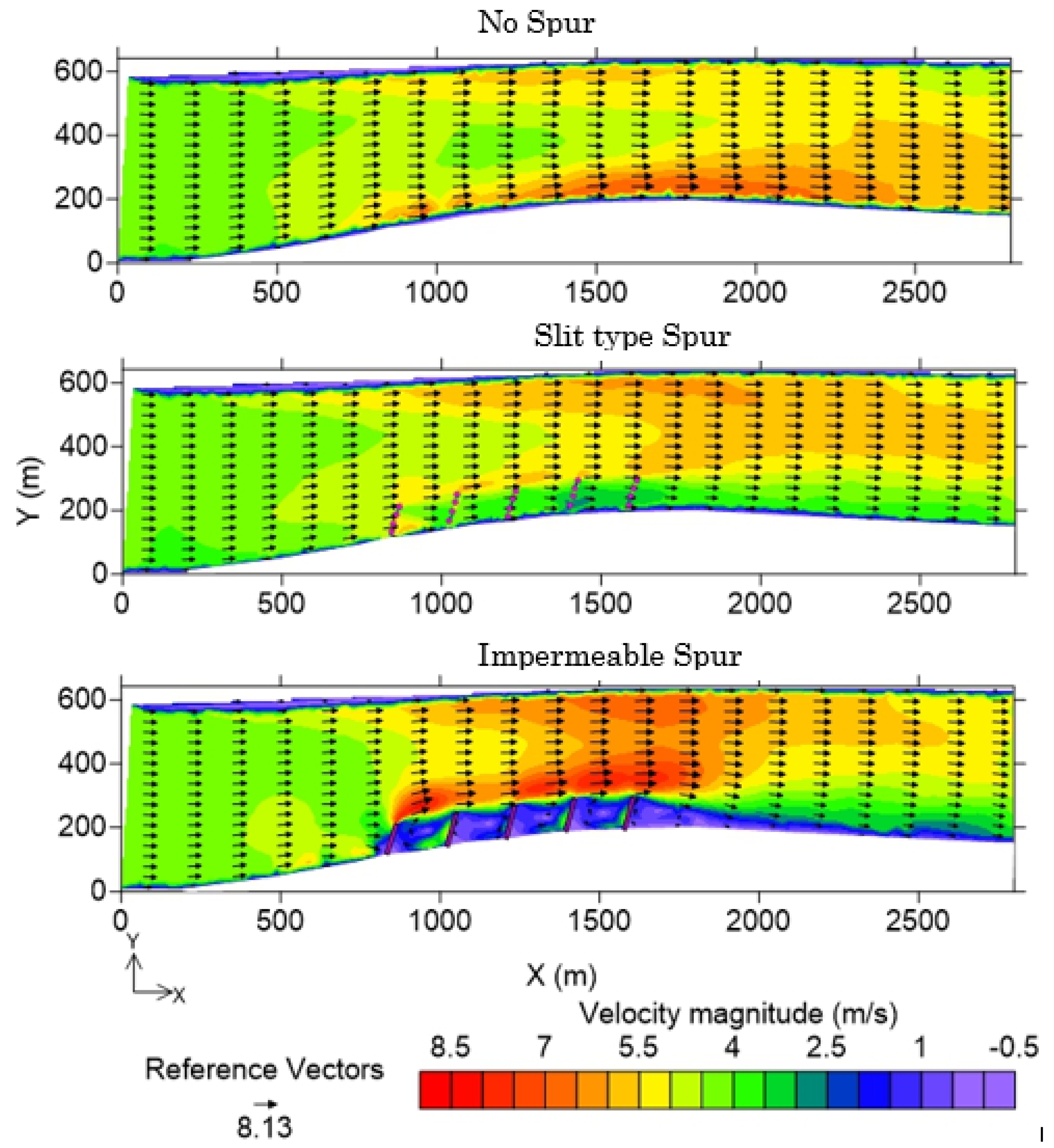
The distribution of the spatial velocity ($\underset{\_}{u}, \underset{\_}{v}$) for different conditions at Z = 14 m is shown in Figure 15 for the river. Without any structure, very high spatial velocities were observed near the right bank (from X = 1000 m~2100 m), ranging from 5.7 m/s to 6.9 m/s with an average velocity of 4.61 m/s. With the placement of slit-type spur dikes, the near-bank velocity decreased to 3.5 m/s (on average). It should be noted that when the flow entered the first embayment (between the first and second spurs, from X = 846 m to X = 1018 m), a relatively high velocity was observed (5.7 m/s) due to the bed topography and structure type. However, as the flow entered the succeeding embayment, the velocity gradually decreased, and when the flow left the spur dike region, the magnitude of the spatial velocity was 3.19 m/s. As confirmed in previous reports [8,17,28], a higher velocity at the tips of the spurs was also observed, which ranged from 5.3 to 5.76 m/s. Inside the main channel, the average velocity increased by almost 9.3% compared to that in the no spur case.

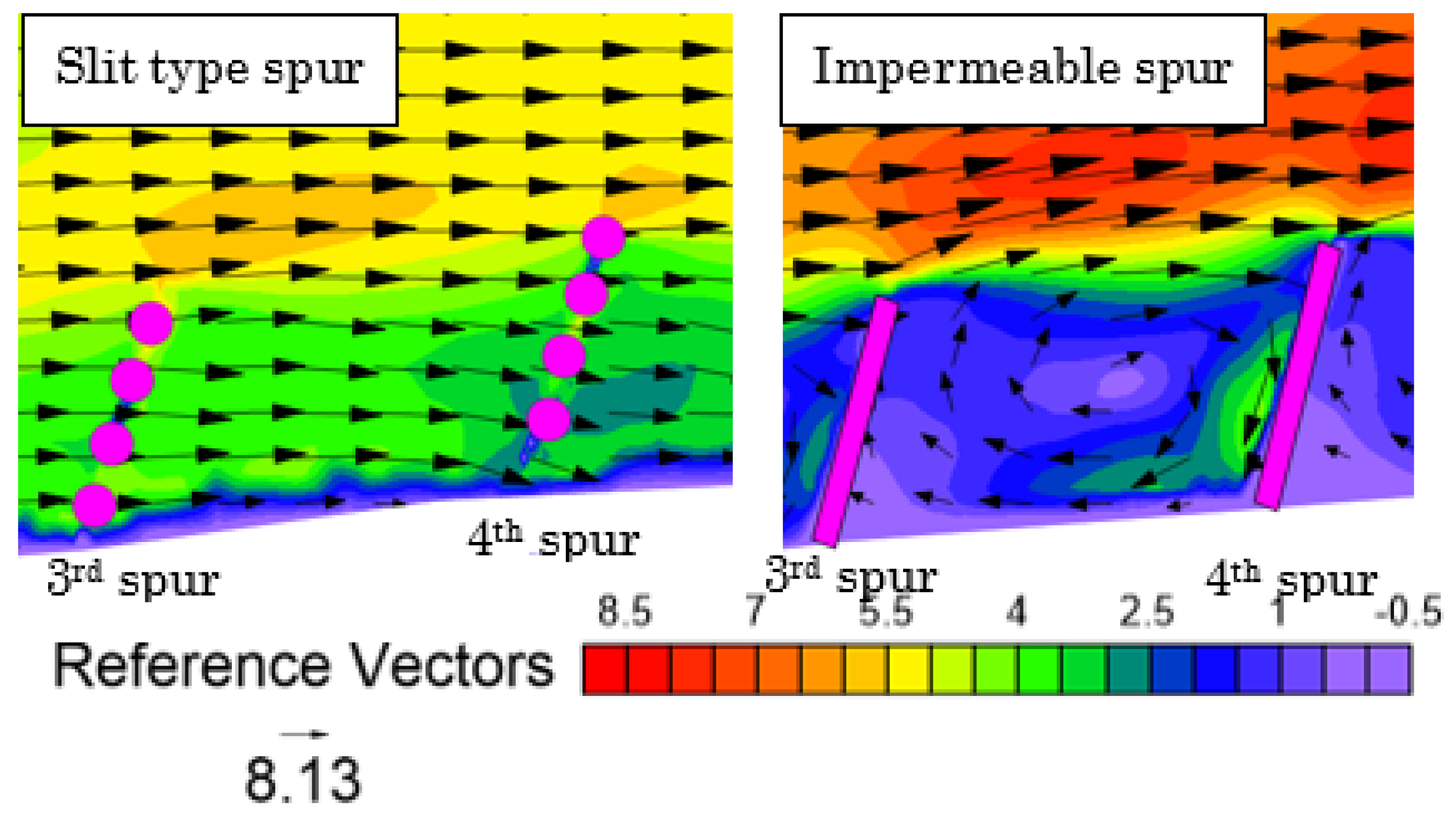
Due to the placement of the impermeable spurs, the average spatial velocity magnitude near the right bank (within the spur region) reached 1.38 m/s. Within the embayment, the strong recirculation of flow was observed. However, inside the embayment region, a concentrated flow velocity was observed in the downstream area. As an example, the spatial flow distribution in the third embayment is shown in Figure 16. At the downstream part of the embayment (adjacent to the 4th spur), the flow velocity reaches 3.9 m/s, and in the other areas, it varies between 0.16 m/s and 1.91 m/s. Such flow intensification was not observed in slit-type spur dike cases. Along the tips of the spurs, a very high velocity was observed, which ranged from 8.14 m/s to 7.44 m/s. Inside the main channel, the average velocity increased by almost 32% (average velocity was 6.06 m/s).

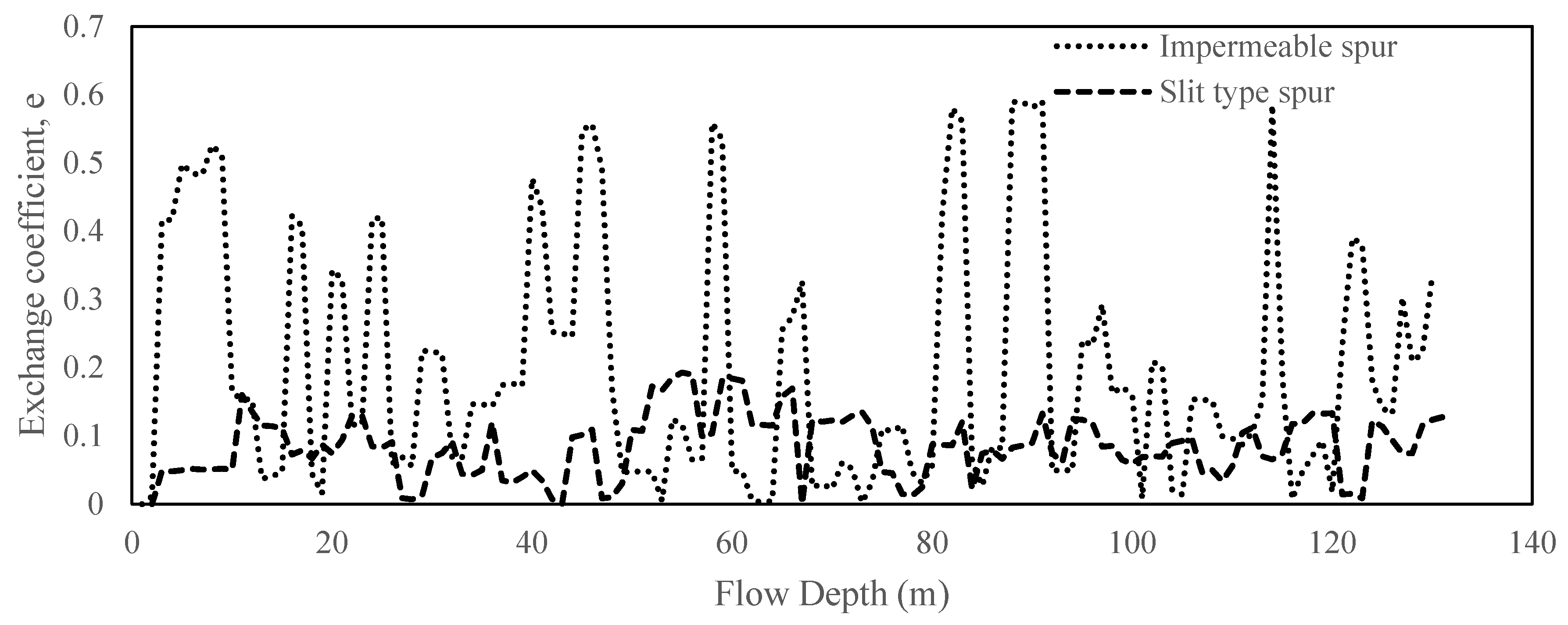
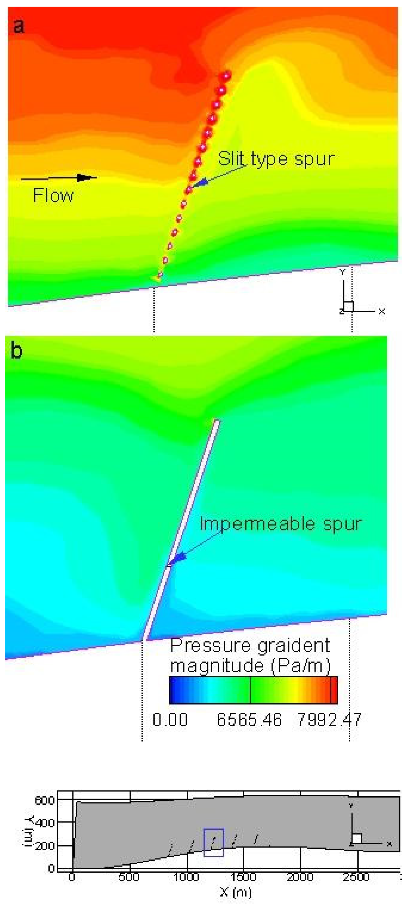
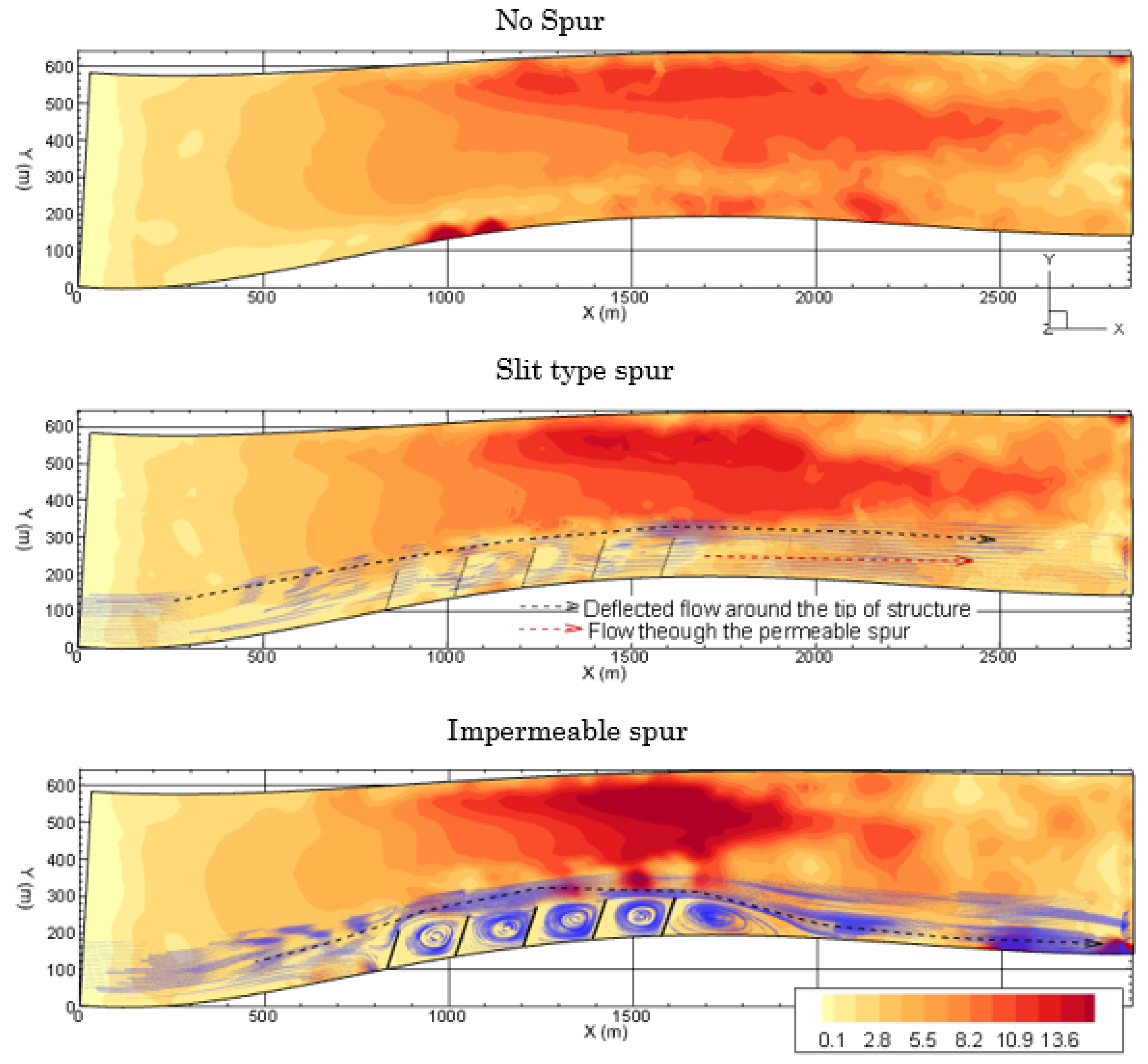
The distribution of the transverse velocity ($\underset{\_}{v},\underset{\_}{w}$) after the third spur is shown in Figure 17. Without any spur (case 1), the transverse velocity $\left(\underset{\_}{v}\right)$ varies from −0.52 m/s to 1.06 m/s. Near the bank, a high bank-directed velocity was observed (0.86 m/s). By placing slit-type or impermeable spurs, the transverse velocity can be lowered. In the slit-type spur case, at the same location, the transverse velocity component, $\underset{\_}{v}$, becomes 0.61 m/s, and in the impermeable spur case, it becomes −1.71 m/s. Such a strong recirculating velocity was also observed [4] in the real field. Researchers [62] also concluded that in the dead zones of impermeable spur-like structures, the main transport mechanism is transverse turbulent diffusion which controls the exchange processes with the mainstream. Therefore, this type of recirculating velocity can initiate or increase local scouring. Just after crossing the spur dike region, a high peak in the transversal velocity was observed in both cases, which resembled a DSL. Figure 18 shows the vortical structure of the mean flow using the Q criterion. This figure also indicates a 50% to 70% higher velocity in the DSL layer in the impermeable case than in other cases, especially at the tip of the first spur. The exchange coefficient between the third embayment and the main channel was calculated using the methods described in a previous study [63]. Figure 19 shows the distribution of the exchange coefficient e, inside the third embayment of impermeable and slit type spur with respect to flow depth. The average exchange coefficient, e, in this zone was 0.2 in case of impermeable spur, while it was 0.08 in case of slit type one, indicates weaker turbulence coherent structure in silt type spur. By performing large eddy simulation (LES) in case of river bank lateral cavities, it was concluded [64] that in transverse direction, pressure gradient contributes largely to flushing momentum out of the cavities (embayment in this case) while Reynolds normal stress and convection are responsible for its entraining into the cavity. Figure 20 shows a similar agreement of the higher-pressure gradient in case of slit type spur.

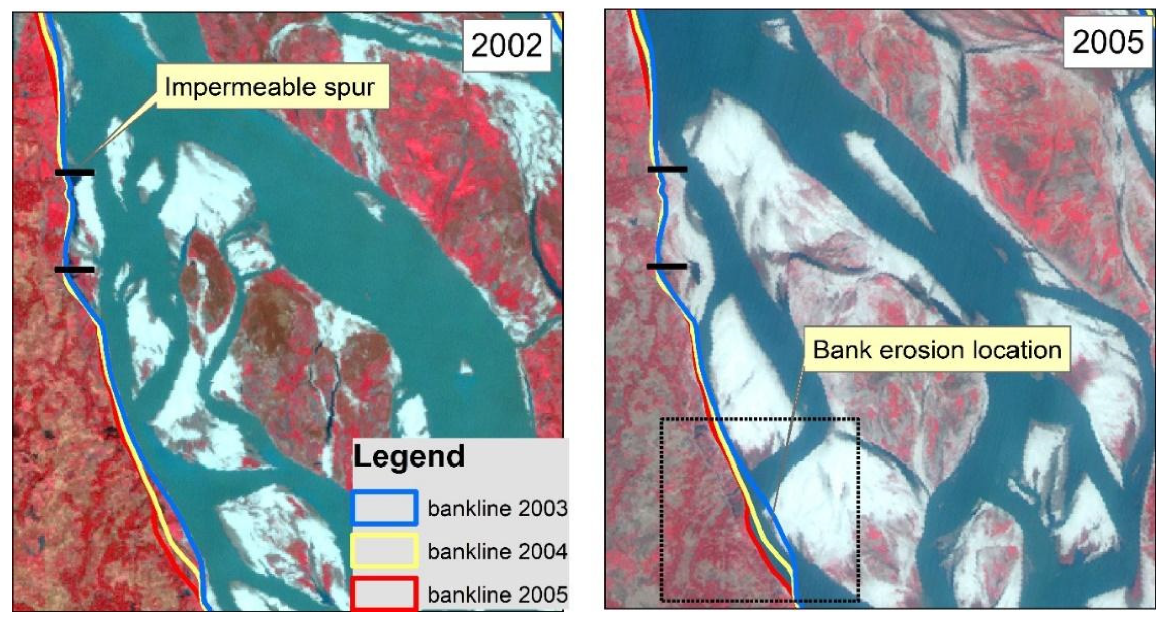
The distribution of bed shear stresses considering different conditions is shown in Figure 21. This figure indicates that in the no spur case, near the right bank, a high bed shear stress (8.2 to 14 N/m²) occurred, and due to the installation of the spur dike, this stress decreased. In the case of slit-type spurs, the shear stress varies from 1.45 N/m² to 4.15 N/m². Moreover, in the case of the impermeable spurs, the near-bank shear stress varies between 0.05 and 1.45 N/m², but in this case, the opposite bank experiences a higher (22%) bed shear stress compared to that for slit-type spurs. As the considered river is braided in nature, this increased bed shear stress may expedite the development of the channel. Another observation is that, due to the channel bathymetry in the impermeable spur case, the main deflected flow impacts the bank further downstream (at approximately X = 2500 m). However, in the case of the slit-type spur, the modified field prevents such a bank-directed flow. In a real field, such a phenomenon was also observed. Figure 22 shows such an example in the study river (at Dhunot, Bogra, Bangladesh). Two impermeable spurs were installed during 2002 (left side figure), and they worked well in subsequent years, but the deflected flow (as well as the sedimentation pattern) caused approximately 650 m of bank erosion approximately 6 km downstream from 2003 to 2005.

5. Conclusions

Through laboratory experiments and numerical simulations, this study investigated the flow structure around slit-type permeable spur dike fields, including several layout alternatives for practical use. The three-dimensional RANS equations were coupled with the k-ω SST turbulence model and the VOF method to capture the free water surface, and we found the hydrodynamic model results to be consistent with the experimental results for the flow structure around permeable pile spur dike fields and slit-type spur dike fields. This study revealed that by using a slit-type permeable spur dike, the approach velocity of flow can be reduced by a considerable amount within the spur dike zone. This type of spur dike is well suited for reducing the longitudinal velocity within the spur dike region. However, deflecting spurs were more successful at producing transverse flow to the opposite bank. This study also indicated that arranging the piles in a staggered grid in different spurs leads to better dike functionality in terms of reducing the bed shear stress and creating a quasi-uniform turbulence zone. However, high bed shear stress at the spur tip, especially for the initial spur, cannot be avoided in this type of spur dike field. Hence, for field applications of this type of structure, better protection measures should be taken for initial spurs.

From the field numerical simulation, it can be concluded that using slit-type spurs in a staggered pile position provides the best solution, as the velocity near the bank can be reduced by a considerable amount compared to that obtained with conventional impermeable spurs in a braided channel. Although the study is conducted in a small river reach of a braided river, it can be replicated in other alluvial rivers with fine sediment. The impermeable spur dike field creates a relatively strong transverse velocity (greater than the sediment suspension velocity) in the recirculation zone, which may aggravate local scouring. However, the recirculation velocity is weaker for slit-type spurs than for other structures. As the spatial velocity is gradually reduced in the slit-type spur zone, attention should be given to field installation methods, e.g., this approach may not work well if installed very near an eroding bank. Inside the first embayment, a relatively high velocity is observed. The bed shear stress can be effectively reduced using both slit and impermeable spurs, but in the case of impermeable spurs, the deflected flow can be intensified near the bank further downstream due to riverbed variations. This type of intensification can be avoided by using a slit-type permeable spur.

References

- Mutton, D.; Haque, C.E. Human Vulnerability, Dislocation and Resettlement: Adaptation Processes of River-bank Erosion-induced Displacees in Bangladesh. Disasters 2004, 28, 41–62. [Google Scholar] [CrossRef] [PubMed]
- Bryant, S.; Mosselman, E. Taming the Jamuna: Effects of river training in Bangladesh. In NCR Days 2017, Book of Abstracts; Hoitink, A.J.F., De Ruijsscher, T.V., Geertsema, T.J., Makaske, B., Wallinga, J., Candel, J.H.J., Poelman, J., Eds.; NCR publication: Atlanta, GA, USA, 2017; p. 114. [Google Scholar]
- Piégay, H.; Grant, G.; Nakamura, F.; Trustrum, N. Braided river management: From assessment of river behaviour to improved sustainable development. Braided Rivers 2006, 36, 257–275. [Google Scholar]
- Nakagawa, H.; Zhang, H.; Baba, Y.; Kawaike, K.; Teraguchi, H. Hydraulic characteristics of typical bank-protection works along the Brahmaputra/Jamuna River, Bangladesh. J. Flood Risk Manag. 2013, 6, 345–359. [Google Scholar] [CrossRef]
- Best, J.L.; Ashworth, P.J.; Sarker, M.H.; Roden, J.E. The Brahmaputra-Jamuna River, Bangladesh. In Large Rivers: Geomorphology and Management; Gupta, A., Ed.; John Wiley & Sons.: Hoboken, NJ, USA, 2007; pp. 395–430. [Google Scholar]
- Sarker, M.H.; Akter, J.; Ruknul, M. River bank protection measures in the Brahmaputra-Jamuna River: Bangladesh experience. In Proceedings of the International Seminar on’River, Society and Sustainable Development, Assam, India, 26–29 May 2011. [Google Scholar]
- Bhuiyan, A.F.; Hossain, M.M.; Heyl, R. Bank erosion and protection on the Brahmaputra (Jamuna) River. In Hydraulic Information Management; Brebbia, C.A., Blain, W.R., Eds.; WIT Press: Southampton, UK, 2002; p. 10. ISBN 1853129127. [Google Scholar]
- Koken, M.; Constantinescu, G. An investigation of the flow and scour mechanisms around isolated spur dikes in a shallow open channel: Conditions corresponding to the initiation of the erosion and deposition process. Water Resour. Res. 2008, 44, 1–19. [Google Scholar] [CrossRef]
- Rajaratnam, N.; Nwachukwu, B.A. Flow Near Groin-Like Structures. J. Hydraul. Eng. 1983, 109, 463–480. [Google Scholar] [CrossRef]
- Uijttewaal, W.S. Effects of Groyne Layout on the Flow in Groyne Fields: Laboratory Experiments. J. Hydraul. Eng. 2005, 131, 782–791. [Google Scholar] [CrossRef]
- Uijttewaal, W.S.J. The flow in groyne fields: Patterns and exchange processes. In Water Quality Hazards and Dispersion of Pollutants; Czernuszenko, W., Rowinski, P., Eds.; Springer: Boston, MA, USA, 2005; pp. 231–246. ISBN 0387233210. [Google Scholar]
- Li, Y.; Altinakar, M. Effects of a Permeable Hydraulic Flashboard Spur Dike on Scour and Deposition Yujian. In Proceedings of the World Environmental and Water Resources Congress 2016, West Palm Beach, FL, USA, 22–26 May 2016; pp. 399–409. [Google Scholar]
- Wu, B.; Wang, G.; Ma, J.; Zhang, R. Case Study: River Training and Its Effects on Fluvial Processes in the Lower Yellow River, China. J. Hydraul. Eng. 2005, 131, 85–96. [Google Scholar] [CrossRef]
- Ali, M.S.; Hasan, M.M.; Haque, M. Two-Dimensional Simulation of Flows in an Open Channel with Groin-Like Structures by iRIC Nays2DH. Math. Probl. Eng. 2017, 2017. [Google Scholar] [CrossRef]
- Cao, X.; Gu, Z.; Tang, H. Study on spacing threshold of nonsubmerged spur dikes with alternate layout. J. Appl. Math. 2013, 2013. [Google Scholar] [CrossRef]
- Gisonni, C.; Hager, W.H. Spur Failure in River Engineering. J. Hydraul. Eng. 2008, 134, 135–145. [Google Scholar] [CrossRef]
- Gu, Z.; Akahori, R.; Ikeda, S. Study on the transport of suspended sediment in an open channel flow with permeable spur dikes. Int. J. Sediment Res. 2011, 26, 96–111. [Google Scholar] [CrossRef]
- Kang, J.; Yeo, H.; Kim, S.; Ji, U. Permeability effects of single groin on flow characteristics. J. Hydraul. Res. 2011, 49, 728–735. [Google Scholar] [CrossRef]
- Duan, J.G. Three-dimensional Mean Flow and Turbulence around a Spur Dike. J. Hydraul. Eng. 2009, 135, 803–811. [Google Scholar] [CrossRef]
- Copeland, R.R. Bank Protection Techniques Using Spur Dikes; PN: Cebu, Philippines, 1983. [Google Scholar]
- Ghodsian, M.; Vaghefi, M. Experimental study on scour and flow field in a scour hole around a T-shape spur dike in a 90° bend. Int. J. Sediment Res. 2009, 24, 145–158. [Google Scholar] [CrossRef]
- Kuhnle, R.; Alonso, C. Flow near a model spur dike with a fixed scoured bed. Int. J. Sediment Res. 2013, 28, 349–357. [Google Scholar] [CrossRef]
- Kuhnle, R.A.; Alonso, C.V.; Shields, F.D. Local Scour Associated with Angled Spur Dikes. J. Hydraul. Eng. 2002, 128, 1087–1093. [Google Scholar] [CrossRef] [Green Version]
- Raudkivi, A.J. Permeable Pile Groins. J. Waterw. Port Coastal Ocean Eng. 1996, 122, 267–272. [Google Scholar] [CrossRef]
- Bakker, W.T.; Hulsbergen, C.H.; Roelse, P.; De Smit, C.; Svasek, J.N. Permeable groynes: Experiments and practice in the Netherlands. Coast. Eng. 1984, 1985, 649–660. [Google Scholar] [CrossRef]
- Koken, M.; Constantinescu, G. Flow and turbulence structure around a spur dike in a channel with a large scour hole. Water Resour. Res. 2011, 47, 1–19. [Google Scholar] [CrossRef]
- Mansoori, A.R. Study on Flow and Sediment Transport around Series of Spur Dikes with Different Head Shape. Bachelor’s Thesis, Kyoto University, Kyoto, Japan, 2014. [Google Scholar]
- Zang, H.; Nakagawa, H.; Kawaike, K.; Baba, Y. Experiment and simulation of turbulent flow in local scour around a spur dyke. Int. J. Sediment Res. 2009, 24, 33–45. [Google Scholar] [CrossRef]
- Alauddin, M. Morphological Stabilization of Lowland Rivers by Using a Series of Groynes. Ph.D. Thesis, Department of Civil Engineering, Nagoya University, Nagoya, Japan, 2011. [Google Scholar]
- Shampa; Hasegawa, Y.; Nakagawa, H.; Takebayashi, H.; Kawaike, K. Installation Effects on Three-Dimensional Flow Characteristics in a Slit-Type Permeable Spur Dike Field. In Proceedings of the 37th Annual Meeting of the Natural Disaster Society of Japan, Sendai, Japan, 6–7 October 2017; pp. 3–4. [Google Scholar]
- Zhang, H.; Nakagawa, H.; Kawaike, K.; Nishio, K. Experiment on Suspended sediment Transport around Bank Protection Structures. In Proceedings of the 5th International Conference on Water & Flood Management (ICWFM-2015), Dhaka, Bangladesh, 6–8 March 2015; pp. 127–134. [Google Scholar]
- Ettema, R.; Kirkil, G.; Muste, M. Similitude of Large-Scale Turbulence in Experiments on Local Scour at Cylinders. J. Hydraul. Eng. 2006, 132, 33–40. [Google Scholar] [CrossRef]
- Ettema, R.; Muste, M. Scale effects in flume experiments on flow around a spur dike in flatbed channel. J. Hydraul. Eng. 2004, 130, 635–646. [Google Scholar] [CrossRef]
- Safarzadeh, A.; Ali, S.; Salehi, A.; Zarrati, A.R. Experimental Investigation on 3D Turbulent Flow around Straight and T-Shaped Groynes in a Flat Bed Channel. J. Hydraul. Eng. 2016, 142, 1–15. [Google Scholar] [CrossRef]
- Dey, S.; Barbhuiya, A.K. Turbulent flow field in a scour hole at a semicircular abutment. Can. J. Civ. Eng. 2005, 32, 213–232. [Google Scholar] [CrossRef]
- Li, H.; Barkdoll, B.D.; Kuhnle, R.; Alonso, C. Parallel Walls as an Abutment Scour Countermeasure. J. Hydraul. Eng. 2006, 132, 510–520. [Google Scholar] [CrossRef]
- Klingemann, P.C.; Kehe, S.M.; Owusu, Y.A. Streambank Erosion Protection and Channel Scour Manipulation Using Rockfill Dikes and Gabions; Water Resources Research Institute, Oregon State University: Corvallis, OR, USA, 1984; pp. 1–872. [Google Scholar]
- Trampenau, T.; Goricke, F.; Raudkivi, A.J. Permeable Pile Groins. In Coastal Engineering; ASCE: Reston, VA, USA, 1996; Volume 122, pp. 2142–2151. [Google Scholar]
- Fukuoka, S.; Watanbe, A.; Kawaguchi, H.; Yasutake, Y. A study of permeable groins in series installed in a straight channel. Annu. J. Hydraul. Eng. 2000, 44, 1047–1052. [Google Scholar] [CrossRef]
- Li, Z.; Kohji, M.; Maeno, S.; Ushita, T.; Fujii, A. Hydraulic characteristics of a group of permeable groins constructed in an open channel flow. J. Appl. Mech. JSCE 2005, 8, 773–782. [Google Scholar] [CrossRef]
- Mioduszewski, T.; Maeno, S. Three Dimensional Around a Porous Analysis Spur of Flow Dike. J. Appl. Mech. 2005, 8, 793–801. [Google Scholar] [CrossRef]
- Menter, F.R. Two-equation eddy-viscosity turbulence models for engineering applications. AIAA J. 1994, 32, 1598–1605. [Google Scholar] [CrossRef] [Green Version]
- Hellsten, A. Some Improvements in Menter’s k-omega SST Turbulence Model. In Proceedings of the 29th AIAA Fluid Dynamics Conference 1998, Albuquerque, NM, USA, 15–18 June 1997; pp. 2–12. [Google Scholar]
- Menter, F.R.; Kuntz, M.; Langtry, R. Ten Years of Industrial Experience with the SST Turbulence Model, Proceedings of the Fourth International Symposium on Turbulence, Heat and Mass Transfer, Antalya, Turkey, 12–17 October 2003; Begell House: Antalya, Turkey, 2003; pp. 625–632. [Google Scholar]
- Hirt, C.W.; Nichols, B.D. Volume of fluid (VOF) method for the dynamics of free boundaries. J. Comput. Phys. 1981, 39, 201–225. [Google Scholar] [CrossRef]
- Zhou, L. Numerical Modelling of Scour in Steady Flows. Ph.D. Thesis, University of Lyon, Lyon, France, 2017. [Google Scholar]
- Weller, H.G. Derivation, modelling and solution of the conditionally averaged two-phase flow equations. Tech. Rep. 2002, TR/HGW 2, 9. [Google Scholar]
- Berberović, E.; Van Hinsberg, N.P.; Jakirlić, S.; Roisman, I.V.; Tropea, C. Drop impact onto a liquid layer of finite thickness: Dynamics of the cavity evolution. Phys. Rev. E Stat. Nonlinear Soft Matter Phys. 2009, 79, 036306. [Google Scholar] [CrossRef] [PubMed]
- Weller, H.G.; Tabor, G.; Jasak, H.; Fureby, C. A tensorial approach to computational continuum mechanics using object-oriented techniques. Comput. Phys. 1998, 12, 620–631. [Google Scholar] [CrossRef]
- OpenCFD Programmer’s Guide. Available online: http://foam.sourceforge.net/docs/Guides-a4/ProgrammersGuide.pdf (accessed on 26 March 2020).
- Next Foam Boundary Conditions- OpenFOAM-4.1. Available online: http://www.nextfoam.co.kr/lib/download.php?idx=135228&sid=235c1d3fc28364657dbb43ccfe025b25 (accessed on 27 March 2020).
- Roache, P.J. Quantification of Uncertainty in Computational Fluid Dynamics. Annu. Rev. Fluid Mech. 1997, 29, 123–160. [Google Scholar] [CrossRef] [Green Version]
- Roache, P.J. Perspective: Validation—What does it mean? J. Fluids Eng. Trans. ASME 2009, 131, 0345031–0345034. [Google Scholar] [CrossRef]
- Blocken, B.; Gualtieri, C. Ten iterative steps for model development and evaluation applied to Computational Fluid Dynamics for Environmental Fluid Mechanics. Environ. Model. Softw. 2012, 33, 1–22. [Google Scholar] [CrossRef]
- Santhi, C.; Arnold, J.G.; Williams, J.R.; Dugas, W.A.; Srinivasan, R.; Hauck, L.M. Validation of the SWAT model on a large river basin with point and nonpoint sources. J. Am. Water Resour. Assoc. 2002, 37, 1169–1188. [Google Scholar] [CrossRef]
- Bracmort, K.S.; Arabi, M.; Frankenberger, J.R.; Engel, B.A.; Arnold, J.G. Modeling Long-Term Water Quality Impact of Structural BMPs. Trans. Am. Soc. Agric. Biol. Eng. 2006, 49, 367–374. [Google Scholar] [CrossRef] [Green Version]
- Gupta, H.V.; Sorooshian, S.; Yapo, P.O. Status of Automatic Calibration for Hydrologic Models: Comparison With Multilevel Expert Calibration. J. Hydrol. Eng. 2001, 4, 135–143. [Google Scholar] [CrossRef]
- Melville, B.W.; Coleman, S.E. Bridge Scour; Water Resources Publication: Littleton, CO, USA, 2000; ISBN 1887201181. [Google Scholar]
- Zhang, H.; Nakagawa, H.; Ogura, M.; Mizutani, H. Experiment Study on Channel Bed Characteristics around Spur Dykes of Different Shapes. J. Jpn. Soc. Civ. Eng. Ser. B1 2013, 69, 489–499. [Google Scholar] [CrossRef] [Green Version]
- Dubief, Y.; Delcayre, F. On coherent-vortex identification in turbulence. J. Turbul. 2000, 1, 11. [Google Scholar] [CrossRef]
- Van Rijn, L.C. Principles of Sedimentation and Erosion Engineering in Rivers, Estuaries and Coastl Seas; Aqua Publications: Blokzijl, The Netherlands, 2005; pp. 1–15. [Google Scholar]
- Gualtieri, C. Numerical simulation of flow patterns and mass exchange processes in dead zones. In Proceedings of the 4th International Congress on Environmental Modelling and Software—Barcelona, Catalonia, Spain, 7–10 July 2008; Volume 1, pp. 150–161. [Google Scholar]
- Weitbrecht, V.; Socolofsky, S.A.; Jirka, G.H. Experiments on Mass Exchange between Groin Fields and Main Stream in Rivers Volker. J. Hydraul. Eng. 2007, 134, 173–183. [Google Scholar] [CrossRef]
- Ouro, P.; Juez, C.; Franca, M. Drivers for mass and momentum exchange between the main channel and river bank lateral cavities. Adv. Water Resour. 2020, 137, 103511. [Google Scholar] [CrossRef]
Figure 1.
Permeable spur dike in Bangladesh. The shaded area indicates the location perpendicular to the structure.(a) a failed semipermeable spur dike in the Brahmaputra–Jamuna River. (b) initial spur constructed. (c) reinforced cement concrete (RCC) part of the dike. (d) acoustic Doppler current profiler (ADCP).
Figure 2.
Conceptual description of the flow distribution around a spur dike.
Figure 3.
Experimental configuration (unit: m).
Figure 4.
Example of the computational mesh (case 1).
Figure 5.
Comparison of experimental and simulated surface velocities for case 1.
Figure 6.
Example comparison of experimental and simulated three-dimensional velocities and water depths.
Figure 7.
Dimensionless longitudinal velocity vector () 0.11 m from the right bank. The contour shows the variation of the longitudinal velocity component ( ).
Figure 8.
Box-and-whisker plot of the magnitude of the dimensionless longitudinal velocity .
Figure 9.
The ratio of the depth-averaged longitudinal velocity decrement to the approach velocity 0.02 m upstream and 0.02 m downstream of the spur dike.
Figure 10.
The dimensionless transverse velocity vector 0.02 m upstream of the third spur dike. The contour shows the variation in the transverse velocity component .
Figure 11.
Visualization of the vortex flow structure using the Q criterion for case 2.
Figure 12.
Dimensionless spatial velocity at Z = 0.01 m. The contour shows the variation in the longitudinal velocity component .
Figure 13.
Spatial distribution of the dimensionless water depth (d/h) in different cases.
Figure 14.
Dimensionless bed shear stress calculated from the Reynolds stress.
Figure 15.
The distribution of the spatial velocity () in m/s. The contours show the magnitude of the spatial velocity ( in m/s.
Figure 16.
The distribution of the spatial velocity () in m/s inside the third embayment. The contours show the magnitude of the spatial velocity ( in m/s.
Figure 17.
The distribution of the transverse velocity () in m/s. The contours show the variation in the transverse velocity in m/s.
Figure 18.
Visualization of the vortical structure of the mean flow using the Q criterion for slit-type and impermeable spurs. The magnitude of the velocity is shown in (m/s).
Figure 19.
The distribution of exchange coefficient inside the third embayment.
Figure 20.
Distribution of pressure gradient magnitude around the third spur (near bed): (a) slit type spur, (b) impermeable spur.
Figure 21.
The distribution of the bed shear stress along the spur zone (the blue line shows the stream trace).
Figure 22.
Bank erosion downstream of the impermeable spur at Brahmaputra–Jamuna (location: Dhunot, Bogra, Bangladesh).