Impact of Disdrometer Types on Rainfall Erosivity Estimation
by
 , , , and
Lisbeth Lolk Johannsen
1,* ,
,
Nives Zambon
1,
Peter Strauss
2,
Tomas Dostal
3,
Martin Neumann
3,
David Zumr
3 ,
,
Thomas A. Cochrane
4 and
Andreas Klik
1 1
Institute for Soil Physics and Rural Water Management, University of Natural Resources and Life Sciences, 1190 Vienna, Austria
2
Institute for Land and Water Management Research, 3252 Petzenkirchen, Austria
3
Faculty of Civil Engineering, Czech Technical University in Prague, 166 29 Prague 6, Czech Republic
4
Department of Civil and Natural Resources Engineering, University of Canterbury, Christchurch 8140, New Zealand
*
Author to whom correspondence should be addressed.
Water 2020, 12(4), 963; https://doi.org/10.3390/w12040963
Submission received: 25 February 2020
/
Revised: 25 March 2020
/
Accepted: 26 March 2020
/
Published: 28 March 2020
(This article belongs to the Section Hydrology)
Abstract
:Soil erosion by water is affected by the rainfall erosivity, which controls the initial detachment and mobilization of soil particles. Rainfall erosivity is expressed through the rainfall intensity (I) and the rainfall kinetic energy (KE). KE–I relationships are an important tool for rainfall erosivity estimation, when direct measurement of KE is not possible. However, the rainfall erosivity estimation varies depending on the chosen KE–I relationship, as the development of KE–I relationships is affected by the measurement method, geographical rainfall patterns and data handling. This study investigated how the development of KE–I relationships and rainfall erosivity estimation is affected by the use of different disdrometer types. Rainfall data were collected in 1-min intervals from six optical disdrometers at three measurement sites in Austria, one site in Czech Republic and one site in New Zealand. The disdrometers included two disdrometers of each of the following types: the PWS100 Present Weather Sensor from Campbell Scientific, the Laser Precipitation Monitor from Thies Clima and the first generation Parsivel from OTT Hydromet. The fit of KE–I relationships from the literature varied among disdrometers and sites. Drop size and velocity distributions and developed KE–I relationships were device-specific and showed similarities for disdrometers of the same type across measurement sites. This hindered direct comparison of results from different types of disdrometers, even when placed at the same site. Thus, to discern spatial differences in rainfall characteristics the same type of measurement instrument should be used.
1. Introduction
Soil erosion is recognized as a major threat to soil resources and the environment globally [1]. The initial detachment of soil particles through splash erosion, where soil particles are disaggregated and mobilized, is influenced by the rainfall erosivity. Erosivity is dependent on the rainfall characteristics, such as drop size and fall velocity, and the rainfall intensity (I). Thus, rainfall kinetic energy (KE) has been applied as a measure of potential soil loss [2]. Direct measurement of KE has been labor-intensive and costly, so as a means to calculate the kinetic energy of rainfall, when data of drop size and velocity are not available, KE–I relationships have been developed. The empirical relationships have been established from studies measuring the drop size and fall velocity at a specific site. The equations relate KE with rainfall intensity and make it possible to estimate KE only by knowing the intensity of the rainfall.
Several models of KE–I relationships including linear [3,4], exponential [5,6,7,8], logarithmic [9,10] and power law [11,12,13,14] have been found to fit the empirical data the best. The large variation in the KE–I relationships established in the literature is caused by the use of different measurement methods, limited sampling, errors introduced during interpretation of data and rainfall patterns [15]. Rainfall kinetic energy has been measured by methods such as the flour pellet technique [16], photographic method [17] and disdrometer measurements [5,7,8,18], all of which have their own limitations.
The KE–I relationships have been developed on data from various geographical and meteorological conditions, where site-specific rainfall patterns lead to differences in drop size and velocity distributions. Thus, many relationships are only valid under the conditions on which they were calibrated, resulting in a limited use outside of these areas [15,19,20]. To overcome this, van Dijk et al. [15] used several exponential relationships from around the world to make one universally predictive KE-I relationship based on an averaging of the empirical parameters (Table 1).
Other commonly used universal KE–I relationships are the Wischmeier and Smith [10] and Brown and Foster [16] equations as these have been used in erosivity estimations and to predict soil loss in the Universal Soil Loss Equation (USLE) and its revised version (RUSLE). A modified version of the Brown and Foster equation, as proposed by McGregor et al. [21], is now used in the updated RUSLE2 model (Table 1). The (R)USLE is the most widely used quantitative model for soil erosion risk assessment and includes several parameters, one of them being the rainfall erosivity. The rainfall erosivity is defined as the product of the total event KE and the 30-minute maximum rainfall intensity, as rainfall KE alone may not provide the best estimation of erosivity [10]. However, if KE is estimated by an equation based on rainfall intensity, then the whole calculation of KE and rainfall erosivity is actually based on rainfall intensity [22].
As rainfall intensity, unlike KE, is an extensively measured rainfall parameter, this makes KE–I relationships useful for spatial and temporal rainfall erosivity estimation. This has enabled the mapping of rainfall erosivity to show global and regional erosion risk areas [23,24,25,26] and projections of future rainfall erosivity due to altered rainfall patterns [27].
The extensive use of these KE–I relationships in soil erosion risk assessment demonstrates the importance of choosing the most suitable model, as erosivity estimates will vary according to the chosen KE–I relationship [19,28,29]. Angulo-Martínez et al. [19] stated that disdrometer data are therefore necessary to check which KE–I relationship works best for the specific site conditions.
Disdrometers are automated rainfall measurement instruments, which are able to continuously measure the number, size and velocity of falling raindrops and are thus able to give direct measurements of the kinetic energy. Disdrometer data are useful in a wide range of fields due to their high temporal resolution and has been used for the development of KE–I relationships at several sites worldwide [5,6,13,14,18,30,31,32,33]. However, despite the technological improvement, disdrometer data are still subject to measurement uncertainty. This uncertainty stems from both instrumental limitations (e.g., splashing, reduced measuring area, internal processing of drops) and environmental influences such as wind. Several studies have tried to quantify these measurement uncertainties and establish possible correction procedures [34,35,36,37,38]. Variations in rainfall measurements between disdrometers and between disdrometers and rain gauges have been observed [35,39,40,41]. In addition, disdrometers have been shown to measure different drop size distributions even when located at the same site [38,42,43]. The drop size distribution varies naturally in time and space, but disdrometers situated next to each other showed different distributions, which would not be explained by this natural variation [39]. Therefore, the development of a new KE–I relationship based on disdrometer data, is likely to be dependent not only on the geographical rainfall pattern, but also on the type of disdrometer. The measurement uncertainty of disdrometer data presents a need to assess the effect of different disdrometer types on the estimation of rainfall erosivity.
In this study, we aimed to (i) investigate the drop size and velocity distribution measured by three types of disdrometers, (ii) develop new KE–I relationships for five sites based on disdrometer data, (iii) compare the performance of KE–I relationships from the literature on these data, and (iv) validate the site-specific KE–I relationships on rain gauge data, in order to better assess the uncertainties in rainfall erosivity estimation.
2. Materials and Methods
2.1. Description of Sites and Devices
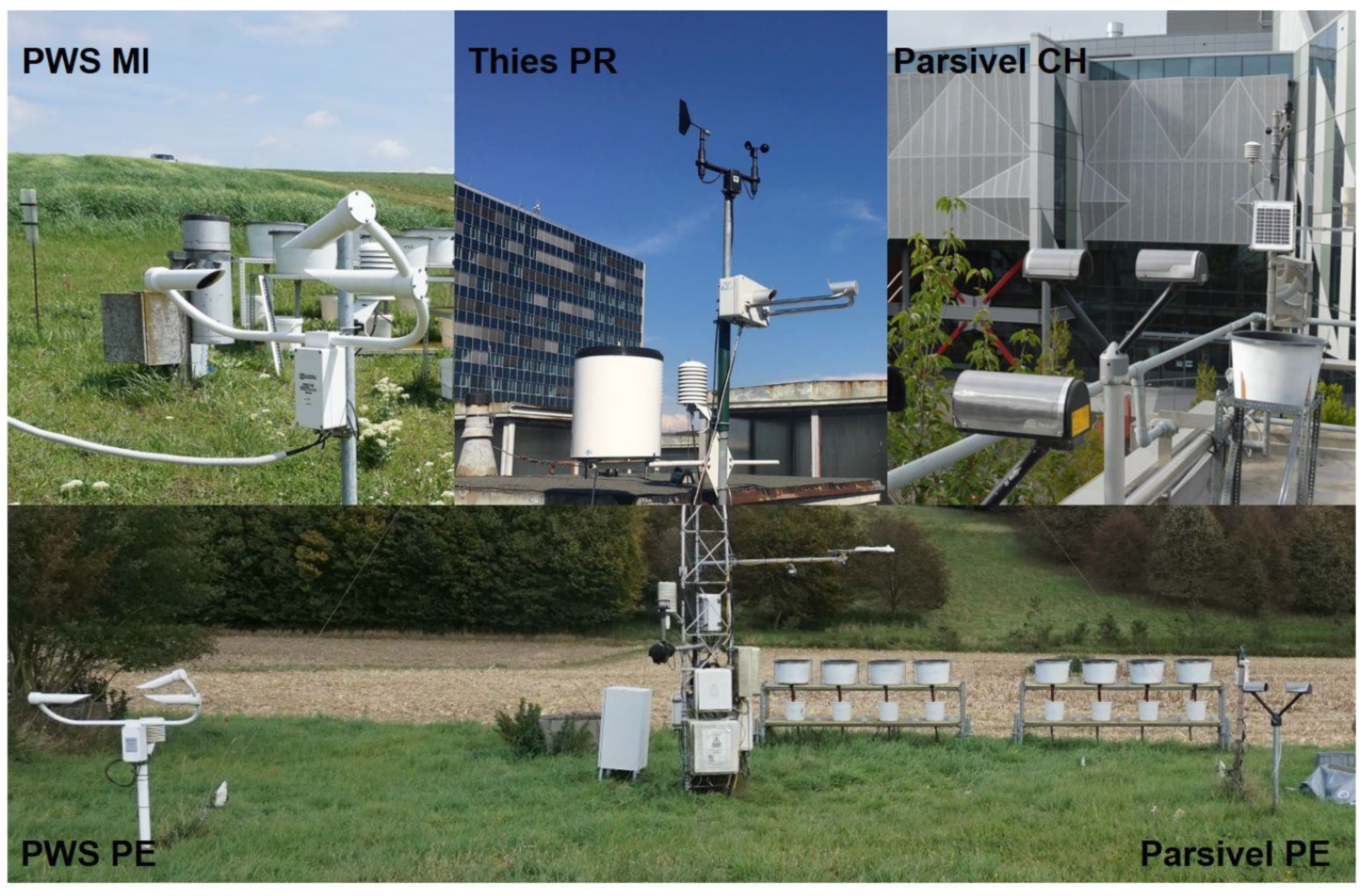
Measurement of rainfall was carried out at three sites in eastern Austria: Mistelbach (MI), Petzenkirchen (PE) and Rauchenwarth (RA), as well as one site in Prague (PR), Czech Republic and one site in Christchurch (CH), New Zealand. The measurement site locations and mean annual precipitation and temperature can be seen in Table 2 [44,45,46,47,48]. Figure 1 shows the set-up of the disdrometers at the measurement sites. Rainfall data were collected in 1-minute intervals using optical disdrometers with laser-based sensors, which measure precipitation by determining the size and velocity of raindrops when falling through the measuring area. The rainfall was measured in the period between 2014 to 2019, but with varying amounts of data for each site and disdrometer. The number of rainy minutes used for analysis for each site (after filtering) can be seen in Table 4.
The PWS100 Present Weather Sensor from Campbell Scientific (PWS100) was installed at the Mistelbach (PWS MI) and Petzenkirchen sites (PWS PE). The PWS100 has a measuring area of 40 cm2, measures in the intensity range of 0 to 400 mm h−1 and classifies precipitation into 34 drop size and 34 velocity classes of varying width.
The Laser Precipitation Monitor from Thies Clima (Thies) was installed at the sites in Rauchenwarth (Thies RA) and Prague (Thies PR). Each Thies disdrometer has a device-specific measuring area. For the Thies in Prague, the exact measuring area was 44.1 cm2. The device-specific measuring area for the Thies installed in Rauchenwarth was not known and thus the standard measuring area of 45.6 cm2 was used for this disdrometer. Thies measures intensities from less than 0.005 to 1000 mm h−1 and has 22 drop size classes and 20 velocity classes.
The first version of OTT Parsivel (Parsivel) from OTT Hydromet was installed in Petzenkirchen (Parsivel PE) and in Christchurch (Parsivel CH). It has a measuring area of 54 cm2 and measures intensities from 0.001 to 1200 mm h−1. Parsivel has 32 drop size and velocity classes, although the two smallest classes are not used as these drop sizes are outside the measurement range of the device.
2.2. Filtering of Data
The disdrometers are capable of discerning the type of precipitation into different classes according to the World Meteorological Organizations significant present and forecast weather code (WMO METAR/SPECI w’w’ Table 4678) [49]. Based on this classification, only the minutes with rainfall and drizzle or a mixture of the two were selected for further analysis. The Parsivel CH did not output this classification of the precipitation. Thus, data measured during the winter months, where snow could be present, were manually removed before further filtering.
Drops deviating more than 50% from the value of the Atlas et al. [50] diameter–terminal fall velocity relationship were not included in the calculation of KE for establishing the KE–I relationships. A similar filtering was also applied in other studies [38,51,52,53,54,55,56] to remove erroneously measured drops. Both Parsivel data sets were also cut off for rainfall intensities above 60 mm h−1 to eliminate outliers that were not removed by the filtering.
2.3. Development of Site-Specific Rainfall Kinetic Energy–Intensity Relationships
The kinetic energy was determined from the matrix of drop size and velocity classes given by each disdrometer. The rainfall kinetic energy per area per unit time, KE (J m−2 h−1), was calculated for each 1-min data retrieval as:
where Ni,j is the number of detected raindrops in size class i and velocity class j, A is the measuring area of the disdrometer (m2), Δt (1/60 h) is the interval of data collection, ρ is the density of water (g cm−3), Di is the mean drop diameter (mm) of size class i and vj is the mean fall velocity (m s−1) of velocity class j.
The rainfall amount, R (mm), and intensity, I (mm h−1), were calculated from the drop size distribution by
where A is the measuring area of the disdrometer (mm2).
For each site and disdrometer, an exponential KE–I relationship was established based on the calculated intensity and KE for each minute. The three-parameter exponential equation (Equation (4)), where a, b and c are empirical constants, has one more parameter than the commonly used linear, logarithmic or power law equations, but it has been recommended as a better fit to the KE–I relationship [17,57]. Linear, logarithmic and power law models suggest that there is no maximum limit to kinetic energy at increasing intensities. However, research has shown that an upper limit may exist [7]. This was also recognized by Wischmeier and Smith [10] as they adapted their equation to remain constant for intensities above 76 mm h−1.
The parameter a in the exponential model describes an upper limit to the kinetic energy content of rainfall, that is the maximum kinetic energy the rainfall can contain per mm. The exponential model also results in a lower limit of KE at very low intensities, although this may not necessarily be a real phenomenon of rainfall KE [15].
To obtain the best fitting exponential KE–I relationship for each site and disdrometer, the data were fitted with a nonlinear regression by nonlinear least squares [58]. The equation parameters were found by successive approximations to the three-parameter exponential model using the nonlinear least squares function (nls) within the statistical language R [59].
To compare the measured KE from each disdrometer and site to that calculated from the KE–I relationships in Table 1, the disdrometer intensities found from Equation 3 were used in the equations. The logarithmic equation (WS) yielded negative KE values at an intensity below 0.043 mm h−1. These negative values were not included in the summation of KE.
2.4. Validation of Site-Specific Rainfall Kinetic Energy–Intensity Relationships on Rain Gauge Data
The daily rainfall measured by the rain gauge at each site was compared to that measured by the disdrometers for days where both rainfall measurement devices measured more than 1 mm rainfall. A weighing principle rain gauge with a rainfall resolution of 0.01 mm was situated in PE. In MI and PR, the rain gauges were of the tipping bucket type with a rainfall resolution of 0.1 mm. The rain gauge in CH was also a tipping bucket with a rainfall resolution of 0.2 mm. Rain gauge data were not available for the Rauchenwarth site. The number of rainy days compared were 42, 45, 37, 26 and 65 for PWS MI, PWS PE, Thies PR, Parsivel PE and Parsivel CH, respectively.
For validation of the site-specific KE–I relationship established on the disdrometer data, the intensity measured by the rain gauges was used in the site-specific relationship to calculate KE. For the validation of rain gauge values (rain and KE), the unfiltered values from the disdrometers were used, as this would otherwise not correspond to the values measured by the rain gauges.
The percent bias (PBIAS), root mean squared error (RMSE) and the mean absolute error (MAE) were used to quantify the errors in KE estimation between disdrometers and literature KE–I relationships, and in rainfall measurements between disdrometers and rain gauges.
3. Results and Discussion
3.1. Drop Size and Velocity Distributions
The drop size and velocity distribution obtained by the devices were similar for disdrometers of the same type, despite being placed at different sites (Figure 2). PWS MI and PWS PE both measured the largest number of drops in the class with a mean diameter of 1.1 mm and mean velocity of 4.4 m s−1. They also both followed the terminal velocity line well and had few drops in classes deviating more than 50% from this line. Thies RA and Thies PR both registered the highest number of drops at a mean diameter of 0.3 mm and mean velocity of 1.2 m s−1. Both Thies disdrometers recorded a large number of small drops with high velocities, although it was more pronounced at the RA site. This was also observed by Angulo-Martínez et al. [19,38] and Wilken et al. [28], who speculated it may be due to splashing and break up of drops on the instrument, or a larger occurrence of edge events due to the smaller width of the laser beam. The two Parsivel disdrometers did not record the largest number of drops in the same class. Parsivel PE measured the most drops at a diameter of 0.8 mm and 4.4 m s−1, while Parsivel CH classified the most drops into the class with a diameter of 0.4 mm and a velocity of 2.6 m s−1. This may be due to the difference in rainfall regime. However, despite their spatial separation, both Parsivel disdrometers showed similar distributions with an overestimation of the velocity of the majority of drops (up to around a diameter of 1 mm) compared to the terminal velocity line. This distribution was also observed in other studies [41,43,60].
The difference in raindrop distribution between disdrometers arise from differences in the instrument design, measuring area, drop size and velocity classification and internal algorithms. This hinders the direct comparison of rainfall measurements between disdrometers. The device-specific distribution is seen from the comparison of PWS PE and Parsivel PE, which were situated at the same site, but presented different drop size and velocity distributions. This shows that the disdrometer type affects rainfall measurement to such a degree that it makes it difficult to determine the actual geographical rainfall characteristics of the measurement site.
According to the disdrometer manuals, all three disdrometer types have some inbuilt filtering processes, which correct for erroneously measured drops. The amount of information is limited for Thies and Parsivel, where only the effect of possible edge events is mentioned [61,62]. For PWS100 more detail is given e.g., about the so-called unknown drops. These are drops, that for example have been measured as travelling too fast for their size [63]. The unknown drops are removed from the matrix of drop sizes and velocities, which could be a reason for the small number of drops deviating from the terminal fall velocity line. The well-defined drop size and velocity distribution of the PWS100 may suggest that this disdrometer provides better rainfall measurement, especially with regard to kinetic energy.
3.2. Filtering of Drops
The filtering of drops deviating more than 50% from the terminal velocity line by Atlas et al. [50] resulted in a loss of drops. The number of drops filtered out varied between disdrometers and sites. As the PWS MI and PWS PE disdrometers generally follow the terminal velocity line very well, only 3.6% and 4.3% of all drops were removed for PWS MI and PWS PE, respectively. For Thies RA, the filtering excluded 53.6% drops, and for Thies PR it excluded 25.6% drops. Parsivel PE and Parsivel CH had 58.8% and 37.7% of the measured drops removed, respectively. The filtering of drops corresponded to a decrease in measured rainfall amounts of 0.4% for PWS MI and 2.0% for PWS PE. Even though Thies had up to half of the drops filtered out, the small size of the filtered drops resulted in a reduction in rainfall of 12.1% for Thies RA and 5.3% for Thies PR. The Parsivel disdrometers had the highest decrease in measured rainfall due to filtering with 27.3% and 20.3% for Parsivel PE and Parsivel CH, respectively.
Filtering of disdrometer data based on the drop size and velocity deviating from the terminal velocity line has been applied in several other studies [38,53,54,55,56]. The percentage of removed drops ranged from 12% to 24% in these studies. On the data measured by a Parsivel disdrometer, Jaffrain and Berne [52] employed a filter of 60% of the terminal drop velocity model, which lead to 25% of drops being removed. This corresponded to 3.5% of the total rainfall recorded.
The effect of filtering on the mean drop size and velocity can be seen in Table 3. For PWS MI and PWS PE, there was no difference before and after filtering. For Thies and Parsivel, there was a slight increase in mean drop size as all the small, but fast drops had been filtered out. For Thies PR and Parsivel PE the mean velocity increased.
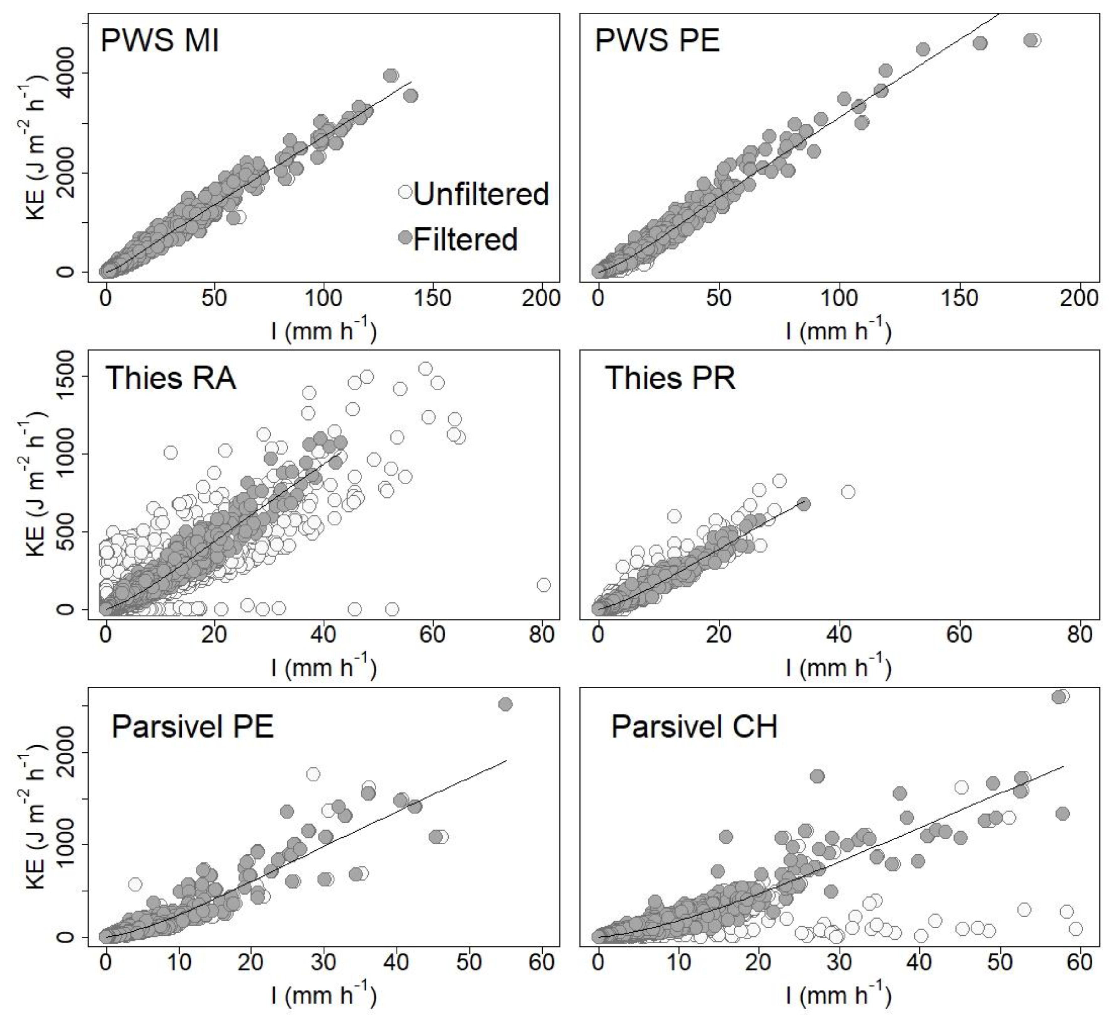
The reason for filtering the raindrops is to remove erroneously measured drops, which could potentially affect the estimation of rainfall characteristics measured by the disdrometer, such as KE. The spurious drops can occur due to multiple drops falling at one time, splashing from the instrument or wind effects [51,52]. However, filtering could remove some real raindrops, but in order to reduce the number of outliers, a filtering can be necessary. This was especially the case for the Thies and Parsivel data, as seen in Figure 3, where the scattered nature of the KE–I relationship for each disdrometer before filtering is shown. Thies RA and Parsivel CH especially showed a high degree of scatter. Points of high intensity but low KE were present in these plots, which could indicate the presence of snow. Wind may also have affected the degree of scatter of the KE–I points, as the velocity distribution has been found to broaden under windy conditions due to sub- and super-terminal drops [64]. Johannsen et al. [43] observed the importance of the installation of a wind protection shield for the Thies, as the drop velocity of small drops was seen to increase for events without the wind protection shield installed.
3.3. Development of New Rainfall Kinetic Energy–Intensity Relationships
The filtering of the data generally removed outliers and led to less scatter of the plotted KE and I, although for the Parsivel disdrometers some scatter still persists (Figure 3). For PWS MI, PWS PE and Thies PR filtering did not affect the fitting of the KE–I relationships greatly. However, the scattered nature of the data from Thies RA and Parsivel CH made filtering necessary to get a good fit of the model. The filtering of the disdrometer data clearly showed that the parameters of the developed KE–I relationships are sensitive to changes in the data input. Therefore, the amount and quality of the data are important, and any filtering of the data should be clearly stated, as it can affect the outcome of the data analysis to a high degree.
After filtering, the best fitting exponential curve and its equation parameters were found for each disdrometer and site (Figure 3 and Table 4). PWS MI recorded minute intensities up to 140 mm h−1 and PWS PE recorded intensities up to 180 mm h−1. This was 2–4 times higher than the other disdrometers, which recorded maximum intensities between 34 mm h−1 and 58 mm h−1. This may limit the reliability of the developed KE–I relationships on higher intensities. PWS MI and PWS PE also recorded the highest KE values.
The parameter a in the exponential model describes the maximum kinetic energy per mm of rainfall. In the newly developed KE–I relationships, this upper limit to the kinetic energy content of rainfall was the lowest for the Thies disdrometers, whereas it was the highest for the Parsivel disdrometers. van Dijk et al. [15] found an average a parameter of 28.3 (±2.9) from several datasets from the literature. The a parameters in the KE–I relationships, developed on the PWS data, lie within the standard deviation of this average. The Thies a parameter is below this average, while the Parsivel a parameter is above this average. However, other KE–I relationships with higher a parameters have been established on rainfall data from impact and optical disdrometers [8,30,31]. Sanchez-Moreno et al. [13] found an a parameter of 35 with a Parsivel disdrometer in Cape Verde, which corresponds well with the a parameter values found for the Parsivel disdrometers in the present study.
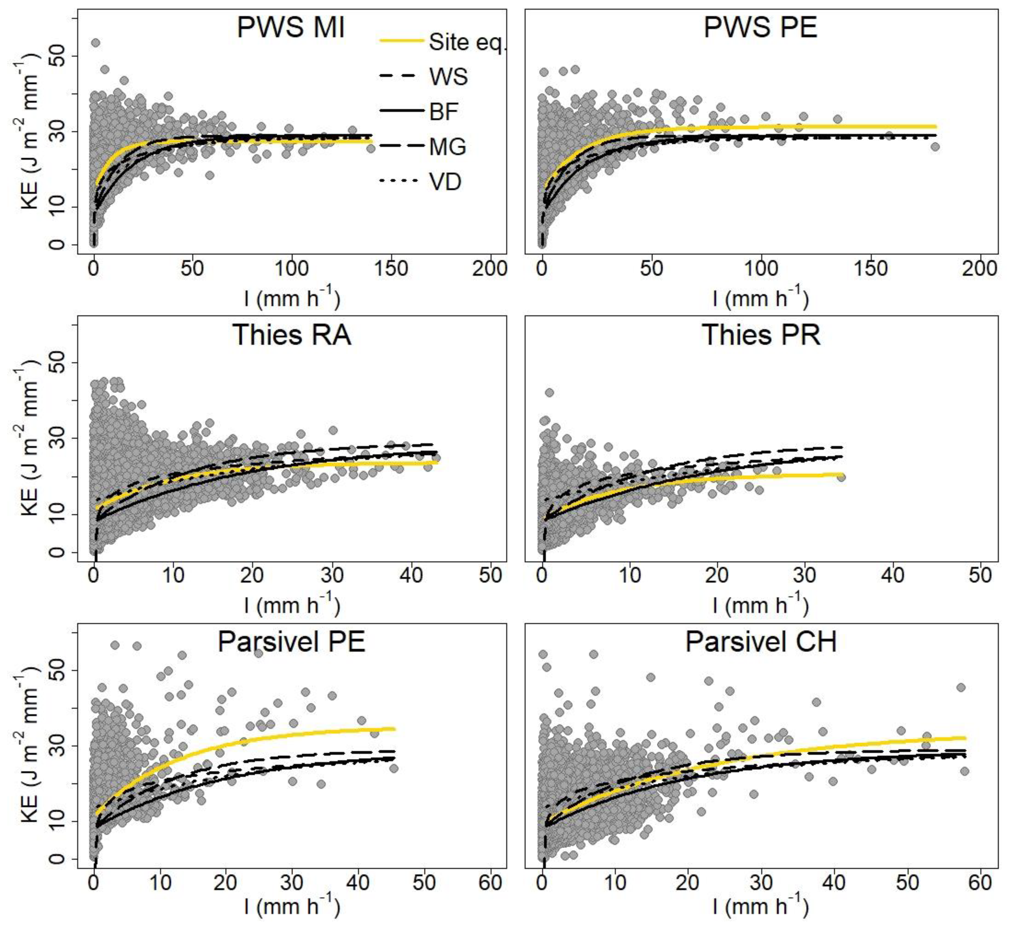
The KE per unit time (KE=J m−2 h−1) as used in the KE–I relationship here is related to the KE per unit rainfall (KE=J m−2 mm−1) through the rain intensity [65]. For clarity of comparison of the shape of the curves, the KE has been converted to KE per unit rainfall in Figure 4. It can be seen that the PWS MI curve reaches its maximum KE at lower intensities than the other equations. This behavior is determined by the c parameter of the equation, which defines the general shape of the curve [15]. As PWS MI has a higher value of c the curve reaches its max KE faster. The lowest value of c is found in the relationship for Parsivel CH, and it is clearly seen that the curve for this relationship only gradually reaches its max KE value at higher intensities.
3.4. Comparison with Rainfall Kinetic Energy–Intensity Relationships from the Literature
The KE sum of all analyzed rainfall minutes measured by the disdrometer, was compared to that found by inserting the disdrometer intensities into the four literature KE–I relationships (Table 1). The results presented in Table 5 show that there was no one KE-I relationship that fit the best at all sites. For PWS MI, the lowest percent bias of the four literature KE–I relationships was from WS, which underestimated KE from the disdrometer by 8.3%. For PWS PE the lowest PBIAS resulted from the VD equation with −6.6%. For Thies RA the WS had the lowest PBIAS of 5.8%. The BF equation gave the nearest fit to the Thies PR data with a PBIAS of −2.1%. Parsivel PE agreed the most with VD with a PBIAS of −4.6%, while Parsivel CH had the lowest PBIAS of 2.3% by MG. The site-specific relationships were calibrated on these data, so the error parameters show how well the calibration of the relationship was.
The only consistent trend was that BF always underestimated the total KE with PBIAS ranging from −2.1% to −30.2%. Several other studies based on disdrometer data also found that BF underestimates KE [5,8,18,32,33,66]. Nearing et al. [22] stated that BF should not be used for erosivity calculations, as it underestimates KE, and recommended using WS or MG, as they give the best results. This was also found in the present study, where together with VD these relationships gave good results for most datasets. Contrary to all other sites, BF was the best fitting equation to the Thies PR data measured on all error parameters. From Figure 4 it can be seen that the data points for Thies PR generally cluster at a lower KE value than the other sites, which causes a better fit with the BF curve. Angulo-Martínez et al. [19] collected data from a Thies disdrometer in Spain and also found that Brown and Foster performed quite well at estimating total KE for their data.
Petan et al. [5] measured KE at two sites in Slovenia, one equipped with a Parsivel and the other with a Thies disdrometer. They tested the agreement of the disdrometer KE with that found by the WS, BF and VD relationships and found similar percentage deviations for each relationship for both disdrometer types. However, they calculated drop velocity after Atlas et al. [50], so velocity differences between the devices had been eliminated.
3.5. Validation of Site-Specific Rainfall Kinetic Energy–Intensity Relationships on Rain Gauge Data
The new site-specific KE–I relationships developed from the PWS MI, PWS PE, Thies PR, Parsivel PE and Parsivel CH were tested by applying them to the intensities measured by rain gauges at the measurement sites and calculating daily KE and comparing it to the measured KE from the disdrometers (Figure 5). For all sites but CH, the rain gauges generally measured higher total daily rainfall amounts and KE than the disdrometers. The overall lowest deviation between disdrometer and rain gauge was found for PWS PE with a PBIAS of 6.2%. The rain gauge in PE was of the weighing type and these have been found to have higher accuracy than tipping buckets [67,68]. The highest deviation in daily rainfall amount was observed between Parsivel PE and the same rain gauge with a PBIAS of 39.7%, which suggests degraded performance of the disdrometer.
The lowest overall deviation of KE measured by a disdrometer and KE estimated with rain gauge intensity from the developed site-specific KE–I relationship was found for Parsivel CH. The underestimation of total daily rainfall amount also resulted in an underestimation of total daily KE with a PBIAS of −11.7%. The comparison between Parsivel PE and the rain gauge gave the highest overall deviation of daily KE with an overestimation of 104.2% by the rain gauge. This was expected due to the low agreement in rainfall amount measurements between Parsivel PE and the rain gauge.
Even though PWS PE showed the best agreement with the rain gauge, the KE was overestimated by 28.5% by the rain gauge. This may indicate that the developed KE–I relationship is prone to overestimation of KE. It may also suggest that rainfall intensity measurement between the PWS PE and the rain gauge may deviate more within events than can be seen from the daily comparison. This was shown by Johannsen et al. [43], who found that the rain gauge often measured higher intensities than four collocated disdrometers at the minute-scale.
Fraile et al. [37] observed lower rainfall amounts from a disdrometer than rain gauges and attributed this to the use of a standard measuring area. By using the effective measuring area, which decreases as the drop size increases, they found, that the rainfall amount measured by the disdrometer increased and generally became closer to that of the rain gauge. Other reasons, such as minimum rainfall resolution, smaller sampling area of the disdrometers compared to the rain gauges [39], exclusion of the smallest drop classes (Parsivel, [61]) or difference in drop size classification [69,70] may also affect the rainfall measurements. In addition, insufficient calibration of the tipping buckets may also have played a role, especially at the MI site, where an older model, which seems to have overestimated rainfall, was installed. However, these effects have not been explicitly investigated in the present study.
From these results, it is seen that the validation of the site-specific KE–I relationships using rain gauge data is only as good as the agreement between the rain gauge and disdrometer rainfall measurement. Depending on which rainfall measurement method is used, the KE estimates will vary due to differences in measured rainfall intensity and amount.
3.6. Implications of Disdrometer Differences for the Estimation of Rainfall Erosivity
The implication of the disdrometers measuring rainfall differently is that results are device-specific and therefore, the direct comparison of results from different disdrometer types is hindered. This can clearly be seen by the comparison of PWS PE and Parsivel PE, which were situated at the same site, but gave distinctive drop size and velocity distributions, which resulted in different KE–I relationships. This indicates that using one device instead of another may have a greater effect on the outcome of the developed KE–I relationship, than the local rainfall regime. For the formulation of the KE–I relationship, the PWS PE and Parsivel PE data did not cover exactly the same time period. Thus, a difference in measured rainfall events may explain some of the differences between the two devices. However, in Johannsen et al. [43], the KE–I relationships of the PWS100 and Parsivel disdrometers were established for the same rainfall events and were shown to differ due to instrumental differences.
In the present study, the actual measurement difference between the two disdrometers was quantified, by comparing the daily rainfall amount and KE for 27 rainy days, where both disdrometers measured more than 1 mm rainfall. The total rainfall amount measured by Parsivel PE was 26.0% lower than that measured by PWS PE and the MAE in rainfall amount was 2.7 mm. The total accumulated daily KE was also underestimated by Parsivel PE compared to PWS PE with 37.9% and a MAE of 65.3 J m−2. This deviation in measured rainfall amount and KE between devices placed at the same site shows the impact of the use of different disdrometers on the estimation of rainfall erosivity.
The sites Mistelbach and Rauchenwarth are within the same region of Austria and have similar average annual precipitation, and as such should not differ much in rainfall characteristics. However, due to the use of different devices, the drop size and velocity distributions, mean drop size and velocity and KE–I relationships found for these two sites were highly different. This shows the impact of using different devices under similar rainfall regimes.
On the other hand, data from the same type of disdrometer should be comparable, also when situated at different sites. As such, the results of PWS MI and PWS PE could enable comparison of the spatial differences in rainfall characteristics at the Mistelbach and Petzenkirchen sites. The comparison showed that mean drop size and velocity is larger in MI than in PE (Table 2). The maximum KE per rainfall unit is slightly lower for PWS MI, but the rise of the curve of the KE–I relationship reaches its maximum KE at lower intensities than that of PWS PE. This means, that at lower intensities (until the intersect of the curves), the KE calculated from the site-specific KE–I relationships is higher in Mistelbach than in Petzenkirchen.
The difference in raindrop measurement by the different disdrometers is related to the design and internal processing of each disdrometer. Variations in instrument measuring area, rainfall resolution, number of classes of drop size and velocity and built-in correction processes of drop measurement all affect the final rainfall measurements. The device-specific differences could be corrected for by calculating drop fall velocity from a terminal fall velocity equation [5,32,71], applying filters or correction schemes to the drop size distribution [38,41] or by applying a correction factor for KE between disdrometers [43]. However, this will not make results fully comparable and might introduce other biases. Thus, to have comparable results from multiple measurement sites, the same type of disdrometer should be used.
4. Conclusions
This study demonstrated that the rainfall erosivity estimation is influenced by the use of different types of rainfall measurement devices. Depending on the disdrometer type, rainfall was classified in a certain way, leading to distinctive drop size and velocity distributions for each disdrometer. Disdrometers of the same type, however, showed similarities in drop size and velocity distributions across the measurement sites. The drop sizes and velocities measured by the PWS100 disdrometers generally followed the terminal velocity line well. A large number of small drops with high velocities was measured by both Thies disdrometers and an overestimation of the velocity of smaller drops was measured by the two Parsivel disdrometers. The broad drop size and velocity distribution led to a scattered nature of the KE–I data points for the Thies and Parsivel disdrometers, which required a filtering of the data in order to develop new KE–I relationships.
Exponential KE–I relationships were developed for each site and disdrometer based on the filtered disdrometer data. The found parameters of the exponential relationship were different for each type of disdrometer and site.
The best fit of KE–I relationships from the literature (WS, BF, MG, VD) varied among disdrometers and sites. One universal KE–I relationship for all the sites could not be recommended. The BF relationship consistently underestimated KE compared to that measured by the disdrometers. Comparison with the literature KE-I relationships showed the importance of the site-specific disdrometer calibration as the percent bias of the relationships from literature was generally higher.
The site-specific KE–I relationships were successfully validated on rain gauge data, even though when rain gauge and disdrometer for any reason recorded different rainfall amount, the bias in KE estimation increased.
Results showed that, rainfall measurements by multiple types of disdrometers were associated with uncertainties stemming from instrumental differences. This led to variations in rainfall erosivity estimations between disdrometers even when placed at the same site. This was seen by the large percent bias in daily rainfall and KE measured by the PWS100 and Parsivel placed at the same site. Therefore, various disdrometers should not be used for comparison of the rainfall characteristics of different sites, as this will hinder the determination of spatial differences. If the use of the same type of disdrometer is not possible, or when comparing results from several studies, the possible effect of the specific disdrometer on the results must be recognized.
From our results, we cannot conclude which disdrometer type is better for rainfall measurements. Further research with methods such as artificial rainfall simulators with well-defined rainfall characteristics or the implementation of e.g., video disdrometers could help compare disdrometers to a certain reference and eliminate some of the uncertainties in rainfall erosivity estimation between instruments.
Author Contributions
Conceptualization, L.L.J. and A.K.; Formal analysis, L.L.J.; Funding acquisition, P.S., T.D. and A.K.; Investigation, L.L.J., N.Z. and M.N.; Methodology, L.L.J. and A.K.; Project administration, T.D. and A.K.; Supervision, P.S., T.D. and A.K.; Visualization, L.L.J.; Writing—original draft, L.L.J.; Writing—review and editing, All authors. All authors have read and agreed to the published version of the manuscript.
Funding
This research was performed within the project “Kinetic energy of rainfall as a driving force of soil detachment and transport”. Financial support was provided through the Austrian Science Fund (FWF): I 3049-N29 and the Czech Science Foundation (GACR): GF17-33751L. Open Access Funding by the Austrian Science Fund (FWF).
Acknowledgments
The disdrometer data from the Rauchenwarth site was provided by Austro Control Österreichische Gesellschaft für Zivilluftfahrt mbH.
Conflicts of Interest
The authors declare no conflict of interest.
References
- Montanarella, L.; Pennock, D.J.; McKenzie, N.; Badraoui, M.; Chude, V.; Baptista, I.; Mamo, T.; Yemefack, M.; Aulakh, M.S.; Yagi, K.; et al. World’s soils are under threat. Soil 2016, 2, 79–82. [Google Scholar] [CrossRef] [Green Version]
- Wischmeier, W.H.; Smith, D.D. Rainfall energy and its relationship to soil loss. Trans. Am. Geophys. Union 1958, 39, 285–291. [Google Scholar] [CrossRef]
- Sempere Torres, D.; Salles, C.; Creutin, J.D.; Delrieu, G. Quantification of soil detachment by raindrop impact: performance of classical formulae of kinetic energy in Mediterranean storms. In Erosion and Sediment Transport Monitoring Programmes in River Basins; The International Association of Hydrological Sciences: Wallingford, UK, 1992; pp. 115–124. [Google Scholar]
- Usón, A.; Ramos, M.C. An improved rainfall erosivity index obtained from experimental interrill soil losses in soils with a mediterranean climate. Catena 2001, 43, 293–305. [Google Scholar] [CrossRef]
- Petan, S.; Rusjan, S.; Vidmar, A.; Mikoš, M. The rainfall kinetic energy–intensity relationship for rainfall erosivity estimation in the mediterranean part of Slovenia. J. Hydrol. 2010, 391, 314–321. [Google Scholar] [CrossRef]
- Fornis, R.L.; Vermeulen, H.R.; Nieuwenhuis, J.D. Kinetic energy-rainfall intensity relationship for Central Cebu, Philippines for soil erosion studies. J. Hydrol. 2005, 300, 20–32. [Google Scholar] [CrossRef]
- Rosewell, C.J. Rainfall Kinetic Energy in Eastern Australia. J. Clim. Appl. Meteorol. 1986, 25, 1695–1701. [Google Scholar] [CrossRef] [Green Version]
- Coutinho, M.A.; Tomás, P.P. Characterization of raindrop size distributions at the Vale Formoso Experimental Erosion Center. Catena 1995, 25, 187–197. [Google Scholar] [CrossRef]
- Brandt, C.J. Simulation of the size distribution and erosivity of raindrops and throughfall drops. Earth Surf. Process. Landf. 1990, 15, 687–698. [Google Scholar] [CrossRef]
- Wischmeier, W.H.; Smith, D.D. Predicting Rainfall Erosion Losses—A Guide to Conservation Planning; U.S. Department of Agriculture: Washington, DC, USA, 1978.
- Shin, S.S.; Park, S.D.; Choi, B.K. Universal power law for relationship between rainfall kinetic energy and rainfall intensity. Adv. Meteorol. 2016, 2016, 1–11. [Google Scholar] [CrossRef] [Green Version]
- Smith, J.A.; De Veaux, R.D. The temporal and spatial variability of rainfall power. Environmetrics 1992, 3, 29–53. [Google Scholar] [CrossRef]
- Sanchez-Moreno, J.F.; Mannaerts, C.M.; Jetten, V.; Löffler-Mang, M. Rainfall kinetic energy-intensity and rainfall momentum-intensity relationships for Cape Verde. J. Hydrol. 2012, 454–455, 131–140. [Google Scholar] [CrossRef]
- Lim, Y.S.; Kim, J.K.; Kim, J.W.; Park, B.I.; Kim, M.S. Analysis of the relationship between the kinetic energy and intensity of rainfall in Daejeon, Korea. Quat. Int. 2015, 384, 107–117. [Google Scholar] [CrossRef]
- Van Dijk, A.I.J.M.; Bruijnzeel, L.A.; Rosewell, C.J. Rainfall intensity-kinetic energy relationships: A critical literature appraisal. J. Hydrol. 2002, 261, 1–23. [Google Scholar] [CrossRef]
- Brown, L.C.; Foster, G.R. Storm erosivity using idealized intensity distributions. Trans. ASAE 1987, 30, 379–386. [Google Scholar] [CrossRef]
- Kinnell, P.I.A. Rainfall Intensity-Kinetic Energy Relationships for Soil Loss Prediction. Soil Sci. Soc. Am. J. 1981, 45, 153. [Google Scholar] [CrossRef]
- Nanko, K.; Moskalski, S.M.; Torres, R. Rainfall erosivity-intensity relationships for normal rainfall events and a tropical cyclone on the US southeast coast. J. Hydrol. 2016, 534, 440–450. [Google Scholar] [CrossRef] [Green Version]
- Angulo-Martínez, M.; Beguería, S.; Kyselý, J. Use of disdrometer data to evaluate the relationship of rainfall kinetic energy and intensity (KE-I). Sci. Total Environ. 2016, 568, 83–94. [Google Scholar] [CrossRef] [Green Version]
- Meshesha, D.T.; Tsunekawa, A.; Haregeweyn, N. Influence of raindrop size on rainfall intensity, kinetic energy, and erosivity in a sub-humid tropical area: A case study in the northern highlands of Ethiopia. Theor. Appl. Climatol. 2019, 136, 1221–1231. [Google Scholar] [CrossRef]
- McGregor, K.C.; Bingner, R.L.; Bowie, A.J.; Foster, G.R. Erosivity index values for northern Mississippi. Trans. ASAE (Am. Soc. Agric. Eng.) 1995, 38, 1039–1047. [Google Scholar] [CrossRef]
- Nearing, M.A.; Yin, S.Q.; Borrelli, P.; Polyakov, V.O. Rainfall erosivity: An historical review. Catena 2017, 157, 357–362. [Google Scholar] [CrossRef]
- Klik, A.; Haas, K.; Dvorackova, A.; Fuller, I.C. Spatial and temporal distribution of rainfall erosivity in New Zealand. Soil Res. 2015, 53, 815–825. [Google Scholar] [CrossRef]
- Panagos, P.; Ballabio, C.; Borrelli, P.; Meusburger, K.; Klik, A.; Rousseva, S.; Perčec Tadić, M.; Michaelides, S.; Hrabalíková, M.; Olsen, P.; et al. Rainfall erosivity in Europe. Sci. Total Environ. 2015, 511C, 801–814. [Google Scholar] [CrossRef] [PubMed] [Green Version]
- Xie, Y.; Yin, S.Q.; Liu, B.Y.; Nearing, M.A.; Zhao, Y. Models for estimating daily rainfall erosivity in China. J. Hydrol. 2016, 535, 547–558. [Google Scholar] [CrossRef] [Green Version]
- Panagos, P.; Borrelli, P.; Meusburger, K.; Yu, B.; Klik, A.; Lim, K.J.; Yang, J.E.; Ni, J.; Miao, C.; Chattopadhyay, N.; et al. Global rainfall erosivity assessment based on high-temporal resolution rainfall records. Sci. Rep. 2017, 7, 1–12. [Google Scholar] [CrossRef] [PubMed] [Green Version]
- Panagos, P.; Ballabio, C.; Meusburger, K.; Spinoni, J.; Alewell, C.; Borrelli, P. Towards estimates of future rainfall erosivity in Europe based on REDES and WorldClim datasets. J. Hydrol. 2017, 548, 251–262. [Google Scholar] [CrossRef]
- Wilken, F.; Baur, M.; Sommer, M.; Deumlich, D.; Bens, O.; Fiener, P. Uncertainties in rainfall kinetic energy-intensity relations for soil erosion modelling. Catena 2018, 171, 234–244. [Google Scholar] [CrossRef]
- Lobo, G.P.; Bonilla, C.A. Sensitivity analysis of kinetic energy-intensity relationships and maximum rainfall intensities on rainfall erosivity using a long-term precipitation dataset. J. Hydrol. 2015, 527, 788–793. [Google Scholar] [CrossRef]
- Cerro, C.; Bech, J.; Codina, B.; Lorente, J. Modeling Rain Erosivity Using Disdrometric Techniques. Soil Sci. Soc. Am. J. 1998, 62, 731–735. [Google Scholar] [CrossRef]
- Jayawardena, A.W.; Rezaur, R.B. Drop size distribution and kinetic energy load of rainstorms in Hong Kong. Hydrol. Process. 2000, 14, 1069–1082. [Google Scholar] [CrossRef]
- Angulo-Martínez, M.; Barros, A.P.P. Measurement uncertainty in rainfall kinetic energy and intensity relationships for soil erosion studies: An evaluation using PARSIVEL disdrometers in the Southern Appalachian Mountains. Geomorphology 2015, 228, 28–40. [Google Scholar] [CrossRef]
- Ramon, R.; Minella, J.P.G.; Merten, G.H.; de Barros, C.A.P.; Canale, T. Kinetic energy estimation by rainfall intensity and its usefulness in predicting hydrosedimentological variables in a small rural catchment in southern Brazil. Catena 2017, 148, 176–184. [Google Scholar] [CrossRef]
- Grossklaus, M.; Uhlig, K.; Hasse, L. An optical disdrometer for use in high wind speeds. J. Atmos. Ocean. Technol. 1998, 15, 1051–1059. [Google Scholar] [CrossRef]
- de Moraes Frasson, R.P.; da Cunha, L.K.; Krajewski, W.F. Assessment of the Thies optical disdrometer performance. Atmos. Res. 2011, 101, 237–255. [Google Scholar] [CrossRef]
- Battaglia, A.; Rustemeier, E.; Tokay, A.; Blahak, U.; Simmer, C. PARSIVEL Snow Observations: A Critical Assessment. J. Atmos. Ocean. Technol. 2010, 27, 333–344. [Google Scholar] [CrossRef]
- Fraile, R.; Castro, A.; Fernández-Raga, M.; Palencia, C.; Calvo, A.I. Error in the sampling area of an optical disdrometer: Consequences in computing rain variables. Sci. World J. 2013, 2013. [Google Scholar] [CrossRef]
- Angulo-Martínez, M.; Beguería, S.; Latorre, B.; Fernández-Raga, M. Comparison of precipitation measurements by OTT Parsivel2 and Thies LPM optical disdrometers. Hydrol. Earth Syst. Sci. 2018, 22, 2811–2837. [Google Scholar] [CrossRef] [Green Version]
- Krajewski, W.F.; Kruger, A.; Caracciolo, C.; Golé, P.; Barthes, L.; Creutin, J.-D.; Delahaye, J.-Y.; Nikolopoulos, E.I.; Ogden, F.; Vinson, J.-P. DEVEX-disdrometer evaluation experiment: Basic results and implications for hydrologic studies. Adv. Water Resour. 2006, 29, 311–325. [Google Scholar] [CrossRef]
- Liu, X.C.; Gao, T.C.; Liu, L. A comparison of rainfall measurements from multiple instruments. Atmos. Meas. Tech. 2013, 6, 1585–1595. [Google Scholar] [CrossRef] [Green Version]
- Raupach, T.H.; Berne, A. Correction of raindrop size distributions measured by Parsivel disdrometers, using a two-dimensional video disdrometer as a reference. Atmos. Meas. Tech. 2015, 8, 343–365. [Google Scholar] [CrossRef] [Green Version]
- Tokay, A.; Petersen, W.A.; Gatlin, P.; Wingo, M. Comparison of Raindrop Size Distribution Measurements by Collocated Disdrometers. J. Atmos. Ocean. Technol. 2013, 30, 1672–1690. [Google Scholar] [CrossRef]
- Johannsen, L.L.; Zambon, N.; Strauss, P.; Dostal, T.; Neumann, M.; Zumr, D.; Cochrane, T.A.; Blöschl, G.; Klik, A. Comparison of three types of laser optical disdrometers under natural rainfall conditions. Hydrol. Sci. J. 2020, 65, 524–535. [Google Scholar] [CrossRef]
- Land Niederösterreich. Wasserstandsnachrichten und Hochwasserprognosen. Messstellendaten. Mistelbach. Available online: https://www.noe.gv.at/wasserstand/#/de/Messstellen/Details/99116541/Niederschlag/3Tage (accessed on 25 November 2019).
- Land Niederösterreich. Wasserstandsnachrichten und Hochwasserprognosen. Messstellendaten. Wieselburg. Available online: https://www.noe.gv.at/wasserstand/#/de/Messstellen/Details/107235/Niederschlag/3Tage (accessed on 25 November 2019).
- ZAMG. Klimadaten von Österreich 1971-2000: Schwechat. Available online: http://www.zamg.ac.at/fix/klima/oe71-00/klima2000/klimadaten_oesterreich_1971_frame1.htm (accessed on 25 November 2019).
- Czech Hydrometeorological Institute. Prague Clementinum: Basic data on Prague Clementinum Station. Available online: http://portal.chmi.cz/historicka-data/pocasi/praha-klementinum?l=en# (accessed on 25 November 2019).
- NIWA Climate Summaries. Available online: https://niwa.co.nz/education-and-training/schools/resources/climate/summary (accessed on 25 November 2019).
- World Meteorological Organization (WMO). Manual on Codes—International Codes, Volume I.1, Annex II to the WMO Technical Regulations: Part A—Alphanumeric Codes; World Meteorological Organization: Geneva, Switzerland, 2011. [Google Scholar]
- Atlas, D.; Srivastava, R.C.; Sekhon, R.S. Doppler Radar Characteristics of Precipitation at Vertical Incidence. Rev. Geophys. 1973, 11, 1–35. [Google Scholar] [CrossRef]
- Adirosi, E.; Roberto, N.; Montopoli, M.; Gorgucci, E.; Baldini, L. Influence of disdrometer type on weather radar algorithms from measured DSD: Application to Italian climatology. Atmosphere (Basel) 2018, 9, 360. [Google Scholar] [CrossRef] [Green Version]
- Jaffrain, J.; Berne, A. Experimental quantification of the sampling uncertainty associated with measurements from PARSIVEL disdrometers. J. Hydrometeorol. 2011, 12, 352–370. [Google Scholar] [CrossRef]
- Kruger, A.; Krajewski, W.F. Two-Dimensional Video Disdrometer: A Description. J. Atmos. Ocean. Technol. 2002, 19, 602–617. [Google Scholar] [CrossRef]
- Tokay, A.; Kruger, A.; Krajewski, W.F. Comparison of drop size distribution measurements by impact and optical disdrometers. J. Appl. Meteorol. 2001, 40, 2083–2097. [Google Scholar] [CrossRef]
- Hauser, D.; Amayenc, P.; Nutten, B.; Waldteufel, P. A New Optical Instrument for Simultaneous Measurement of Raindrop Diameter and Fall Speed Distributions. J. Atmos. Ocean. Technol. 1984, 1, 256. [Google Scholar] [CrossRef]
- Donnadieu, G. Comparison of results obtained with the VIDIAZ spectropluviometer and the Joss-Waldvogel rainfall disdrometer in a “rain of a thundery type”. J. Appl. Meteorol. 1980, 19, 593–597. [Google Scholar] [CrossRef]
- Renard, K.G.; Foster, G.R.; Weesies, G.A.; McCool, D.K.; Yoder, D.C. Predicting Soil Erosion by Water: A Guide to Conservation Planning With the Revised Universal Soil Loss Equation (RUSLE); U.S. Department of Agriculture, Agricultural Research Service: Washington, DC, USA, 1997.
- Bates, D.M.; Watts, D.G. Nonlinear Regression Analysis and Its Applications. In Wiley Series in Probability and Statistics, Bates, D.M., Watts, D.G., Eds.; John Wiley & Sons, Inc.: Hoboken, NJ, USA, 1988. [Google Scholar]
- R Core Team. R: A Language and Environment for Statistical Computing; R Foundation for Statistical Computing: Vienna, Austria, 2018. [Google Scholar]
- Tokay, A.; Wolff, D.B.; Petersen, W.A. Evaluation of the New Version of the Laser-Optical Disdrometer, OTT Parsivel 2. J. Atmos. Ocean. Technol. 2014, 31, 1276–1288. [Google Scholar] [CrossRef]
- OTT. Operating Instructions. Present Weather Sensor Parsivel; OTT Messtechnik GmbH & Co. KG.: Kempten, Germany, 2005. [Google Scholar]
- Thies Clima. Instruction for Use. Laser Precipitation Monitor; Adolf Thies GmbH & Co. KG.: Göttingen, Germany, 2015. [Google Scholar]
- Campbell Scientific Inc. PWS100 Present Weather Sensor. Instruction manual. Revision 3/12; Campbell Scientific, Inc.: Logan, UT, USA, 2012. [Google Scholar]
- Montero-Martínez, G.; García-García, F. On the behaviour of raindrop fall speed due to wind. Q. J. R. Meteorol. Soc. 2016, 142, 2013–2020. [Google Scholar] [CrossRef]
- Salles, C.; Poesen, J.; Sempere-Torres, D. Kinetic energy of rain and its functional relationship with intensity. J. Hydrol. 2002, 257, 256–270. [Google Scholar] [CrossRef]
- Mineo, C.; Ridolfi, E.; Moccia, B.; Russo, F.; Napolitano, F. Assessment of Rainfall Kinetic-Energy–Intensity Relationships. Water 2019, 11, 1994. [Google Scholar] [CrossRef] [Green Version]
- Lanza, L.G.; Vuerich, E. The WMO Field Intercomparison of Rain Intensity Gauges. Atmos. Res. 2009, 94, 534–543. [Google Scholar] [CrossRef]
- Michaelides, S.; Levizzani, V.; Anagnostou, E.; Bauer, P.; Kasparis, T.; Lane, J.E. Precipitation: Measurement, remote sensing, climatology and modeling. Atmos. Res. 2009, 94, 512–533. [Google Scholar] [CrossRef]
- Fraile, R.; Palencia, C.; Castro, A.; Giaiotti, D.; Stel, F. Fitting an exponential distribution: Effect of discretization. Atmos. Res. 2009, 93, 636–640. [Google Scholar] [CrossRef]
- Marzuki, M.; Randeu, W.L.; Schönhuber, M.; Bringi, V.N.; Kozu, T.; Shimomai, T. Raindrop size distribution parameters of distrometer data with different bin sizes. IEEE Trans. Geosci. Remote Sens. 2010, 48, 3075–3080. [Google Scholar] [CrossRef]
- Jaffrain, J.; Berne, A. Quantification of the small-scale spatial structure of the raindrop size distribution from a network of disdrometers. J. Appl. Meteorol. Climatol. 2012, 51, 941–953. [Google Scholar] [CrossRef]
Figure 1.
Disdrometers at the measurement sites Mistelbach (MI), Petzenkirchen (PE), Prague (PR) and Christchurch (CH) (a photo of the Thies Rauchenwarth (RA) site was not available).
Figure 1.
Disdrometers at the measurement sites Mistelbach (MI), Petzenkirchen (PE), Prague (PR) and Christchurch (CH) (a photo of the Thies Rauchenwarth (RA) site was not available).

Figure 2.
Drop size and velocity distribution for all disdrometers at each site. The color legend describes the percentage of drops in each drop size and velocity class as a percentage of the number of drops in the class with most drops. The black line is the terminal velocity line drawn after Atlas et al. [50]. Drops in classes outside the red lines deviate more than 50% from the terminal velocity line.

Figure 3.
Rainfall kinetic energy–intensity relationships for each disdrometer and site with both unfiltered and filtered data points shown. The black line is the developed exponential rainfall kinetic energy–intensity relationship. Notes: MI = Mistelbach; PE = Petzenkirchen; RA = Rauchenwarth; PR = Prague; and CH = Christchurch.

Figure 4.
Rainfall kinetic energy per unit area and unit rainfall plotted against rainfall intensity for each disdrometer and site, and comparison of the developed rainfall kinetic energy–intensity relationships and the rainfall kinetic energy–intensity relationships Wischmeier and Smith (WS); Brown and Foster (BF); McGregor et al. (MG); and van Dijk et al. (VD) from the literature. Notes: MI = Mistelbach; PE = Petzenkirchen; RA = Rauchenwarth; PR = Prague; and CH = Christchurch.

Figure 5.
Rain gauge (RG) and disdrometer comparison of daily rainfall and rainfall kinetic energy for the sites Mistelbach (MI), Petzenkirchen (PE), Prague (PR) and Christchurch (CH).
Figure 5.
Rain gauge (RG) and disdrometer comparison of daily rainfall and rainfall kinetic energy for the sites Mistelbach (MI), Petzenkirchen (PE), Prague (PR) and Christchurch (CH).


Table 1.
Relationships between kinetic energy, KE (J m−2 h−1) and intensity, I (mm h−1).
| Reference | Equation | Abbreviation |
|---|---|---|
| Wischmeier and Smith [10] | , I ≤ 76 mm h−1 | WS |
| , I > 76 mm h−1 | ||
| Brown and Foster [16] | BF | |
| McGregor et al. [21] | MG | |
| van Dijk et al. [15] | VD |
Table 2.
Measurement site characteristics and disdrometer types.
| Measurement Site | Coordinates | Altitude | Mean Annual Precipitation | Mean Annual Temperature | Disdrometer Type |
|---|---|---|---|---|---|
| (m.a.s.l.) | (mm) | (°C) | |||
| Mistelbach | 48°34′59″ N, 16°35′14″ E | 245 | 537 | 9.8 | PWS100 |
| Petzenkirchen | 48°09′17″ N, 15°08′53″ E | 277 | 902 | 9.6 | PWS100 and Parsivel |
| Rauchenwarth | 48°05′ N, 16°32′ E | 210 | 533 | 9.8 | Thies |
| Prague | 50°06′16″ N, 14°23′14″ E | 230 | 459 | 10.8 | Thies |
| Christchurch | 43°31′18″ S, 172°34′59″ E | 24 | 648 | 12.1 | Parsivel |
Table 3.
Mean drop size and velocity (± standard deviation) before and after filtering.
| Before Filtering | After Filtering | |||
|---|---|---|---|---|
| Device and Site | Mean Size | Mean Velocity | Mean Size | Mean Velocity |
| (mm) | (m s−1) | (mm) | (m s−1) | |
| PWS MI | 1.2 (±0.3) | 4.3 (±2.7) | 1.2 (±0.3) | 4.3 (±2.5) |
| PWS PE | 0.9 (±0.2) | 3.7 (±1.9) | 1.0 (±0.2) | 3.7 (±1.9) |
| Thies RA | 0.4 (±0.1) | 2.0 (±2.4) | 0.6 (±0.1) | 2.0 (±1.6) |
| Thies PR | 0.6 (±0.1) | 2.3 (±1.5) | 0.7 (±0.2) | 2.4 (±1.5) |
| Parsivel PE | 0.7 (±0.1) | 4.0 (±0.7) | 0.9 (±0.1) | 4.2 (±0.8) |
| Parsivel CH | 0.6 (±0.1) | 3.2 (±1.3) | 0.8 (±0.1) | 3.1 (±1.3) |
Notes: MI = Mistelbach; PE = Petzenkirchen; RA = Rauchenwarth; PR = Prague; and CH = Christchurch.
Table 4.
Specifics of data from each measurement site and the developed rainfall kinetic energy–intensity relationships after filtering.
Table 4.
Specifics of data from each measurement site and the developed rainfall kinetic energy–intensity relationships after filtering.
| Disdrometer and Site | Rainfall Kinetic Energy–Intensity Relationship (J m−2 h−1) | R2 | Minutes Analyzed | Total Rain (mm) |
|---|---|---|---|---|
| PWS MI | 27.4·I·(1−0.49·e−0.121·I) | 0.98 | 18001 | 582 |
| PWS PE | 31.2·I·(1−0.55·e−0.057·I) | 0.97 | 85605 | 1255 |
| Thies RA | 23.6·I·(1−0.53·e−0.103·I) | 0.95 | 152284 | 1397 |
| Thies PR | 20.6·I·(1−0.57·e−0.111·I) | 0.96 | 15708 | 190 |
| Parsivel PE | 35.0·I·(1−0.68·e−0.079·I) | 0.91 | 19059 | 181 |
| Parsivel CH | 34.0·I·(1−0.72·e−0.043·I) | 0.90 | 47058 | 787 |
Notes: MI = Mistelbach; PE = Petzenkirchen; RA = Rauchenwarth; PR = Prague; and CH = Christchurch.
Table 5.
Comparison of the measured rainfall kinetic energy to that found from the calibration of the site- and device-specific rainfall kinetic energy–intensity relationships and the rainfall kinetic energy–intensity relationships Wischmeier and Smith (WS); Brown and Foster (BF); McGregor et al. (MG); and van Dijk et al. (VD) from the literature.
| Disdrometer and Measurement Site | Rainfall Kinetic Energy–Intensity Relationship | Sum KE (J m−2) | PBIAS (%) | RMSE (J m−2) | MAE (J m−2) |
|---|---|---|---|---|---|
| PWS MI | Measured | 12719 | |||
| Site-specific relationship | 12956 | 1.9 | 0.393 | 0.117 | |
| WS | 11657 | −8.3 | 0.482 | 0.150 | |
| BF | 10108 | −20.5 | 0.515 | 0.171 | |
| MG | 11293 | −11.2 | 0.427 | 0.134 | |
| VD | 11409 | −10.3 | 0.463 | 0.127 | |
| PWS PE | Measured | 22807 | |||
| Site-specific relationship | 23566 | 3.3 | 0.219 | 0.054 | |
| WS | 20614 | −9.5 | 0.295 | 0.070 | |
| BF | 16899 | −25.9 | 0.294 | 0.077 | |
| MG | 19004 | −16.7 | 0.246 | 0.064 | |
| VD | 21311 | −6.6 | 0.273 | 0.057 | |
| Thies RA | Measured | 19174 | |||
| Site-specific relationship | 20194 | 5.3 | 0.102 | 0.033 | |
| WS | 20244 | 5.8 | 0.135 | 0.049 | |
| BF | 15919 | −17.0 | 0.123 | 0.036 | |
| MG | 18020 | −6.0 | 0.116 | 0.032 | |
| VD | 21777 | 13.6 | 0.104 | 0.038 | |
| Thies PR | Measured | 2273 | |||
| Site-specific relationship | 2356 | 3.6 | 0.096 | 0.035 | |
| WS | 2819 | 24.2 | 0.175 | 0.065 | |
| BF | 2225 | −2.1 | 0.108 | 0.035 | |
| MG | 2524 | 11.0 | 0.153 | 0.040 | |
| VD | 2997 | 31.8 | 0.129 | 0.056 | |
| Parsivel PE | Measured | 2968 | |||
| Site-specific relationship | 2966 | −0.1 | 0.219 | 0.037 | |
| WS | 2526 | −14.6 | 0.305 | 0.053 | |
| BF | 2071 | −30.2 | 0.296 | 0.051 | |
| MG | 2313 | −22.1 | 0.254 | 0.043 | |
| VD | 2831 | −4.6 | 0.280 | 0.043 | |
| Parsivel CH | Measured | 10713 | |||
| Site-specific relationship | 10799 | 0.8 | 0.237 | 0.064 | |
| WS | 12408 | 16.0 | 0.300 | 0.094 | |
| BF | 9565 | −10.7 | 0.251 | 0.062 | |
| MG | 10954 | 2.3 | 0.243 | 0.064 | |
| VD | 12640 | 18.0 | 0.256 | 0.078 |
Notes: MI = Mistelbach; PE = Petzenkirchen; RA = Rauchenwarth; PR = Prague; and CH = Christchurch.
© 2020 by the authors. Licensee MDPI, Basel, Switzerland. This article is an open access article distributed under the terms and conditions of the Creative Commons Attribution (CC BY) license (http://creativecommons.org/licenses/by/4.0/).
Share and Cite
MDPI and ACS Style
Johannsen, L.L.; Zambon, N.; Strauss, P.; Dostal, T.; Neumann, M.; Zumr, D.; Cochrane, T.A.; Klik, A. Impact of Disdrometer Types on Rainfall Erosivity Estimation. Water 2020, 12, 963. https://doi.org/10.3390/w12040963
AMA Style
Johannsen LL, Zambon N, Strauss P, Dostal T, Neumann M, Zumr D, Cochrane TA, Klik A. Impact of Disdrometer Types on Rainfall Erosivity Estimation. Water. 2020; 12(4):963. https://doi.org/10.3390/w12040963
Chicago/Turabian StyleJohannsen, Lisbeth Lolk, Nives Zambon, Peter Strauss, Tomas Dostal, Martin Neumann, David Zumr, Thomas A. Cochrane, and Andreas Klik. 2020. "Impact of Disdrometer Types on Rainfall Erosivity Estimation" Water 12, no. 4: 963. https://doi.org/10.3390/w12040963
Note that from the first issue of 2016, this journal uses article numbers instead of page numbers. See further details here.