A Computational Fluid Dynamics Simulation Model of Sediment Deposition in a Storage Reservoir Subject to Water Withdrawal


Department of Civil, Environmental and Natural Resources Engineering, Luleå University of Technology, 971 87 Luleå, Sweden
*
Author to whom correspondence should be addressed.
Water 2020, 12(4), 959; https://doi.org/10.3390/w12040959
Submission received: 23 February 2020
/
Revised: 19 March 2020
/
Accepted: 24 March 2020
/
Published: 28 March 2020
(This article belongs to the Section Hydrology)
Abstract
:Siltation is one of the most common problems in storage projects and attached structures around the world, due to its effects on a project’s life span and operational efficiency. A three-dimensional computational fluid dynamics (CFD) model was applied to study the flow and sediment deposition in a multipurpose reservoir (Mosul Dam Reservoir, Iraq) subject to water withdrawal via a pumping station. A suitable control code was developed for the sediment simulation in intakes with multiblock option (SSIIM) model, in order to simulate a study case and achieve the study aims. The measured total deposited load in the reservoir after 25 years of operation and the measured sediment load concentration at different points near the pumping station intake were considered to validate the model results. The sediment load concentrations at several points near the water intake were compared; the percent bias (PBIAS) value was 3.6%, while the t-test value was 0.43, less than the tabulated value, indicating fair model performance. The model sensitivity to grid size and time steps was also tested. Four selected bed level sections along the reservoir were compared with the simulated values and indicate good performance of the model in predicting the sediment load deposition. The PBIAS ranged between 4.8% and 80.7%, and the paired t-test values indicate good model performance for most of the sections.
1. Introduction
Usually, the flow regime in rivers balances the sediment transportation between the flow transport capacity and sediment load concentration. The construction of different hydraulic structures, such as barrages, weirs, and dams, for different purposes (e.g., storage, flood control, power generation, and multipurpose dams) changes this balance. In dam reservoirs, the gradual expansion of the flow section when the flow approaches the reservoir inlet leads to sediment load deposition that is coarser and then finer toward the flow direction. After years of dam operation, the sediment deposition leads to a reduction in storage capacity, in addition to its effects on the operational efficiency of different hydraulic structures attached to the project, such as bottom outlet gates, hydropower plants, and different water intakes with different purposes. One of the most important factors that should be considered in dam construction and operation schedules is the sustainability of such structures. Sustainability approaches for a reservoir’s life span and operational efficiency should include a plan for sediment control by direct estimation, to reduce its effects or provide sufficient funds to treat its effects later [1]. The assessment and control of sediment yield through catchment is one of the common approaches to reduce its effects. Several previous studies have been concerned about soil erosion assessment and control. The authors of [2] estimated the hydrologic and erosion variation due to vineyards’ planting effects under the simulated rainfall. The planting causes an increase in the topsoil bulk density, reduces surface roughness, and causes an increase in runoff and non-sustainable soil losses. The results show the importance of finding a suitable approach to reduce the soil loss during the plantation period. Other authors [3,4] have evaluated the effect of using a straw mulch on soil loss control, using rainfall simulator plots and field plots in Spain. The results showed that there was a reduction in both runoff and soil erosion, and the combination of both straw and no tillage reduces the sediment yield. The effects of sedimentation on a reservoir’s storage capacity and operational efficiency leads to reductions in benefits compared to operational costs. An underestimation of the sediment load or unexpected sediment deposition leads to a reduction in the project’s life span or the dam’s operational efficiency and capacity. In addition to the effect of soil erosion on reservoirs’ storage capacity, it also causes a loss of the upper fertilized soil layer. A reduction in agricultural activity was observed in different regions of Europe after the Second World War, due to different social and economic effects [5]; changes in water and sediment yield, as well as deposition rate for the Dragonja catchment in southwestern Slovenia were studied. The results indicate that the main sources of sediments are hillslopes, erosional bedrock banks, and sedimentary riverbanks. The hillslopes have a high percentage of sediment yield contribution. Chipped pruned branches (CBRs) were used to evaluate their effect on improving soil quality [6]. The results indicate that using CBRs increased organic matter and reduced soil bulk density, which lead to a reduction in sediment concentration and rate of soil loss. Furthermore, the intakes, gates, and various attached dam structures were affected by underestimation of sediment load and deposition rate. The underestimation of sediment load and its deposition near the intakes and outlets of different structures may cause clogging and stop the structure from functioning. A fund is necessary in this case to keep or recover the cost–benefit values of the project. Suitable solutions in such cases are usually determined in one of two ways: physical laboratory models and numerical models. The high capacity and speed of modern computers have made numerical modelling, such as computational fluid dynamics (CFD) models for some cases of open channels flow, rivers, lakes, and different water bodies, applicable efficiently. In addition, the main advantages of using such models are their reduction in costs and time [7], in comparison to the physical models; however, the numerical models still cannot overcome obstacles in some complicated applications of flow and sediment studies. Such studies include scour around the piers and flow junctions and sluice gates scouring, as well as others that include turbulent flow. In such cases (turbulent flow), the numerical solution requires small-scale elements, and the direct solution in most cases is unfeasible, as quoted in [8]. Numerical models can be divided into one-, two-, and three-dimensional (1-D, 2-D, and 3-D, respectively) models. Depending on the purpose of the study, a suitable model can be selected. Generally, for a long-term simulation and the simulation of sediment transport along a reach, a 1-D model can achieve this purpose efficiently [9] with less input calibration data. On the other hand, 2-D and 3-D models are used to study sediment transportation and deposition when the purpose is to determine how sediment is distributed across the flow section, or at certain locations in reservoirs like gates, intakes, and power plant inlets. However, these models require more data and greater computing time.
A 3-D numerical model, sediment simulation in intakes with multiblock option (SSIIM2) was applied to study the sediment flushing in the steep bendy channel of the Dashidaira reservoir in Japan [10]. The complexity of this case is due to the interactions between unsteady flow and bed-level changes. Comparing the bed level before and after the flushing process was considered for model verification, and different bed load formulas were applied for the model sensitivity analysis. The sediment transport and deposition in the Hamidieh Reservoir in Iran, with special emphasis near the sluice gates and intakes, has been studied by applying a 3-D numerical model [11]. Different scenarios were applied to study the effects of the operational scheme on flow and sediment transportation for different intakes and sluice gate structures in the studied reservoir. The SSIIM model was applied to study the morphodynamic processes in the Iffezheim reservoir at the Upper Rhine River in Germany, in order to determine the accuracy of the model in a bed-level change simulation, as well as the sensitivity of the effective parameters [12]. A comparison between the model results and measured data indicates that the model’s performance is satisfactory. The SSIIM model was applied to the Angostura hydropower reservoir in Costa Rica to review the suspended load distribution and pattern of sediment deposition [13]. The 3-D measurements of the suspended load and grain size distribution at twenty-five locations in the considered vertical profiles were compared with the model results. A reasonable result for the comparison between the measured and simulated values was obtained for both the suspended load concentration and the bed level variation. The SSIIM model has been applied for modelling the sediment deposition and flushing process in different reservoirs [14,15,16,17]. For a long simulation period of the sedimentation in the reservoir (11 years), the SSIIM model was applied to predict the bed changes due to sedimentation and dredging [18]. The model sensitivity was tested for grid size, fall velocity, cohesion, and sediment transport formula. The deviation in sediment volume due to these parameters’ effect was less than 16%. The flow velocity, distribution, and reservoir storage level of the Jeziorsko Reservoir in Poland have been studied by using the SSIIM model [19]. The results of this applied model show that there are no significant differences to the measured flow velocity. One of the ways to describe and qualify the water and sediments flux is called connectivity [20], in which the authors present a short review of connectivity concepts and present a new method for the concept of connectivity to water and sediment flux. This approach presents a better understanding of water and sediment dynamics in comparison to previous approaches.
The siltation problem near and inside intakes and pumping stations has been studied using different numerical and physical models. The problem of sediment accumulation near and inside the intake structure of the North Al-Jazeera irrigation project in the Mosul Dam in Iraq has been studied [21]. This study included measurements of sediment depth near the intake, particle size distribution, and a few values for the flow velocity at selected sites.
The flow near the intake and suction pipe of the Dongsong pumping station in China has been simulated by the application of a 3-D model, using both the standard k–ε turbulence and the finite volume method to measure the design flow rate [22]. The problem of rapid accumulation of sediment near the intake structure of a high-head power plant in the Austrian Alps has been studied by using both a 3-D model (ANSYS-CFX) and a physical laboratory model to determine a reasonable solution [23]. The numerical 3-D simulation model was considered to simulate the complex geometry and find a new design for the trash rack. The siltation condition near the water intake in a storage reservoir in Morocco was studied; the study included developing a 2-D model to simulate the situation and analyse the effects of sediment on the intake’s operations [24]. The applied model indicates a possibility of station shutdown period prediction, with respect to the carried suspended load of heavy rainstorms.
The aims of this paper are to simulate the sediment transport, deposition, and morphological bed-level changes, with special attention to the areas neighboring the water intake in the reservoir, which are subject to water withdrawal, in order to determine its effect on sediment load distribution. The Mosul Dam reservoir and its pumping station, which are suffering from an accumulation of sediment near and inside the intake, was considered as a case study. The existence of the pumping station makes the flow regime and sediment transport more complicated, and only 2-D or 3-D models can describe or simulate this case. A control code for SSIIM2 model as a 3-D numerical model was prepared to simulate this situation.
2. Site Description
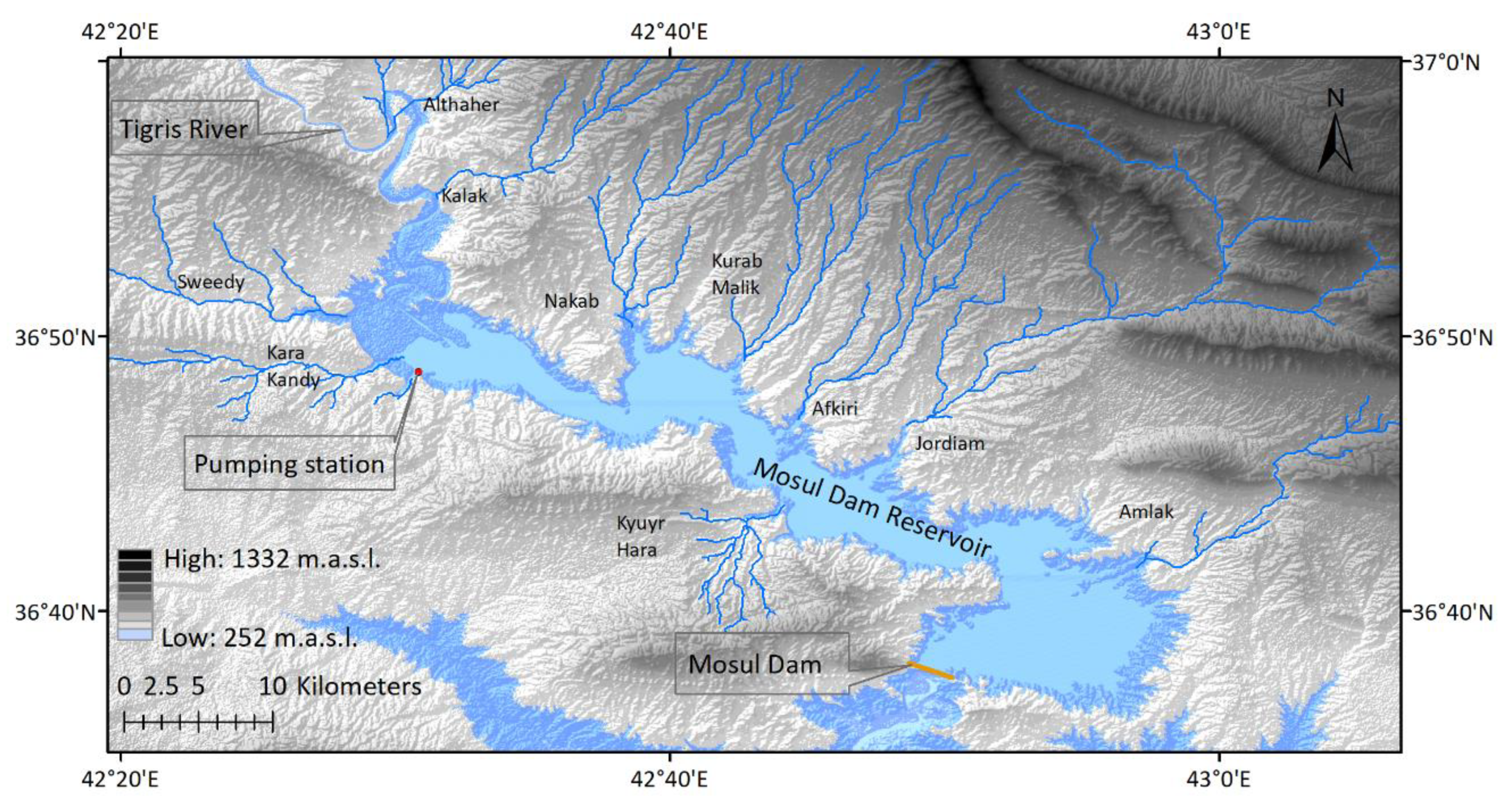
The pumping station in Mosul Dam was selected in this study. The Mosul Dam is a multipurpose dam located on the Tigris River, northern Iraq. The dam’s total storage capacity at the maximum operation level of 335 (m a.s.l.), is 11.11 × 10⁹ m3, including 2.95 × 10⁹ m3 as dead storage. The main inflow and sediment load that feeds the Mosul Dam reservoir is the Tigris River. In addition, there are ten seasonal valleys on both sides of the reservoir adding flow and sediment load, which makes the reservoir flow regime more complex (Figure 1), the topography, Digital Elevation Model (DEM) of the area was also shown in the figure. The average annual sediment load that was delivered to the Mosul Dam reservoir during the period 1986–2011 is about 48 × 106 m3 [25].
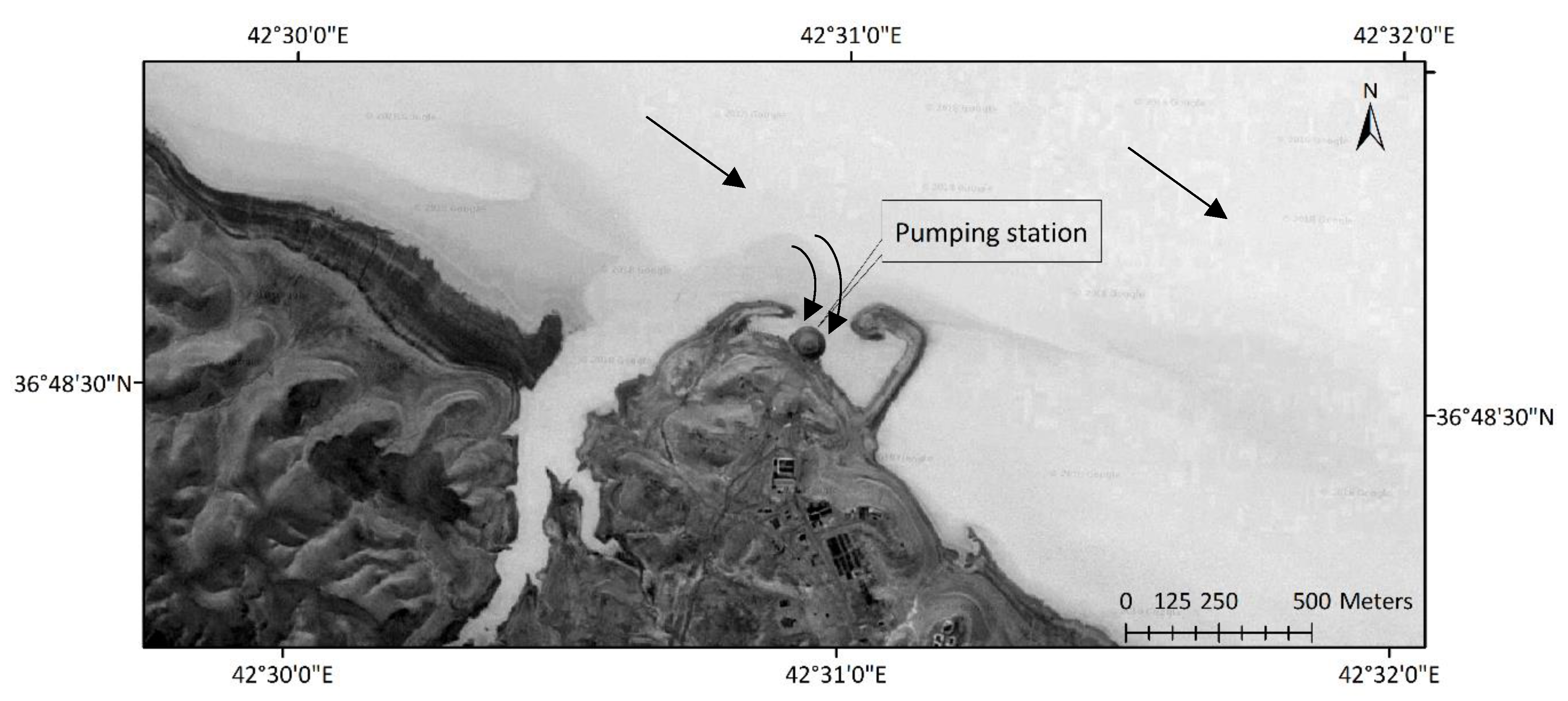
One of the main structures of the Mosul Dam reservoir is the pumping station plant of the North Al-Jazeera irrigation project (Figure 2), which is located on the upper right side of the reservoir, about 46 km upstream of the dam’s axis. The function of the plant is to pump the supplementary irrigation water to the North Al-Jazeera irrigation project, located at a level about 50 m higher than the normal reservoir’s operation level (330 m a.s.l).
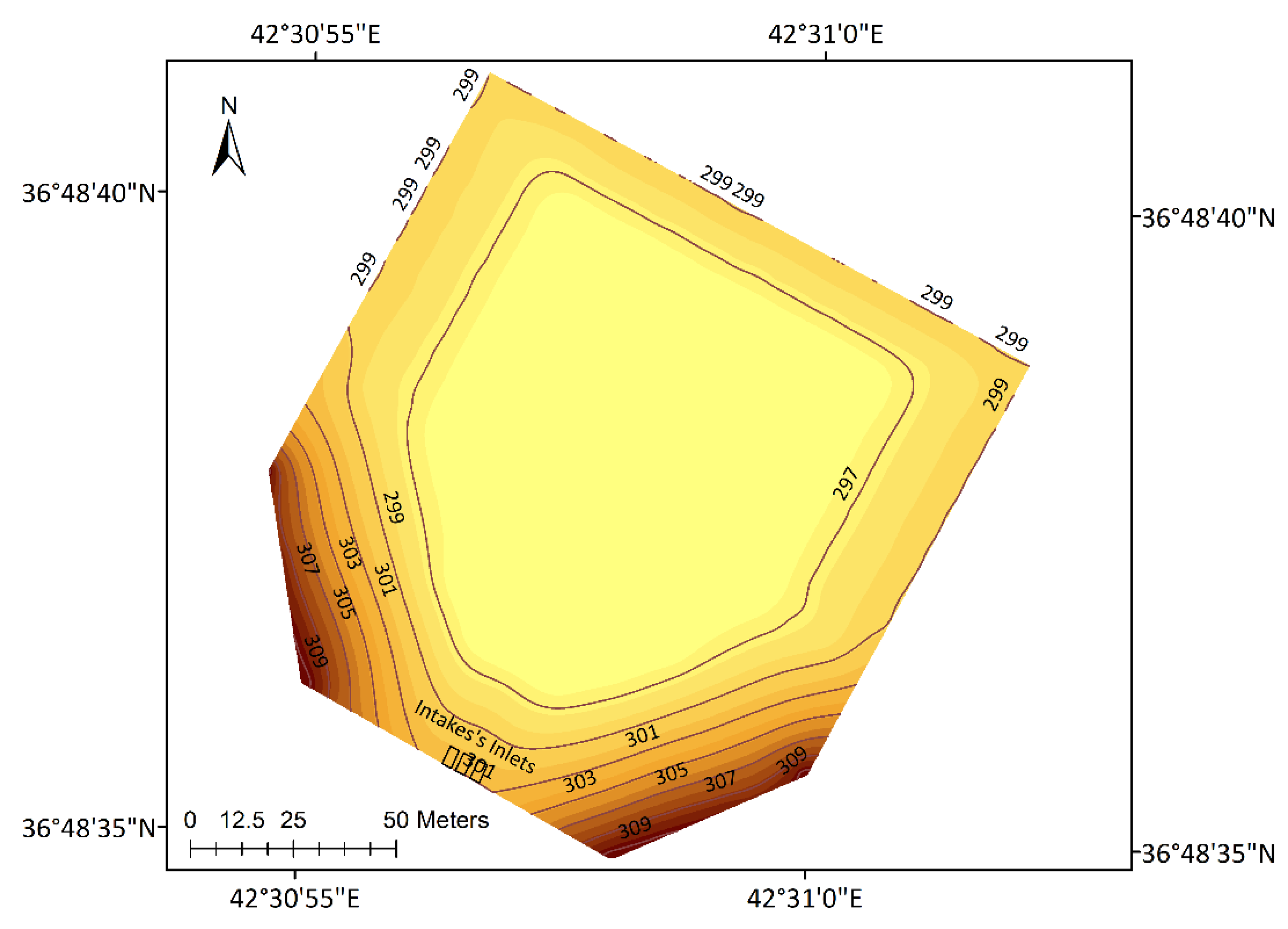
The maximum pumping capacity of the plant is 48 m3/s, and it works between the 5 m head at 305 m a.s.l (minimum reservoir operation level) to 30 m at normal reservoir operation level (330 m a.s.l). The main component of the station is the intake sediment trap; its dimensions about 150 m long and 80 m wide at the base, 100 m wide with sides. The geometry and elevations of the sediment trapping basin is shown in Figure 3. The intake structure consists of three rectangular tunnels of 3 × 3.5 m for each, which changes to a circular section 3.5 m in diameter; the final main part is the central pumping station [21]. This plant suffers from sediment being deposited into the sediment trap basin inside the intake and suction pipes, which leads to a reduction in the pumping rate and plant efficiency. The contribution of the valleys’ flow and withdrawal of flow towards the pumping plant makes the flow regime more complicated, especially near these locations. It is difficult and inefficient to study and analyse such cases using a 1-D model. Only a 2-D or a 3-D model can simulate such cases. To acquire more details on the flow and sediment transport distribution and concentration in all directions along the flow path, a 3-D model was applied in this study.
3. Computational Fluid Dynamics Model
Numerical models for the simulation of flow, sediment transportation, and deposition are considered to be efficient tools with reasonable costs compared to physical models. In reservoir simulation, due to the complexity of flow conditions and hydraulic boundaries, a total 3-D model is essential [13], especially in the studied situation, which is examining the hydraulic structure (intake) and a number of branches that produce secondary flow currents. The sediment simulations in intakes with multiblock option (SSIIM) model was considered in this study. This model depends on computational fluid dynamics (CFD) techniques as a numerical method to solve fluid motion problems. The main advantage of the SSIIM model, compared to the general form of the CFD model, is its ability to simulate sediment transport in a moveable bed with compound geometry, rivers, reservoirs, and surrounding hydraulic structures [26]. This model includes algorithms for different sediment size transport calculations, including, sorting, suspended load, bed load, and bed formation. This model simulates water movement based on a solution of the continuity equation and the Reynolds average Navier–Stokes equation [27]. The following continuity equation is derived from the conservation of mass and momentum:
The Navier–Stokes equation for non-compressible constant density fluid takes the following form:
where is the average velocity in the three directions (i = 1, 2, and 3) in L/T; is the spatial geometric scale (L) in the ith direction; is the density of water (M/L3) is the dynamic pressure (M/L2/T) is the kronecker delta, which is equal to 1 if i equals j and 0 if not; and is the Reynolds stress. The Reynolds stress has been modelled with eddy viscosity and the standard k–ε model in the following form [14]:
where is the turbulent kinetic energy and is the turbulent eddy viscosity.
The change in free water surface elevation is calculated based on solving a partial differential equation of the pressure gradient between the certain cells and neighboring cells.
The sediment load transportation in river flows is usually accomplished in two ways: a suspended load and a bed load. The suspended load represents the fraction of the sediment moved in the suspension when the particle weight is less than the upward turbulent force. Therefore, the load moves higher in the water depth layer than in the bed level. The bed load represents the fraction of sediment moved near or onto the bed by rolling and slipping, which represents the coarse sediment with a weight greater than the upward flow diffusion force. The grain size of the transported sediment, which is greater than 0.062 mm, is considered to be bed load sediment [28].
In the applied model, the sediment load transportation is distributed to a suspended load and bed load. The convection–diffusion equation is then used to compute the sediment load concentration [26]. For the specific suspended sediment size i, the convection–diffusion equation can be written in the following form:
where is the concentration of sediment size i, in volume fraction L3/L3; is the time (T); is the fall velocity of particle size i (L/T); is the coefficient of diffusion; and is the pickup rate of sediment size i, due to erosion.
The considered empirical formula for the sediment concentration near the bed can be estimated based on van Raijn’s formula [29], in the following form:
where is the dimensionless sediment concentration transport of the ith fraction (L3/L3), is the bed shear stress (M/L/T2), is the critical bed shear stress of the sediment particle movement (M/L/T2), is the ith sediment particle diameter (L), is the sediment density (M/L3), and is the kinematic viscosity coefficient (L2/T).
The pickup rate (FR) for a certain particle size i can be defined by the following equation [30]:
where is the concentration of particle size i for the computed time step in the bed cell, and is the fraction of the size of the i bed material (0–1).
4. Data and Model Setup
The input data for the considered model include grid data points for the reservoir geometry and all surrounding valleys as coordinate geometry and elevations. A digital elevation model data point has been set based on the available DEM data [31] (United States Geological Survey, or USGS), as well as an available contour map for the study area before the dam’s construction (1986). Due to the insignificant variation of the main river flow during each month, daily flow data for the Tigris River at the station (upstream of the reservoir) has been considered. In addition to the Tigris River flow, there are ten main valleys around the reservoir considered to be other sources of flow. The soil and water assessment tool model (SWAT) has been applied to estimate the daily surface runoff and sediment loads delivered to the reservoir from the valleys around it [32,33]. The recorded measured sediment load data upstream from the reservoir inlet was considered to create a sediment rating curve [34] to assess the daily sediment loads carried by the river. Furthermore, the assessed sediment load deposited in the reservoir after about 25 years of dam operations, 1.14 km3 [25], was considered for model validation.
Due to the reservoir’s complicated geometry, the studied area is represented by nine blocks for the main reservoir area and the valleys around it, in addition to one nested block focused on the sediment trap basin, as well as an area near the intake of the pumping station to analyse the flow and sediment deposition in more detail for the simulation in this area. The main reservoir was simulated for computational purposes by 100 cells in the streamwise (x) direction, 25 cells in the transversal (y) direction, and a maximum of 10 cells in the vertical direction (z). A total of 2500 cells represent the horizontal layer of the water body, and 10 vertical cells identified the flow depth. As an average, the cell dimensions are 600 × 250 m, in order to save the computational time caused by the huge surface area of the reservoir (375 km2 at the normal water level), and long simulation period (25 years). These large grids can be rationalized due to wide reservoir sections (ranged from 3 to 12 km at the normal operation level), so that there is not big variation in bed level within the considered grid size. Furthermore, a previous study [14] applied the same SSIIM model, and indicated that considering fine cells sizes of the geometry did not give appreciable changes in the results, so the computational time was multiplied. However, for the area of greatest interest neighboring the intake, a nested block was added. The nested block was represented by 45 cells in the streamwise (x) direction, 22 cells in the transversal (y) direction, and a maximum of 10 cells in the vertical direction (z). A total of 990 cells represent the horizontal layer of the area near the intake, and 10 vertical cells were used to identify the flow depth. The grid dimensions are 10 × 10 m, which covers an area of 99 × 103 m2.
The main inflow to the reservoir is from the Tigris River, which during the simulation period (1986–2011) ranged from 3400 m3/s to 90 m3/s. Meanwhile, the reservoir water level ranged between about 332 m a.s.l and 300 m a.s.l. The daily assessment of surface runoff and carried sediment loads were also considered for the different watershed valleys, which were represented as separate blocks connected to the main reservoir. Based on a grain size distribution analysis of samples that were taken from different locations of the study area, previous samples that have been analysed in [35,36]. In addition, the surface soil and runoff sediment load analysis [21], as well as the main river sediment load distribution [37], the range of the considered grain size distribution and fall velocity for all sediment inflow groups is shown in Table 1. The particles’ fall velocities were calculated based on the formula presented by Ponce [38]. The fraction of each size is dependent on the size of the sediment load distribution of the reflected block. As a sample of the fraction of the sediment sizes, the fractions of the measured sediment sizes for the main river flow (Block 1) are shown in Table 1. The empirical formula presented by van Raijn [39] was used to assess the roughness of the reservoir bed based on the size distribution of the bed material’s particles.
5. Model Validation
The model was validated based on the total load deposited in the reservoir from the start of dam operations in 1986 to May 2011. The time for the bathymetry survey was determined in [25], which is the same period of time that was considered for the model simulation. The predicted trapped sediment load in the reservoir for the simulated period was 1.04 km3; this value represents about 9% of the total reservoir storage capacity. Furthermore, the average value of the sediment trap efficiency for the simulated period was about 92%. This simulated trapped sediment (1.04 km3) indicates a good model performance for a long period of simulation compared to measured values (1.14 km3 [25]). The main difference is due to neglecting bed load particles larger than 0.45 mm, which was done to reduce the number of considered particles sizes in the simulation to 11, in order to decrease the simulation’s running time and increase the computational capacity. The considered maximum limit of the particle sizes is based on the maximum particle size carried as bed load and suspended load by the main watercourses around the reservoir, which is 0.4 mm [21], while the median grain size diameter, d50 value of the bed load particles is 12.4 mm [25]. An underestimation of the deposited sediment may also be attributed to an assessment of the sediment inflow of the main flow river based on the created sediment rating curve, as well as the load carried by watercourses around the reservoir; this was assessed based on the simulated values by the SWAT model. The other important variable that was considered for model validation is the suspended load measurement near the intake structure. The second measured values used for model validation were the sediment concentration measurements in [21] at different depths in the reservoir near the intake at two different times, as shown in Table 2. The PBIAS between the measured and simulated sediment concentration was −3.6% (less than ± 10%), indicating very good model performance [41]. Furthermore, the paired t-test value was 0.43 (less than the tabulated value (2) at a 0.05 probability level), indicating that there is no significant difference.
Although 11 sediment grain sizes were considered for the distribution of the sediment load, due to the low flow’s ability to carry and transport large sediment, because of a low average depth flow velocity of 0.0015 m/s to 0.017 m/s near the intake, only the four smallest sizes contributed significantly to the sediment concentration values in this zone of the reservoir.
6. Model Sensitivity to Grid Size and Time Steps
To analyse the uncertainties of the applied numerical model results, sensitivity analysis is one of the most common methods to evaluate the effect of different model parameters. The grid size and time steps are the tested parameters. Due to the large reservoir surface area and long simulation period, the water body in the horizontal direction was represented by coarse grids size (100 × 25 cells, 600 × 250 m as average dimensions). This size could be justified due to wide reservoir’s sections, and there is no significant difference in the bed profile through the considered cells’ dimensions. However, for the most interesting area (neighboring the intake), fine cells are considered (10 m × 10 m) to simulate and obtain more details of different effective factors in this simulation. These considered coarse grids gave reasonable results in comparison with measured values. Then, finer grids were created to test the model’s sensitivity to grids size. The dimensions of the fine grids were half the coarse cells’ size. This makes the number of surface cells multiplied four times (50 × 200 cells), and the computational time was decidedly increased. The fine grid simulation indicated that the difference in the bed profile reaches about 2% in comparison to the considered grids’ size; this insignificant difference corresponds with a previous study [14]. Generally, in large-storage-volume reservoirs, the water level could be considered constant during a relatively short time period (days or a week). Furthermore, the variation of the reservoir’s daily inflow and outflow during most of the years’ time (non-flood period) are relatively minor. For this situation, long time steps could be considered [18], and an hour (3600 s) time step was used. To test the model sensitivity to the time steps, and to check if the selected time step was suitable to the studied situation, different time steps were tested—one double (7200 s) the considered time step, and two smaller time steps (1800 and 900 s). Table 3 shows the percentage of variation of the deposited sediment load for different time steps in the reservoir, compared to a 3600 s time step as a reference time.
The maximum variation for different time steps was about 6%. The main reason for this limited deviation is that the long period simulation excludes the effect of different variations, which usually happens for short periods [42], and the daily values of inflow, outflow, and storage level made the simulation stable throughout the applied time steps.
7. Results and Discussion
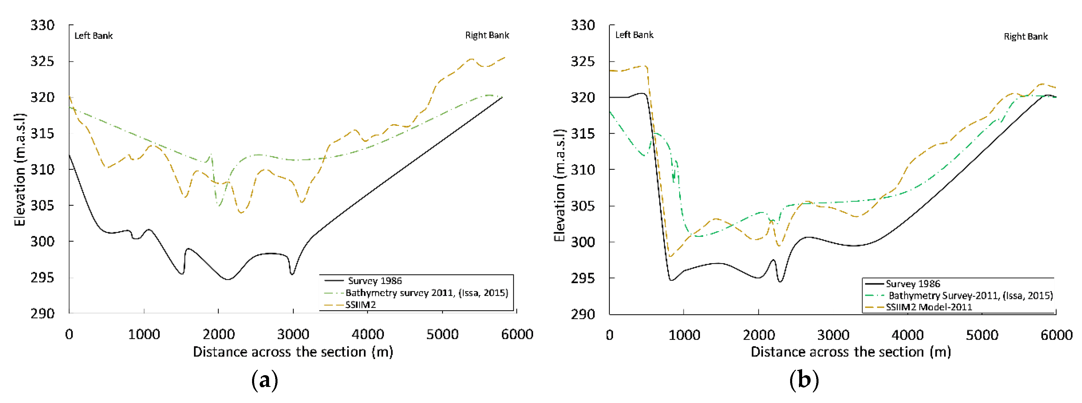
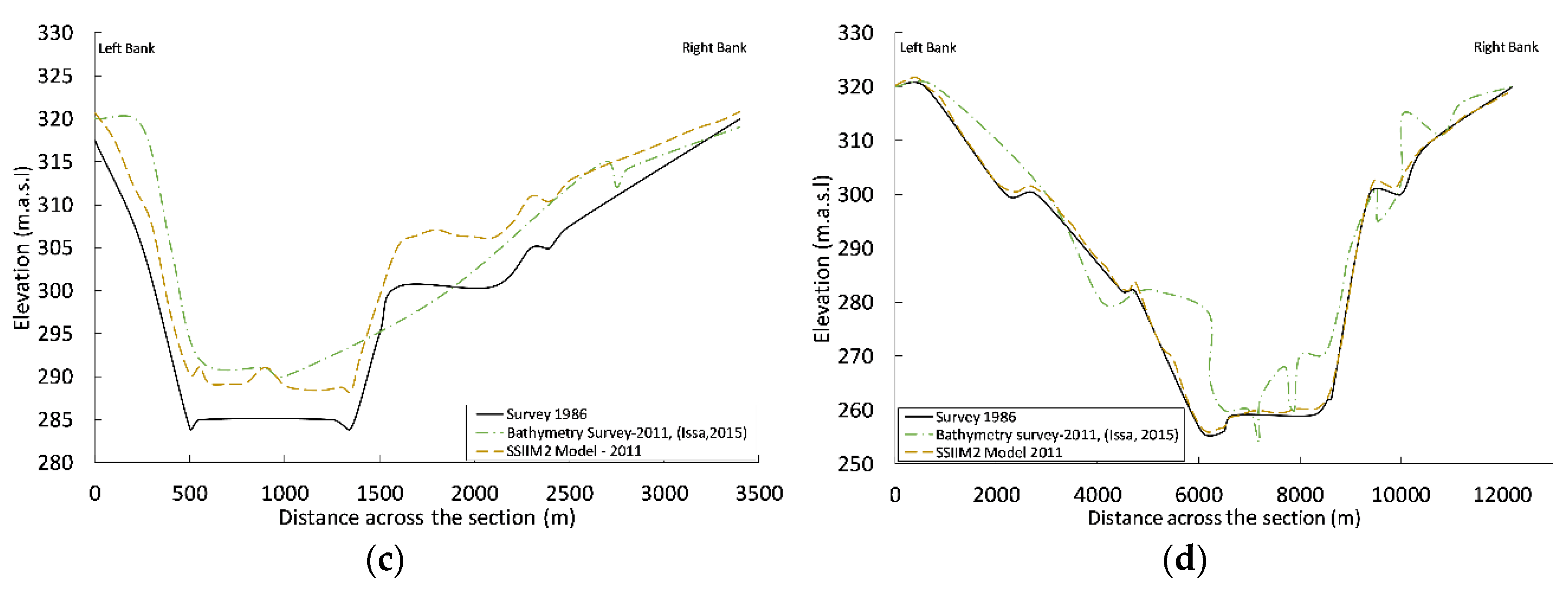
After 25 years of flow, sediment transport, deposition, and erosion simulations (from July 1986 to May 2011), the result of the reservoir bed formation was compared with the bathymetry survey done in May 2011 [25]. To evaluate the model’s performance, four sections along the reservoir were compared. Figure 4a–d shows the original reservoir’s bed level before dam operations (1986), the results of the bathymetry survey [25], and the results of the SSIIM2 model simulation, respectively. The sections are selected as follows: (1) the upper third of the reservoir, (2) near the pumping station, (3) downstream from the pumping station, and (4) upstream from the dam axis. The locations of sections 1, 2, 3, and 4 are at a distance of about 55.5 km, 51.00 km, 42.0 km, and 6.5 km upstream the dam axis, respectively.
In the first upper section (Figure 4a), the average settled sediment depths across the section based on the bathymetry survey and simulated values are about 10.5 m and 9.7 m, respectively, in comparison with the original bad levels before dam operations. This difference represents about 7.6% of the measured value, which is attributed to neglecting the coarse sediments in simulation. Usually, coarse sediments are deposited in the upper part of the reservoirs when the velocity is reduced, gradually leading to a reduction in the sediment transport capacity of the flow. For the second considered section (Figure 4b), the average settled sediment across the section reached about 4.9 m and 4.7 m at the end of simulation for the bathymetry survey and simulation, respectively. Although the difference between them is not more than 4%, the main difference is the distribution of the deposited sediment near the left bank. It can be noted that the bathymetry survey shows a slope side slip near this bank, due to the relatively sharp side slope of 8.3%. The main difference between the measured and simulated bed formation may be due to the slope stability of the reservoir banks, which is not considered in the simulation model. In the third section (Figure 4c), the accumulated average settled sediments across the sections are 4.5 m and 4.4 m for the bathymetry survey and the simulated value, respectively. Furthermore, the differences in sediment deposition formation are mostly within 1000 m to 1800 m from the left bank, due to bank’s side slip and soil accumulation near the section bed. The final considered section is shown in Figure 4d, at a distance of about 6500 m upstream from the dam axis. It is apparent in the figure that the distribution of the deposited sediment is non-uniform with the flow path and sediment load concentration distribution. This non-uniformity is mainly attributed to the instability of the bank’s slope, which leads to an accumulation of the slip soil near the relatively flat part of the section, as shown in Figure 4b–d. The average accumulation of the sediment across this section is 5.4 m for the bathymetry survey, while the simulated value is only about 1.1 m. This average measured sediment deposition depth is unusual in this section; typically, the average sediment deposition that is reduced with the flow distance in storage reservoirs is attributed to a reduction of the sediment concentration, with a flow velocity reduction along the flow path.
Due to this local soil slip, which is not considered in the model, the sediment deposited depth was higher than expected. This relatively high deposition depth in the reservoir sections near the dam axis suggests that this change in bed formation is due to the side bank’s slip, and not just sediment deposition. This analysis may corroborate previous studies [43,44], which mentioned that about 3500 m3 of the left bank soil of the Mosul Dam Reservoir were eroded during the flood wave of 1988, and that the right bank river section is characterized by a steep slope. The values of the considered statistical criteria (percent bias and t-test) are used to evaluate the deposited sediment depths in the selected sections, as shown in Table 4.
For the first upper three sections, the PBIAS values were less than ±10%, indicating very good model performance [41], and the t-test values were less than the tabulated values (2.0 at a 0.05 probability level), indicating that the differences of the sediment depths between the observed and simulated values are insignificant. For the fourth section, the PBIAS value was greater than 10%, meaning that the model performance is unsatisfactory. The t-test value was 2.1 (greater than the tabulated value), meaning that the differences are significant between the measured and simulated sediment depths in this section. Generally, the model performance for assessment of sediment detachment, transportation, and deposition can be considered reasonable in comparison with measured values, but the main differences are due to slope side slips, which are expected to have happened in some locations; this soil movement is not being considered in the model. In applications of the numerical models, commonly there are a number of uncertainties related to input data, exact geometry simulation, and approximation in the numerical solution; the reaching of full convergence, in addition to another errors, makes the application of such models need validation to reflect and apply their results confidently.
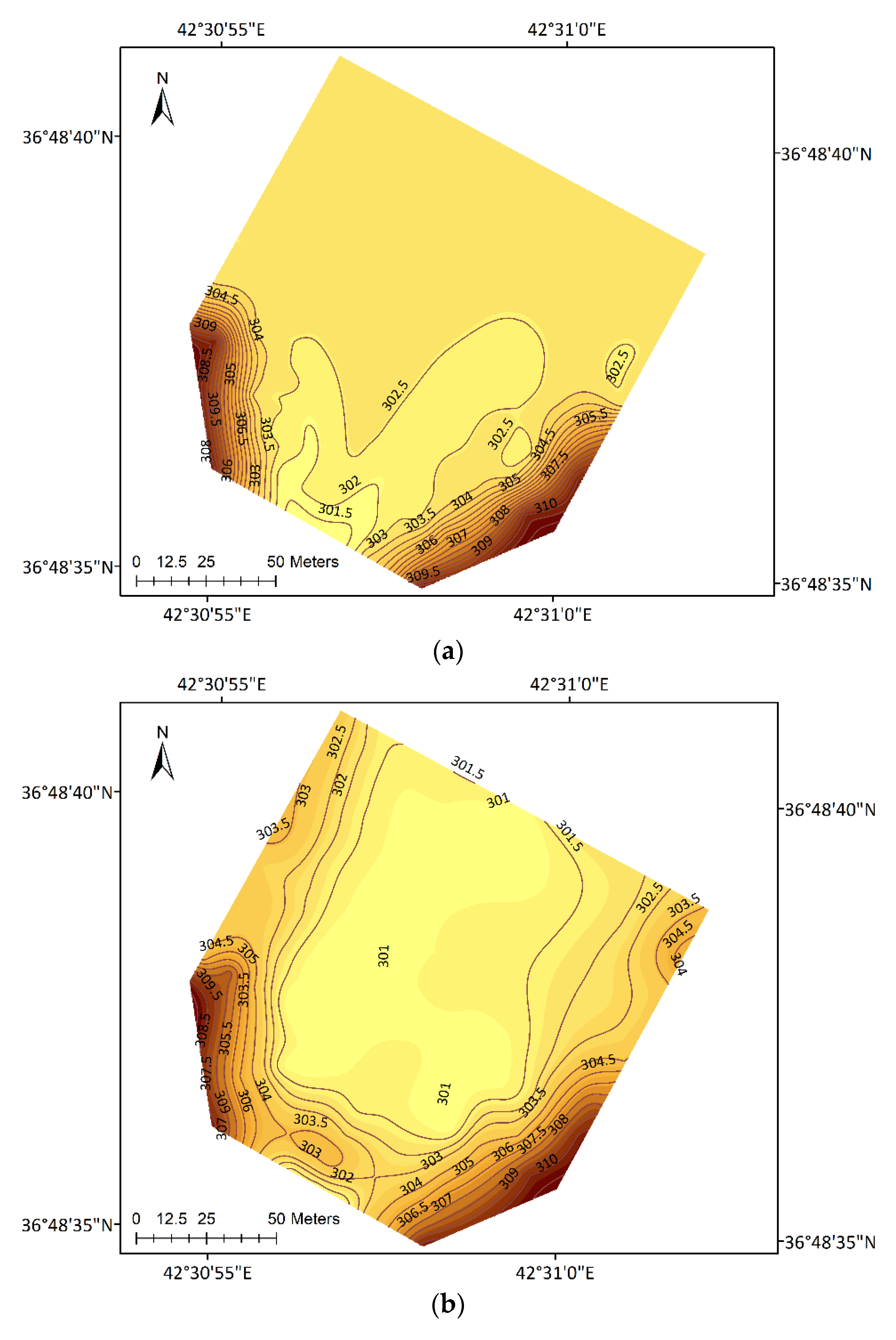
This study also aims to focus on the area near the intake of the pumping station, where there is a sediment trapping basin in front of the studied pumping station’s intake that suffers from sediment accumulation, leading to a reduction in pumping efficiency. The sediment load concentrations at the selected point in front of the intake were considered for model validation, while the depths of the measured deposited sediment [21] were compared with the simulated values by the SSIIM2 model. Figure 3 shows the geometry of the sediment trapping basin at the beginning of the dam operation in 1986, while Figure 5a shows the measured basin level in February 2001, and Figure 5b shows the simulated values in February 2001.
The measured deposited sediment depth at the inlet of the basin ranged between 3.4 m and 4.4 m [21], while the average value for the considered area surrounding the basin (21,540 m2) (Figure 5a) was 5.2 m. In comparison with the simulated values, the sediment depth deposition at the intake ranged from 3.1 m to 4.9 m, while the average value for the whole the area was 4.5 m. The sediment depth measurements at different points in the trapping basin were compared with the simulated values. The results indicate that the PBIAS between the measured and observed values is 3.6% (less than 10%), while the t-test value is 1.41, less than the critical tabulated values at a 0.05 probability level. This indicates that there is no significant difference between the observed and simulated values. The deposited sediment volume in the considered area, shown in Figure 5a,b, are 0.111 × 10⁶ m3 and 0.096 × 10⁶ m3 for the observed and simulated values, respectively.
8. Conclusions
The computational fluid dynamics model SSIIM2 was applied in this study to simulate flow, sediment transport, and deposition in a storage reservoir subject to water withdraw via a pumping station. The considered 3-D model (SSIIM2) solves the Reynolds average Navier–Stokes equation to simulate the flow and the convection–diffusion equation with van Raijn’s formula, which simulates sediment concentration and variations in bed formation. The total deposited sediment load after 25 years of dam operation and sediment concentration at nine points near the intake were considered for model validation. The model sensitivity to grid size and time steps were tested, and the variation in sediment deposited in the reservoir due to duplicate horizontal grids number was not substantial. It did not exceed 2%. The minor variation in bed level through the fine and coarse grid sizes might have reduced the variation in simulation results of this study. However, more accurate topography data possibly gives different results for the effects of grid size. Furthermore, the maximum difference in deposited sediment loads reached about 6% for different tested time steps. The reduction in time steps leads to more accurate simulation, but requires long computational time. The deposited sediment thicknesses across the reservoir sections were compared with measured values (bathymetry survey [25]). Furthermore, the simulated sediment deposition depths in the trapping basins of the intake were compared with the measured values [21]. The selected statistical criteria PBIAS and t-tests indicate that the model’s performance for sediment deposition distribution in the reservoir is reasonable. The high sediment depth difference between the simulated and measured values in some sections can be attributed to the accumulation of slip banks in some locations, which is not simulated in this model. This can be considered a model weakness, as it may perform less well in some locations, especially when the banks’ slopes are steep. For the trapping basin of the pumping station, the compared values between measured and simulated sediment depth at the different points result in values of 3.58% and 1.14 for PBIAS and the t-test, respectively, indicating that the model performance is satisfactory. The results indicate that the finest sediment particles sizes between 0.002 mm and 0.012 mm have a significant negative effect on sediment deposition near the intake and on pumping station operational efficiency.
Author Contributions
M.E.M. did the conceptualization, methodology, software, validation, formal analysis, investigation, methodology, data curation, visualization, writing—original draft preparation, and writing—review and editing. N.A.-A., S.K., and J.L. did the validation, visualization, project administration, supervision, and writing—review and editing. All authors have read and agreed to the published version of the manuscript.
Funding
This research received no external funding.
Acknowledgments
The authors would like to thank Issa Elias Issa for supplying the bathymetry survey data for the Mosul Dam reservoir sections done in 2011, as well as Florian Thiery at Luleå University of Technology for allowing us to use his work station computer to run the fine grid and small time step simulations.
Conflicts of Interest
The authors declare no conflict of interest.
References
- George, M.W.; Hotchkiss, R.H.; Huffaker, R. Reservoir sustainability and sediment management. J. Water Resour. Plan. Manag. 2017, 143, 04016077. [Google Scholar] [CrossRef] [Green Version]
- Cerda, A.; Keesstra, S.; Rodrigo-Comino, J.; Novara, A.; Pereira, P.; Brevik, E.C.; Giménez-Morera, A.; Fernandez-Raga, M.; Fernández, M.P.; Di Prima, S.; et al. Runoff initiation, soil detachment and connectivity are enhanced as a consequence of vineyards plantations. Environ. Manag. 2017, 202, 268–275. [Google Scholar] [CrossRef] [PubMed] [Green Version]
- Keesstra, S.D.; Rodrigo-Comino, J.; Novara, A.; Giménez-Morera, A.; Pulido, M. Catena Straw mulch as a sustainable solution to decrease runo ff and erosion in glyphosate-treated clementine plantations in Eastern Spain. An assessment using rainfall simulation experiments. Catena 2019, 174, 95–103. [Google Scholar] [CrossRef]
- Cerdà, A.; Rodrigo-Comino, J.; Giménez-Morera, A.; Keesstra, S.D. An economic, perception and biophysical approach to the use of oat straw as mulch in Mediterranean rainfed agriculture land. Ecol. Eng. 2017, 108, 162–171. [Google Scholar] [CrossRef] [Green Version]
- Keesstra, S.D.; Dam, O.V.; Verstraeten, G.; van Huissteden, J. Catena Changing sediment dynamics due to natural reforestation in the Dragonja catchment, SW Slovenia. Catena 2009, 78, 60–71. [Google Scholar] [CrossRef]
- Cerdà, A.; Rodrigo-Comino, J.; Giménez-Morera, A.; Novara, A.; Pulido, M. Policies can help to apply successful strategies to control soil and water losses. The case of chipped pruned branches (CPB ) in Mediterranean citrus plantations Land Use Policy Policies can help to apply successful strategies to control soil and water. Land Use Policy 2018, 75, 734–745. [Google Scholar] [CrossRef] [Green Version]
- Leo, H. Technical Workshop TW 5 Physical and Numerical Modelling—Role and Limits Programme; ICOLD CIGB: Prague, Czechia, 2017; pp. 5–8. [Google Scholar]
- Hedlund, A. Evaluation of RANS Turbulence Models for the Simulation of Channel Flow; Technical Report; Uppsala Universitet, Department of Engineering Sciences: Uppsala, Sweden, 2014. [Google Scholar]
- Morris, G.; Jiahua, F. Reservoir Sedimentation Handbook: Design and Management of Dams, Reservoirs and Watersheds for Sustainable Use; McGraw-Hill: New York, NY, USA, 1998. [Google Scholar]
- Esmaeili, T.; Sumi, T.; Kantoush, S.A.; Kubota, Y.; Haun, S. Three-dimensional numerical modeling of sediment flushing: Case study of Dashidaira Reservoir, Japan. In Proceedings of the 36th IAHR World Congress, The Hague, The Netherlands, 28 June–3 July 2015. [Google Scholar]
- Faghihirad, S.; Lin, B.; Falconer, R.A. Application of a 3D layer integrated numerical model of flow and sediment transport processes to a reservoir. Water 2015, 7, 5239–5257. [Google Scholar] [CrossRef] [Green Version]
- Zhang, Q.; Hillebrand, G.; Moser, H.; Hinkelmann, R. Simulation of non-uniform sediment transport in a German Reservoir with the SSIIM Model and sensitivity analysis. In Proceedings of the 36th IAHR Wolrd Congress, The Hague, The Netherlands, 28 June–3 July 2015. [Google Scholar]
- Haun, S.; Kjærås, H.; Løvfall, S.; Olsen, N.R.B. Three-dimensional measurements and numerical modelling of suspended sediments in a hydropower reservoir. J. Hydrol. 2013, 479, 180–188. [Google Scholar] [CrossRef]
- Agrawal, A.K. Numerical Modelling of Sediment Flow in Tala Desilting Chamber. Master’s Thesis, Norwegian University of Science and Technology, Trondheim, Norway, 2005. [Google Scholar]
- Hoven, L.E. Three-Dimensional Numerical Modelling of Sediments in Water Reservoirs. Master’s Thesis, Norwegian University of Science and Technology, Trondheim, Norway, 2010. [Google Scholar]
- Haun, S.; Olsen, N.R.B. Three-dimensional numerical modelling of the flushing process of the Kali Gandaki hydropower reservoir. Lakes Reserv. Res. Manag. 2012, 17, 25–33. [Google Scholar] [CrossRef]
- Esmaeili, T.; Sumi, T.; Kantoush, S.A.; Kubota, Y.; Haun, S.; Rüther, N. Three-dimensional numerical study of free-flow sediment flushing to increase the flushing efficiency: A case-study reservoir in Japan. Water 2017, 9, 900. [Google Scholar] [CrossRef] [Green Version]
- Olsen, N.R.B.; Hillebrand, G. Long-time 3D CFD modeling of sedimentation with dredging in a hydropower reservoir. J. Soils Sediments 2018, 18, 3031–3040. [Google Scholar] [CrossRef]
- Hämmerling, M.; Walczak, N.; Nowak, A.; Mazur, R.; Chmist, J. Modelling velocity distributions and river bed changes using computer code SSIIM below sills stabilizing the riverbed. Pol. J. Environ. Stud. 2019, 28, 1165–1179. [Google Scholar] [CrossRef]
- Keesstra, S.; Pedro, J.; Saco, P.; Parsons, T.; Poeppl, R. The way forward: Can connectivity be useful to design better measuring and modelling schemes for water and sediment dynamics? Science of the Total Environment The way forward: Can connectivity be useful to design better measuring and modelling schemes. Sci. Total Environ. 2018, 644, 1557–1572. [Google Scholar] [CrossRef] [PubMed]
- Abdul Baqi, Y.T. Evaluation of Sediment Accumulation at the Intakes of the Main Pumping Station of North Jazira Irrigation Project. Master’s Thesis, Mosul University, Mosul, Iraq, 2001. [Google Scholar]
- Bi, S.; Zhang, Y.; Han, N.; Long, X. Numerical simulation on the flow field of inlet structure of dongsong pumping station. In Advances in Water Resources and Hydraulic Engineering—Proceedings of 16th IAHR-APD Congress and 3rd Symposium of IAHR-ISHS; Springer: Berlin/Heidelberg, Germany, 2009; pp. 1731–1736. [Google Scholar]
- Gabl, R.; Gems, B.; Birkner, F.; Hofer, B.; Aufleger, M. Adaptation of an existing intake structure caused by increased sediment level. Water 2018, 10, 1066. [Google Scholar] [CrossRef] [Green Version]
- Charafi, M.M. Two-dimensional numerical modeling of sediment transport in a dam reservoir to analyze the feasibility of a water intake. Int. J. Mod. Phys. C 2019. [Google Scholar] [CrossRef]
- Issa, E.I. Sedimentological and Hydrological Investigation of Mosul Dam Reservoir Issa Elias Issa. Ph.D. Thesis, Luleå University of Technology, Luleå, Sweden, 2015. [Google Scholar]
- Olsen, N.R.B. A Three-Dimensional Numerical Model for Intakes with Multiblock Option SSIIM, User’s Manual; Department of Civil and Environmental Engineering, Norwegian University of Science and Technology: Trondheim, Norway, 2018. [Google Scholar]
- Olsen, N.R.B. SSIIM—A Three-dimensional numerical model for simulation of water and sediment flow N.R.B. Environment 1993, 2, 14328–14336. [Google Scholar]
- Hickin, E.J. Sediment transport. In River Geomorphology; Hickin, E.J., Ed.; John Wiley and Sons: New York, NY, USA, 1995; pp. 71–107. [Google Scholar]
- van Rijn, L.C. Sediment transport, Part I: Bed load transport. J. Hydraul. Eng. ASCE 1984, 110, 1431–1456. [Google Scholar] [CrossRef] [Green Version]
- Hillebrand, G.; Klassen, I.; Olsen, N.R.B. 3D CFD modelling of velocities and sediment transport in the Iffezheim hydropower reservoir. Hydrol. Res. 2016, 48, 147–159. [Google Scholar] [CrossRef]
- Center for Earth Resources Observation and Science, USGS Kilauea Team Finalist for the ‘Oscars’ of Government Service. Available online: https://earthexplorer.usgs.gov/ (accessed on 26 March 2018).
- Mohammad, M.E.-A.; Al-Ansari, N.; Knutsson, S. Runoff and sediment load from the right bank valleys of Mosul Dam reservoir. J. Civ. Eng. Archit. 2012, 6, 1414–1419. [Google Scholar]
- Mohammad, M.E.-A.; Al-Ansari, N.; Knutsson, S. Application of Swat Model to estimate the sediment load from the left bank of Mosul Dam. J. Adv. Sci. Eng. Res. 2013, 3, 47–61. [Google Scholar]
- Mohammad, M.E.; Al-Ansari, N.; Issa, I.E.; Knutsson, S. Sediment in Mosul Dam reservoir using the HEC-RAS model. Lakes Reserv. Res. Manag. 2016, 21, 235–244. [Google Scholar] [CrossRef] [Green Version]
- Al-Sinjari, M.A.F. Characterization and Classification of Some Vertisols West of Duhok Governorate. Ph.D. Thesis, Soil and Water science Department, Mosul University, Mosul, Iraq, 2007. [Google Scholar]
- Alsayegh, A.M. Using Remote Sensing Data to Evaluate Land Use for Some Soil Properties South West Mosul Dam Reservoir. Master’ Thesis, Mosul University, Mosul, Iraq, 2006. [Google Scholar]
- Kurukji, E.M. Sediment Characteristics of River Tigris between Zakho and Fatha. Master’ Thesis, University of Mosul, Mosul, Iraq, 1985. [Google Scholar]
- Ponce, V.M. Engineering hydrology, principles and practices. In Engineering Hydrology, Principles and Practices; Prentice Hall: Upper New Jersey River, NJ, USA, 1989; pp. 534–535. [Google Scholar]
- van Rijn, L.C. Sediment transport, part III: Bed forms and alluvial roughness. J. Hydraul. Eng. 1984, 110, 1733–1754. [Google Scholar] [CrossRef]
- Al-Naqib, S.Q.; Al-Taiee, T.M. The Effect of Suspended Sediment Load Transported by Fayda and Baqaq Wadies on Mosul Lake as Related to Watershed Characteristics, Confidential Paper Mosul; Mosul University: Mosul, Iraq, 1990. [Google Scholar]
- Pérez-Sánchez, J.; Senent-Aparicio, J.; Segura-Méndez, F.; Pulido-Velazquez, D.; Raghavan, S. Evaluating hydrological models for deriving water resources in peninsular Spain. Sustainability 2019, 11, 2872. [Google Scholar] [CrossRef] [Green Version]
- Zhang, Q.; Hillebrand, G.; Hoffmann, T.O.; Hinkelmann, R. Estimating long-term evolution of fine sediment budget in the Iffezheim reservoir using a simplified method based on classification of boundary conditions Estimating long-term evolution of fine sediment budget in the Iffezheim reservoir using a simplified. Geophys. Res. Abstr. 2017, 19, EGU2017–9039. [Google Scholar]
- Al-Taiee, T.M.; Al-Naqub, S.Q.; Al-Kawaz, M.A. Study of the Sediment in the Regulating Dam Lake, Source, Amounts and Solution; Water Resources Research Center, Mosul University: Mosul, Iraq, 1990. [Google Scholar]
- Al-Ansari, N.; Rimawi, O. The influence of the Mosul Dam on the bed sediments and morphology of the River Tigris. In Proceedings of the Human Impact on Erosion and Sedimentation (Proceedings of International Symposium), Rabat, Morocco, 1997; pp. 291–300. [Google Scholar]
Figure 1.
The topography (Digital Elevation Model (DEM)) of the Mosul Dam reservoir surrounded by the main valleys.
Figure 1.
The topography (Digital Elevation Model (DEM)) of the Mosul Dam reservoir surrounded by the main valleys.

Figure 2.
A satellite image (Google image) of the pumping station.

Figure 3.
Geometry and elevations of the simulated sediment trap basin of the Mosul Dam pumping station in 1986.
Figure 3.
Geometry and elevations of the simulated sediment trap basin of the Mosul Dam pumping station in 1986.

Figure 4.
Measured and simulated bed levels for the four selected sections, as follows: (a) section 1, (b) section 2, (c) section 3, and (d) section 4.
Figure 4.
Measured and simulated bed levels for the four selected sections, as follows: (a) section 1, (b) section 2, (c) section 3, and (d) section 4.


Figure 5.
(a) Measured sediment elevations in the sediment trap basin in February 2001 (based on measured values [21]); (b) Simulated sediment elevations in the sediment trap basin in February 2001 (sediment simulations in intakes with multiblock option (SSIIM2)).
Figure 5.
(a) Measured sediment elevations in the sediment trap basin in February 2001 (based on measured values [21]); (b) Simulated sediment elevations in the sediment trap basin in February 2001 (sediment simulations in intakes with multiblock option (SSIIM2)).


Table 1.
The considered sediment size range, fall velocity, and fractions of the main river.
| No. | Particle Size (mm) | Fall Velocity (mm/s) | Fraction (%) |
|---|---|---|---|
| 1 | 0.425 | 56.28 | 4.8 |
| 2 | 0.15 | 13.46 | 2.0 |
| 3 | 0.075 | 4.44 | 1.3 |
| 4 | 0.057 | 2.56 | 2.1 |
| 5 | 0.042 | 1.39 | 3.4 |
| 6 | 0.029 | 0.67 | 5.1 |
| 7 | 0.017 | 0.23 | 8.0 |
| 8 | 0.012 | 0.12 | 5.7 |
| 9 | 0.008 | 0.06 | 6.9 |
| 10 | 0.005 | 0.03 | 24.7 |
| 11 | 0.002 | 0.01 | 36.0 |
Table 2.
Measured and simulated sediment concentration at different points in the front of the intake.
Table 2.
Measured and simulated sediment concentration at different points in the front of the intake.
| Point No. | Location | Date | Simulated Sediment Concentration (g/m3) for Different Particles Sizes | Total Simulated Conc. (g/m3) | * Measured Conc. (g/m3) | |||
|---|---|---|---|---|---|---|---|---|
| 0.002 (mm) | 0.005 (mm) | 0.008 (mm) | 0.012 (mm) | |||||
| 1 | In front of the intake (surface) | 8 February 2001 | 12.00 | 0.32 | 0.012 | 0.0007 | 12.4 | 9.5 |
| 2 | In front of the intake (2 m above the bed) | 8 February 2001 | 14.70 | 0.58 | 0.037 | 0.0024 | 15.4 | 17.0 |
| 3 | In front of the intake (near the bed) | 18 February 2001 | 17.30 | 0.92 | 0.078 | 0.0045 | 18.3 | 19.0 |
| 4 | In front of the intake (2 m above the bed) | 18 February 2001 | 16.80 | 0.86 | 0.071 | 0.0040 | 17.8 | 13.0 |
| 5 | In front of the intake (2 m below water surface) | 18 February 2001 | 15.20 | 0.64 | 0.043 | 0.0017 | 15.9 | 19.0 |
| 6 | In left side of the intake (2 m above the bed) | 18 February 2001 | 15.40 | 0.68 | 0.048 | 0.0021 | 16.2 | 19.0 |
| 7 | At 50 m front of the intake (2 m above the bed) | 18 February 2001 | 15.30 | 0.66 | 0.045 | 0.0020 | 16.0 | 20.0 |
| 8 | At 100 m front of the intake (2 m above the bed) | 18 February 2001 | 15.00 | 0.62 | 0.040 | 0.0015 | 15.6 | 9.0 |
| 9 | At 150 m front of the intake (2 m above the bed) | 18 February 2001 | 15.20 | 0.64 | 0.043 | 0.0018 | 15.9 | 13.0 |
* [21].
Table 3.
Percent of deposited sediment load variation for different time steps.
| Time Steps (s) | 7200 | 3600 | 1800 | 900 |
|---|---|---|---|---|
| Deposited sediment changes (%) | −0.7 | - | 3.4 | 5.9 |
Table 4.
Measured and simulated sediment thickness at the four selected sections and the considered statistical criteria.
Table 4.
Measured and simulated sediment thickness at the four selected sections and the considered statistical criteria.
| Section No. | Section Location Upstream of the Dam Axis (km) | Average Measured Sediment Thickness (m) | Simulated Sediment Depth (m) | Percent Bias (PBIAS, %) | t-Test Value |
|---|---|---|---|---|---|
| 1 | 55.5 | 10.5 | 9.7 | 6.5 | 1.41 |
| 2 | 51.0 | 4.9 | 4.7 | 4.8 | 0.38 |
| 3 | 42.0 | 4.5 | 4.4 | −9.1 | 0.56 |
| 4 | 6.5 | 5.4 | 1.1 | 80.7 | 2.11 |
© 2020 by the authors. Licensee MDPI, Basel, Switzerland. This article is an open access article distributed under the terms and conditions of the Creative Commons Attribution (CC BY) license (http://creativecommons.org/licenses/by/4.0/).
Share and Cite
MDPI and ACS Style
Mohammad, M.E.; Al-Ansari, N.; Knutsson, S.; Laue, J. A Computational Fluid Dynamics Simulation Model of Sediment Deposition in a Storage Reservoir Subject to Water Withdrawal. Water 2020, 12, 959. https://doi.org/10.3390/w12040959
AMA Style
Mohammad ME, Al-Ansari N, Knutsson S, Laue J. A Computational Fluid Dynamics Simulation Model of Sediment Deposition in a Storage Reservoir Subject to Water Withdrawal. Water. 2020; 12(4):959. https://doi.org/10.3390/w12040959
Chicago/Turabian StyleMohammad, Mohammad E., Nadhir Al-Ansari, Sven Knutsson, and Jan Laue. 2020. "A Computational Fluid Dynamics Simulation Model of Sediment Deposition in a Storage Reservoir Subject to Water Withdrawal" Water 12, no. 4: 959. https://doi.org/10.3390/w12040959
Note that from the first issue of 2016, this journal uses article numbers instead of page numbers. See further details here.