Levee Breaching: A New Extension to the LISFLOOD-FP Model

Abstract

Levee failures due to floods often cause considerable economic damage and life losses in inundated dike-protected areas, and significantly change flood hazard upstream and downstream the breach location during the event. We present a new extension for the LISFLOOD-FP hydrodynamic model which allows levee breaching along embankments in fully two-dimensional (2D) mode. Our extension allows for breach simulations in 2D structured grid hydrodynamic models at different scales and for different hydraulic loads in a computationally efficient manner. A series of tests performed on synthetic and historic events of different scale and magnitude show that the breaching module is numerically stable and reliable. We simulated breaches on synthetic terrain using unsteady flow as an upstream boundary condition and compared the outcomes with an identical setup of a full-momentum 2D solver. The synthetic tests showed that differences in the maximum flow through the breach between the two models were less than 1%, while for a small-scale flood event on the Secchia River (Italy), it was underestimated by 7% compared to a reference study. A large scale extreme event simulation on the Po River (Italy) resulted in 83% accuracy (critical success index).

1. Introduction

Flood risk management is a crucial yet challenging task. In 2018, floods caused 19.7 billion US$ in economic losses worldwide [1]. According to [2], global warming under different socio-economic scenarios would lead to increasing flood risk in Europe. Moreover, ref. [2] clearly points out that, without further adaptation, flood defense structures will be breached more frequently in the future. Therefore, the development of new strategies for flood risk reduction is crucial. As a primary element in this, flood hazard modelling encompasses reproduction of the hydraulic behaviour of flood water and its interaction with topographical features and engineering structures in the floodplain. Such structures may partially or entirely control the flood dynamics, which is especially evident in heavily modified terrain with complex networks of levees and embankments. Therefore, it is important to identify flooding patterns in case of possible levee breaches for both low- and high-intensity events.

Levee breaches may occur due to different mechanisms such as overtopping, geohydraulic failure or piping, and local and global static failure [3,4]. Such failures involve a complex pattern of possible consequences for river systems [5,6]. Protected floodplains remain vulnerable in case of embankment breaches, which is often termed the residual risk [7,8]. For instance, multiple levee failures in the Greater New Orleans area in 2005 following the passage of hurricane Katrina resulted in the deaths of over 1100 people and caused enormous economic damage, flooding 80% of the city [9]. Another example is the 1993 Mississippi flood, when the levees breached at numerous locations along a rather large reach of the river causing 32 deaths and $15 billion in economic damage [10]. Alongside record events in terms of their magnitude, floods with much lower recurrence interval may cause significant losses. For instance, a five-year return period flood on the Secchia River (Northern Italy) in 2014 turned into a disaster when the levee breached due to burrowing animals causing €400 million in monetary damages [11]. Together with severe damage, human losses, and infrastructure disruptions due to sudden lowering of the embankment crests, levee breaches may reduce hydraulic loads upstream and downstream, and hence affect inundation patterns and the probability of failure elsewhere in the river system [5,12].

Despite the obvious adverse effects of levee failures, there are other additional strategic aspects to consider. One flood management strategy is controlled flooding (activation of off-line floodplain storage) [13]. Therefore, it is important to have an understanding of how floods behave on a basin scale and which floodplains it is sensible to activate in a given flood scenario. For this, it is important to jointly assess levee breach effects, both adverse and beneficial. Due to system effects, for large river basins, such assessments have to be performed on geographically large areas and cannot be adequately captured by local, albeit very detailed, studies [14].

There are numerous tools that offer a levee breach component to simulate floods (e.g., HEC-RAS, Delft3D, EMBANK, RFSM, MIKE 11 and 21, Tuflow, TELEMAC2D, Sobek, HR BREACH, BASEMENT, 2DEF, PARFLOOD to name a few, see, e.g., [15,16,17,18]. They allow for simulation of the breach with a high level of detail and consider the breach evolution and forcing conditions in order to compute changes in the breach width and consequent flow entering the floodplain. Some associated uncertainties are flow conditions, geotechnical embankment properties and variability of external forces [17,18]. Moreover, other limitations related to the usage of those models, such as data availability, set up time and computational costs, pose a significant constraint. This especially becomes a critical burden when generating the levee breaching scenarios for large-scale studies. There have been studies done to review already existing modelling techniques and tools [16,19,20,21,22,23]. Based on those studies, the models can be divided into three large groups, namely empirical, semi-physically, and fully physically based codes [19]. Empirical models solely rely on the post-event surveys and model parameterisation is based on predictor equations, which are in turn derived to best fit the model. Semi-physically based models (also called analytical or parametric models) use physical equations, but with some assumptions in order to reduce computation time and expand applicability. Finally, physically based models account for flow regime, breach evolution over time and space and associated parameters [16,19]. They form a large group, since most of above-mentioned models are considered as physically-based. In terms of the geometrical representation, they can be 1D, coupled 1D/2D and fully 2D. Some studies [15,16,24,25] suggest using coupled 1D/2D interactions between the river channel and floodplain behind the embankment. Certain tools allow 1D/2D coupling to be done within the same simulations (HEC-RAS, MIKE), while others are applied separately for running 1D and 2D routing. The majority of abovementioned codes calculates the flow through the breach (breaching link) using the same principle (i.e., weir or orifice equations). Kamrath et al. [24] applied 1D/2D coupling method, where the river-floodplain interactions are limited to a straight river reach and two adjacent floodplains. The 1D/2D schematisation has obvious benefits over fully 2D codes, such as decreased computational time. The 1D/2D model set up is, however, is rather a time-consuming task, especially in large-scale studies. Among the above-mentioned codes, some (e.g., MIKE 21C, HEC-RAS, PARFLOOD, etc.) allow for simulating morphodynamic processes as a crucial part of the breach development in certain geomorphic settings. It gives a valuable input on the flow dynamic and the magnitude of associated damages [23,26]. However, sediment transport modelling on the large-scale is computationally very expensive and requires extensive field survey data. Moreover, some of the codes are not freely available, which can become an impediment for the researchers and responsible authorities. The literature proposes several fully-2D models which allow for simulation of levee breaching [17], however, to the best knowledge of the authors, the number of computationally efficient 2D tools which allow for simplified levee breach simulation at minimum set-up/data/time costs, possibly over very large geographical areas, is rather limited (including the models mentioned above). With the increasing availability of high-resolution geodata (including bathymetry datasets) and improved computational performance, the use of 2D models to simulate events of different intensity becomes a real possibility for large-scale studies. Previous work has explored levee breaching using the well-known LISFLOOD-FP model, which is known to be suitable for large scale studies and is computationally efficient. The study of [27] discussed the river system behaviour and floodplain activation using the model, however the outputs were reached by performing coupled consequent simulations (i.e., modelling cascade; meaning, the model would be run before the breach, then another simulation with modified/”breached” DEM would be needed to mimic the breach). In another study by [28], the channel 1D flow and consequent levee breach were first simulated by the 1D HEC-RAS model and the floodplain propagation was then performed using the more computationally efficient LISFLOOD-FP. HEC-RAS 1D simulation outputs in that study served as the inputs for the 2D computations. Such studies give credible outcomes, however, they require considerable additional time and effort to reproduce the whole chain of the levee failure. Since backflow from floodplain into the river channel was not considered by [28], such a modelling cascade does not include the impact of backwater effects on system behaviour.

This study presents a newly developed extension to the LISFLOOD-FP model which allows levee-breach analysis on local or large scales (breach at one or multiple locations) in fully 2D mode. The approach permits flow dynamic tracking along the entire reach performed in one single simulation thereby giving the possibility to capture backwater effects and account for the effect of hydraulic interactions. Unlike most codes, where the links between the channel and floodplain are typically described by a 1D/2D hybrid model, the new sub-routine represents these links in fully 2D mode. Further, 2D representation would be particularly beneficial in cases when levees are located away from the river banks, which is a limitation for certain 1D/2D codes. If the levee course shows sudden contractions or widening, which is described by the 1D cross-sections, this adversely impacts 1D model stability. Moreover, the LISFLOOD-FP model is known for its computational efficiency and accuracy in representing flood parameters, which is particularly relevant for geographically large domains [29]. Whilst implemented in LISFLOOD-FP, the approach is generic and could be used in any 2D structured grid model.

The objective of this paper is therefore to illustrate the newly developed levee breaching extension and its performance potential for large-scale studies. We deliberately investigate the model behaviour on synthetic test cases and two historical events. We test synthetic cases and compare them against identical set-ups of the well-known HEC-RAS 2D model. The first historical event is a small-scale flood which occurred on the Secchia River, Italy. It is used to test the model sensitivity to its parameters and input data. The second historical event is a large-scale high-magnitude catastrophic inundation, which took place in 1951 in a large levee-protected floodplain of the lower reach of the Po River, Italy. These data are used to assess the model potential to perform geographically large-scale simulations. In this light, we assess the computational efficiency of the new tool and discuss possible limitations and broad areas of application.

2. Methods

2.1. Levee Breach Module

LISFLOOD-FP is a simplified hydrodynamic model based on the local inertial formulation of the shallow-water equation [29]. It operates with the rectangular grid mesh of the same resolution as an input digital elevation model (DEM), solving the governing equations using a finite difference scheme. The model has been extensively validated for gradually varying flow problems on floodplains [30] and includes basic structures such as weirs and 1D channel models. We invite the interested readers to refer to [30] for further details on the model formulation.

In this study we propose a new levee breach module, which simulates outflow discharge into the protected flood plain subject to levee failures. The levee breach module is directly implemented within the LISFLOOD-FP code and is consistent with the raster-based model structure. The levee breach module is designed to simulate levee failures triggered by overtopping. However, the parameters can be set up in such a way that the module may enable “manual” levee breaching (when the water level is lower than the levee crest, i.e., piping). Our main goal was to make the pre-processing simple, yet sufficient to represent the required levee failure triggers. The possible breach locations are pre-defined by the modeller at the set-up stage.

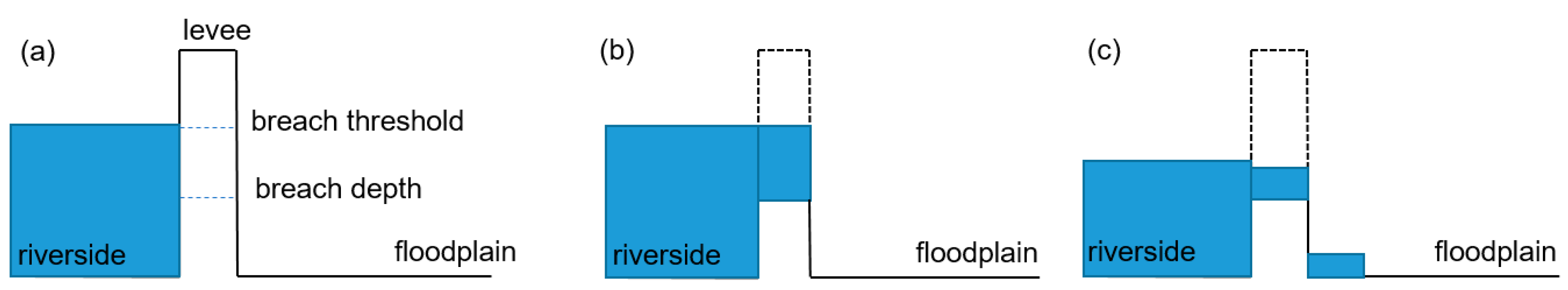
The computational sub-routine evaluates two simple breaching conditions: (i) water levels exceed threshold height and (ii) water levels stay above threshold for a defined amount of time. The procedure of breach initialization and subsequent water flow simulation is schematically shown in Figure 1.

The following parameters need to be specified for the initiation of a breach: breach location, breach threshold, duration threshold, and breach depth relative to the crest height. These parameters are further discussed in more details.

Breach location is specified by x and y coordinates of a grid cell where breach may occur. For this, the levee needs to be explicitly represented in the input DEM with the corresponding location and height. Threshold level is the water level in meters which needs to be exceeded for breach initiation. Duration threshold is the time in seconds during which the threshold water level at the levee is exceeded. Breach depth is the depth in meters in relation to the levee crest height assigned upon the breach initiation. The levee breaches instantaneously, i.e., once the breach conditions are met, the breach depth is set to the pre-defined value.

If the breach conditions are fulfilled, the levee breach at the pre-defined location is simulated in all indicated directions. The outflow discharge ($Q$) is calculated using the broad-crested weir equation:

$$Q=C\times L\times H^{1.5}$$

(1)

where, C is a weir flow coefficient, L is levee breach width (m) and H is the energy head upstream (m) [31]. In a simplified form, the water depth above weir crest upstream of the breach is considered instead of energy head ($h_u$). The numerical stability of the sub-routine is mainly controlled by the modular limit (user-defined value), which automatically switches between the free flow over a broad-crested weir Equation (1) and the drowned weir flow (Equation (2)):

$$Q=C\times L\times h_u\sqrt{\frac{h_u-h_d}{M}}$$

(2)

where $h_u$ and $h_d$ are water depths above the weir crest upstream and downstream from the breach, respectively, while M is modular limit. The value of M is selected by the user and is constant for the course of simulation. The typical range depends on the head upstream (water height relative to the bed elevation) and the final elevation of the breached embankment [32].

Weir equation (Equation (2)) is the most common approach to simulate flow through dike breaches [33]. This approach is mass conservative, but no momentum transfer from the channel into the floodplain is considered.

The minimum breach width for one grid cell is equal to the input DEM cell width. In case the specified breach width is larger than the input DEM resolution, the required amount of neighbouring cells must be specified as potential breach cells including both threshold parameter and breach depth. The equation is then solved for each cell separately.

The current configuration uses a simple set of conditions with which failure due to various breach mechanisms can be mimicked. For instance, in case of overtopping, the user can specify the breach threshold height at the levee crest. Further, the duration threshold of overtopping flow can be set. Once a failure occurs, the breach depth defined by the user is reached instantaneously. Failure due to piping/erosion (“manual” failure) can be mimicked by adjusting the breach threshold height and duration. For the reconstruction of historical events, if the time between the start of the piping process and the collapse of a levee is known, the duration threshold can be set accordingly.

We assume that the ultimate breach width has a larger impact on hazard characteristics than the width development rate, in particular for large-scale studies. This is a common assumption that has been adopted elsewhere, e.g., [25].

2.2. Synthetic Test Description

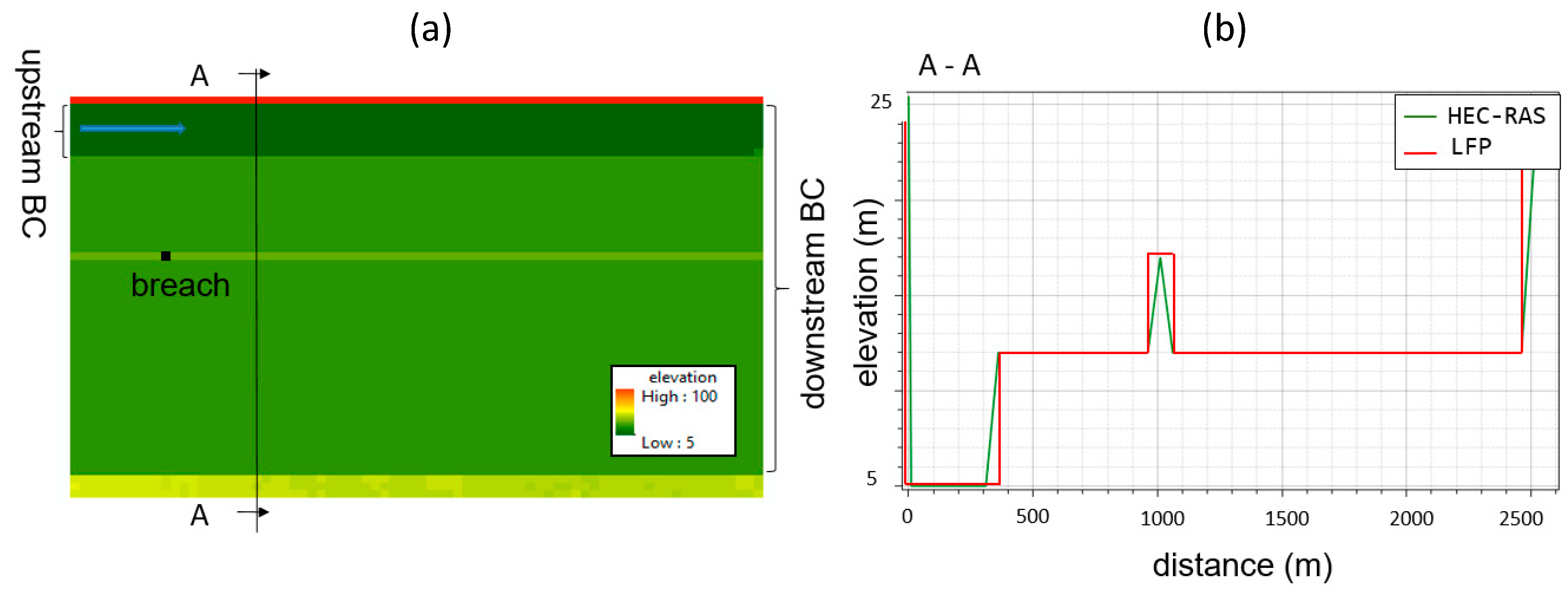
In order to evaluate the performance of the levee breaching module, we set up a series of synthetic tests. As the reference for these tests, we perform simulations with the 2D model set up using HEC-RAS (version 5.0.3, [34]). It uses either the full momentum shallow water equation or a diffusive wave approximation. For our tests we selected the first approach, as recommended in [34]. HEC-RAS has proved to be a reliable tool to simulate hydraulic processes within river channels and floodplains (water surface elevations, velocities, arrival time, etc.), including representation of various hydraulic structures (dams, levees, bridges, culverts, etc.). It allows flood parameters to be obtained with a high level of accuracy and detail [34,35]. Levee breach simulation with HEC-RAS was undertaken in numerous studies [15,28,36]. The flow through the breach is calculated using a broad-crested weir equation (same as used in the presented module) [34]. The 2D breaching link is represented as a lateral structure which connects both 2D areas, riverside and floodplain. Another relevant distinction is that HEC-RAS simulations were found up to 20 times slower than LISFLOOD-FP runs using the same resolution and domain size [35]. We specify a synthetic terrain model, inflow discharges, and downstream boundary conditions (Figure 2 and Figure 3).

Synthetic tests for HEC-RAS and LISFLOOD-FP models were built to compare the breach outflow on a simple terrain. The synthetic DEM was designed to include a river channel with an adjacent floodplain, a levee (5 m crest height) and the floodplain behind the levee (Figure 2).

While LISFLOOD-FP operates with a spatially uniform square mesh, which is at the same resolution as input raster grid, HEC-RAS internally processes terrain data into a Triangulated Irregular Network (TIN) file thus making slopes smoother. Therefore, the terrain profiles look different (Figure 2) and this may influence the flow propagation. The parameterization of the breach module is set as follows: breach threshold is set to 2 m below the levee crest height, duration threshold equals to 10 s, breach depth was set to 2 m, and the modular limit equals 0.5.

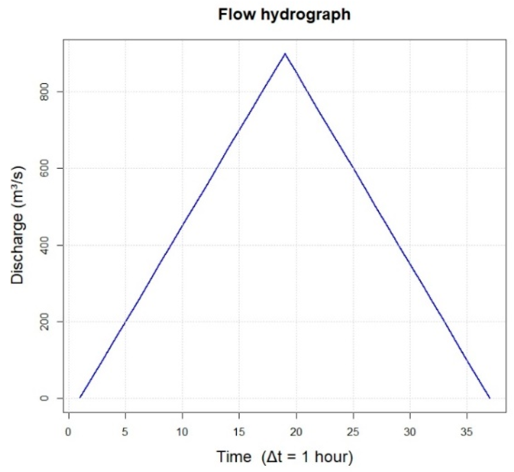
Several simulation runs using different roughness coefficients in the range 0.03–0.1 $\mathrm{s}/{\mathrm{m}}^{1/3}$, with sampling step of 0.01 $\mathrm{s}/{\mathrm{m}}^{1/3}$ were performed. The model inflow hydrograph (Figure 3) was generated in such a way that in the absence of a breach the flood waters would not overtop the levee. The simulation time was set to 35 h with 3 s time step.

We compared LISFLOOD-FP and HEC-RAS performance in terms of the breach outflow i.e., hydrograph shape and the peak flow differences. To improve model stability, the maximum Froude number was set to 1 for LISFLOOD-FP simulations, meaning the model is limited to subcritical and critical flows in this and all subsequent cases.

2.3. Secchia Inundation

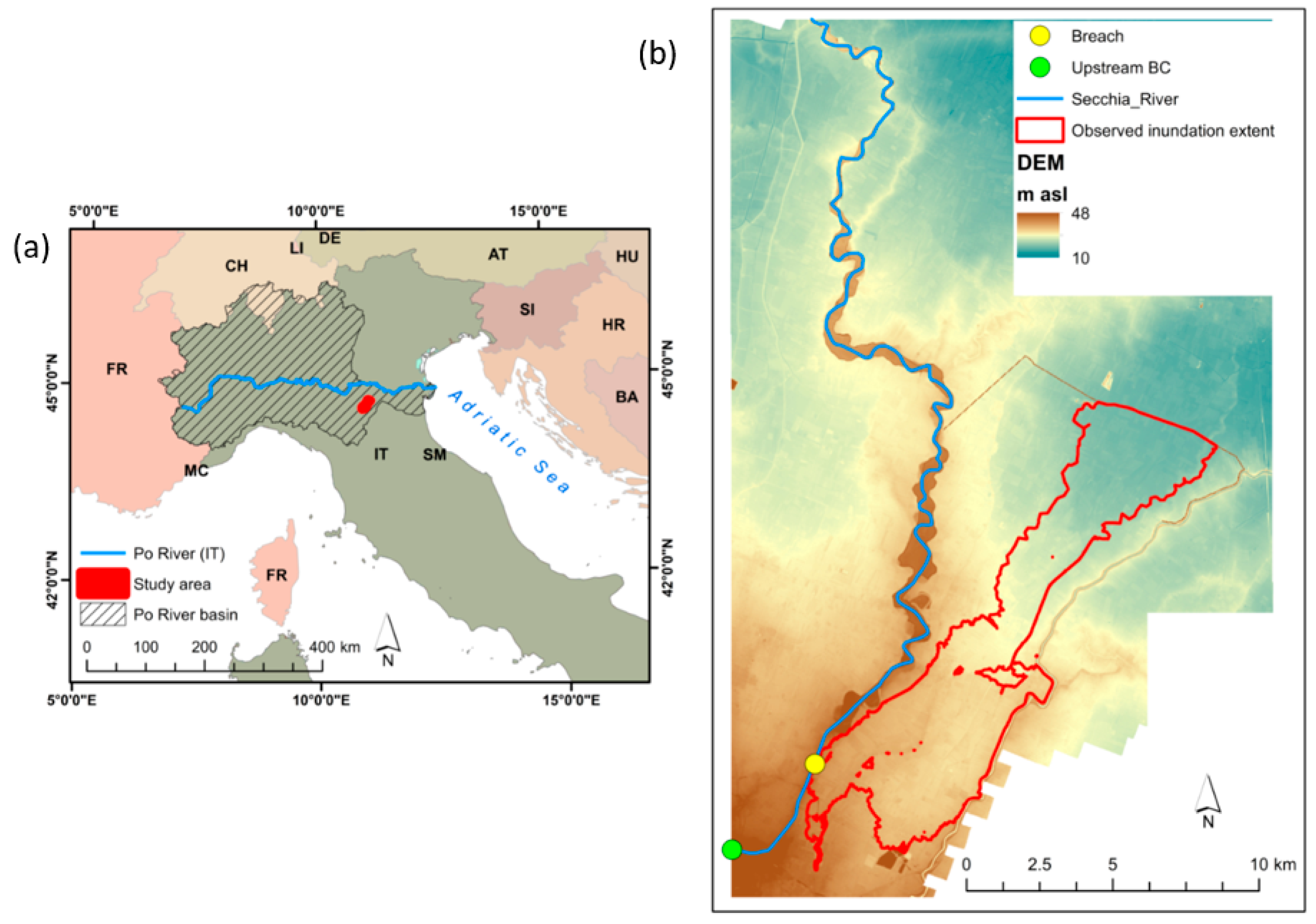
In addition to the synthetic test, we used the new LISFLOOD-FP module to simulate a historical flood event that occurred on the Secchia River (right bank tributary of the Po River) in January 2014. This case study was selected to test the sensitivity of the model parameters. During this event, approximately 50 km² of the protected floodplain was inundated as a consequence of a levee breach, causing a damage in excess of 400 million Euro and 2 fatalities. The water level at the levee did not exceed the design return period, so the levee was not overtopped. Post-event surveys concluded that the levee failed due to the lack of maintenance and burrowing animal activity, which resulted in erosive processes and followed by a lowering of the crest [37]. The final breach depth reached the ground level. The full breach evolved within 9 h and reached 80 m in width. The total outflow volume was estimated around 39 million m³ [38].

In this test we aim to reproduce the 2D flow within the Secchia River channel, breach and consequent inundation of the initially dry floodplain (Figure 4). We use a LiDAR DEM of 1 m resolution which represents the bare earth terrain with buildings and vegetation removed. It includes the bathymetry of the riverbed and levees with a vertical accuracy of ±0.15 m. We aggregate the DEM to 25 m horizontal resolution, using the mean value of the 1 m pixels. The levee is represented by ‘burning’ it into the 25 m DEM, i.e., the actual levee crest elevation is assigned from the 1 m LiDAR data to respective cells of the aggregated DEM. The resulting number of raster cells in the model domain was about 888,000. Additionally, we burnt in an embankment downstream from the breach (northern part of the domain) into the DEM, where the flood accumulated due to the elevated ground, as was reported by the post-event survey [39]. The relief of the study area is characterised by highly heterogeneous terrain with a complex network of irrigation canals and embankments.

The upstream boundary condition for the Secchia river is assigned ca. 5.5 km upstream from the breach, where a gauging station is located (Figure 4). The input hydrograph at this location was obtained from [38]. The event simulation time was 100 h with a maximum time step of 5 s. Downstream boundary condition was set where the Secchia River confluences with the Po River and set as a free boundary.

We identified the breach location from the post-event surveys and assigned corresponding three cells in the LISFLOOD-FP meaning the breadth equalled to 75 m (observed width was 80 m). The breach depth was assigned to reach the ground level. Because the breach was caused by an erosive process, not overtopping, we adjusted the flood breach time manually according to historical observations. The levee failure extension was settled in order to reproduce the failure when the hydraulic condition (i.e., water level) within the river was equal to observations.

We investigated the sensitivity of the LISFLOOD-FP model to different modular limits. Additionally, we looked into the interaction between different values of the modular limit and the floodplain roughness coefficient in the area immediately behind the breach. Altogether, we ran 135 simulations of all possible configurations of modular limit (0.1, 0.2… 0.9 $\mathrm{s}/{\mathrm{m}}^{1/3}$) and floodplain roughness coefficients (0.03, 0.035, 0.4 … 0.1 $\mathrm{s}/{\mathrm{m}}^{1/3}$).

The performance of the model simulation was assessed by comparing the simulated and previously estimated outflow discharge [38] using the Nash–Sutcliffe model efficiency coefficient (NSE):

$$NSE=1-\frac{{{\displaystyle \sum }}_{t=1}^T{\left(Q_m^t-Q_O^t\right)}^2}{{{\displaystyle \sum }}_{t=1}^T{\left(Q_O^t-{\overline{Q}}_O\right)}^2}$$

(3)

where $Q_m^t$ is simulated outflow, $Q_O^t$ estimated outflow, and ${\overline{Q}}_O$ is the sample mean of estimated outflow at each time step. The riverbed was assigned a calibrated Manning’s n value of 0.015 $\mathrm{s}/{\mathrm{m}}^{1/3}$.

Another aspect of model performance that we tested once the model was calibrated was the ability to reproduce the inundation boundary and water depth in the floodplain behind the breached levee. For this purpose, we looked into previous research and post-event surveys done to describe and analyse this event. In particular, we referred to the flood extent estimated in a previous study [11]. Carisi et al. [11] reconstructed the event reaching 90% Critical Success Index (CSI, see Equation (4)). These data were used as a benchmark to evaluate the simulated inundation extent. We selected the CSI to assess the match of the simulated and observed inundation extent.

$$F=\frac{A}{A+B+C}\times 100$$

(4)

where A represents the area being flooded according to both the model and observations (true positive), B is the overestimated area by the model (false positive) and C is the underestimated area by the model (false negative). CSI of 0 indicates no overlap between the model and observations and CSI of 100% corresponds to a perfect fit between modelled and observed inundation extent.

Additionally, we looked into the spatial distribution of water depth at available control points, which were obtained from the field surveys done by the local municipalities and publicly available photographs of the water and wreck marks. Such measurements are known to be prone to errors, which could reach up to 0.5 m [40]. Altogether, there were 46 such control points, which are mostly located within the towns of Bastiglia and Bomporto. We analysed the ability of the models to predict these water elevations using root mean square error (RMSE). These and all consequent simulations were performed on a server with 2 CPUs having 20 real cores and hyperthreading 40 cores.

2.4. November 1951 Polesine Catastrophic Flood of the Po River

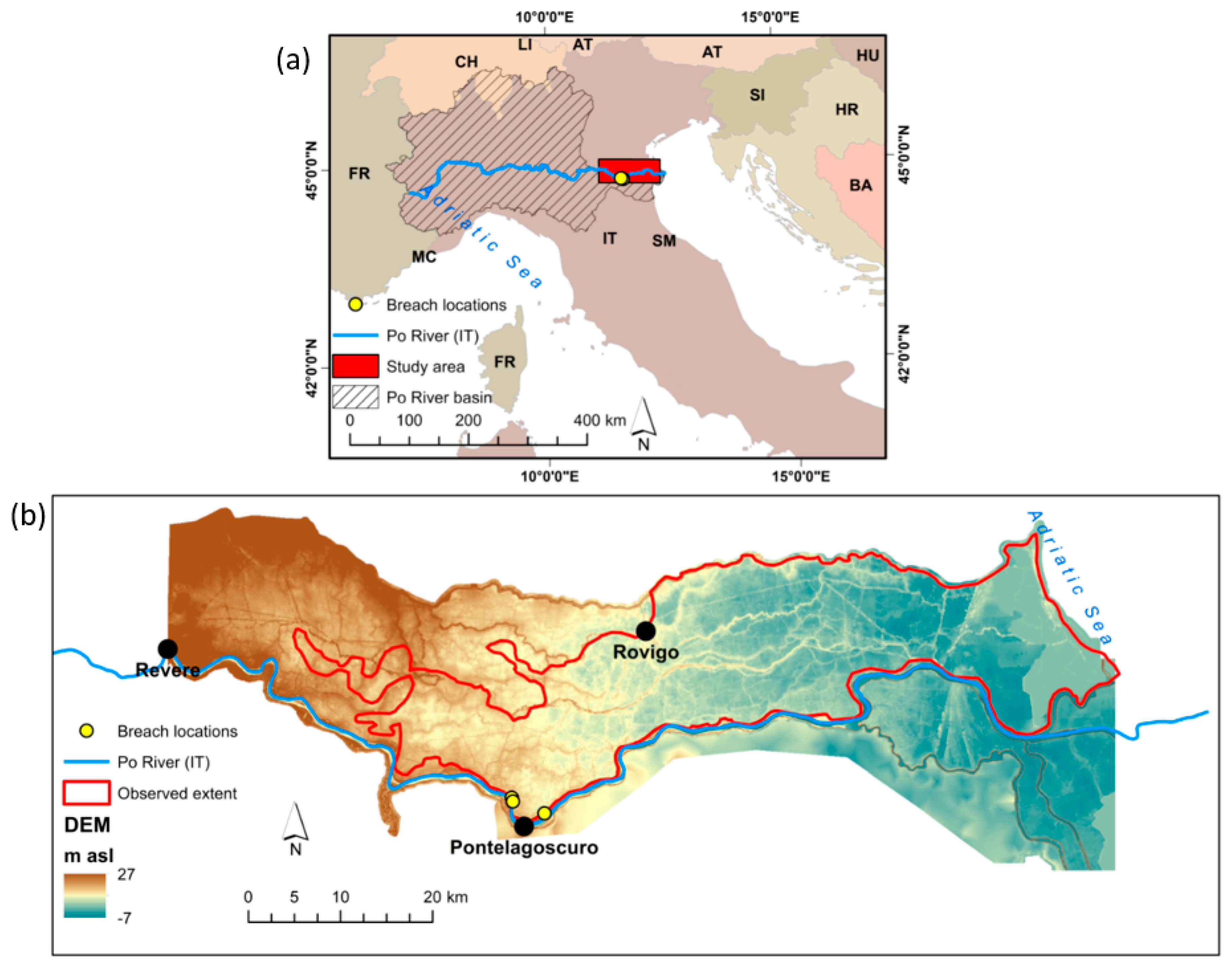
In order to test the LISFLOOD-FP model on more extreme events for geographically larger areas and evaluate its computational efficiency and accuracy, we simulated the catastrophic Polesine riverine flood, which occurred in November 1951 on the Po River (Northern Italy). During this event, an unusually massive rainfall generated extreme discharges on the Po river reaches [41]. About 50 km upstream from the river mouth (at the Pontelagoscuro gauging station, Figure 5), the left levee of the main channel was overtopped, and then eventually breached at 3 different locations. The ultimate breach width reached the width between 200 and 300 m.

The flood waters inundated over 1000 km² of protected floodplain, eventually reaching the shore of the Adriatic Sea. The event caused 114 deaths, long lasting population displacement, about $7.8 billion monetary losses (in 2018 dollar values) and catastrophic impact on local ecosystems [41]. Recent studies by [41,42] together with historical reports provide an overview of the event.

For the LISFLOOD-FP model setup, the upstream boundary condition was generated based on the report by [43], while some of the breaching parameters were retrieved from [42], who specified the location of the three breaches and their final width. The latter values were 220, 204 and 312 m, which in our set up were represented as breaches of 250, 200 and 300 m wide respectively. The reconstruction of the terrain data corresponding to the state of 1951 is challenging given that anthropogenic changes have triggered land subsidence of up to 3 m in the coastal part of the model domain [41]. However, the study of [11] pointed out that manmade alterations that mostly influence flood hazard over large floodplains are generally linear infrastructures. Viero et al. [41] reports that some of the embankments were raised and new embankments were constructed in the aftermath of the event. We use terrain data from 2004 (river channel bathymetry) and 2011 (floodplain) survey (both datasets are provided by the Po River Basin Authority, www.adbpo.it). We resampled 2 m resolution LiDAR data to 50 m resolution DEM and imposed the actual height of the embankments taken from LiDAR survey onto the resampled DEM. In this approach, the effect of the linear structures (embankments) on the flow propagation within the main channel is explicitly considered. Since we use the terrain data including levee locations which do not exactly correspond to the state of 1951, we expect certain dissimilarities, especially in the areas around newly built embankments. Because the exact levee geometry could not be reproduced due to differences in terrain between the event occurrence (1951) and data acquisition (2011), we set up the model according to the current elevations (2011). This means that the crest height, the breach depth relative to crest height and adjacent bathymetry were as of 2004/2011. We simulate the Polesine flood event in the fully 2D mode. As for the Secchia event study, we model the whole chain of the event including the 2D river flow, levee breaching and weir overflow and subsequent floodplain inundation. The upstream boundary condition is set up at the Revere gauging station (Figure 5), while downstream was at the Adriatic Sea. First, we calibrated the model against the reported discharge values at the Pontelagoscuro gauging station [43] using a spatially uniform channel roughness coefficient where the breaches are not considered in the simulation. Afterwards, we set up the breaching locations and widths as reported in [42]. The threshold height is set to the levee crest height and the failure occurs instantaneously. The breach time was adjusted to allow simultaneous breach at all 3 locations. The simulation duration was set to 348 h, of which first 61 h were a warm-up with a maximum time step of 5 s. The breaching depth was set to 7 m at all locations and the modular limit of 0.5 was selected by trial and error method in order to let the simultaneous breach at all indicated locations. The approximate extent of the flood is known from the previous studies of [41], which is reported to have 88% accuracy (CSI). These data are used here to evaluate the model performance using CSI (4).

3. Results

3.1. Synthetic Tests

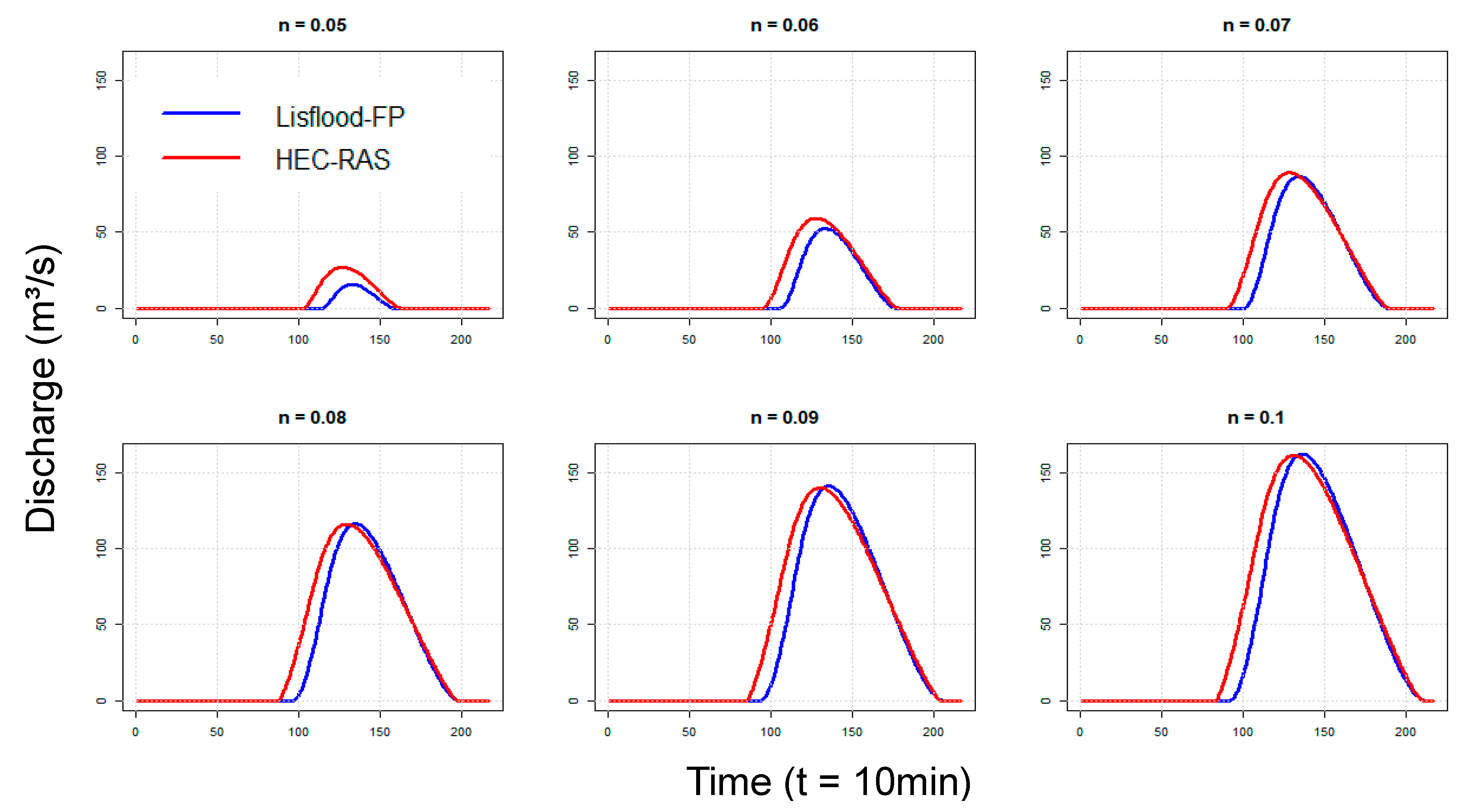
In the synthetic tests, the breach occurred for simulations where the roughness coefficient of the floodplain was more than 0.05 $\mathrm{s}/{\mathrm{m}}^{1/3}$. For lower roughness coefficients the breach was not activated because the triggering hydraulic conditions were not met. The shape of the outflow hydrographs is similar for both models for all roughness coefficients (Figure 6). In LISFLOOD-FP simulations, the breach occurs about 1 h later than in HEC-RAS. The absolute difference in the discharge peaks is rather insignificant, considering the inflow discharge. For n = 0.05 and 0.06 the LISFLOOD-FP peak is 7% lower than HEC-RAS, whereas for 0.07, 0.08, 0.09, and 0.1, both models perform identically for this parameter (difference is less than 1%). The computation time for LISFLOOD-FP simulations was nine times faster than for identical set-up of HEC-RAS.

3.2. Secchia Inundation

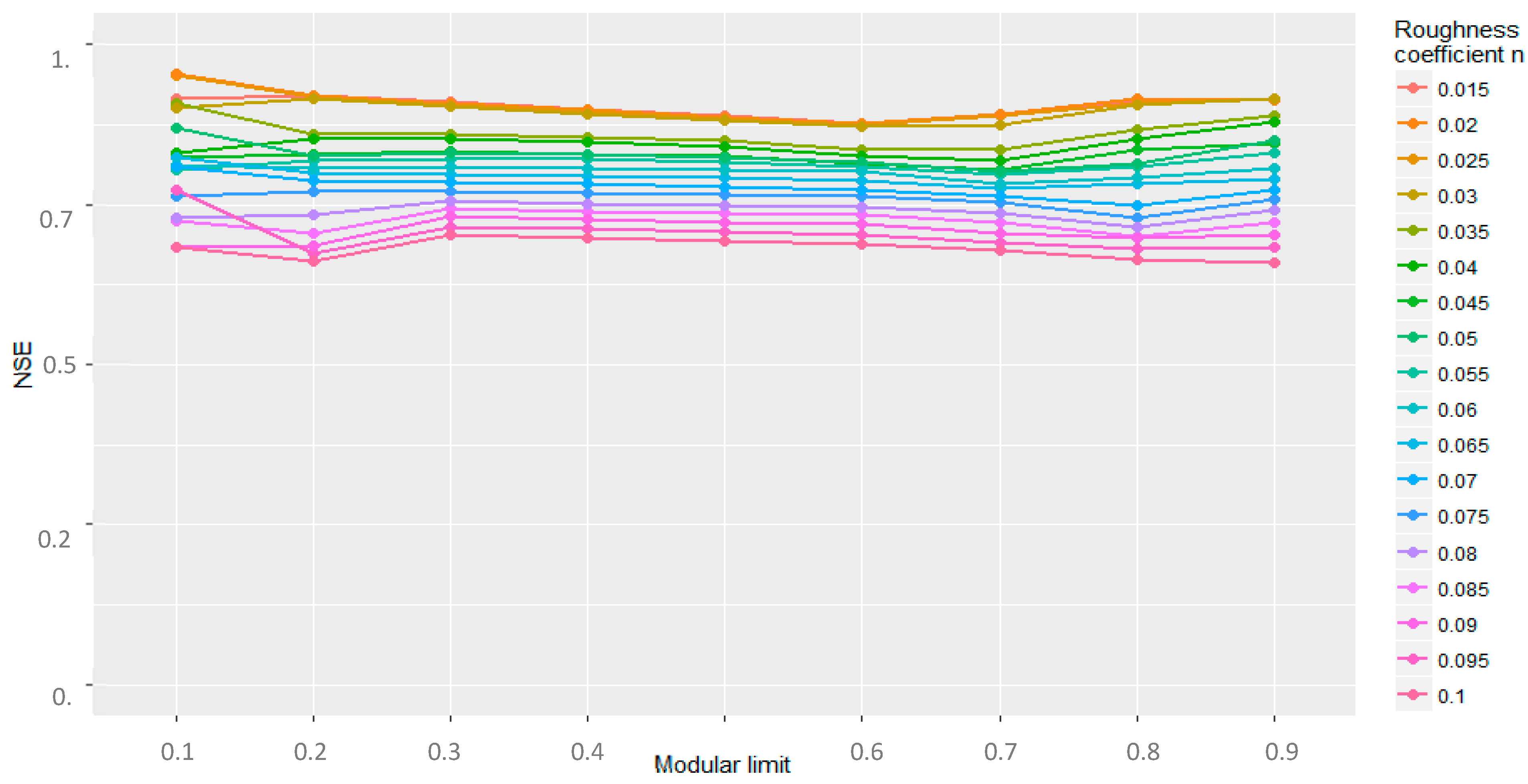
As outlined in the Methods section, the aim of this case study was to analyse the performance of the breach module on a complex terrain for a historic event and explore the sensitivity to various model parameters. In Figure 7, the performance with regards to the simulated outflow is evaluated depending on the roughness coefficient and modular limit. The outflow discharge is more sensitive to variations in the roughness parameters compared to variations in the modular limit. The difference between NSE values obtained for the set of modular limits within each roughness coefficient (i.e., modular limits 0.1–0.9 run with 0.03 $\mathrm{s}/{\mathrm{m}}^{1/3}$) are in the range of 0.05–0.07. In contrast, the variation of NSE for different roughness coefficients and the same modular limit is in the range of 0.32 (as a maximum value). The NSE slightly increases for lower Manning values, becoming nearly stable at <0.025 $\mathrm{s}/{\mathrm{m}}^{1/3}$. For lower roughness values (<0.015 $\mathrm{s}/{\mathrm{m}}^{1/3}$) LISFLOOD-FP becomes numerically unstable in calculating the flow leaving. As can be seen from Figure 7, there is a pattern change when the modular limit is 0.1 for most of the roughness coefficients.

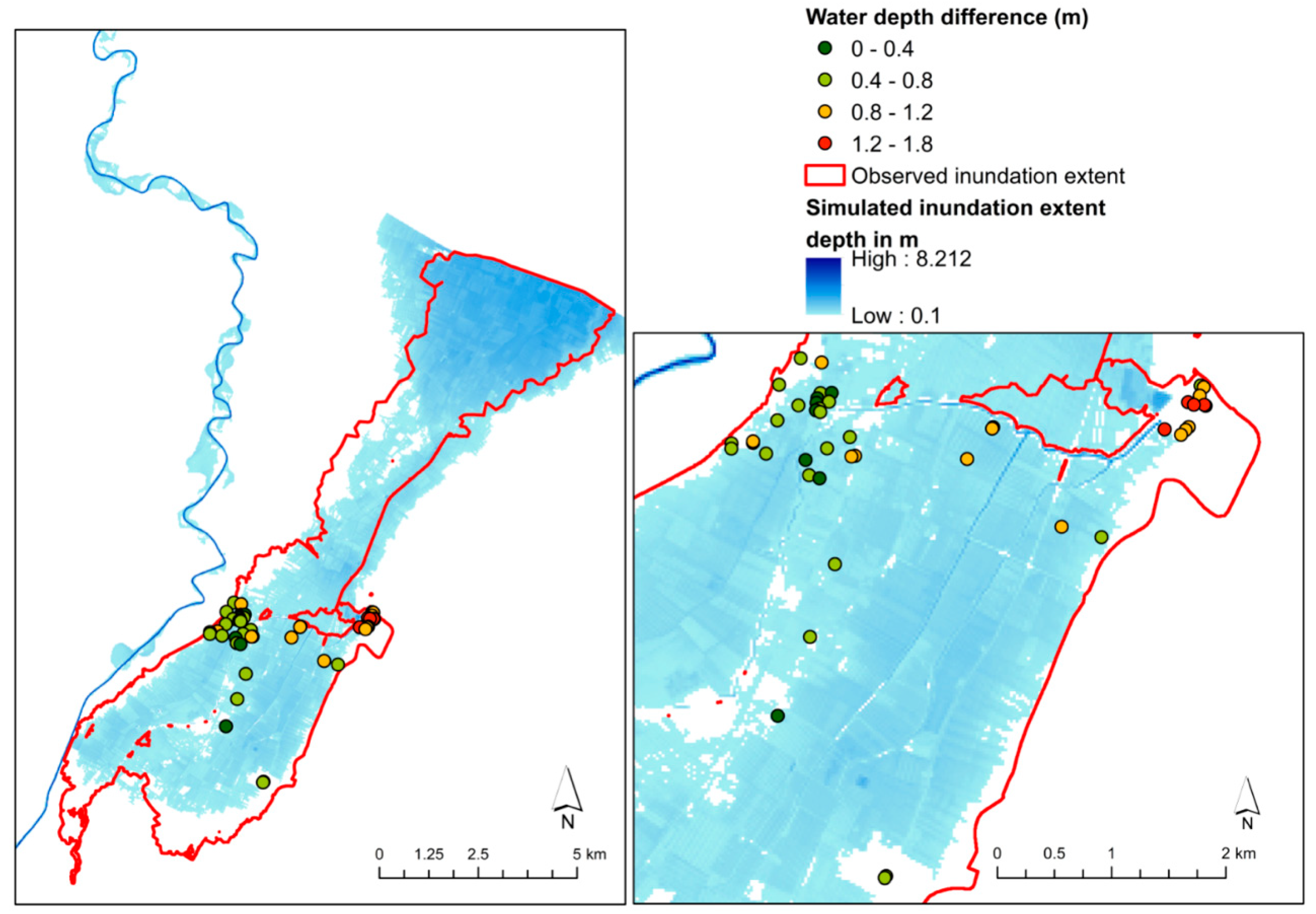
Among all simulations the best NSE value was obtained from the configuration where the modular limit was set to 0.1 and floodplain Manning value n = 0.025 $\mathrm{s}/{\mathrm{m}}^{1/3}$ (Figure 7). For this combination, the NSE coefficient reaches 0.96. Because the modular limit value is constant in each simulation, this seemingly low value (0.1) compensates for effect of changes in the upstream head over the event. Therefore, we select this configuration for further analysis. The overall volume of water leaving the breach in the selected simulation run was about 7% higher than estimated (which is 42 and 39 m³/s correspondingly). The CSI value for the best calibrated run was 64%, which shows the ability to reproduce the inundation extent (Figure 8).

The RMSE values of observed and simulated water depths at 46 points is 0.84 m (Figure 8). Horritt et al. [40] report that post-event surveys of flood water marks might have up to 0.5 m vertical error. The resulting RMSE is close to the observational error. Concerning the computation time, it took a little over three minutes to run one simulation (on a server with 2 CPUs having 20 real cores and hyperthreading 40 cores).

3.3. November 1951 Polesine Catastrophic Flood, Po River

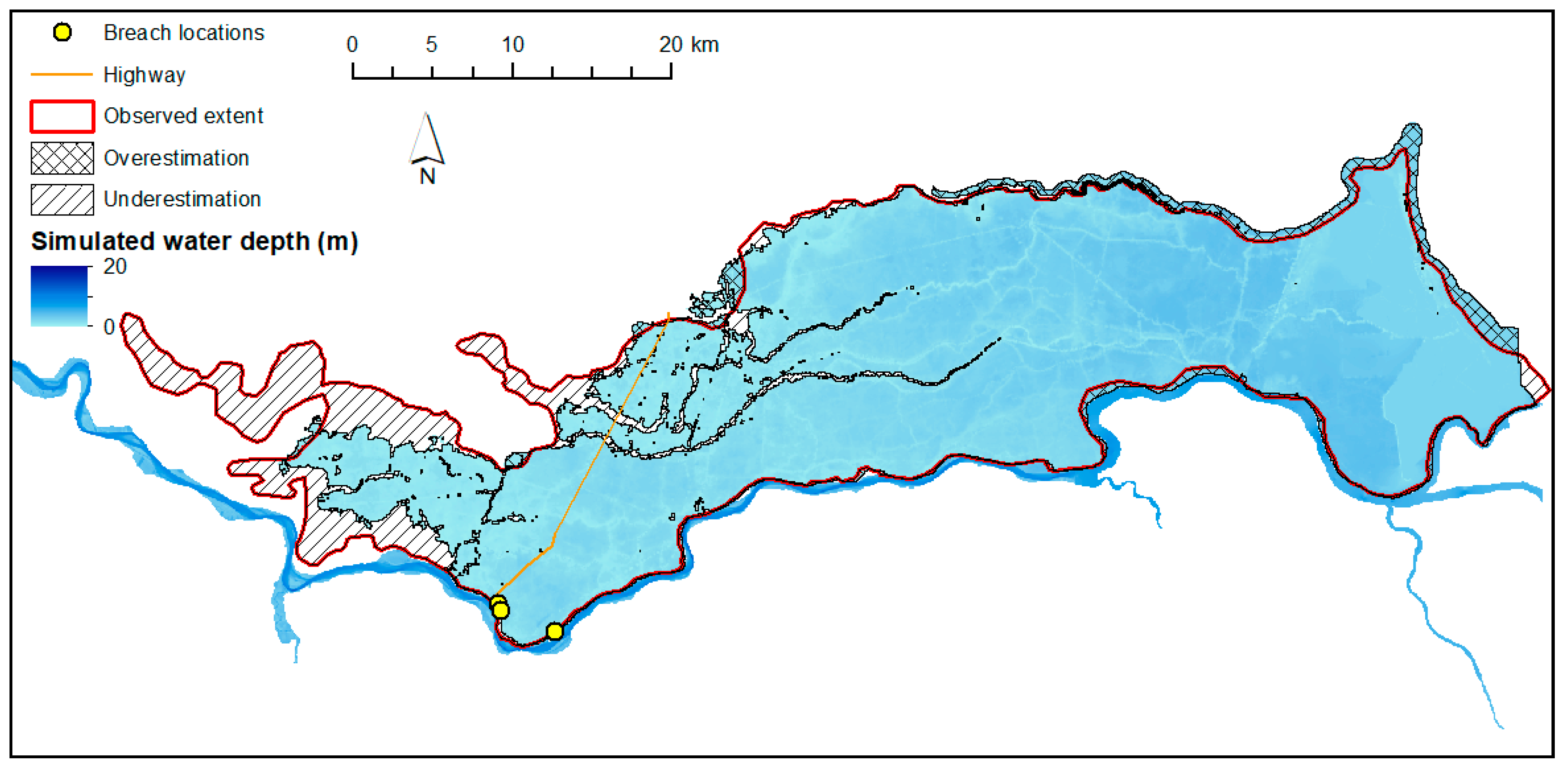
The simulations of the Polesine flood on the Po river showed that the model is able to correctly simulate the simultaneous breach of all three locations at the time reported by [41]. Due to the lack of the data on the flow leaving through the breach into the floodplain and the shape of the outflow hydrograph, we evaluated the model performance based on the inundation extent, for which more studies (i.e., [41,42]) are available. As can be seen from Figure 9, the propagation of the flood water eastwards is correctly captured by the model, which resulted in 83% accuracy in terms of the CSI for the overall flood extent compared to the surveys.

The computational time of one simulation of 348 h and over 1,620,000 cells of the input domain with a maximum time step of 5 s was about 50 min.

4. Discussion

The new levee breaching sub-routine of LISFLOOD-FP was tested on a number of synthetic and real case scenarios.

4.1. Synthetic Cases

First, we identified that the new extension behaves similarly to the breach module of the HEC-RAS 5.0.3 model under synthetic conditions. Outflow hydrographs using various roughness values had similar patterns in the two models. The peak flow differences were less than 1% for most of simulations. Largely because the same equation is used to calculate the flow leaving through the breach (see Methods section). The slight differences between the two models might be explained by their rather different formulations used to calculate floodplain flow (inertial formulation of the shallow-water equation in LISFLOOD-FP and full momentum equation in HEC-RAS) and correspondingly different peak flow in the hydrograph in main channel.

For unsteady flow simulations (triangular hydrograph, Figure 3), we obtained a definite pattern, where under identical set ups and breaching conditions, the levee fails about an hour later for all simulations in LISFLOOD-FP compared to HEC-RAS. This is due to the differences in channel and floodplain flow to the breach location, which, as mentioned above, is computed using different terms. For lower roughness coefficients (<0.6 $\mathrm{s}/{\mathrm{m}}^{1/3}$) the difference in the peak flow is the largest, while for the higher ones the peak flow is virtually identical. Also, the roughness coefficient controls the water level in the river channel and the adjacent floodplain and thus the water height above the levee toe. Higher water levels at higher roughness conditions lead to a stronger breach outflow discharge.

The tests demonstrated the reliability of the new breach module in LISFLOOD-FP under different conditions on simplified terrain and also shows the potential to calibrate the models to obtain identical results. Moreover, the computation time difference showed an obvious advantage of LISFLOOD-FP over HEC-RAS. Computation time plays a crucial role in large-scale flood modelling and is a rather particularly remarkable burden in 2D large-scale simulations.

4.2. Historic Events Simulations

Concerning more complex configurations, we looked at the embankment failure that occurred on the Secchia River. There, we aimed at simulating the whole chain of the flood event starting from the flow ca. 5.5 km upstream of the breach, the failure and the floodplain inundation using the new module of LISFLOOD-FP. Notwithstanding the heterogeneity of the terrain in the area, which potentially might have become a source of inaccuracies, LISFLOOD-FP produced credible outcomes. The overall volume through the breach was overestimated by 7%. The flood extent in the protected floodplain was predicted with 64% accuracy (using a critical success index metric) and the water elevation at a set of control points was predicted with RMSE = 0.84 m. A high complexity of floodplain terrain would require much more deliberate calibration using spatially variable roughness coefficients. Moreover, a raster-based model with 25 m resolution would not be able to include fine linear features of the terrain such as embankments and canals, which are in some cases not more than 5 m wide. We suggest that in order to address these points, additional calibration of the floodplain roughness coefficients should substantially improve the flood extent fit, however this was not the goal of the sensitivity analysis. Moreover, the current study was not deliberately assessing the uncertainties related to the input data, nevertheless, it is worth mentioning that there are possible ambiguities related to the DEM vertical accuracy and likely errors in the water evaluation control points.

In some simulations, low modular limits of 0.1 provided numerically unstable calculations of the flow leaving the breach with the large portion of backwater effect at the time point when it is not supposed to occur. The tests have shown that such instabilities can be solved by the change of modular limit. Based on sensitivity analysis and synthetic tests, we found that modular limit values between 0.2 and 0.8 produce numerically stable simulations. Moreover, very low Manning roughness coefficients (<0.015) used in the area adjacent to the breach should be avoided due to instability issues.

Due to the lack of detailed bathymetry and terrain data from 1951, the model was set up according to modern geometries (breach depth and width). LISFLOOD-FP reached sufficient accuracy in simulating the whole chain of the event: extreme water levels within the channel, simultaneous breach at multiple pre-defined locations and consequent inundation of the floodplain. Investigating the floodplain flow propagation, we gained substantial accuracy of 83%. Viero et al. [41] in their study attained 86%–88% accuracy by using a DEM which does not contain anthropogenic changes imposed since 1951. However, the model was not able to simulate inundation in the western part of the domain. This was expected due to the terrain topography which lowers to the east, closer to the vicinity of the coast. The changes in terrain elevation between 1951 and 2004/2011 are rather prominent in the western part of the model domain [41]. As mentioned above, some of the embankments were built after 1951; one of them crossing from north to south and acted in our simulation as a flood boundary (See brown line in Figure 9).

We suspect that this could explain the underprediction of inundation in the western part of the domain.

It is, however, important to specify that the reference inundation extent used to compute CSI is likely subject to biases, as it was reconstructed based on historical data and post-event field surveys [41]. From this test we could see that the sub-routine is numerically stable for a geographically large simulation with multiple breaches and was able to produce reasonable outcomes.

4.3. Assumption and Limitation of the Levee Failure Extension

Alongside the module flexibility and rather simple set-up, there are certain aspects of the newly developed module that are worth highlighting. First and foremost, the input DEM has to include important elements, such as the levee location and crest height. In many instances the levee height and location data can be unavailable. However there are options being developed to extract levee locations and height from the remotely sensed images, available geodata (OpenStreetMap [44]) cadastral data. Some methods would include DEM-based algorithms [45,46,47]. The increasing availability of LiDAR surveys should make levee extraction more feasible for flood modellers in the future.

Another important aspect is that the assumed breach shape is rectangular and expressed as a multiple of the raster resolution. For large scale modelling, which is sometimes run at the 100 m resolution and coarser, the minimum breach width might be an overestimation. Numerous studies on the breach modelling have shown the importance of a detailed description of the geometry of the breach, which in most cases is either rectangular or trapezoidal [16,33]. In our study, we assume that for large scale studies, where the breach width would range from 25 m up to hundreds of meters, such complication for the model is negligible. The levee thickness is defined by the terrain resolution, meaning, if the input DEM resolution is 50 m, the levee is 50 m wide.

Another point to consider is that breach occurs instantaneously, meaning, the breach width starts developing as soon as the breaching conditions are met. For long-term simulations at large scale, we might neglect the breach evolution over time [48].

Moreover, the model does not account for sediment transport and rapid changes in the riverbed due to morphodynamic processes. Therefore, in cases where the flow is expected to be largely impacted by the above-mentioned factors, the breaching module of LISFLOOD-FP should be replaced by a morphodynamic model. The tool is not meant for detailed engineering studies of the breaching phenomenon and should be used for regional and large-scale hazard and risk assessments. However, in case there is supercritical flow expected, full-momentum models should be applied.

5. Conclusions

This paper presents a new levee-breaching extension within the widely used model LISFLOOD-FP for simulating flood breaching scenarios over geographically small and large areas, which extends the array of possible applications of the LISFLOOD-FP model. Levee breaching is a useful component for hydrodynamic models to replicate the complex interaction between the river channel and floodplains in 2D mode. The tests shown in this paper prove that the extension is capable to reasonably simulate historical flooding events. The tests on various domain sizes and different magnitudes of hydrological forcing proved that the module is able to capture the flow leaving the breach and reproduce the interactions between the river channel and protected floodplains. Given the computation time of the Secchia river flood simulations (about three minutes) and the rather large number of computational cells (880,000), we suggest that levee breaching in fully 2D mode with LISFLOOD-FP can be performed in Monte Carlo simulations for the probabilistic flood mapping. The same conclusion also applies for larger study areas as demonstrated by the Polesine flood simulations. Compared to the already existing tool (i.e., HEC-RAS), which allows levee-breaching in fully 2D mode, LISFLOOD-FP is much more computationally faster. The ability to quickly yet efficiently simulate levee failure and consequent inundation of the protected floodplain in 2D mode may be of great use for flood risk modellers and decision-makers, as the calculation of the residual risks is a crucial component for flood management. Such efficiency can benefit near-real time simulations and support flood management solutions in emergency cases.

Further studies should be aimed at more tests of the tool in more diverse conditions, set ups and scales, in detail investigate backwater effects. By accepting certain assumptions and performing numerous tests, we suggest that the LISFLOOD-FP breaching extension is an effective tool which will allow for levee breaching simulations on the local, regional, and large scales with the minimum set-up and computation effort.

References

- Centre for Research on the Epidemiology of Disasters. 2018 Review of Disaster Events 2019. Available online: http://www.cred.be/publications (accessed on 22 January 2020).
- Alfieri, L.; Bisselink, B.; Dottori, F.; Naumann, G.; de Roo, A.; Salamon, P.; Wyser, K.; Feyen, L. Global projections of river flood risk in a warmer world. Earth’s Future 2017, 5, 171–182. [Google Scholar] [CrossRef]
- Vorogushyn, S.; Merz, B.; Apel, H. Development of dike fragility curves for piping and micro-instability breach mechanisms. Nat. Hazards Earth Syst. Sci. 2009, 9, 1383–1401. [Google Scholar] [CrossRef]
- Marijnissen, R.; Kok, M.; Kroeze, C.; van Loon-Steensma, J. Re-evaluating safety risks of multifunctional dikes with a probabilistic risk framework. Nat. Hazards Earth Syst. Sci. 2019, 19, 737–756. [Google Scholar] [CrossRef] [Green Version]
- van Mierlo, M.; Vrouwenvelder, A.; Calle, E.; Vrijling, J.; Jonkman, S.N.; de Bruijn, K.; Weerts, A.H. Assessment of flood risk accounting for river system behaviour. International. Int. J. River Basin Manag. 2007, 5, 93–104. [Google Scholar] [CrossRef]
- De Bruijn, K.M.; Diermanse, F.L.; Van Der Doef, M.; Klijn, F. Hydrodynamic System Behaviour: Its Analysis and Implications for Flood Risk Management; EDP Sciences: Les Ulis, France, 2016. [Google Scholar]
- Ludy, J.; Kondolf, G.M. Flood risk perception in lands “protected” by 100-year levees. Nat. Hazards 2012, 61, 829–842. [Google Scholar] [CrossRef]
- Domeneghetti, A.; Carisi, F.; Castellarin, A.; Brath, A. Evolution of flood risk over large areas: Quantitative assessment for the Po river. J. Hydrol. 2015, 527, 809–823. [Google Scholar] [CrossRef]
- Andersen, C.F. The New Orleans Hurricane Protection System: What Went Wrong and Why; A report; ASCE: Reston, VA, USA, 2007. [Google Scholar]
- Larson, L.W. The Great USA Flood of 1993. 1996. Available online: https://www.nwrfc.noaa.gov/floods/papers/oh_2/great.htm (accessed on 17 February 2020).
- Carisi, F.; Schröter, K.; Domeneghetti, A.; Kreibich, H.; Castellarin, A. Development and assessment of uni- and multivariable flood loss models for Emilia-Romagna (Italy). Nat. Hazards Earth Syst. Sci. 2018, 18, 2057–2079. [Google Scholar] [CrossRef] [Green Version]
- Vorogushyn, S.; Bates, P.D.; de Bruijn, K.; Castellarin, A.; Kreibich, H.; Priest, S.; Schröter, K.; Bagli, S.; Blöschl, G.; Domeneghetti, A. Evolutionary leap in large-scale flood risk assessment needed. Wiley Interdiscip. Rev. Water 2018, 5, e1266. [Google Scholar] [CrossRef] [Green Version]
- Sanders, B.F.; Pau, J.C.; Jaffe, D.A. Passive and active control of diversions to an off-line reservoir for flood stage reduction. Adv. Water Resour. 2006, 29, 861–871. [Google Scholar] [CrossRef]
- Vorogushyn, S.; Lindenschmidt, K.-E.; Kreibich, H.; Apel, H.; Merz, B. Analysis of a detention basin impact on dike failure probabilities and flood risk for a channel-dike-floodplain system along the river Elbe, Germany. J. Hydrol. 2012, 436, 120–131. [Google Scholar] [CrossRef] [Green Version]
- Castellarin, A.; Domeneghetti, A.; Brath, A. Identifying robust large-scale flood risk mitigation strategies: A quasi-2D hydraulic model as a tool for the Po river. Phys. Chem. Earth Parts A/B/C 2011, 36, 299–308. [Google Scholar] [CrossRef]
- Viero, D.P.; D’Alpaos, A.; Carniello, L.; Defina, A. Mathematical modeling of flooding due to river bank failure. Adv. Water Resour. 2013, 59, 82–94. [Google Scholar] [CrossRef]
- Wu, W. Earthen Embankment Breaching. J. Hydraul. Eng. 2011, 137, 1549–1564. [Google Scholar] [CrossRef]
- Dazzi, S.; Vacondio, R.; Mignosa, P. Integration of a Levee Breach Erosion Model in a GPU-Accelerated 2D Shallow Water Equations Code. Water Resour. Res. 2019, 137, 1549. [Google Scholar] [CrossRef]
- Morris, M.W.; Kortenhaus, A.; Visser, P.J.; Hassan, M. Breaching Processes. 2009. Available online: http://www.floodsite.net/html/publications2.asp?by=documentDeliverables&byway=desc&documentType=1 (accessed on 19 March 2020).
- Zhong, Q.; Wu, W.; Chen, S.; Wang, M. Comparison of simplified physically based dam breach models. Nat. Hazards 2016, 84, 1385–1418. [Google Scholar] [CrossRef]
- Teng, J.; Jakeman, A.J.; Vaze, J.; Croke, B.; Dutta, D.; Kim, S. Flood inundation modelling: A review of methods, recent advances and uncertainty analysis. Environ. Model. Softw. 2017, 90, 201–216. [Google Scholar] [CrossRef]
- Hunter, N.M.; Bates, P.D.; Horritt, M.S.; Wilson, M.D. Simple spatially-distributed models for predicting flood inundation: A review. Geomorphology 2007, 90, 208–225. [Google Scholar] [CrossRef]
- Chatterjee, C.; Förster, S.; Bronstert, A. Comparison of hydrodynamic models of different complexities to model floods with emergency storage areas. Hydrol. Process. 2008, 22, 4695–4709. [Google Scholar] [CrossRef]
- Kamrath, P.; Disse, M.; Hammer, M.; Köngeter, J. Assessment of Discharge through a Dike Breach and Simulation of Flood Wave Propagation. Nat. Hazards 2006, 38, 63–78. [Google Scholar] [CrossRef]
- Vorogushyn, S.; Merz, B.; Lindenschmidt, K.-E.; Apel, H. A new methodology for flood hazard assessment considering dike breaches. Water Resour. Res. 2010, 46, 125. [Google Scholar] [CrossRef] [Green Version]
- Rodríguez-Blanco, M.L.; Taboada-Castro, M.M.; Taboada-Castro, M.T. Factors controlling hydro-sedimentary response during runoff events in a rural catchment in the humid Spanish zone. Catena 2010, 82, 206–217. [Google Scholar] [CrossRef]
- Luke, A.; Kaplan, B.; Neal, J.; Lant, J.; Sanders, B.; Bates, P.; Alsdorf, D. Hydraulic modeling of the 2011 New Madrid Floodway activation: A case study on floodway activation controls. Nat. Hazards 2015, 77, 1863–1887. [Google Scholar] [CrossRef]
- Mazzoleni, M.; Bacchi, B.; Barontini, S.; Di Baldassarre, G.; Pilotti, M.; Ranzi, R. Flooding Hazard Mapping in Floodplain Areas Affected by Piping Breaches in the Po River, Italy. J. Hydrol. Eng. 2014, 19, 717–731. [Google Scholar] [CrossRef]
- Bates, P.; Horritt, M.S.; Fewtrell, T.J. A simple inertial formulation of the shallow water equations for efficient two-dimensional flood inundation modelling. J. Hydrol. 2010, 387, 33–45. [Google Scholar] [CrossRef]
- Neal, J.; Villanueva, I.; Wright, N.; Willis, T.; Fewtrell, T.; Bates, P. How much physical complexity is needed to model flood inundation? Hydrol. Process. 2012, 26, 2264–2282. [Google Scholar] [CrossRef] [Green Version]
- Chow, V.T. Open-Channel Hydraulics; McGraw-Hill: New York, NY, USA, 1959. [Google Scholar]
- White, W.R.; Whitehead, E.; Forty, E.J. Extending the Scope of Standard Specifications for Open Channel Flow Gauging Structures. 2000. Available online: http://eprints.hrwallingford.co.uk/891/ (accessed on 13 December 2019).
- Wu, W.; Li, H. A simplified physically-based model for coastal dike and barrier breaching by overtopping flow and waves. Coast. Eng. 2017, 130, 1–13. [Google Scholar] [CrossRef]
- Brunner, G.W. HEC-RAS River Analysis System. Hydraulic Reference Manual. Version 5.0 2016. Available online: https://www.hec.usace.army.mil/software/hec-ras/documentation.aspx (accessed on 11 January 2019).
- Shustikova, I.; Domeneghetti, A.; Neal, J.; Bates, P.; Castellarin, A. Comparing 2D capabilities of HEC-RAS and LISFLOOD-FP on complex topography. Hydrol. Sci. J. 2019, 1–14. [Google Scholar] [CrossRef]
- D’Oria, M.; Mignosa, P.; Tanda, M.G. An inverse method to estimate the flow through a levee breach. Adv. Water Resour. 2015, 82, 166–175. [Google Scholar] [CrossRef]
- Orlandini, S.; Moretti, G.; Albertson, J.D. Evidence of an emerging levee failure mechanism causing disastrous floods in Italy. Water Resour. Res. 2015, 51, 7995–8011. [Google Scholar] [CrossRef] [Green Version]
- Vacondio, R.; Aureli, F.; Ferrari, A.; Mignosa, P.; Palù, A.D. Simulation of the January 2014 flood on the Secchia River using a fast and high-resolution 2D parallel shallow-water numerical scheme. Nat. Hazards 2016, 80, 103–125. [Google Scholar] [CrossRef]
- D’Alpaos, L.; Brath, A.; Fioravante, V.; Gottardi, G.; Mignosa, P.; Orlandini, S. Relazione Tecnico-Scientifica Sulle Cause del Collasso Dell’argine del Fiume Secchia Avvenuto il Giorno 19 Gennaio 2014 Presso la Frazione San Matteo 2014. Available online: http://ambiente.regione.emilia-romagna.it/geologia/notizie/notizie-2014/fiume-secchia (accessed on 18 January 2020).
- Horritt, M.S.; Bates, P.D.; Fewtrell, T.J.; Mason, D.C.; Wilson, M.D. Modelling the hydraulics of the Carlisle 2005 flood event. Proc. Inst. Civ. Eng. -Water Manag. 2010, 163, 273–281. [Google Scholar] [CrossRef]
- Viero, D.P.; Roder, G.; Matticchio, B.; Defina, A.; Tarolli, P. Floods, landscape modifications and population dynamics in anthropogenic coastal lowlands: The Polesine (northern Italy) case study. Sci. Total Environ. 2019, 651, 1435–1450. [Google Scholar] [CrossRef] [PubMed]
- Masoero, A.; Claps, P.; Asselman, N.E.M.; Mosselman, E.; Di Baldassarre, G. Reconstruction and analysis of the Po River inundation of 1951. Hydrol. Process. 2013, 27, 1341–1348. [Google Scholar] [CrossRef] [Green Version]
- SIMPO. Studio E Progettazione Di Massima Delle Sistemazioni Idrauliche Dell’asta Principale Del Po, Dalle Sorgenti Alla Foce, Finalizzata Alla Difesa Ed Alla Conservazione Del Suolo E Nella Utilizzazione Delle Risorse Idriche; Magistrato del Po: Parma, Italy, 1982. [Google Scholar]
- Contributors OSM. OpenStreetMap; Packt Publishing Ltd.: Birmingham, UK, 2012. [Google Scholar]
- Sofia, G.; Fontana, G.D.; Tarolli, P. High-resolution topography and anthropogenic feature extraction: Testing geomorphometric parameters in floodplains. Hydrol. Process. 2014, 28, 2046–2061. [Google Scholar] [CrossRef]
- Krüger, T. Algorithms for Detecting and Extracting Dikes from Digital Terrain Models, 10th ed.; Car, A., Griesebner, G., Strobl, J., Eds.; Wichmann: Berlin, Germany, 2010. [Google Scholar]
- Wing, O.E.; Bates, P.D.; Neal, J.C.; Sampson, C.C.; Smith, A.M.; Quinn, N.; Shustikova, I.; Domeneghetti, A.; Gilles, D.W.; Goska, R.; et al. A new automated method for improved flood defense representation in large-scale hydraulic models. Water Resour. Res. 2019. [Google Scholar] [CrossRef] [Green Version]
- Di Baldassare, G.; Castellarin, A.; Molnar, P.; Brath, A. Probability-weighted hazard maps for comparing different flood risk management strategies: A case study. Nat. Hazards 2009, 50, 479–496. [Google Scholar] [CrossRef]
Figure 1.
Orthogonal cross-sections of the levee and breach schematics: (a) water level in the river reaches the breach threshold (user defined); (b) the breach is fully formed reaching the breach depth (user defined); (c) outflow from the breach starts inundating the floodplain (Equations (1) or (2)).
Figure 2.
Synthetic DEM with boundary conditions (BC) used in both models (a); terrain cross-sections as reproduced by HEC-RAS and LISFLOOD-FP (LFP) from north to south (b).
Figure 3.
Flow hydrograph used as an upstream boundary condition for the synthetic tests.
Figure 4.
Study area of the Secchia flood: the study area location (a); the location of upstream boundary condition (BC), the river channel, breach and floodplain (b).
Figure 5.
Polesine flood study area (a). Study area extent, the outline of the surveyed flood extent, breaches and gauging station locations (b).
Figure 6.
Flow through the breach simulated by HEC-RAS and LISFLOOD-FP with different roughness coefficients n under unsteady boundary conditions.
Figure 7.
NSE values for each configuration of modular limit and roughness coefficient n.
Figure 8.
Simulated (blue) and observed (red) inundation extent.
Figure 9.
Results of the Polesine flood simulation. Maximum water depth at each cell compared to surveyed flood extent.
© 2020 by the authors. Licensee MDPI, Basel, Switzerland. This article is an open access article distributed under the terms and conditions of the Creative Commons Attribution (CC BY) license (http://creativecommons.org/licenses/by/4.0/).
Share and Cite
MDPI and ACS Style
Shustikova, I.; Neal, J.C.; Domeneghetti, A.; Bates, P.D.; Vorogushyn, S.; Castellarin, A. Levee Breaching: A New Extension to the LISFLOOD-FP Model. Water 2020, 12, 942. https://doi.org/10.3390/w12040942
AMA Style
Shustikova I, Neal JC, Domeneghetti A, Bates PD, Vorogushyn S, Castellarin A. Levee Breaching: A New Extension to the LISFLOOD-FP Model. Water. 2020; 12(4):942. https://doi.org/10.3390/w12040942
Chicago/Turabian StyleShustikova, Iuliia, Jeffrey C. Neal, Alessio Domeneghetti, Paul D. Bates, Sergiy Vorogushyn, and Attilio Castellarin. 2020. "Levee Breaching: A New Extension to the LISFLOOD-FP Model" Water 12, no. 4: 942. https://doi.org/10.3390/w12040942
Note that from the first issue of 2016, this journal uses article numbers instead of page numbers. See further details here.