Modelling the Effect of Efficiency Measures and Increased Irrigation Development on Groundwater Recharge through a Deep Vadose Zone

1
Grounded in Water, 2/490 Portrush Rd, St Georges, Adelaide 5064, Australia
2
CDM Smith, Level 2, 238 Angas Street, Adelaide, SA 5000, Australia
*
Author to whom correspondence should be addressed.
Water 2020, 12(4), 936; https://doi.org/10.3390/w12040936
Submission received: 2 March 2020
/
Revised: 23 March 2020
/
Accepted: 24 March 2020
/
Published: 26 March 2020
(This article belongs to the Special Issue Rainfall Infiltration Modeling)
Abstract
:Water use measures are being implemented in irrigation areas to make better use of limited water resources and reduce adverse environmental impacts. A semi-analytical model is developed and tested with a numerical model to estimate changes in timing and magnitude of recharge from such measures in irrigation areas to support management of impacts, especially for areas with deep vadose zones and perched water tables. Low hydraulic conductivity of soil layers will lengthen time delays between actions and changes to recharge in addition to limiting the maximum recharge. Despite variations in detailed processes, the recharge outputs from models are surprisingly similar, irrespective of whether lateral effects are major. Superposition may be used to simplify the modelling of the total change in recharge from successive actions, including the initial development. Further simplification is possible, using an exponential conceptual model to approximate recharge responses to individual actions.
1. Introduction
Globally, irrigation areas are undergoing water use efficiency and infrastructure improvements in order to make better use of limited water and to minimize adverse impacts of irrigation. There are increasing efforts [1] to better account for the resultant changed water balances for surface water supplied irrigation areas and to better understand the downstream impacts on water users and environment. Reduced volumes of irrigation water not used by agriculture will often reduce the returns to streams by groundwater, surface drains or a combination of both [2]. Where saline groundwater is a major pathway, such as on lower reaches of the River Murray in Southeastern Australia, reduced returns may improve future stream salinity and health of riparian zones [3]. Estimation of the timing and quantity of changes in irrigation returns would support the management of salinity in this case; and the accounting and management of downgradient impacts, more generally. This, in turn, requires better estimation of the changes in timing and quantity of groundwater recharge.
The timing of reductions in groundwater recharge under deep vadose zones has been studied in a range of contexts [4,5,6,7,8]. The “kinematic wave” approach [9], which estimates the speed at which changes in pressure move towards the water table, is the simplest. Because of the difficulty of providing soil hydraulic properties over spatial scales relevant for irrigation and environmental management, field studies are required to provide credible estimates for time delays; e.g., [5,8]. A “transfer function” approach [6,10] has been used for situations where there are frequent recharge “events” and it is possible to calibrate the distribution of recharge from water table fluctuations.
Perched water is often associated with irrigation areas. Irrigation efficiency improvements may reduce both the volume of perched water table (possibly to zero) and returns to the land surface from perched water through evapotranspiration and sub-surface drainage. It is expected that perched water will affect the timing of pressure changes from changed irrigation on reaching the underlying water table. In addition to analysing perched water tables for irrigation, e.g., [11,12]; perched water tables have been studied for waste ponds [4,7,13] and floodplain aquifers adjacent to ephemeral streams [14,15]. Steady-state analytical [16,17]; groundwater modelling approaches in which unsaturated zone is treated as an aquitard and numerical unsaturated-saturated zone modelling [4,11,13] have been used to analyse perched water tables, including the contribution to recharge.
There are limitations to the application of existing methods for estimating recharge under perched water tables in deep vadose zones. Numerical methods are difficult to apply to the complex spatial and temporal distribution of irrigation practices, especially given numerical stability problems associated with perched water tables. Transfer functions are yet to be developed for perched water tables. Steady-state analytical methods have yet to be applied to complex irrigation systems. This paper is one of three papers [18,19] that seek to overcome these limitations by developing a semi-analytical model, PerTy3, to estimate the recharge from irrigation areas over deep vadose zones where perching may occur. The model shall try to limit complexity through the adaptation of existing kinematic wave models and scaling principles. This paper contributes to this objective by:
- adapting the PerTy3 model and associated theory, that had previously been described [18] for application to new irrigation developments, in order to represent water use efficiency measures;
- testing the theory and the model by comparison with a numerical model; and
- implementing the model for the whole-of-life irrigation sequence, from development, to represent changes in irrigation practice, including efficiency improvements.
Even if the model is successful, the spatial and temporal complexity of irrigation districts would still mean that a physically based model may still be resource-intensive to implement. This paper, in conjunction with [18,19] aim to address this limitation through a second objective; namely seeking a way to implement transfer functions in order to estimate recharge from irrigation areas over a district-wide scale. The aim of the transfer function aims is to relate the change in irrigation accession at the top of the vadose zone to the recharge to the water table at the base. Transfer functions are widely used for designing and testing electronic and control systems. The process can be simplified if the system is linear and superposition applies. This allows individual actions to be modelled and aggregated to represent an irrigation district; thereby, simplifying the computation. The application of superposition to situations with perched water tables is not straightforward as the presence of perching indicates a nonlinear behaviour, and thresholds between different states. The principle of superposition needs to be tested before its application.
The relationship between inputs and outputs could be conceptually based, rather than physically based and, therefore, be calibrated in a similar way to surface hydrology models. Previous recharge studies using transfer functions [6,10] have calibrated transfer functions on the basis of water table fluctuations. The application to deep vadose zones beneath irrigation districts is likely to differ as groundwater mounds slowly evolve. The calibration of the transfer function is likely to be more difficult and would benefit from knowledge of soil processes. Linear reservoir models have been used previously [6] for recharge. Such a model implies that the output (recharge) is approximated as a linear function of the soil water storage. It is possible that this approximation may be reasonable for perched water table situations. This paper contributes to the second objective by:
- trialling the principle of superposition of recharge models in response to individual actions over a whole-of-life irrigation sequence; and
- seeking simple conceptual models that can approximate the recharge distribution for individual actions and in particular the linear reservoir model.
The third overall objective of this paper, in conjunction with [18,19] is to link the developed unsaturated zone model to the surface water balance of irrigation districts, as input, and a regional groundwater model; and developing a process for calibrating this integrated model for application to scenario modelling. This paper contributes to this third objective by testing the calibration of the unsaturated zone model.
2. Theory
This section broadly provides the theory to meet the above objectives:
- (1)
- Section 2.1 describes the conceptual model underlying the theory for objective 1. Section 2.2 and Section 2.3 contribute to objective 1(a); i.e., adapting the PerTy3 model and associated theory, which had previously been described [18] for application to new irrigation developments, in order to represent water use efficiency improvements. The theory is developed in two stages: (i) representation of the response of an unsaturated zone to an individual action, which reduces irrigation accession, until the system reaches a new equilibrium (Section 2.2.); and (ii) representation of a response to a series of actions, which reduce irrigation accessions (Section 2.3). The theory adapts the PerTy3 model [18] by adapting the kinematic theory [10].
- (2)
- Section 2.4 and Section 2.5 contribute to meeting the second objective; namely, to explore the application of transfer functions to estimate recharge from irrigation areas. More specifically, they contribute to objectives 2(a) and 2(b) by (1) defining transfer functions that can be tested for superposition, given the obvious nonlinearities and (2) describing the theory of the delayed linear reservoir conceptual model.
- (3)
- Section 2.5 contributes to the third objective by providing a theory for the drainage volumes in a manner to allow data on drainage volumes to be used for calibration.
2.1. Conceptual Model for Theory
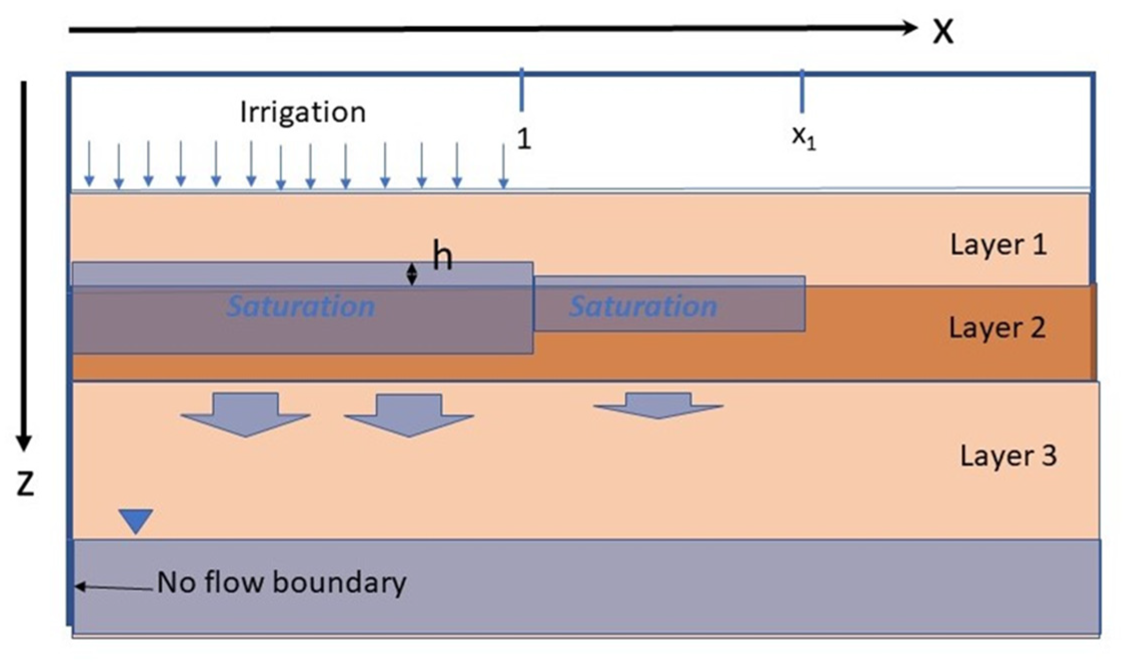
The conceptual model for this paper is similar to Ref. [18] and is shown in Figure 1. There are three semi-infinite layers of homogeneous soils, in which the second layer is of lower permeability. The left boundary condition is a no flow boundary, i.e., this is a line of symmetry and conditions to the left reflect those on the right. The upper boundary is the base of the agronomic zone, the left side of which underlies irrigated agriculture, and to the right side underlies non-irrigated agriculture. The upper boundary condition is a with a downward water flux, irrigation accession, as determined by agricultural practices, including channel leakage and spillage. For the one-dimensional systems discussed below, the whole upper surface is irrigated. The lower boundary condition is the water table, which is assumed to be constant.
The layers of the unsaturated zone have been parameterised using a modified Mualem–Brooks–Corey model of soil hydraulic properties for each layer [20,21]. The water retention curve is given by:
where ψ is the soil suction, hb is the air-entry point, λ is a fitting parameter, and the relative saturation, Θ, is given by
Θ = 1, ψ ≤ hb
The relative permeability, Kr, is given by:
where m is a fitting parameter related to the connectivity of soil pores.
Kr = Θm
The hydraulic conductivity, K, is obtained by multiplying Kr by the saturated hydraulic conductivity. These parameters will be different for the different layers and a subscript i will be subsequently used to distinguish layer i. The parameters are assumed to be the same for both vertical and horizontal properties, except for the saturated conductivity. A superscript h and v will be used with the saturated hydraulic conductivity to characterise anisotropy. The values given to the parameters is given in the Methods section.
The underlying equations are non-dimensionalised using the vertical length scale, l2, timescale S2 l2/Ks2v, horizontal length scale x0; where li is the thickness of the ith layer; x0 is the half-width of the irrigated area; Ksiv is the saturated vertical conductivity of the ith layer; and S2 is the specific yield for the second layer for the initial dry conditions. The purpose of the non-dimensionalisation is to simplify as much as possible using scaling and non-dimensional variables.
2.2. Modelling Individual Actions
In this section, the theory for recharge response to a reduction in irrigation accession is developed. The system is assumed to be initially in equilibrium and the change in irrigation accession occurs at time zero. The theory is adapted from the kinematic wave model [10] in which the initial and final states are unsaturated zone and processes are one-dimensional (vertical). This is described in Section 2.2.1. In Section 2.2.2, this theory is adapted to situations, in which the initial state is perched. For perched water tables, water can move laterally from the irrigation district and process can be two-dimensional. Under certain conditions, these two-dimensional processes can be reasonably represented by one-dimensional processes, for which the modelling is simpler.
2.2.1. Kinematic Wave Theory for Unsaturated Zones
Where the original irrigation accession is sufficiently small, the soil zone is initially unsaturated for all layers. In the application of the kinematic wave approach [10] to the above conceptual model, the reduction in irrigation accession at the top of layer one causes the moisture content and soil potential there to reduce to the value for which the intrinsic vertical hydraulic conductivity, Kr1, equals the new non-dimensional irrigation accession flux, A. The kinematic value approach follows how any particular value of vertical hydraulic flux (and associated moisture content and soil potential) between the old and new irrigation accession fluxes travels through layer one. The higher value of flux (and associated moisture content and soil potential) travels more quickly, with the fastest being that for the old irrigation accession and the slowest being that for the new irrigation accession. When the fastest value reaches a particular depth, the flux at that depth begins to gradually reduce from the old irrigation accession until the slowest value reaches that depth and flux stabilizes at the new value. Any value of flux can be followed through the three layers to the water table. The theory implies that the speed of any value in the ith layer is given by:
where z is the non-dimensional depth of the soil potential below the land surface, and θ is the moisture content, θ; in that layer that corresponds to the soil potential; and:
Gi = mi Si Ksiv/Ks2v
Recharge will remain at the old value until the fastest value reaches the water table and reduce until the slowest value reaches there and will then stabilize at the new value. The recharge between these values can be obtained by interpolating the times for other values to reach the water table.
Should there be any further measures that reduces irrigation accession, then the above steps can be repeated. Since the group velocity for these new values are lower, there should be no interference between the steps.
2.2.2. Soil Zone Initially with Perched Water
In this section, we consider the situation for which there is a perched water table at the base of the first layer but does not intercept the upper surface of layer 1 and this remains so throughout the transition from old accession rate to new accession rate. It will be shown in this section that most state variables of interest will move exponentially from the old equilibrium value to the new equilibrium value.
If layer one is sufficiently thick, equilibrium conditions can be reached in which the infiltration through the clay equals that of the irrigation accession [18]. The non-dimensional thickness of the perched water above the second layer, heq, under equilibrium conditions is given by:
where A is the non-dimensional irrigation accession; B and φ are dimensionless variables, defined by:
and the integral in Equation (10) is from hb to ∞ and φ is assumed to be insensitive to A.
heq = (A − 1 − φ)/(1 + sqrt(B))
B = Ks1h l22/(Ks2v x02)
φ = (A − 1) ∫ dψ/((A/Kr2v (ψ) − 1 ) l2)
Perching only occurs if
and does not intercept the upper boundary condition if
A > 1 + φ
l1/l2 > (A − 1 − φ)/(1 + sqrt(B))
Under conditions of quasi-steady state perched water, and a perched water of zero thickness under non-irrigated agriculture in the fringes of the irrigation areas, the transient condition is given by [18]:
where β is the ratio of s1 to S2; and s1 is the specific yield of layer 1 after wetting front has already passed through. This has the solution:
where heq and h0 are respectively the new equilibrium head and the old equilibrium head. This shows that perched head reduces exponentially to the new equilibrium conditions. The effect of two-dimensional flow is indicated by the dimensionless parameter B, where B = 0 corresponds to one-dimensional flow and large B corresponds to significant lateral movement. The effect of B is to not only reduce the steady-state ponded head, but to also quicken the rate at which the new equilibrium is attained. To understand this better, we consider the dimensioned time scale in the exponential function:
h = heq + exp( − t (1 + sqrt(B))/β) (h0 − heq)
ts = l2 S2 β/((1 + sqrt(B)) Ks2v)
As B becomes very large, ts becomes in dimensioned variables:
ts~x0s1/sqrt(Ks1hKs2v)
Hence, the time scale involves a mixture of the horizontal conductivity of the sand layer and the vertical conductivity of the clay layer. This is not surprising given that these soil parameters influence both the magnitude of the ponded head and the ability of the water to move laterally. In parallel with the ponded head increasing exponentially to the equilibrium value, the vertical flux through the second layer under the irrigated agriculture would also approach the equilibrium value, qeq:
where q0 is the vertical flux at initial equilibrium and is related to h0 by:
q(t) = qeq − (qeq − q0 ) exp( − (t − t0) (1 + sqrt(B))/β)
q0 = 1 + h0 + φ
There is a similar relationship between qeq and heq .The extent of the wetting outside of the irrigation field, x1, also decreases exponentially under the assumptions used from the original equilibrium value, x10, to the new equilibrium value, x1eq, in parallel with the ponded head.
where x10 is related to h0 by:
x1(t) = x1eq − (x1eq − x10) exp( − (t − t0) (1 + sqrt(B))/β)
x10 = h0 sqrt(B) + 1
However, the aggregated vertical flux through the clay external to the irrigation field is no longer proportional to the extent of wetting, as areas that had wetted previously will continue to drain. This additional term is ignored in the current modelling.
2.2.3. Change from Perched Water Table to None
If the new irrigation accession is such that A < 1 + φ, there is no perched water in the new equilibrium situation. The solution to Equation (12) in that situation is still given by Equation (13), but with the term heq substituted by (A − 1 − φ)/(1 + sqrt(B)). This allows the time for the perched head to go to zero to be estimated. After that time, layers 2 and 3 begin to drain; and Equations (5) and (6) apply.
2.2.4. Initial State with Rejected Recharge
For the situation where the head of the perched water under the irrigated agriculture intersects the upper boundary (i.e., the first layer is saturated under irrigation), Equation (11) no longer applies and some of the irrigation accession is returned to the surface as there is no opportunity of any further infiltration. We refer to this situation as rejected recharge. If this is the starting situation, then a minor reduction in the irrigation accession may have no effect on recharge, but rather the volume of rejected recharge is reduced. It is only when the irrigation accession is reduced sufficiently for Equation (12) to hold that recharge will change in response to the reduced irrigation accession. The volume of rejected recharge should reduce to zero almost immediately and the head of perched water will also begin to respond immediately. The Equations (12), (13), (16) and (18) should then apply.
2.3. Modelling of Multiple Actions
In Section 2.2.1, the theory for a soil zone with no perched water showed that the response of successive actions, which reduced irrigation accession, were independent of each other. This is unchanged for perched water tables. As can be seen in Equation (12), where it does not matter if the initial condition is an equilibrium situation. The value of the head at the time of the water use efficiency change is used for h0. Taken together, the methodology across the range of situations described in Section 2.2.1, Section 2.2.2, Section 2.2.3 and Section 2.2.4 does not change under multiple actions, which reduce irrigation accession.
For the first irrigation water use efficiency improvement following a new development, the soil zone may not have come to a hydraulic equilibrium at the time this improvement occurs. Two situations are considered: (1) the wetting front has reached the water table, but perched water has not equilibrated and (2) wetting front is in layer three when new measure occurs.
In the first situation, the effect of reduced irrigation accession should almost be immediate. The perched head should move exponentially to the new equilibrium value or zero (if the new equilibrium state has no perched water). The flux through the second layer should change exponentially in response and the system behaves as in Section 2.2.2. The change in flux will then cause a change in recharge when the pressure effect reaches the water table. Where there is no perched water in the new equilibrium state, layers two and three begin to drain
In situation (2), the perched head will still respond exponentially, as will the flux through layer two. There is some chance that the pressure effect of this may reach the wetting front before it reaches the water table, causing a slight modification in the change in flux at the wetting front and the speed at which it moves. Once the wetting front has reached the water table, the system will respond as per Section 2.2.2.
2.4. Transfer Function and Superposition
Section 2.3 contributes to the second objectives; namely developing a way to implement transfer functions for the estimation of recharge from irrigation areas at district-wide scales. More specifically, it defines modified transfer functions for which superposition may apply. It also develops the theory for the linear reservoir model, in a way that is relevant to irrigation systems with perched water.
A transfer function is a mathematical model of a system that maps its input to its output (or response). A normalised transfer function TF(t) is normally defined as:
TF(t) = (R(t) − Ro)/(IAn − IAo)
An analogous transfer function can be defined for drainage volumes (D(t)). These transfer functions will mostly be used for displaying results in Section 4. Where there is no rejected recharge, TF(t) = 0 for t = 0; and approaches 1 for large times. Hence, it represents a cumulative probability distribution for time delays for pressure to travel through the vadose zone. Where there is rejected recharge, TF(t) is less than one for large times but the sum of transfer functions for recharge and drainage approaches one.
As the system is not necessarily linear, there is no reason to believe that superposition would necessarily apply to a range of situations. Some situations are not expected to follow superposition include those where thresholds are involved, such as the initiation of perching or rejected recharge. The addition of two actions, that do not meet individually exceed the threshold, but in aggregation do so, is not linear. The transfer functions, as defined in Equation (20), is clearly not appropriate for superposition, because of the threshold where rejected recharge occurs. For the purpose of superposition, a modified transfer function for the recharge is defined:
where the superscript * indicates the minimum of irrigation accession (IA) and the maximum irrigation accession without rejected recharge. We can define a similar transfer function for drainage, TF’’, where
where Do is the original drainage rate, IA** is the maximum of IA and the maximum irrigation accession that occurs without rejected recharge.
TF’(t) = (R(t) − Ro)/(IAn* − IAo*)
TF’’(t) = (D(t) − Do)/(IAn** − IAo**)
If superposition does apply, the aggregate transfer function for a sequence of actions that affect irrigation accession:
where IAj is a sequence of modified irrigation accessions that occur from j = 0 to j = p + 1 and TF’j+1 is the modified transfer function that applies for a change of irrigation accession from IA*j to IA*j+1.
TF’(t) = ( ∑j (IA*j+1 − IA*j) TF’j+1)/(IA*p+1 − IA*0)
The pattern of the aggregate TF’ with time would broadly follow that of IA, but with (a) time delays; (b) “smearing” and (c) capping at the maximum irrigation accession for which there is no rejected recharge. Where superposition applies, this would simplify the numerical process by generating the transfer function for the combination of actions from the transfer function of individual actions.
Within the parameter range used, superposition provided a reasonable approximation to new developments because of the lack of hydraulic interaction between developments [18] i.e., spatial superposition. In this paper, we will test the principle of superposition for a set of actions acting on the one irrigation development at different times, i.e., temporal superposition. For the modelling in this paper, a new development is assumed to be followed by a succession of water use efficiency improvements.
2.5. Theory for the Linear Reservoir Model
The transfer functions for application in Equation (23) can be generated from PerTy3, using the methodology described in Section 2.1. However, one of the objectives of the paper is to explore the application of conceptual models for the transfer function and, in particular, the linear reservoir model. The separation between physically based and conceptual models is not black and white. While the theory above describes physical processes, the analytical model is simplified, with assumptions such as spatial homogeneity, flat surface elevations etc. It is possible to consider transfer functions as conceptual models, using enough complexity to broadly replicate the recharge response. Such models have previously been used for recharge [6,10].
The physical processes above are consistent with a linear reservoir, for which the inputs, IA, and outputs, R, are related through the storage, M:
where M is the total amount of water in the unsaturated zone, including the perched water table and IA* is the irrigation accession, adjusted for rejected recharge, if it occurs. If R is linear with respect to M i.e.,
dM/dt = IA* − q
q = cM + d
This leads to M being exponential with respect to time with coefficient −c. There is a time lag between q and R due to the time for pressure fronts to move through the unsaturated zone. This leads to:
where Δ represents the change in the parameter, and c, t5 and t6 become fitted parameters. While the theory in previous sections give physical meaning to parameters c and tl or fitted to model outputs, they can be also fitted to groundwater responses.
Δ R = Δ IA (1 − exp(− c (t – t5))), t > t6
The exponential nature of the linear reservoir function is similar to that of many of the parameters in PerTy3. This is perhaps not surprising, given that the mass balance Equation (24) bears striking similarity to Equation (12).
2.6. Criteria for Rejected Recharge
Rejected recharge occurs when Equation (11) is not satisfied. The criterion for rejected recharge can be written in dimensioned form:
IA > Ks2v (1 + φ + l1/l2 + sqrt(Ks1h/Ks2v) l1/x0)
Equation (22) separates soil-related parameters (right-hand side) from irrigation accession (left hand side). This aids the parameterization of the transfer function, as over time, irrigation accession will change and gradually decrease. For many areas, rejected recharge will require drainage of some form for agriculture to be sustained. The presence or absence of drainage and the drainage volume for different irrigation accessions and different soils to calibrate the parameters in the transfer function. Where Equation (23) applies, the drainage volume, D, can be written as:
where data for drainage volumes exist, they can also be used for calibration.
D = IA − Ks2v (1 + φ + l1/l2 + sqrt(Ks1h/Ks2v) l1/x0)
3. Methods
This section describes the methodology to meet the objectives of the paper. Section 3.1 provides a description of the modelling experiments used to address objectives 1 and 2. In particular, the experiments contribute to 1(a) testing the theory and the model by comparison with a numerical model; 1(b) implementing the model for the irrigation whole-of-life; 2(a) trialling the principle of superposition of recharge models in response to individual actions over the irrigation whole-of-life; and 2(b) seeking simple conceptual models that can approximate the recharge distribution for individual actions and in particular the linear reservoir model.
Section 3.2 and Section 3.3 describe modelling experiments that contribute to objective 2; namely:
- trialling the principle of superposition of recharge models in response to individual actions over the irrigation whole-of-life; and
- seeking simple conceptual models that can approximate the recharge distribution for individual actions and in particular the linear reservoir model.
Section 3.4 and Section 3.5 contribute to objective 3 by providing information to support the calibration of integrated models for application to scenario modelling.
3.1. Modelling Experiments
A series of modelling experiments have been conducted to achieve objectives 1 and 2. The models are partitioned into one-dimensional (1D) modelling or two-dimensional (2D) modelling. For the 1D modelling, the variable B has effectively been set to zero. For numerical models, the whole of the upper surface is irrigated and the right-hand boundary has zero lateral flux of water. The degree to which lateral transport is important for the 2D modelling is dependent on the parameter B. This has been set to one for this paper.
Either (or both) the PerTy3 and numerical models have been used. The PerTy3 semi-analytical model has been designed to satisfy the above theory. This does not use a mesh, but rather is designed to estimate time delays. Fluxes are generally estimated at annual time-steps. For transmission of pressure through the unsaturated zone, the time delays are estimated for steps in soil suction and then interpolated to provide recharge at annual time-steps.
The numerical modelling is undertaken using FEFLOWTM [22]. FEFLOW is an acronym of Finite Element subsurface FLOW simulation system and solves the governing flow equations in porous media for variable saturation. Richards’ equation is solved for a single dominant fluid phase (in this case water) with an assumed stagnant air phase that is at atmospheric pressure everywhere. FEFLOW implements a number of empirical and spline models for variable saturation and in this work the empirical Mualem–Brooks–Corey model is used [20,21]. Fine mesh refinement is used to achieve stable numerical solutions for the adopted choices of the Mualem–Brooks–Corey model parameters. The set-up for both 1D and 2D modelling is shown in Figure 2. For the 1D modelling (Figure 2a), the third layer has a thickness of 15 m, while for the 2D modelling, it has a thickness of 5 m. The vertical mesh size for both is 10 cm (250 (1D) or 150 (2D) elements), while for the 2D modelling, the horizontal mesh size is 10 m (200 elements).
The models have mostly been parameterized using values relevant to the Mallee region of Southeastern Australia [23]. These default values are shown in Table 1. In addition to the parameters in the Tables, the following default values were used:
- irrigation half-width, x0, 500 m for 2D modelling;
- dimensionless parameter B: 0001 (1D); 1 (2D); and
- pre-irrigation accession for new development: 10 mm/year.
Table 2 lists the modelling experiments, with non-default parameters and whether the semi-analytical and/or numerical model is used. These modelling experiments can be categorized as follows:
- (i)
- Experiments 7 (1d) and 8 (1D) model the transient behaviour from an equilibrium state to a new equilibrium state in response to a single reduction in irrigation accession. The modelling outputs of PerTy3 and FEFLOW will be compared. In addition, outputs will be used in Section 3.2 and Section 3.3 to test superposition and find approximants for the linear reservoir model.
- (ii)
- Experiments 9 (1D) and 14-1 (2D) model the transient behaviour from an equilibrium state to a new equilibrium state in response to multiple water use efficiency improvements. This includes the behaviour of the perched head and for the 2D modelling recharge under the external to the irrigated agriculture. The modelling outputs of PerTy3 and FEFLOW will be compared. The outputs of the two models will be compared to show differences between 1D and 2D situations. Moreover, the outputs will be used in Section 3.2 and Section 3.3 to test superposition, including superposition of approximants.
- (iii)
- Experiments 10 (1D) and 15 (2D) model the transient response from an equilibrium pre-irrigation state to a new equilibrium in response to irrigation development and successive irrigation efficiency improvements. Only PerTy3 is used. The modelling outputs are used to in Section 3.2 to test superposition. The outputs for 10a and 15a come from [18].
- (iv)
- Experiment 11 (1D) models the sensitivity of the recharge over time for the irrigation whole-of-life to Ks2v. The values of Ks2v are chosen so that soil zone goes from no perching to perching for almost the entire modelling period.
3.2. Superposition Experiments
There are three superposition experiments:
- The first is for a series of water use efficiency improvements, using outputs from experiments 7, 8 and 9. The modelling experiment 9 represents a combination of water use efficiency changes of 230 to 100 mm/year and 100 to 50 mm/year, separated by 5 years. The numerical outputs for experiments 7 and 8, which each represent the individual transitions, but with each starting from an equilibrium state, were superimposed, using Equation (21). This superposition is compared to the semi-analytical and numerical modelling outputs for experiment 9.
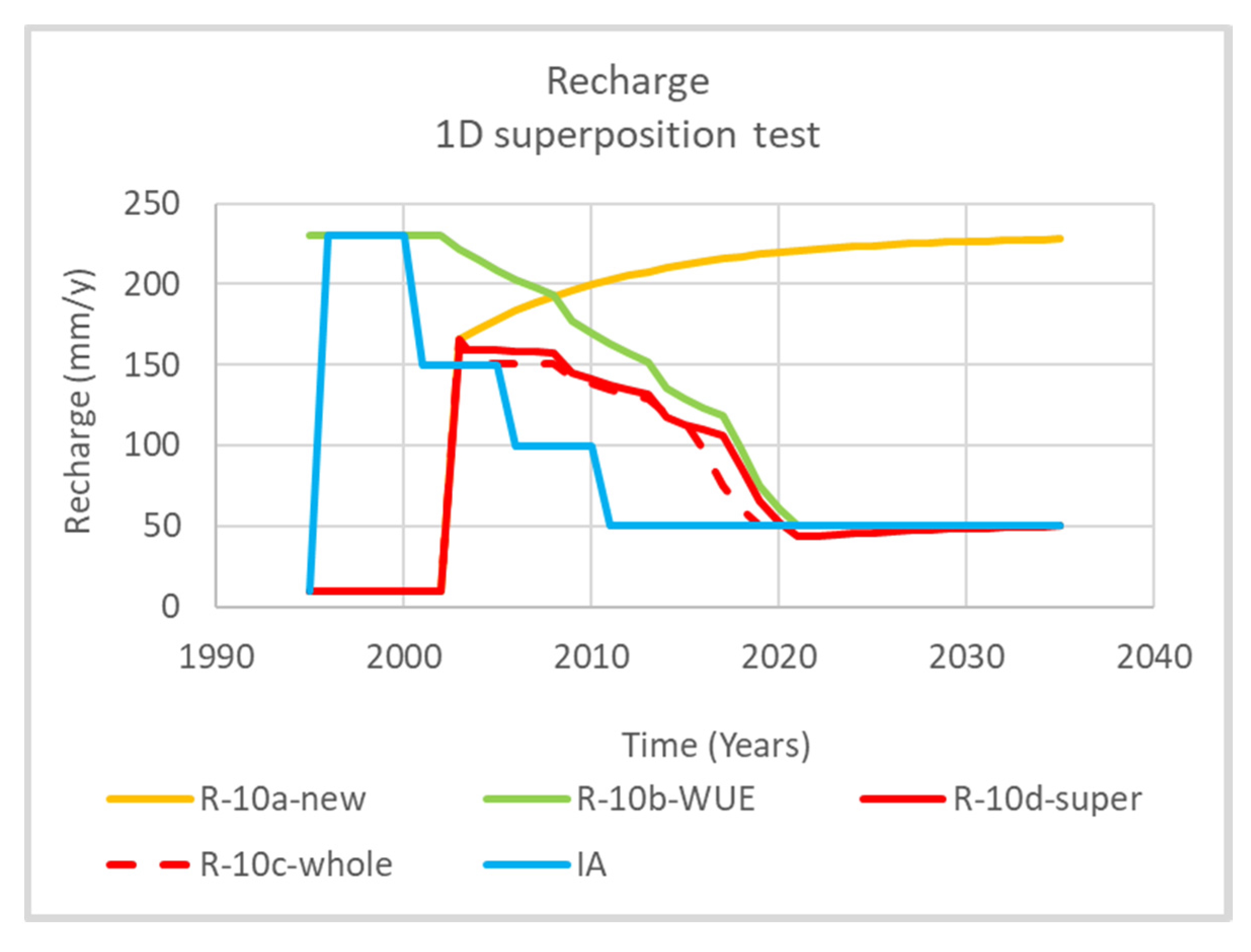
- The second experiment (Experiment 10 (1D)) is for a one-dimensional irrigation whole-of-life i.e., a new development followed by a succession of water use efficiency improvements. The PerTy3 model is implemented for three 1D scenarios: 10a a new development that started in 1996; 10b is a sequence of water use measures separated by 5 years, starting in 2001 (the 1996s state of a new development starting in 1921 approximates an initial equilibrium state); and 10c, the same sequence of water use measures following a new development in 1976. The superposition of 10a and 10b (10d) is compared with 10c.
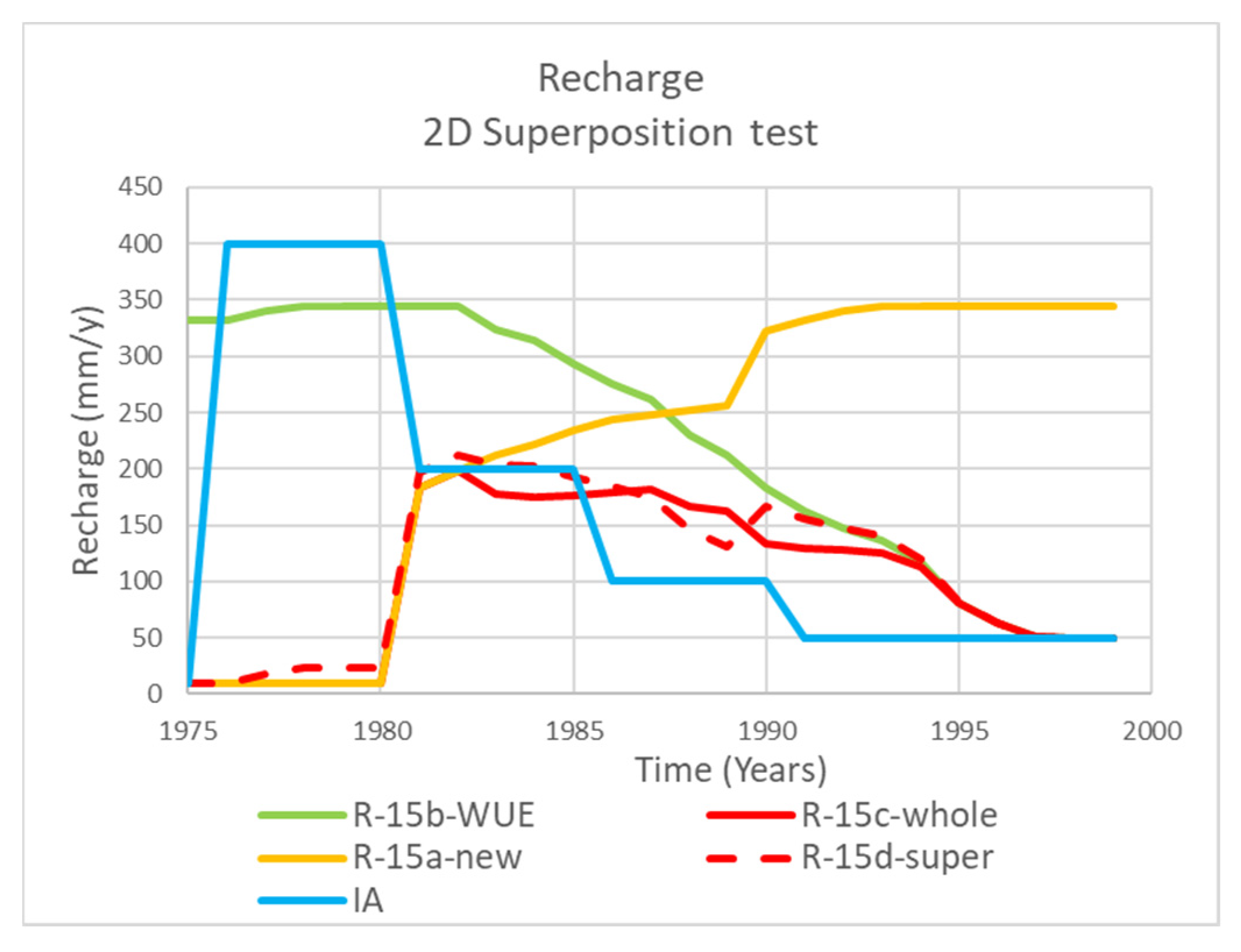
- The third experiment (Experiment 15(2D)) is for a two-dimensional irrigation whole-of-life. The PerTy3 model is implemented for three 2D scenarios: 15a, a new development starting in 1976; 15b, a sequence of water use measure separated by 5 years and beginning in 1981 (the 1981 state of a new development in 1961 approximates an initial equilibrium state); and 15c, the same sequence of water use measures following a new development in 1976. The superposition of 15a and 15b (15d) is compared with 10c.
The superposition of spatially separate new developments has been previously tested [18]. Water use efficiency measures in separate developments would be expected to be a weaker test of superposition and is not tested further here.
3.3. Seeking Approximants
Approximants are fitted to the FEFLOW transfer function outputs for modelling experiments 7 (1D) and 8 (1D) using Equation (26).
Moreover, the superposition of the approximants for a series of water use efficiency improvements is tested by comparing to the FEFLOW output for the transfer function for modelling Experiment 14-1.
3.4. Using Drainage Outputs for Calibration
Drainage volumes can be potentially used to calibrate the PerTy3 model. To test this, drainage and soil data are obtained for the Loxton–Bookpurnong irrigation district in the Mallee region.
The soils of the district are categorised into six types. The 3a soils are those for which sub-surface drainage was required, while the 3b soils, none was required. The 3b soils are further divided based on sub-surface characteristics and 3a into two for the different irrigation districts.
Drainage volumes have been measured for the Loxton region [24,25], but not for the Bookpurnong area. For the latter, the presence or absence of sub-surface drainage was noted. The drainage volumes and estimated irrigation accessions [24] were averaged for four periods (1970–1990, 1990–2002, 2002–2006, 2006–2013). These four periods correspond to periods with different estimated water use efficiency factors [24]. The period before 1970 is largely ignored, as a comprehensive drainage scheme was not available before this time. Drainage was only assumed to occur for 3a soils.
Table 3 summarises the soil and drainage characteristics for the six soil types. Areas with no drainage for a period are denoted N/D; areas for which the drainage volume is known; while those where drainage occurs but the volume is unknown are denoted D.
To calibrate PerTy3, Equations (27) and (28) are first applied to create contours of drainage volumes using Ks1h and Ks2v as variables, keeping other variables constant. By varying Ks1h and Ks2v are then varied to best fit the drainage data in Table 3. One way to constrain non-uniqueness is to have the same values for all 3a soils and another one for all 3b soils.
3.5. Whole-of-Life Modelling
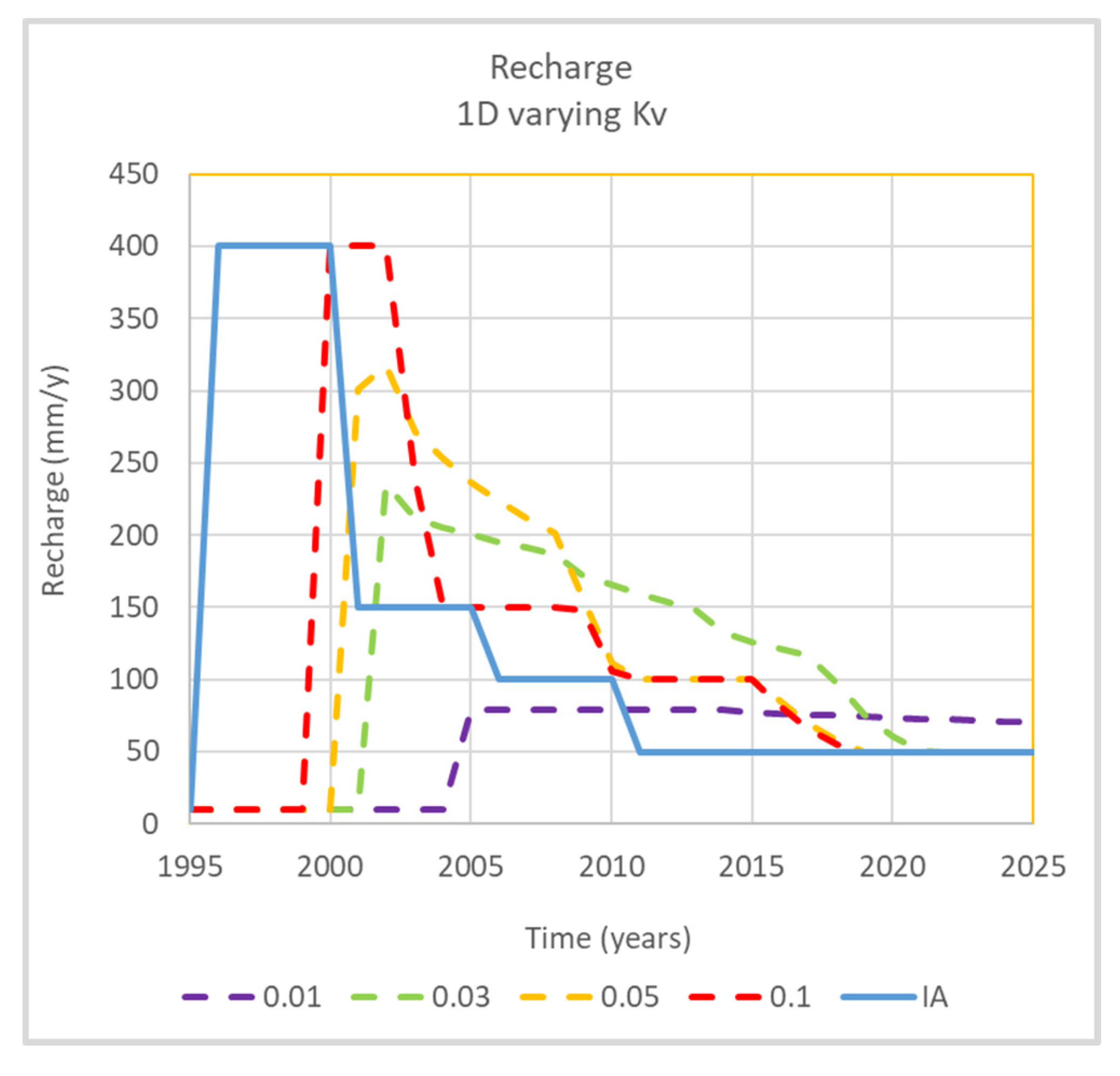
The modelling experiment 11(1D) aims to show the sensitivity of the irrigation whole-of-life recharge to Ks2v. The PerTy3 model is implemented with the following values for Ks2v: (a) 0.1 (b) 0.05 (c) 0.03 (d) 0.01 cm/day. The perching conditions show the full range of behaviour over this range of Ks2v: The irrigation accession is varied from 10 to 400 to 150 to 100 to 50 mm/year, separated by 5 years. This should provide some insight on the interaction between IA and Ks2v and whether the groundwater response may be able to be used to calibrate soil parameters.
4. Results
4.1. 1D and 2D Modelling
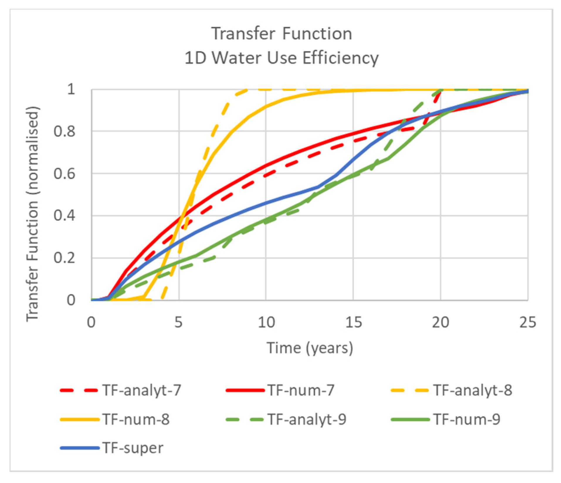
Figure 3 shows the 1D modelling outputs for the transfer function for Experiments 7, 8 and 9. The transfer functions outputs from FEFLOW and PerTy3 models generally match well for both 7 and 8. The worst comparison is for Experiment 8 (non-perching), where the numerical result shows greater “dispersion” of recharge.
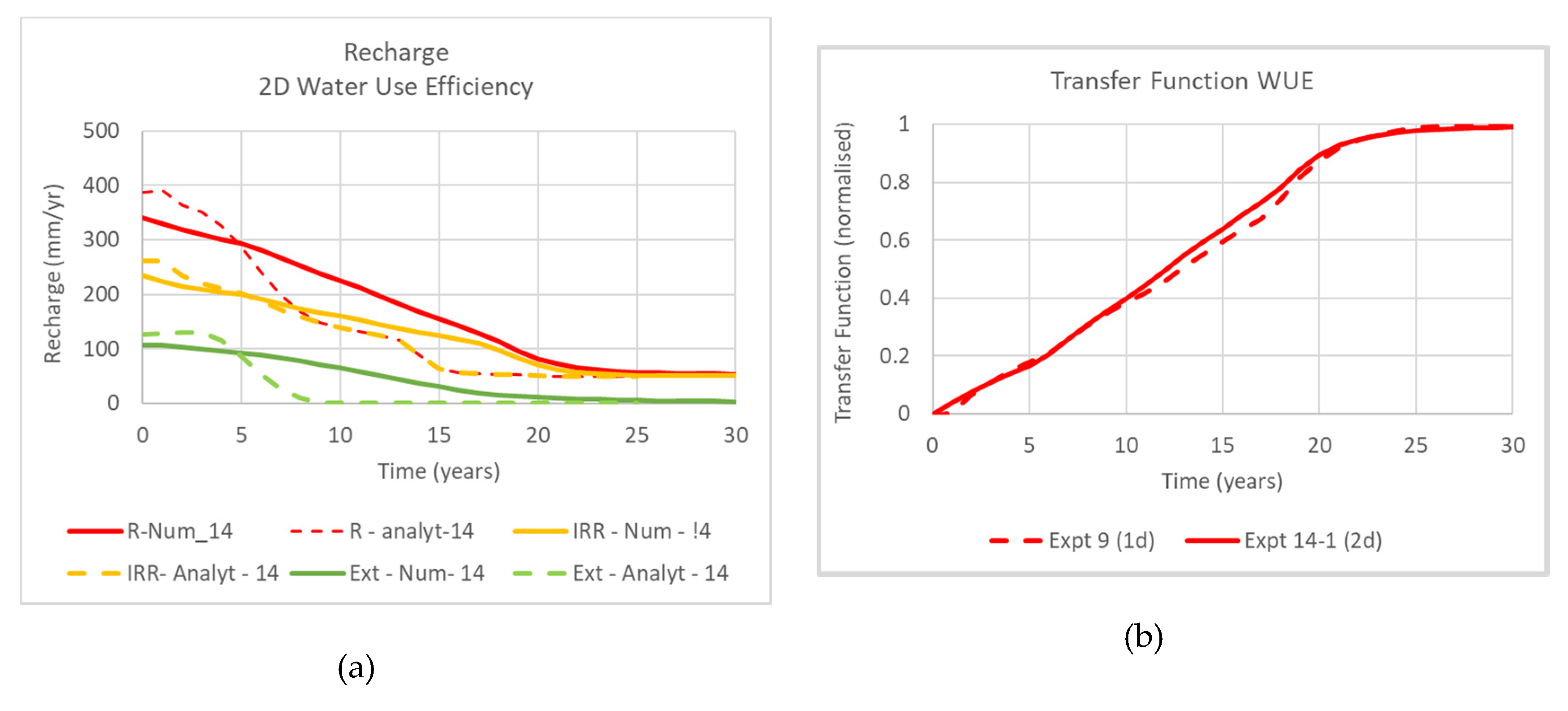
Figure 4a shows that for 2D modelling, there is a greater discrepancy between the outputs of FEFLOW and PerTy3. The partitioning between the recharge under irrigated agriculture and external to irrigated agriculture is initially consistent between the two models. However, the recharge for the area external to irrigation is predicted by PerTy3 to decline in about 8 years, compared to 20 years for FEFLOW. Similarly, PerTy3 predicts the recharge under the irrigated agriculture to decline within 15 years compared to 22 years for FEFLOW. The total recharge for both models declines at similar rates to that under the irrigated agriculture.
Figure 4b shows that the transfer function from the 2D modelling (Experiment 14-1) is almost identical to the that from the 1D modelling (Experiment 9), despite there being a reasonably even split of recharge both under and external to the irrigated agriculture. Moreover, the irrigation accession required for rejected recharge is significantly greater for the 1D situation. There does not appear to be the sensitivity of the exponential time scale as shown in Equation (14).
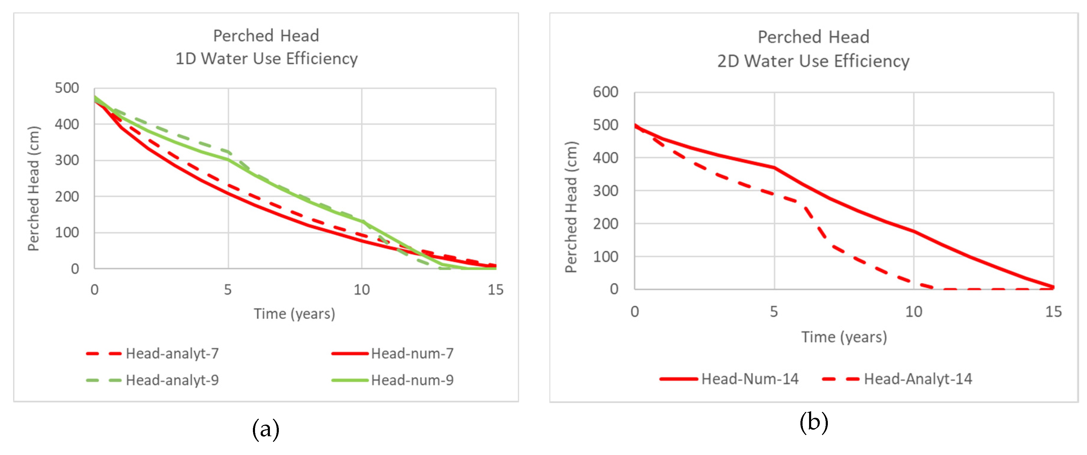
Figure 5 shows the modelled perched head for both 1D and 2D situations. Again, the outputs are consistent for the 1D situation, while there is a significant discrepancy for the 2D modelling. The perched head is initially consistent, but for the 2D situation, the semi-analytical modelled perched head declines in only 10 years compared to 15 years for the numerical model. This difference might explain that for the recharge in Figure 4. Moreover, the decline in the numerical output is piecewise linear, while that in the semi-analytical model piecewise exponential.
4.2. Superposition Experiments
Figure 6 shows the transfer function for the superposition of modelling Experiments 7 and 8 and compares this for both the FEFLOW and PerTy3 model outputs for Experiment 9. While the superposition is higher than either of the outputs for Experiment 9, the shape and time scale of recharge reduction is similar.
Figure 6 shows the results of the superposition Experiment 10. It shows the modelled response to the new development and for the subsequent water use efficiency improvements. The superposition (solid red) resembles the modelled output (red dashed). The resultant pattern is a smoothed and delayed version of the irrigation accession (shown in blue). The irrigation accession is the input to the model and reflects initially the pre-irrigation conditions, then the irrigation history from 1976 to 2010 and then the assumed final irrigation accession of 50 mm/year from 2010 onwards.
Figure 7 shows the results of the superposition experiment 15. Again, the superposition (red dashed) matches the modelled recharge (red solid) and the resultant form is a smoothed and delayed version of the irrigation accession (blue). The irrigation accession reflects the irrigation history from pre-irrigation rate of 10 mm/year, development in 1976 and irrigation improvements from 1981 to 1991 and then the final assumed rate of 50 mm/year.
4.3. Use of Drainage Data to Calibrate the Transfer Function
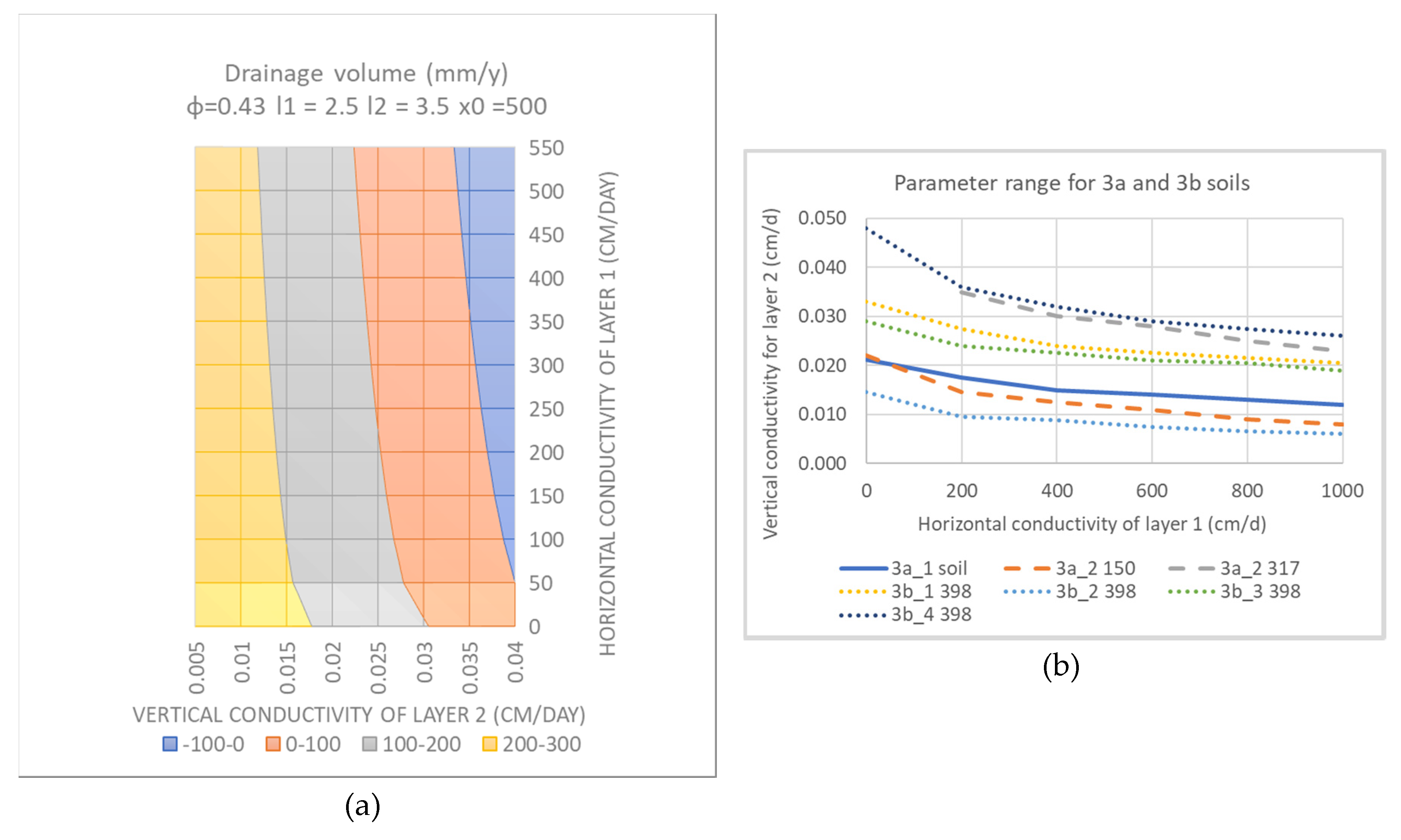
Figure 8a shows contours of drainage volumes (mm/year) for the 3a_1 soil for the Loxton–Bookpurnong District for an irrigation accession rate of 339 mm/year, based on soil hydraulic properties. Negative values mean that there is no drainage. For this value of IA, the drainage has been estimated to be 173 mm/year. This implies that the soil properties follow a contour, beginning with Ks1h = 0 and Ks2v = 0.0212 cm/day. The drainage volumes for other values of IA in Table 3 leads to the same contour. The relationship between the two conductivities for this contour is shown as a solid line in Figure 8b.
While the presence or absence of drainage is known for soil 3a_2, the drainage volumes are not. This knowledge provides some constraints on the soil properties. The absence of drainage for a value of IA of 150 mm/year, but drainage at 317 mm/year means that the soil properties lie between the two dashed contours in Figure 8b. If we are seeking one set of soil properties denoted as 3a, the contour found for 3a_1 would be consistent with this constraint for all but the lowest value of horizontal conductivity.
For 3b soils, there is no drainage, even for a value of IA of 398 mm/year. This means that the soil properties must lie above the dotted contours in Figure 8b. If we are seeking a single set of soil properties for all 3b soils, the strongest constraint is given by 3b_4. This implies that Ks2v > 0.025 cm/day for high values of Ks1h or >0.045 cm/day (low values of Ks1h ). Soil properties can then only be further constrained by fitting to the groundwater response.
4.4. Approximants
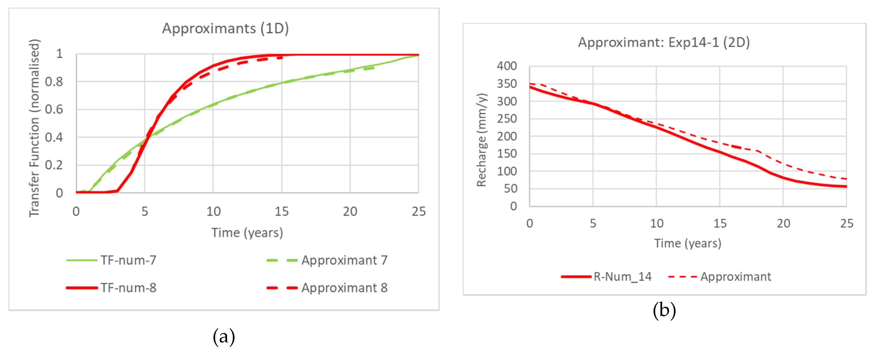
Figure 9a shows fitted approximants for the transfer functions for FEFLOW outputs for experiments 7 and 8 (1D). The exponential functions with a time delay were reasonable approximations for both the perched situation and the unperched situation. For the latter, the approximant underestimated the later stages.
Figure 9b showed the superposition of these approximants for a series of successive reductions of irrigation accession from 350 to 200 to 150 to 100 to 50 mm/year at time intervals of 5 years. The superposition of the approximants overestimated recharge during the later stage, but still provided a reasonable approximation for application to groundwater modelling.
4.5. Whole-of-Life Modelling
Figure 10 shows the recharge response to a whole-of-lifetime sequence for irrigation areas. The results show that time delays for new developments increase for decreasing Ks2v. The highest value of Ks2v (01.1 mm/day) produces the earliest and highest peak value, equalling IA after five years. For other values of Ks2v, the peak values occur later and have lower values, with the lowest value of Ks2v (0.01 mm/day) having a barely discernible peak. For Ks2v = 0.1 mm/day, the shape mirror that of IA, but with a delay varying from 3 to 8 years. For the next highest value of Ks2v, 0.05 mm/day, recharge reduces exponentially until there is no perched head and then falls to match the recharge for 0.1 mm/day. For the third highest value of Ks2v, 0.03 mm/day, recharge also falls, more or less, exponentially (but more slowly than for Ks2v = 0.05 mm/day), to where the perched water disappears and then falls to the final value only two years after the previous curves, and with a time delay of up to twelve years after IA. Reduction of Ks2v and the presence of perched water leads to lower peak recharge values, greater time delays. When perched water disappears, the difference between the recharge disappears.
5. Discussion
This paper has built upon a semi-analytical model, PerTy3, to estimate the impact of reduced irrigation accessions on recharge, adapting an analytical model [10]. This has focused on deep vadose zones, where time delays for pressure transmission can be significant and where perching can occur. The theory allows straightforward changes in the status of perching as irrigation accession increases after development and reduces after infrastructure and water use measures. In addition, the theory has been generalized to two-dimensional situations. The use of non-dimensional parameters A and B reflect these transitions, A for perching and B for lateral flow. Perching will occur where A is greater than 1 + φ and rejected recharge occurs where A is large enough for criterion (Equation (11)) to no longer hold. One-dimensional behaviour will occur when B is small and lateral movement becomes significant as B becomes greater than one.
5.1. Accuracy of the Model
The model is conceptual in nature and simplifies the processes under irrigation areas. For example, topography is assumed to be flat and sub-surface soil layers are homogeneous in nature. The expectation is that some parameters will need to be calibrated, but the data to do this is limited. The aim is to capture the key processes, while keeping the model as simple as possible. Parameters related to the key processes can then be calibrated.
The testing of the model can occur in three ways:
- (1)
- model-to-model comparison;
- (2)
- comparison of assumptions with past literature; and
- (3)
- testing with field data.
Outputs from the semi-analytical and numerical models have been compared (Figure 3, Figure 4 and Figure 5). The underlying assumptions and parameters for the models are very similar. The numerical model may not necessarily be taken as a point of truth, as it may have problems with numerical instability and dispersion, especially with the fine mesh required for modelling perched water situations. From inspection, there did not appear to be issues of instability. Closer examination of results than those shown here is possible and has been conducted. The model in this paper used a more restricted set of parameters than in [18] for the new developments and so any findings needs to be qualified that they are for the range of parameters used.
The outputs for PerTy3 and FEFLOW are generally very consistent for one-dimensional situations. Even the closer inspection of outputs shows great consistency. The largest discrepancy appears to be the modelling of the drainage of unsaturated zone, where the semi-analytical model predicted a quicker response than the numerical model. However, this discrepancy occurs for drier conditions, where perching is not an issue and, hence, associated with the analytical model [10]. The most likely issue is that this kinematic wave model only considers the gravity component of Richard’s Equation and ignores the diffusive component. The latter becomes more important for drier conditions [26]. The diffusive component would lead to upward flow from the capillary fringe; thus, offsetting the gravity term and slowing the pressure fronts. This would lead to PerTy underestimating time lags for drier conditions.
The discrepancy between outputs from PerTy3 and FEFLOW is much greater for the two-dimensional modelling. The numerical modelling of total recharge is similar to the one-dimensional modelling [18], even for a value of B of 10. Figure 4b shows a similar result for reduced irrigation accessions, although the testing was limited to where B was one. The degree of similarity appears to be surprising, given the detailed processes are different. Other indicators (irrigation accession at which rejected recharge occurs and partitioning between the recharge under the irrigated agriculture are showing significant differences from 1D processes. This similarity may be useful for groundwater modelling, where the total recharge is the quantity of interest.
PerTy3 outputs shows agreement with the numerical modelling in the partition proportions and the initial response for the perched head. However, it is predicting smaller time delays overall for recharge and perched head to reduce. A possible reason for the discrepancy is the assumption that the perched head is not affecting soil infiltration external to the irrigated field. This assumption differs from some of the literature for steady-state solutions e.g., [17]. The perched head for x slightly greater than 1 should be similar to that slightly less than 1. A fall in irrigation accession would lead to not only a change in wetted area, but also a fall in the ponded head external to irrigated agriculture. Consideration of the perched head external to the irrigated agriculture would lead to behaviour closer to the one-dimensional situation.
5.2. Sensitivity and Calibration
The paper has shown how drainage volumes and the absence or presence of drainage may be used to constrain soil properties. Drainage is very sensitive to Ks2v, but much less so to Ks1h. The equilibrium perched head is also very sensitive to Ks2v, but Ks1h can significantly reduce its value. It is possible that maps of perched head could be used to constrain both model parameters. The large variation in recharge patterns in Figure 10 for reducing Ks2v suggests that groundwater responses could be used to calibrate Ks2v. Because of the spatial variability of Ks2v and the difficulty in measuring Ks2v in the field, it is difficult to provide an independent value of Ks2v within an order of magnitude, yet the impact on recharge can be very dramatic.
5.3. Superposition and Approximants
This paper describes superposition experiments in time. The transfer function for a new development in the vicinity of an existing development will be approximately the same as that far away from any existing developments for the parameters tested [18]. This paper extends on that work by showing that the change in recharge from a superposition of independent actions is almost identical to that of the same set of actions occurring successively, within the range tested. This means that it is feasible to consider the numerous actions occurring both spatially and temporally across the irrigation district could be considered as independent actions and, hence, the total recharge could be considered as a sum of the changes in recharge from the individual actions. If this is shown to be the case through further testing, this could simplify the analysis of a complex irrigation district. Because there are thresholds with perched water tables and rejected recharge, there are limitations to the range of situations that superposition applies.
In parallel to considering superposition, it may be possible to use simpler approximants for the transfer function. Figure 9a showed that simple exponential functions with a built-in time delay provided a reasonable approximation to 1D transfer functions from numerical modelling. Figure 9b showed that the superposition of these approximants provided a reasonable approximation to modelling experiment 14-1. The delayed exponential function is consistent with linear reservoir modelling used by others for the vadose zone [6]. The modelling shows that there is some potential to use simple additions of transfer functions for individual actions. The fitted exponential decay parameter is strongly related to the vertical conductivity of the impeding layer.
5.4. Learnings from the Modelling
The modelling outputs has shown that the effect of a low conductivity layer is to lengthen time delays between changes in irrigation accession and recharge, perhaps up to fifteen years for the parameters considered here. This has implications for salinity management, as this implies that groundwater pumping or other engineering works may need to be maintained until the impacts of the water use efficiency measures are effective. Where groundwater is fresh, the delays in reduction in irrigation returns to the river from water use efficiency measures may be large. Where decommissioning is being implemented, the time delays are expected to be much longer again.
In summary, there has been significant progress towards efficient modelling of recharge from irrigation areas, especially where the vadose zone is deep and where perched water tables exist. However, the following issues would benefit from more work:
- The 2D modelling for both new developments and water use efficiency measures: while the current modelling does capture some aspects consistently with the numerical modelling, it underestimates the overall time delays between a change in IA and a change in recharge.
- Drainage from unsaturated soils: The current model underestimates the time for drainage to occur from an unsaturated soil.
- Testing of superposition and approximants: The work so far shows that superposition and simple approximants has promise in simplifying the modelling of recharge from irrigation areas. However, it does need to be tested across a broader range of parameters and situations before regular use.
6. Conclusions
This paper describes the development of a model of recharge from an irrigation area undergoing water use efficiency changes in parallel with new development. It specifically addresses irrigation areas overlying perched water tables and deep vadose zones. This is particularly relevant to the Southwestern part of the Murray–Darling Basin in Southeastern Australia, where groundwater mounds under irrigation areas are pushing saline water into the River Murray. The impact on river salinity is being managed through a combination of groundwater interception schemes and water use efficiency measures.
The outputs from semi-analytical model, PerTy3, which has been adapted from an existing model [10], and compared to those from a numerical FEFLOW model. For the one-dimensional (1D) situation, (i.e., modelling of large irrigation areas with low horizontal hydraulic conductivity), the outputs are consistent for situations with perched water tables. Where there is rejected recharge, the recharge will not change until the irrigation accessions reduces so that there is no longer rejected recharge. In the absence of rejected recharge, the perched head (and recharge) falls exponentially in response to reduced irrigation accessions. If the reduction in irrigation accession is such that perched water tables disappear, or there were no perched water tables initially, the model is underestimating the time delays for pressure changes to move through the unsaturated zone as the soil drains.
PerTy3 also appears to underestimating time delays for two-dimensional situations. In these situations, perched water moves laterally across the impeding layer and then infiltrates. As the irrigation accession is reduced, the ponded head falls and area of wetting external to the irrigation field reduces. The 2D modelling predictions of changes in recharge from the numerical model are almost identical to those from the 1D modelling for the parameter range tested here.
The superposition of changes in recharge due to independent actions is close to the change in recharge from a succession of those actions, for the range of testing. If this applies more broadly, it may simplify the modelling of a complex irrigation area, where developments and irrigation water use efficiency measures are occurring over time and space. It also appears that simple approximations may be able to be used, which would further simplify such an analysis.
The main impact of a low conductivity layer is to delay the impact of water use efficiency changes on recharge, due to the time delays for pressure responses to reduced irrigation accession to travel through the vadose zone. This has significance for management, as the delays may mean that interim measures, such as pumping for salinity, may need to continue for longer.
Author Contributions
Conceptualization, G.R.W., D.C. and T.S.; methodology, G.R.W., T.S.; software, G.R.W., T.S.; validation, G.R.W. and T.S.; formal analysis, G.R.W.; investigation, G.R.W. and T.S.; resources, D.C., G.R.W.; data curation, G.R.W., T.S. and D.C.; writing—original draft preparation, G.R.W. writing—review and editing, D.C.; project administration, D.C.; funding acquisition, D.C. All authors have read and agreed to the published version of the manuscript.
Funding
This research was partially funded by MURRAY-DARLING BASIN AUTHORITY, project number MD004683.
Acknowledgments
The authors would like to thank the members of the Technical Committee (Juliette Woods, Ray Evans, Emmanuel Xevi and Prathapar) and Hugh Middlemis for technical advice.
Conflicts of Interest
The authors declare no conflict of interest.
References
- Perry, C. Efficient irrigation; inefficient communication; flawed recommendations. Irrig. Drain. 2007, 56, 367–378. [Google Scholar] [CrossRef]
- Wang, Q.J.; Walker, G.; Horne, A. Potential Impacts of Groundwater Sustainable Diversion Limits and Irrigation Efficiency Projects on River Flow Volume under the Murray-Darling Basin Plan: An Independent Review; Report written for the MDBA; University of Melbourne: Parkville, Australia, 2018; p. 73. Available online: https://www.mdba.gov.au/sites/default/files/pubs/Impacts-groundwater-andefficiency-programs-on-flows-October-2018.pdf (accessed on 26 March 2020).
- Yan, W.; Li, C.; Woods, J. Loxton-Bookpurnong Numerical Groundwater Model; Volume 1: Report and Figures; Technical Report DFW 2011/22; Department for Water: Adelaide, Australia, 2011. Available online: https://www.waterconnect.sa.gov.au/Content/Publications/DEW/DFW_TR_2011_22_Vol_1.pdf (accessed on 26 March 2020).
- Orr, B.R. A transient numerical simulation of perched ground-water flow at the test reactor; US Geological Survey Water-Resources Investigations Report 99–4277; Idaho National Engineering and Environmental Laboratory: Idaho Falls, ID, USA, 1999.
- Mattern, S.; Vanclooster, M. Estimating travel time of recharge water through a deep vadose zone using a transfer function model. Environ. Fluid Mech. 2010, 10, 121–135. [Google Scholar] [CrossRef]
- Wang, X.S.; Ma, M.-G.; Li, X.; Zhao, J.; Dong, P.; Zhou, J. Groundwater response to leakage of surface water through a thick vadose zone in the middle reaches area of Heihe River Basin, in China. Hydrol. Earth Syst. Sci. 2010, 14, 639–650. [Google Scholar] [CrossRef] [Green Version]
- Truex, M.J.; Oostrom, M.; Carroll, K.C.; Chronister, G.B. Perched-Water Evaluation for the Deep Vadose Zone Beneath the B, BX, and BY Tank Farms Area of the Hanford Site; Pacific Northwest National Laboratory: Richland, WA, USA, 2013.
- Rossman, N.R.; Zlotnik, V.A.; Rowe, C.M.; Szilagyi, J. Vadose zone lag time and potential 21st century climate change effects on spatially distributed groundwater recharge in the semi-arid Nebraska Sand Hills. J. Hydrol. 2014, 519, 656–669. [Google Scholar] [CrossRef] [Green Version]
- Sisson, J.B.; Ferguson, A.H.; van Genuchten, M.T. Simple method for predicting drainage from field plots. Soil Sci. Soc. Am. J. 1980, 44, 1147–1152. [Google Scholar] [CrossRef]
- Besbes, M.; De Marsily, G. From infiltration to recharge: Use of a parametric transfer function. J. Hydrol. 1984, 74, 271–293. [Google Scholar] [CrossRef]
- Schneider, A.D.; Luthin, J.N. Simulation of Groundwater mound perching in Layered Media. Trans. ASAE 1978, 21, 920–930. [Google Scholar] [CrossRef]
- Bouwer, H.M. Effect of Irrigated Agriculture on Groundwater. ASCE J. Irr. Drain. Eng. 1987, 113, 4–15. [Google Scholar] [CrossRef]
- McCray, J.E.; Nieber, J.; Poeter, E.P. Groundwater Mounding in the Vadose Zone from On-Site Wastewater Systems: Analytical and Numerical Tools. J. Hydrol. Eng. 2008, 13, 710–719. [Google Scholar] [CrossRef]
- Reid, M.E.; Dreiss, S.J. Modeling the effects of unsaturated, stratified sediments on groundwater recharge from intermittent streams. J. Hydrol. 1990, 114, 149–174. [Google Scholar] [CrossRef]
- Villeneuve, S.; Cook, P.G.; Shanafield, M.; Wood, C.; White, N. Groundwater recharge via infiltration through an ephemeral riverbed, Central Australia. J. Arid Environ. 2015, 117, 47–58. [Google Scholar] [CrossRef]
- Khan, M.Y.; Kirkham, D.; Handy, R.L. Shapes of steady state perched groundwater mounds. Water Resour. Res. 1976, 12, 429–436. [Google Scholar] [CrossRef]
- Kacimov, A.R.; Obnosov, Y.V. An exact analytical solution for steady seepage from a perched Aquifer to a low-permeable sublayer: Kirkham-Brock’s legacy revisited. Water Resour. Res. 2015, 51, 3093–3107. [Google Scholar] [CrossRef]
- Walker, G.R.; Currie, D.; Smith, T. Modelling recharge from irrigation developments with a perched water table and deep unsaturated zone. Water 2020. under review. [Google Scholar]
- Currie, D.; Laatoe, T.; Walker, G.R.; Smith, A.; Woods, J.; Bushaway, K. Modelling groundwater returns to streams from irrigation areas with perched water tables. Water 2020. under review. [Google Scholar]
- Schaap, M.G.; van Genuchten, M.T. A Modified Mualem–van Genuchten Formulation for Improved Description of the Hydraulic Conductivity Near Saturation. Vadose Zone J. 2006, 5, 27–34. [Google Scholar] [CrossRef] [Green Version]
- Brooks, R.H.; Corey, A.T. Hydraulic Properties of Porous Media; Hydrology Papers; Colorado State University: Fort Collins, CO, USA, 1964. [Google Scholar]
- Diersch, H.-J. Finite Element Modeling of Flow, Mass and Heat Transport in Porous and Fractured Media; Springer: Berlin/Heidelberg, Germany, 2014. [Google Scholar]
- Meissner, T. Relationship between soil properties of Mallee soils and parameters of two moisture characteristics models. In Proceedings of the 3rd Australian and New Zealand Soils Conference, Sydney, Australia, 5–9 December 2004; Available online: www.regional.org.au/au/pdf/asssi/supersoil2004/2018_meissnert.pdff (accessed on 26 March 2020).
- Meissner, T. Estimation of Accession for Loxton and Bookpurnong Irrigation Areas; Department of Environment and Water: Adelaide, Australia, 2019.
- Rolls, J. Berri, Loxton and Renmark Irrigation Area CDS Water: Implications of Flow and Quality Data; DWLBC Report 2007/24; Government of South Australia: Adelaide, Australia, 2007.
- Pastore, N.; Cherubini, C.; Giasi, C. Kinematic diffusion approach to describe recharge phenomena in unsaturated fractured chalk. J. Hydrol. Hydromech. 2017, 65, 287–296. [Google Scholar] [CrossRef] [Green Version]
Figure 1.
Conceptual model for theory development. The darker brown layer (layer 2) represents the impeding layer. The blue layer represents the saturated zone. The base of layer 1 is the base of the agricultural zone, while the two lighter brown layers represent higher permeability zones. Saturated conditions build up on the base of layer 1 and top of layer 2 (i.e., perching). The irrigation field extends over the horizontal axis, x, from x = 0 to x = 1. The model dimensions extend beyond the irrigation field (i.e., x > 1) to investigate the lateral effects of perching that extend to x1.

Figure 2.
Discretisation for the FEFLOW (Finite Element subsurface FLOW) modelling of (a) one-dimensional (1D) situations and (b) two-dimensional (2D) situations.
Figure 2.
Discretisation for the FEFLOW (Finite Element subsurface FLOW) modelling of (a) one-dimensional (1D) situations and (b) two-dimensional (2D) situations.

Figure 3.
The 1D modelling outputs for Experiments 7 (red), 8 (yellow) and 9 (green). (a) Transfer function (TF). Solid lines indicate FEFLOW (num-erical) outputs, while dashed line shows PerTy3 (semi-analyt-ic) outputs. The superposition for the transfer function (Experiment 9) is denoted by dotted line (super).

Figure 4.
(a) The 2D modelling outputs for transfer function for experiment 14-1. Solid lines are outputs from FEFLOW (num-erical), while dashed lines are outputs from the PerTy3 (semi-analyt-ic) model. The red lines are for total recharge; yellow that from under irrigated agriculture (IRR) and green for external to irrigated agriculture (Ext). (b) Comparison of transfer functions from Experiments 9 (1D) (dashed) and 14-1 (2D) (solid).

Figure 5.
Modelled perched head for (a) Experiments 7 (1D) (red) and 9 (1D) (green); and (b) Experiment 14-1 (2D). Solid lines are FEFLOW (num-erical) outputs, while dashed lines are PerTy3 (semi-analyt-ic) outputs.
Figure 5.
Modelled perched head for (a) Experiments 7 (1D) (red) and 9 (1D) (green); and (b) Experiment 14-1 (2D). Solid lines are FEFLOW (num-erical) outputs, while dashed lines are PerTy3 (semi-analyt-ic) outputs.

Figure 6.
PerTy3 modelling output for Experiment 10 (1D): 10a new development (new, orange line); 10b water use efficiency (WUE, green line); 10c (whole sequence of new development and water use efficiency (whole, dashed red line); Experiment 10d recharge for superposition of 10a and 10c transfer functions (super, red solid line); Irrigation accession for Experiment 10c (1D) blue line.

Figure 7.
PerTy3 model outputs for Experiment 15 (2D): Experiment 15a new development (new, orange line); Experiment 15b water use efficiency (WUE) measures (green line); Experiment 15c sequence of new development and water use efficiency measures (whole, red solid line); Experiment 15d recharge for superposition of transfer functions (super) for 15a and 15b. The Irrigation accession (IA) is shown in blue.

Figure 8.
(a) Contours for drainage for the 3a_1 soil type for irrigation accession of 300 mm/year. Negative values correspond to no drainage, while positive values correspond to drainage volumes (mm/year). The resultant drainage for Loxton (173 mm/year) corresponds to the contour starting at the vertical conductivity for layer 2 of 0.0212 and horizontal conductivity of layer 1 of zero. (b) The blue solid line shows this same contour (3a_1 soil). Contours (dashed lines) are also shown for 3a_2 soil for IA of 150 (brown, 3a_2 150) for which there is no drainage and 317 (grey, 3a_2 317)) for which there is drainage. This means that the soil properties should lie between these contours and is consistent with the blue contour for all but the lowest horizontal conductivity. Further contours (dotted lines) are shown for 3b soils (3b_1 398; 3b_2 398; 3b_3 398; 3b_4 398). Even for IA of 398 mm/year, there is no drainage. Soil properties therefore should lie above these contours. The contour for 3b_4 forms the strongest constraint.

Figure 9.
(a) Fitted approximants for 1D FEFLOW (num-erical) transfer functions for modelling experiments (7) and (8). The approximants are respectively 1 − exp(−0.11 × (t − 0.8)) for t > 2; 1 − exp(−0.32 × (t − 3.5)) for t > 4. (b) Superposition of a succession of fitted approximants (a) to reductions of irrigation accession from 350 to 200, 200 to 150 (5 years later), 150 to 100 (5 years later) and 100 to 50 (5 years later) and compared to FEFLOW (Num-erical) output for 2D modelling Experiment 14-1.

Figure 10.
Plots of recharge with time for irrigation systems with different values of Ks2v (a) 0.01 (b) 0.03 (c) 0.05 and (d) 0.1 cm/day in response to a sequence of IA shown as a solid blue line.
Figure 10.
Plots of recharge with time for irrigation systems with different values of Ks2v (a) 0.01 (b) 0.03 (c) 0.05 and (d) 0.1 cm/day in response to a sequence of IA shown as a solid blue line.


Table 1.
Default soil parameters used in the modelling.
| Parameter | Symbol | Layer 1 | Layer 2 | Layer 3 |
|---|---|---|---|---|
| Texture | Sandy Loam | Clay | Sand | |
| Saturated volumetric water content (cm3/cm3) | θsi | 0.35 | 0.4 | 0.38 |
| Residual water content (cm3/cm3) | θri | 0.03 | 0.1 | 0.04 |
| Air-entry potential (cm) | hbi | 12.0 | 40.0 | 8.0 |
| Mualem exponent | mi | 8.24 | 7 | 6.94 |
| Vertical saturated hydraulic conductivity (cm/day) | Kvsi | 300 | 0.03 | 500 |
| Anisotropy for saturated conductivity (horizontal/vertical) | ~0 (1D) 1 (2D) | ~0 (1D) 1 (2D) | ~0 (1D) 1 (2D) | |
| Thickness (cm) | li | 500 | 500 | 1500 (1D) 500 (2D) |
Table 2.
Parameter values that vary between modelling experiments. ‘y’ or ‘n’ indicates whether that model has been used for that experiment.
Table 2.
Parameter values that vary between modelling experiments. ‘y’ or ‘n’ indicates whether that model has been used for that experiment.
| Model Expt Number | Irrigation Accessions (mm/year) | Non-Dimensional Irrigation Accession | PerTy3 | FEFLOW |
|---|---|---|---|---|
| IAn | A | |||
| 7 (1D) | 230 to 100 | 2.1 to 0.91 | y | y |
| 8 (1D) | 100 to 50 | 0.91 to 0.45 | y | y |
| 9 (1D) | 230 to150 (0y) to 100 (5y) to 50 (10y) | 2.1 to 1.36 to 0.91 to 0.45. | y | y |
| 10a (1D) | 10 to 230 (1996) | 0.09 to 2.1 | [18] | [18] |
| 10b (1D) | 10 to 230 (1921) to 150 (2001) to 100 (2006) to 50 (2011) | 2.1 to 1.36 to 0.91 to 0.45 | y | y |
| 10c (1D) | 10 to 230 (1996) to 150 (2001) to 100 (2006) to 50 (2011) | 0.09 to 2.1 to 1.36 to 0.91 to 0.45 | y | n |
| 10d (1D) | Superposition of 10a and 10b | n | n | |
| 11a,b,c,d (1D) | 10 to 400 (1996) to 150 (2001) to 100 (2006) to 50 (2011) | 0.09 to 3.65 to 1.82 to 0.91 to 0.45 | y | n |
| 14-1 (2D) | 400 to 200 (0y) to 100 (10y) to 50 (15y) | 3.65 to 1.82 to 0.91 to 0.45 | y | y |
| 15a (2D) | 10 to 400 (1976) | 0.09 to 3.65 | [18] | [18] |
| 15b (2D) | 10 to 400 (1961) to 200 (1981) to 100 (1986) to 50 (1991) | 0.09 to 3.65 to 1.82 to 0.91 to 0.45 | y | y |
| 15c (2D) | 10 to 400 (1976) to 200 (1981) to 100 (1986) to 50 (1991) | 0.09 to 3.65 to 1.82 to 0.91 to 0.45 | y | n |
| 15d (2D) | Superposition of 15a and 15b |
Table 3.
Soil physical properties and drainage responses for different soils across the Loxton–Bookpurnong Irrigation Districts. ND indicates no drainage and D drainage implemented. Φ is a non-dimensional parameter [18].
Table 3.
Soil physical properties and drainage responses for different soils across the Loxton–Bookpurnong Irrigation Districts. ND indicates no drainage and D drainage implemented. Φ is a non-dimensional parameter [18].
| District L = Loxton B = Book L/B = both | Soil Type | Layer 1 Thickness l1 (cm) | Layer 2 Thickness l2 (cm) | φ | D (mm/year) | ||||
|---|---|---|---|---|---|---|---|---|---|
| IA (mm/year) 1920–1970 | IA (mm/year) 1970–1990 | IA (mm/year) 1990–2002 | IA (mm/year) 2002–2006 | IA (mm/year) 2006–2013 | |||||
| 398 | 339 | 317 | 150 | 83 | |||||
| L | 3a_1 | 250 | 350 | 0.43 | D | 173 | 151 | ND | ND |
| B | 3a_2 | 400 | 600 | 0.25 | D | D | D | ND | ND |
| L/B | 3b_1 | 500 | 300 | 0.51 | ND | ND | ND | ND | ND |
| L | 3b_2 | 1200 | 200 | 0.76 | ND | ND | ND | ND | ND |
| L/B | 3b_3 | 400 | 200 | 0.76 | ND | ND | ND | ND | ND |
| B | 3b_4 | 500 | 500 | 0.30 | ND | ND | ND | ND | ND |
© 2020 by the authors. Licensee MDPI, Basel, Switzerland. This article is an open access article distributed under the terms and conditions of the Creative Commons Attribution (CC BY) license (http://creativecommons.org/licenses/by/4.0/).
Share and Cite
MDPI and ACS Style
Walker, G.R.; Currie, D.; Smith, T. Modelling the Effect of Efficiency Measures and Increased Irrigation Development on Groundwater Recharge through a Deep Vadose Zone. Water 2020, 12, 936. https://doi.org/10.3390/w12040936
AMA Style
Walker GR, Currie D, Smith T. Modelling the Effect of Efficiency Measures and Increased Irrigation Development on Groundwater Recharge through a Deep Vadose Zone. Water. 2020; 12(4):936. https://doi.org/10.3390/w12040936
Chicago/Turabian StyleWalker, Glen R., Dougal Currie, and Tony Smith. 2020. "Modelling the Effect of Efficiency Measures and Increased Irrigation Development on Groundwater Recharge through a Deep Vadose Zone" Water 12, no. 4: 936. https://doi.org/10.3390/w12040936
Note that from the first issue of 2016, this journal uses article numbers instead of page numbers. See further details here.