A Three-Dimensional Numerical Study of Wave Induced Currents in the Cetraro Harbour Coastal Area (Italy)

Abstract

In this paper we propose a three-dimensional numerical study of the coastal currents produced by the wave motion in the area opposite the Cetraro harbour (Italy), during the most significant wave event for the coastal sediment transport. The aim of the present study is the characterization of the current patterns responsible for the siltation that affects the harbour entrance area and the assessment of a project solution designed to limit this phenomenon. The numerical simulations are carried out by a three-dimensional non-hydrostatic model that is based on the Navier–Stokes equations expressed in integral and contravariant form on a time-dependent curvilinear coordinate system, in which the vertical coordinate moves in order to follow the free surface variations. The numerical simulations are carried out in two different geometric configurations: a present configuration, that reproduces the geometry of the coastal defence structures currently present in the harbour area and a project configuration, which reproduces the presence of a breakwater designed to modify the coastal currents in the area opposite the harbour entrance.

1. Introduction

The Cetraro harbour is located in the Tyrrhenian coast of southern Italy, in a natural inlet protected by an artificial breakwater directed parallel to the coastline, approximately from North-West to South-East. The wave height directional distribution offshore Cetraro harbour highlights that the waves, in the above-mentioned coastal area, come exclusively from the sector between 250° and 290° North. Among these the most significant waves for the coastal sediment transport come from 260° North, with a wave height between 3 m and 4 m and a wave period of about 10 s. In [1], the numerical simulations of the coastal currents, produced by the above-mentioned incoming waves in the coastal area opposite the Cetraro harbour, were carried out by a horizontal two-dimensional numerical model which is based on depth-averaged governing equations. The model used in [1] belongs to the Boussinesq-type models that adopt a hybrid finite volume-finite difference scheme [2]. According to this approach, in [1] the simulation of the wave propagation from the deep-water region to the start of the surf zone is obtained by numerically integrating the Boussinesq equations [3], while in the surf and swash zone by the Nonlinear Shallow Water Equations [4,5,6]. As underlined by several authors [7,8,9], in those models the presence of the dispersive terms of the Boussinesq equations allows to maintain the wave form in deep water but prevents the numerical schemes to converge to the correct solution in the surf zone, where the breaking waves exhibit steeper wave fronts. For this reason, in the surf zone, by switching off the dispersive terms, the governing equations are reduced to the Nonlinear Shallow Water Equations. As a consequence, in these Boussinesq-type models the breaking waves are represented as the weak solution (the solution that admits discontinuity) of the Nonlinear Shallow Water Equations. The main numerical drawback of this kind of models is related to the need of setting a criterion to establish when switching off the dispersive terms of the governing equations. This kind of models can be used in the case in which the three-dimensional features of the flow are negligible.

An alternative strategy to Boussinesq-type models is given by three-dimensional non-hydrostatic models that are based on the numerical integration of the Navier–Stokes equations. In this framework, a recent class of models is based on the use of a coordinate transformation along the vertical direction, called sigma coordinate transformation, and on the adoption of shock-capturing numerical schemes [10,11,12,13]. In these models, at every instant the upper boundary coincides with the free surface, therefore, on this boundary it is possible to correctly assign the dynamic pressure boundary condition, without the need for cumbersome interpolations to calculate the free surface position inside the grid cells. This strategy, accompanied by the use of shock-capturing numerical schemes, allows the above-mentioned models to exhibit good dispersive properties also by adopting a low (minor of 10) number of grid nodes along the vertical direction and allows to directly simulate the wave breaking. Recently, Cannata et al. [14] proposed a three-dimensional nonhydrostatic model that is based on a contravariant integral form of the Navier–Stokes equations expressed in a time dependent generalized curvilinear coordinate system. These equations represent a generalization of the governing equations used in all the previous models that adopt a sigma coordinate transformation. In fact, the governing equations proposed in the models by [10,11,12,13] can be easily obtained from the ones proposed in [14] by introducing simplifying assumptions. For example, starting from the integral contravariant form proposed in [14], by expressing the vector and tensor quantities with respect to the Cartesian basis vectors and by taking the limit as the control volume tends to zero, the governing equations in [14] reduce to the same differential conservative form proposed by [10,12], in which the differential terms are written in curvilinear coordinates but the fluid velocity vector is expressed in Cartesian components. Moreover, by introducing a further simplification consisting on the adoption of two horizontal Cartesian coordinates and by choosing as coordinate transformation the one defined by the sigma coordinate transformation, the governing equations proposed in [14] reduce to the ones proposed in [11,13].

In the present paper we adopt a three-dimensional non-hydrostatic model which is based on the integral contravariant form of the Navier–Stokes equations in a time dependent curvilinear coordinate system proposed in [14]. These governing equations are integrated in a time varying curvilinear grid which is designed to follow the geometry of irregular coastal regions and to adjust to the free surface movements. By means of a time dependent coordinate transformation, the moving irregular curvilinear grid is transformed into a fixed and regular computational one. On this fixed and regular grid, the governing equations are numerically integrated by a predictor-corrector procedure method that is different from the one proposed in [14]. With respect to the latter, we propose two elements of originality: a modification of the procedure to update the free surface elevation and a modification of the boundary condition on the free surface. Analogously to the procedure adopted in [14], in the predictor step an approximate velocity field (called predictor velocity field) is carried out by numerically integrating the momentum balance equations devoid of the dynamic pressure, by a shock-capturing numerical scheme in which MUSCL-TVD (Monotonic Upstream-centered Scheme for Conservation Laws–Total Variation Diminishing) reconstructions and the HLL (Harten, Lax, van Leer) approximate Riemann solver are used to obtain the point values of flow velocity and water depth at the centre of the computational cell faces; in the corrector step, the approximate velocity field is corrected by summing to it an irrotational velocity field (called corrector velocity field) obtained by numerically solving a Poisson-like equation. In [14], the free surface elevation is calculated at the end of the corrector step, after the summation between the predictor and corrector velocity fields.

Differently from what is done in [14], in the present paper we update the free surface elevation at the end of the predictor step (and not at the end of the corrector one). Consequently, the position of the free surface is updated by using the point values of the flow velocity and water depth directly calculated at the centre of the cell faces by the local solution of the approximate Riemann Solver.

Furthermore, we adopt a new procedure to take into account non-zero dynamic pressure at the free surface. By means of this procedure, the boundary condition for the dynamic pressure is evaluated as a function of the normal component of the turbulent stress at the free surface. These modifications improve the shock-capturing properties of the numerical procedure and allow to better simulate steep wave fronts and the wave breaking.

In this paper, the proposed three-dimensional model is applied to the numerical study of the wave induced currents that take place in the Cetraro harbour coastal area during the most significant wave event for the coastal sediment transport. By the present model, the numerical simulations are carried out in two different geometric configurations: a first one, denominated present configuration, that reproduces the geometry of the coastal defence structures currently present in the harbour area; a second one, denominated project configuration, that reproduces the presence of a breakwater designed to modify the coastal currents in the area opposite the harbour entrance during the storm events that are considered more significant for the coastal sediment transport.

The paper is structured as follows. In Section 2, the integral and contravariant formulation of the Navier–Stokes equations in a system of time-varying curvilinear coordinates is presented. In Section 3 the numerical procedure and new boundary condition at the free surface are proposed. In Section 4, we validate the model against two laboratory test cases and we apply the above-mentioned model to the Cetraro harbour coastal area, in the two different geometrical configurations. Conclusions are drawn in Section 5.

2. Governing Equations

The three-dimensional model adopted in this paper is based on governing equations that are discretized on an irregular grid that moves with the free surface. This makes it possible to obtain a computational grid where, at every instant, the top boundary coincides with the free surface and where the zero-pressure condition can be correctly assigned. As demonstrated in several papers [11,15,16,17,18], this strategy makes it possible to obtain numerical models with good dispersive properties, also by using a small number of grid nodes (less than ten) along the vertical direction. In these models, in order to transform the irregular moving grid into a regular fixed one, the Navier–Stokes equations must be expressed in a time dependent coordinates system. In the models proposed by [11,15,16,17,18] the horizontal coordinates are the Cartesian ones, while the vertical coordinate is a moving coordinate (usually called sigma coordinate). In this paper we adopt a boundary conforming curvilinear grid that makes it possible to reproduce the coastal region with a smaller number of grid nodes in the horizontal directions. This entails the need to express the governing equations in a generalized time dependent curvilinear coordinates system, in which all the coordinates are curvilinear. In this kind of coordinate system, the most general form of the governing equations is the contravariant one. In the literature, the correct contravariant Navier–Stokes equations in time dependent curvilinear coordinates has been proposed in two forms: a differential, not conservative, contravariant form, proposed by Luo and Bewley [19]; an integral contravariant form proposed by Cannata et al. [14]. The latter integral form makes it possible to derive conservative shock-capturing numerical schemes, by which the wave breaking can be treated as a discontinuity and directly simulated. For this reason, in this paper, the adopted three-dimensional model is based on the integral contravariant form of the Navier–Stokes equations in a time-dependent curvilinear coordinates system proposed in [14].

Let $\left(x^1,x^2,x^3,t\right)$ be the spatial coordinates and time in a Cartesian coordinates system; let $\left({\xi }^1,{\xi }^2,{\xi }^3,\tau \right)$ be the spatial coordinates and time in a moving curvilinear coordinates system. By introducing a time-dependent coordinate transformation, every Cartesian coordinate can be expressed as a function of the moving coordinates $x^i=x^i\left({\xi }^1,{\xi }^2,{\xi }^3,\tau \right)$, $t=\tau$. From this generic transformation (and from its inverse), the two systems of base vectors, that can be naturally defined, are the covariant base vectors, ${\overrightarrow{g}}_{\left(l\right)}=\partial \overrightarrow{x}/\partial {\xi }^l$, that are tangent to the curvilinear coordinate lines, and the contravariant base vectors ${\overrightarrow{g}}^{\left(l\right)}=\partial {\xi }^l/\partial \overrightarrow{x}$, that are normal to the curvilinear coordinate surfaces ($l=1,3)$. With respect to these two systems of base vectors, the vector and tensor components of a generic vector $\overrightarrow{b}$ and second order tensor $\underset{\_}{C}$ are the contravariant components $b^k$, $C^{k\alpha }$ and the covariant components $b_k$, $C_{ka}$, $\left(k,\alpha =1,3\right)$. The l^th contravariant and covariant component of the generic vector $\overrightarrow{b}$ (or tensor $\underset{\_}{C})$ are given, respectively, by the scalar product between $\overrightarrow{b}$ (or $\underset{\_}{ C}$) and the base vectors ${\overrightarrow{g}}^{\left(l\right)}$ and ${\overrightarrow{g}}_{\left(l\right)}$ [20]. Let us define with $\Delta V_0=\Delta {\xi }^1\Delta {\xi }^2\Delta {\xi }^3$ a control volume bounded by moving curvilinear coordinate surfaces, which at the generic instant coincides with a material volume of fluid. In a curvilinear coordinates system, in order to obtain an integral form of the governing equations, the rate of change of the momentum of a material volume and the net forces acting on it must be projected onto a direction in space that does not coincide with a coordinate line. In this coordinate system, a direction in space is identified by a vector field $\overrightarrow{\lambda }$ whose covariant components ${\lambda }_k$ are not constant in space. In this paper, the vector field $\overrightarrow{\lambda }$ that identifies the abovementioned direction in space (and that is used to obtain a contravariant integral form of the momentum equation) is the one parallel to the l^th contravariant base vector defined at the centre of the volume $\Delta V_0$. We indicate by ${\overrightarrow{\tilde{g}}}^{\left(l\right)}$ this base vector and by ${\lambda }_k={\overrightarrow{\tilde{g}}}^{\left(l\right)}·{\overrightarrow{g}}_{\left(k\right)}$ its k^th covariant component. By following this procedure, the contravariant integral form of the Navier–Stokes equations in a time dependent curvilinear coordinate system can be expressed as:

$$\frac{d}{d\tau }{{\displaystyle \int }}_{\Delta V_0}^{}\left(\rho \sqrt{g}\right)d{\xi }^{1}d{\xi }^{2}d{\xi }^3+{\displaystyle \sum }_{\alpha =1}^3\{{{\displaystyle \int }}_{\Delta A_0^{\alpha +}}^{}\left(\rho \left(u^{\alpha }-v^{\alpha }\right)\sqrt{g}\right)d{\xi }^{\beta }d{\xi }^{\gamma }-{{\displaystyle \int }}_{\Delta A_0^{\alpha -}}^{}\left(\rho \left(u^{\alpha }-v^{\alpha }\right)\sqrt{g}\right)d{\xi }^{\beta }d{\xi }^{\gamma }\}=0$$

(1)

$$\frac{d}{d\tau }{{\displaystyle \int }}_{\Delta V_0}^{}\left({\overrightarrow{\tilde{g}}}^{\left(l\right)}·{\overrightarrow{g}}_{\left(k\right)}\rho u^k\sqrt{g}\right)d{\xi }^{1}d{\xi }^{2}d{\xi }^3 +{{\displaystyle \sum }}_{\alpha =1}^3\{{{\displaystyle \int }}_{\Delta A_0^{\alpha +}}^{}\left({\overrightarrow{\tilde{g}}}^{\left(l\right)}·{\overrightarrow{g}}_{\left(k\right)}\rho u^k\left(u^{\alpha }-v^{\alpha }\right)\sqrt{g}\right)d{\xi }^{\beta }d{\xi }^{\gamma }-{{\displaystyle \int }}_{\Delta A_0^{\alpha -}}^{}\left({\overrightarrow{\tilde{g}}}^{\left(l\right)}·{\overrightarrow{g}}_{\left(k\right)}\rho u^k\left(u^{\alpha }-v^{\alpha }\right)\sqrt{g}\right)d{\xi }^{\beta }d{\xi }^{\gamma }\}={{\displaystyle \int }}_{\Delta V_0}^{}\left({\overrightarrow{\tilde{g}}}^{\left(l\right)}·{\overrightarrow{g}}_{\left(k\right)}\rho f^k\sqrt{g}\right)d{\xi }^{1}d{\xi }^{2}d{\xi }^3+{\displaystyle \sum }_{\alpha =1}^3\{{{\displaystyle \int }}_{\Delta A_0^{\alpha +}}^{}\left({\overrightarrow{\tilde{g}}}^{\left(l\right)}·{\overrightarrow{g}}_{\left(k\right)}{T}^{k\alpha }\sqrt{g}\right)d{\xi }^{\beta }d{\xi }^{\gamma }-{{\displaystyle \int }}_{\Delta A_0^{\alpha -}}^{}\left({\overrightarrow{\tilde{g}}}^{\left(l\right)}·{\overrightarrow{g}}_{\left(k\right)}{T}^{k\alpha }\sqrt{g}\right)d{\xi }^{\beta }d{\xi }^{\gamma }\}$$

(2)

Where $\Delta A_0^{\alpha +}$ and $\Delta A_0^{\alpha -}$ are the boundary surfaces of the control volume $\Delta V_0$ on which ${\xi }^{\alpha }$ is constant and which is located at the larger and at the smaller value of ${\xi }^{\alpha }$ respectively (indices $\alpha$, $\beta$ and $\gamma$ are cyclic); $\sqrt{g}$ is the Jacobian of the time-dependent coordinate transformation; $\rho$ is the fluid density; $\overrightarrow{u}$ is the fluid velocity vector; $\underset{\_}{T}$ is the stress tensor; $\overrightarrow{f}$ is the body force per unit mass; $\overrightarrow{v}$ is the velocity (different from the fluid velocity) of the points belonging to the moving boundary surface of the control volume $\Delta V_0$.

We indicate with $\eta$ the free surface elevation, with $h$ the still water depth and with $H=\eta +h$ the total water depth. The stress tensor is separated into pressure and deviatoric stress tensor and the pressure is split into hydrostatic, $\rho G\left(\eta -x^3\right),$ and dynamic components $q$, where $G$ is the gravity acceleration. In order to obtain a system of governing equations in which the conserved variables are the water depth,$H$ and the product between the water depth and the velocity vector components,$H{u}^l$, the following time-dependent coordinate transformation, between Cartesian and curvilinear coordinates is introduced:

$${\xi }^1={\xi }^1\left(x^1,x^2,x^3\right);{\xi }^2={\xi }^2\left(x^1,x^2,x^3\right);{\xi }^3=\frac{x^3+h\left(x^1,x^2\right)}{H\left(x^1,x^2,t\right)};\tau =t$$

(3)

As a consequence of this specific transformation, the Jacobian of the transformation can be rewritten as $\sqrt{g}=H\sqrt{g_0}$, where $\sqrt{g_0}=\overrightarrow{k}·\left({\overrightarrow{g}}_{\left(1\right)}\wedge {\overrightarrow{g}}_{\left(2\right)}\right)$ and $\overrightarrow{k}$ indicates the vertical unit vector. Furthermore, we define the following averages of the flow quantities over the computational grid cell:

$$\begin{array}{cc}\overline{H}& =\frac{1}{\Delta A_0^3\sqrt{g_0}}{{\displaystyle \int }}_{\Delta A_o^3}^{}H\sqrt{g_0}d{\xi }^{1}d{\xi }^2\hfill \\ \overline{H{u}^l}& =\frac{1}{\Delta V_0\sqrt{g_0}}{{\displaystyle \int }}_{\Delta V_0}^{}{\overrightarrow{\tilde{g}}}^{\left(l\right)}·{\overrightarrow{g}}_{\left(k\right)}{u}^{k}H\sqrt{g_0}d{\xi }^{1}d{\xi }^{2}d{\xi }^3\end{array}$$

(4)

By using the abovementioned definitions and by using the kinematic boundary condition at the free surface, the integral mass conservation equation over the water column and the integral momentum balance equation can be written in the form:

$$\frac{\partial \overline{H}}{\partial \tau }=\frac{1}{\Delta A_o^3\sqrt[]{g_0}}{\displaystyle \sum }_{\alpha =1}^2\left[{{\displaystyle \int }}_0^1{{\displaystyle \int }}_{\Delta {\xi }_o^{\alpha +}}^{}{u}^{\alpha }H\sqrt[]{g_0}d{\xi }^{\beta }d{\xi }^3-{{\displaystyle \int }}_0^1{{\displaystyle \int }}_{\Delta {\xi }_o^{\alpha -}}^{}{u}^{\alpha }H\sqrt[]{g_0}d{\xi }^{\beta }d{\xi }^3\right]$$

(5)

$$\frac{\partial \overline{H{u}^l}}{\partial \tau }=-\frac{1}{\Delta V_0\sqrt{g_0}}{\displaystyle \sum }_{\alpha =1}^3\{{{\displaystyle \int }}_{\Delta A_o^{\alpha +}}^{}\left[{\overrightarrow{\tilde{g}}}^{\left(l\right)}·{\overrightarrow{g}}_{\left(k\right)}H{u}^k\left(u^{\alpha }-v^{\alpha }\right)\right]\sqrt{g_0}d{\xi }^{\beta }d{\xi }^{\gamma }-{{\displaystyle \int }}_{\Delta A_o^{\alpha -}}^{}\left[{\overrightarrow{\tilde{g}}}^{\left(l\right)}·{\overrightarrow{g}}_{\left(k\right)}H{u}^k\left(u^{\alpha }-v^{\alpha }\right)\right]\sqrt{g_0}d{\xi }^{\beta }d{\xi }^{\gamma }\}-\frac{1}{\Delta V_0\sqrt{g_0}}{\displaystyle \sum }_{\alpha =1}^3\{{{\displaystyle \int }}_{\Delta A_o^{\alpha +}}^{}{\overrightarrow{\tilde{g}}}^{\left(l\right)}·{\overrightarrow{g}}^{\left(\alpha \right)}G\eta H\sqrt{g_0}d{\xi }^{\beta }d{\xi }^{\gamma }-{{\displaystyle \int }}_{\Delta A_o^{\alpha -}}^{}{\overrightarrow{\tilde{g}}}^{\left(l\right)}·{\overrightarrow{g}}^{\left(\alpha \right)}G\eta H\sqrt{g_0}d{\xi }^{\beta }d{\xi }^{\gamma }\}+\frac{1}{\Delta V_0\sqrt{g_0}}{\displaystyle \sum }_{\alpha =1}^3\{{{\displaystyle \int }}_{\Delta A_o^{\alpha +}}^{}{\overrightarrow{\tilde{g}}}^{\left(l\right)}·{\overrightarrow{g}}_{\left(k\right)}\frac{R^{k\alpha }}{\rho }H\sqrt{g_0}d{\xi }^{\beta }d{\xi }^{\gamma }-{{\displaystyle \int }}_{\Delta A_o^{\alpha -}}^{}{\overrightarrow{\tilde{g}}}^{\left(l\right)}·{\overrightarrow{g}}_{\left(k\right)}\frac{R^{k\alpha }}{\rho }H\sqrt{g_0}d{\xi }^{\beta }d{\xi }^{\gamma }\}- \frac{1}{\Delta V_0\sqrt{g_0}}{{\displaystyle \int }}_{\Delta V_0}^{}{\overrightarrow{\tilde{g}}}^{\left(l\right)}·{\overrightarrow{g}}^{\left(m\right)}\frac{1}{\rho } \frac{\partial q}{\partial {\xi }^m}H\sqrt{g_0}d{\xi }^{1}d{\xi }^{2}d{\xi }^3$$

(6)

Where $R^{k\alpha }$ indicates the sum between the viscous and the turbulent stress tensor. In the present paper, the turbulent stress tensor is represented by a Smagorinsky model.

3. Numerical Procedure

Analogously to [14], the numerical procedure for updating the cell averaged three-dimensional flow velocity field and free surface elevation is based on a predictor-corrector method in conjunction with a two-stage second order Runge–Kutta method. With respect to the numerical procedure in [14], in the present one two elements of originality are proposed: a modification of the procedure to update the free surface elevation and a modification of the boundary condition for the dynamic pressure at the free surface. These two elements of originality entail a new procedure for the numerical solution of the flow velocity and free surface elevation that is described in this section.

1. Predictor step

At each stage of the Runge–Kutta method, the momentum Equation (6), devoid of the dynamic pressure $q$, is numerically integrated in order to calculate a predictor velocity field $u^l{}_{*}^{\left(s\right)}={\overline{H{u}^l}}_{*}^{\left(s\right)}/{\overline{H}}_{*}^{\left(s\right)}$ (approximate velocity field). The numerical integration is carried out by a shock-capturing numerical scheme in which MUSCLE-TVD reconstructions and the HLL approximate Riemann solver are used to obtain the point values of flow velocity and water depth at the centre of the computational cell faces.

2. Updating of the free surface elevation

At the end of the predictor step, the new position of the cell averaged free surface elevation is obtained by integrating Equation (5) along the water column, starting from the point values of the water depth and flow velocity calculated at the previous step.

3. Corrector step

Using the new position of the free surface, the position of all the grid points is recalculated and the metric terms (that arise from the coordinate transformation) are updated. A Poisson-like equation Equation (7) is solved by an iterative procedure on the updated geometry in order to calculate a scalar field $\mathsf{\Psi }$. By using Equation (8), the irrotational corrector velocity field, $u^l{}_c^{\left(s\right)}$, is obtained. In order to produce a final non-hydrostatic divergence-free velocity field, the corrector velocity field is summed to the predictor one Equation (9).

$${\displaystyle \sum }_{\alpha =1}^3[{{\displaystyle \int }}_{\Delta A^{*}{}^{\alpha +}}\frac{\partial {\mathsf{\Psi }}^{\left(s\right)}}{\partial {\xi }^m}{g}^{m\alpha }H\sqrt{g_0}d{\xi }^{\beta }d{\xi }^{\gamma }-{{\displaystyle \int }}_{\Delta A^{*}{}^{\alpha -}}\frac{\partial {\mathsf{\Psi }}^{\left(s\right)}}{\partial {\xi }^m}{g}^{m\alpha }H\sqrt{g_0}d{\xi }^{\beta }d{\xi }^{\gamma }]=-{\displaystyle \sum }_{\alpha =1}^3[{{\displaystyle \int }}_{\Delta A^{*}{}^{\alpha +}}{u}^l{}_{*}^{\left(\alpha \right)}H\sqrt{g_0}d{\xi }^{\beta }d{\xi }^{\gamma }-{{\displaystyle \int }}_{\Delta A^{*}{}^{\alpha -}}{u}^l{}_{*}^{\left(\alpha \right)}H\sqrt{g_0}d{\xi }^{\beta }d{\xi }^{\gamma }]$$

(7)

$$u^l{}_c^{\left(s\right)}=\frac{\partial {\mathsf{\Psi }}^{\left(s\right)}}{\partial {\xi }^m}{g}^{ml}$$

(8)

$$u^l{}^{\left(s\right)}=u^l{}_c^{\left(s\right)}+u^l{}_{*}^{\left(s\right)}$$

(9)

Differently from what is done in [14], where the free surface elevation was calculated at the end of the corrector step, in this paper we update the free surface elevation at the end of the predictor step. Consequently, the position of the free surface is updated by using the point values of the flow velocity and water depth at the centre of the cell faces that result from the local solution of the approximate Riemann Solver. This improves the shock-capturing properties of the numerical procedure and allows to better simulate steep wave fronts and the wave breaking. Further details of the numerical scheme can be found in [14].

Surface Boundary Condition

At the free surface, the normal stresses are not equal to zero at all time: by indicating with ${\ddot{A}}^{ij}$ the physical contravariant components of generic tensor $\overline{A}$, the physical contravariant external normal stress ${\ddot{R}}_{ext}^{33}$ is given by the atmospheric pressure $p_a$:

$${\ddot{R}}_{ext}^{33}=-p_a$$

(10)

The total internal normal stress,${\ddot{R}}_{int}^{33}$, are given by the sum between the hydrostatic pressure, the dynamic pressure $q$ and the viscous and turbulent normal stress ${\ddot{R}}^{33}$. By considering that at the free surface the hydrostatic pressure is equal to the atmospheric one, we obtain:

$${\ddot{R}}_{int}^{33}=-p_a-q+{\ddot{R}}^{33}$$

(11)

The continuity of the normal stress reads:

$${\ddot{R}}_{int}^{33}={\ddot{R}}_{ext}^{33}$$

(12)

By introducing Equations (10) and (11) in Equation (12) we derive the free surface boundary condition for the dynamic pressure:

$$q=-{\ddot{R}}^{33}$$

(13)

The physical contravariant component of the normal stress tensor is obtained by the following scalar product between the stress tensor and the unit contravariant base vectors:

$${\ddot{R}}^{33}=\frac{{\overrightarrow{g}}^{\left(3\right)}}{\left|{\overrightarrow{g}}^{\left(3\right)}\right|}·\overline{R}·\frac{{\overrightarrow{g}}^{\left(3\right)}}{\left|{\overrightarrow{g}}^{\left(3\right)}\right|}$$

(14)

Where the viscous and turbulent stress tensor $\overline{R}$ is expressed by $\overline{R}/\rho =2\nu \prime \overline{S}$, in which $\overline{S}$ is the strain rate tensor and $\nu \prime$ is the sum of the kinetic viscosity,$\nu$, and the turbulent eddy viscosity, ${\nu }_T$.

The physical contravariant component of the strain rate tensor $\overline{S}$ is given by:

$${\ddot{S}}^{33}=\frac{1}{2}\left[\frac{{\overrightarrow{g}}^{\left(3\right)}}{\left|{\overrightarrow{g}}^{\left(3\right)}\right|}·\left(\frac{\partial u^l{\overrightarrow{g}}_{\left(l\right)}}{\partial {\xi }^{\alpha }}\otimes {\overrightarrow{g}}^{\left(\alpha \right)}+{\overrightarrow{g}}^{\left(\alpha \right)}\otimes \frac{\partial u^l{\overrightarrow{g}}_{\left(l\right)}}{\partial {\xi }^{\alpha }}\right)·\frac{{\overrightarrow{g}}^{\left(3\right)}}{\left|{\overrightarrow{g}}^{\left(3\right)}\right|}\right]$$

(15)

Where $\otimes$ indicates the tensor product between two vectors.

By introducing Equations (14) and (15) in Equation (13), on the upper face of the top computational cell, the free surface boundary condition for the dynamic pressure reads:

$$\frac{q}{\rho }=2{\nu }^{\prime }\left\{\frac{1}{2}\left[\frac{{\overrightarrow{g}}^{\left(3\right)}}{\left|{\overrightarrow{g}}^{\left(3\right)}\right|}\otimes \left(\frac{\partial u^l{\overrightarrow{g}}_{\left(l\right)}}{\partial {\xi }^{\alpha }}\otimes {\overrightarrow{g}}^{\left(\alpha \right)}+{\overrightarrow{g}}^{\left(\alpha \right)}·\frac{\partial u^l{\overrightarrow{g}}_{\left(l\right)}}{\partial {\xi }^{\alpha }}\right)·\frac{{\overrightarrow{g}}^{\left(3\right)}}{\left|{\overrightarrow{g}}^{\left(3\right)}\right|}\right]\right\}$$

(16)

4. Results

The proposed model is validated thought a breaking wave test and a nearshore currents test in presence of a T-head groin. This model is used to simulate the wave propagation and wave induced currents in the coastal region of Cetraro harbour.

4.1. Breaking Wave Test Case

In this Section, in order to validate the numerical model, we numerically reproduce a wave breaking laboratory test carried out by Ting and Kirby [21].

In the experimental tank adopted by [21], cnoidal waves with incident height $H_0=0.125 m$ and period $T=2.0 s$ propagate towards a beach of $1:35$ slope. The still water level is fixed at $h_0=0.4 m$ in the horizontal part of the flume.

For the numerical simulations, the computational grid consists in: 13728 grid cells in the horizontal direction with spacing $\Delta x_1=0.025m$; 7 grid cells in the vertical direction.

At the free surface we adopt the boundary condition described in the previous Section. At the bottom, the normal velocity component is set to zero and the tangential ones are calculated by the law of the wall. These boundary condition are assigned on the lower face of the calculation cell closest to the bottom, where the hypothesis of balance between production and dissipation of turbulent kinetic energy holds, because the dimensionless wall distance $y^{+}$(calculated at this lower face) has a time-averaged value equal to $40$.

In Figure 1 the solid line shows the cross-shore distribution of the wave crest elevation obtained by the numerical simulation. The numerical result shows that the initial wave breaking point is slightly anticipated with respect to the predicted location by the experimental results ($x=6.4m$).

By considering that a low number of grid nodes along the vertical direction is used, the numerical result is quite in good agreement with respect to the experimental one.

4.2. T-head Groin Test Case

In this Section, in order to validate the numerical model, we numerically reproduce an experimental laboratory test carried out by [22]. T3C1 is the name of this test and it is described in the data report “LSTF Experiments Transport by Waves and Currents & Tombolo Development Behind Headland Structures” [22].

The experimental test was carried out on a natural beach with a structure represented by a T-head groin, in which the head section was parallel to the shore, $4 m$ long and located $4 m$ offshore with respect to the shoreline. A random wave train was generated at the boundary opposite to the beach, with a $0.26 m$ significant breaking wave height, $1.5 s$ period and an initial incoming wave angle of $10°$ with respect to the shoreline.

In the computational grid adopted for the numerical simulation, the number of cells in the horizontal plane is $57600$, with seven vertical layers. Random wave trains are numerically reproduced by means of a JONSWAP spectrum, with a spectral enhancement factor of $\gamma =3.3$.

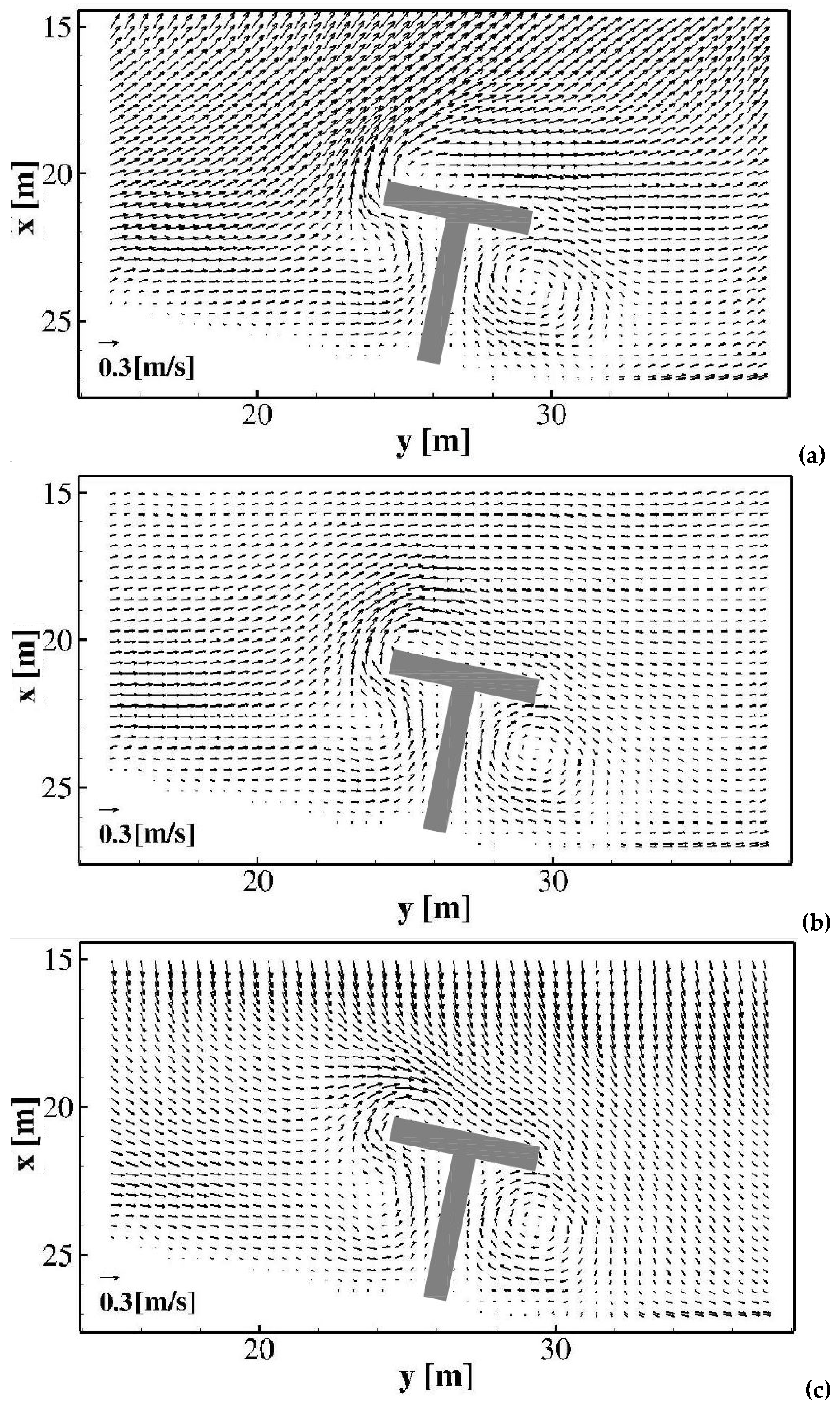
In Figure 2, a plan view of the time-averaged velocity fields at three different position along the vertical direction (near the bottom, at an intermediate position along the vertical direction and near the free surface) is shown. The simulated velocity field is characterized by the presence of an eddy close to the structure, between $x=20 m$ and $x=25 m$ and between $y=27 m$ and $y=32 m$.

From Figure 2a–c, it can be noted that near the bottom the currents are more offshore-directed, while near the free surface the currents are more onshore-directed. From Figure 2b, it can be noted that, at an intermediate position along the vertical direction, the currents are parallel to the shoreline. The different directions of the currents demonstrate the presence of the undertow current, which is offshore-directed near the bottom and onshore-directed near the free surface.

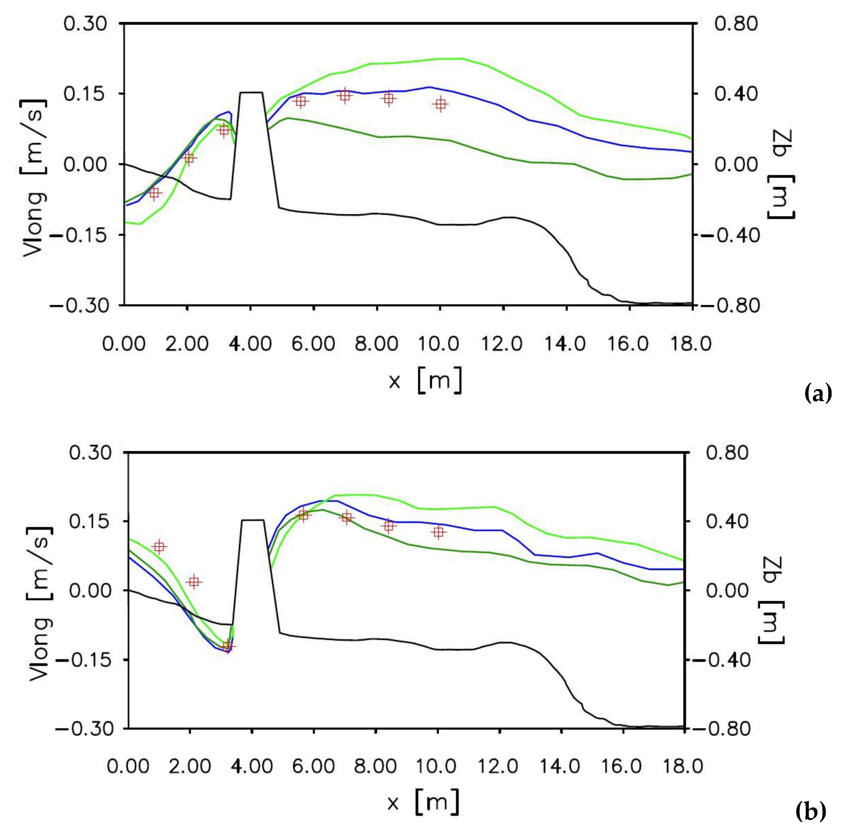
In Figure 3, the comparison between the experimental measurements obtained by [22] and the numerical results in terms of long-shore currents are shown in two different sections $y=22 m$ and $y=26 m$. The blue lines, in Figure 3a,b, show the depth-averaged longshore velocity compared with the experimental measurement (red square). The green lines show the velocity measured at two different position from the free surface, near the bottom $z/z_b=0.894$ (light green line) and near the free surface $z/z_b=0.081$ (green line).

It is possible to notice that the numerical results of the depth-averaged longshore velocity, shown in Figure 3a, slightly overestimate the experimental measurements. From Figure 3b it is possible to notice that the numerical results slightly underestimate the experimental measurements between the shoreline and the T-head groin, while overestimate the same measurements in the offshore zone.

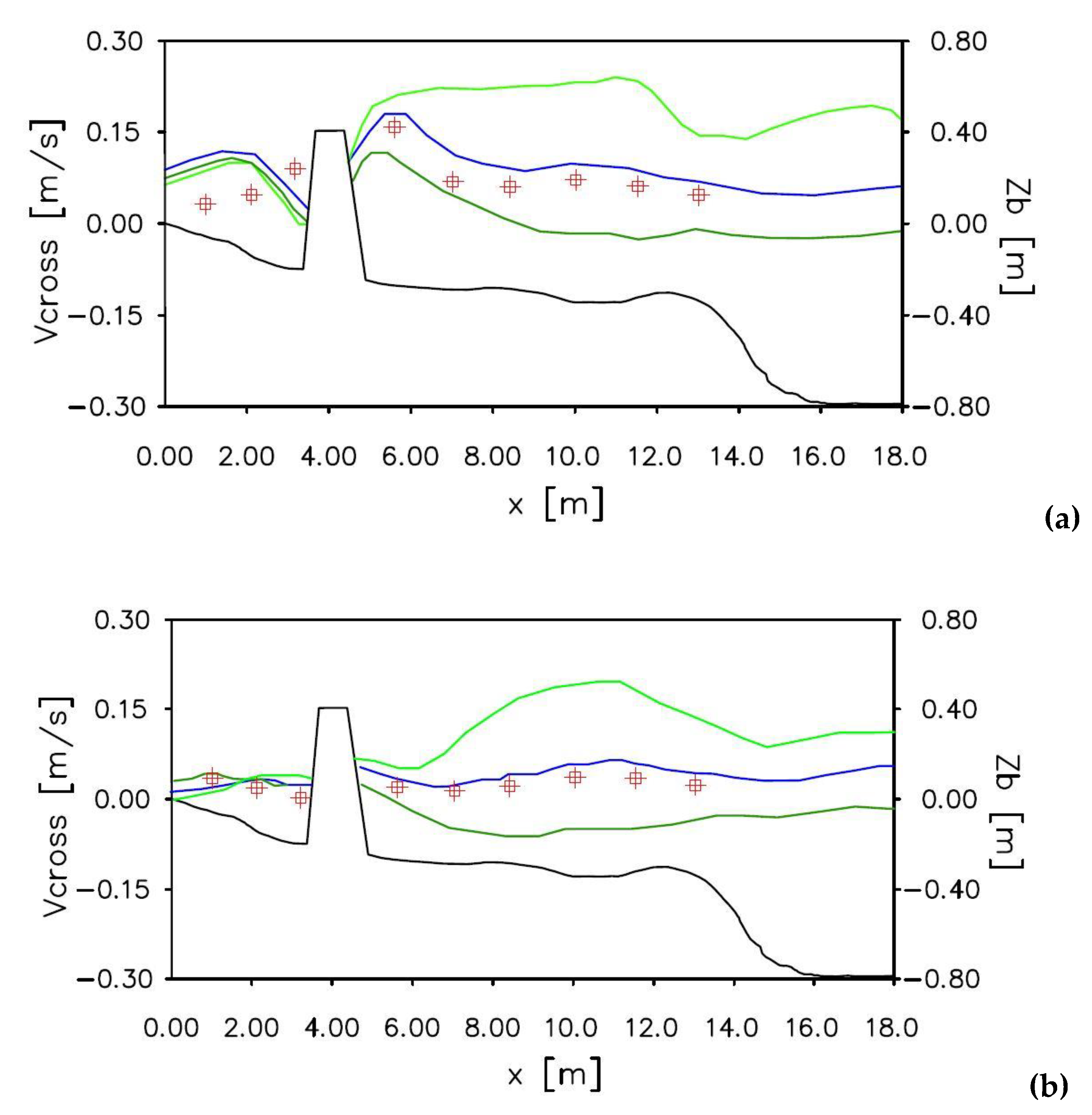
In Figure 4 the comparison between the experimental measurements obtained by [22] and the numerical results in terms of cross-shore currents are shown in two different sections $y=22 m$ and $y=26 m$. The blue lines, in Figure 4a,b, show the depth-averaged cross-shore velocity compared with the experimental measurements (red square). The green lines show the velocity measured at two different position from the free surface, near the bottom $z/z_b=0.894$ (light green line) and near the free surface $z/z_b=0.081$ (green line).

From Figure 4a it is possible to notice that the depth-averaged cross-shore velocity is slightly overestimated by the numerical results from $x=0.0 m$ to $x=3.0 m$, while from $x=5.5 m$ it is slightly overestimated. From Figure 4b it is possible to notice that the depth-averaged velocity is in quite good agreement with the numerical results.

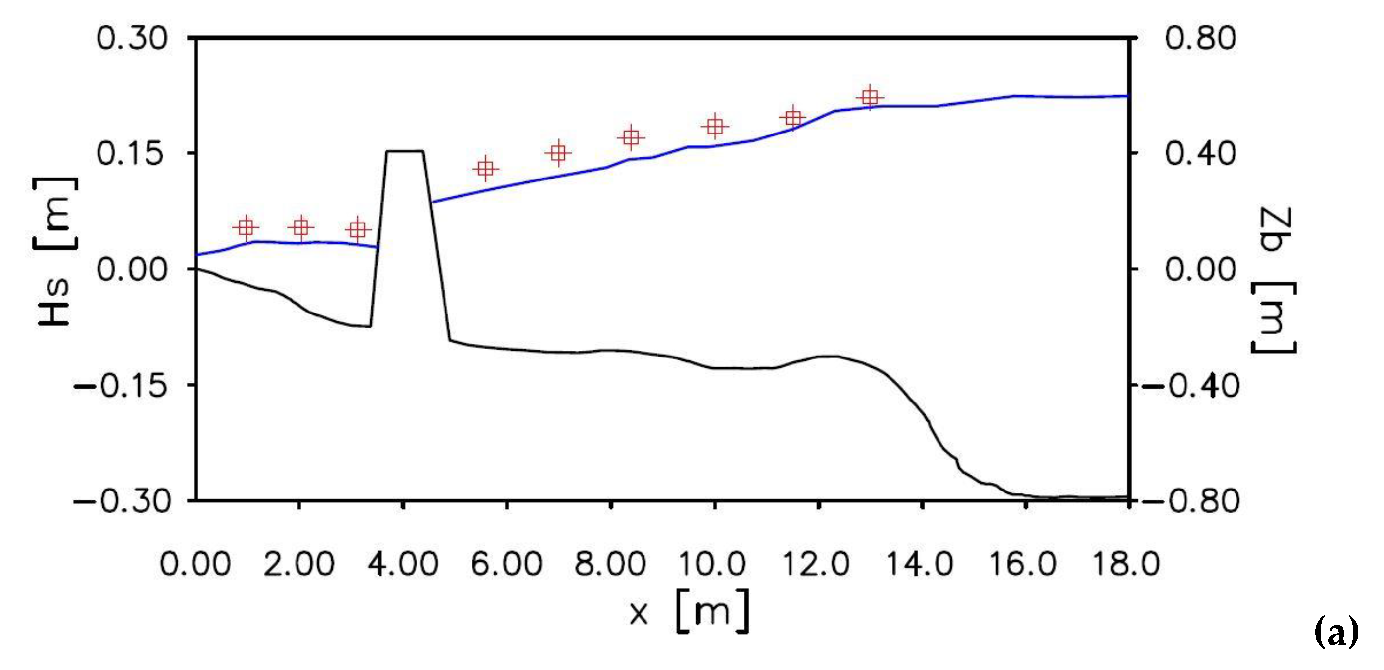
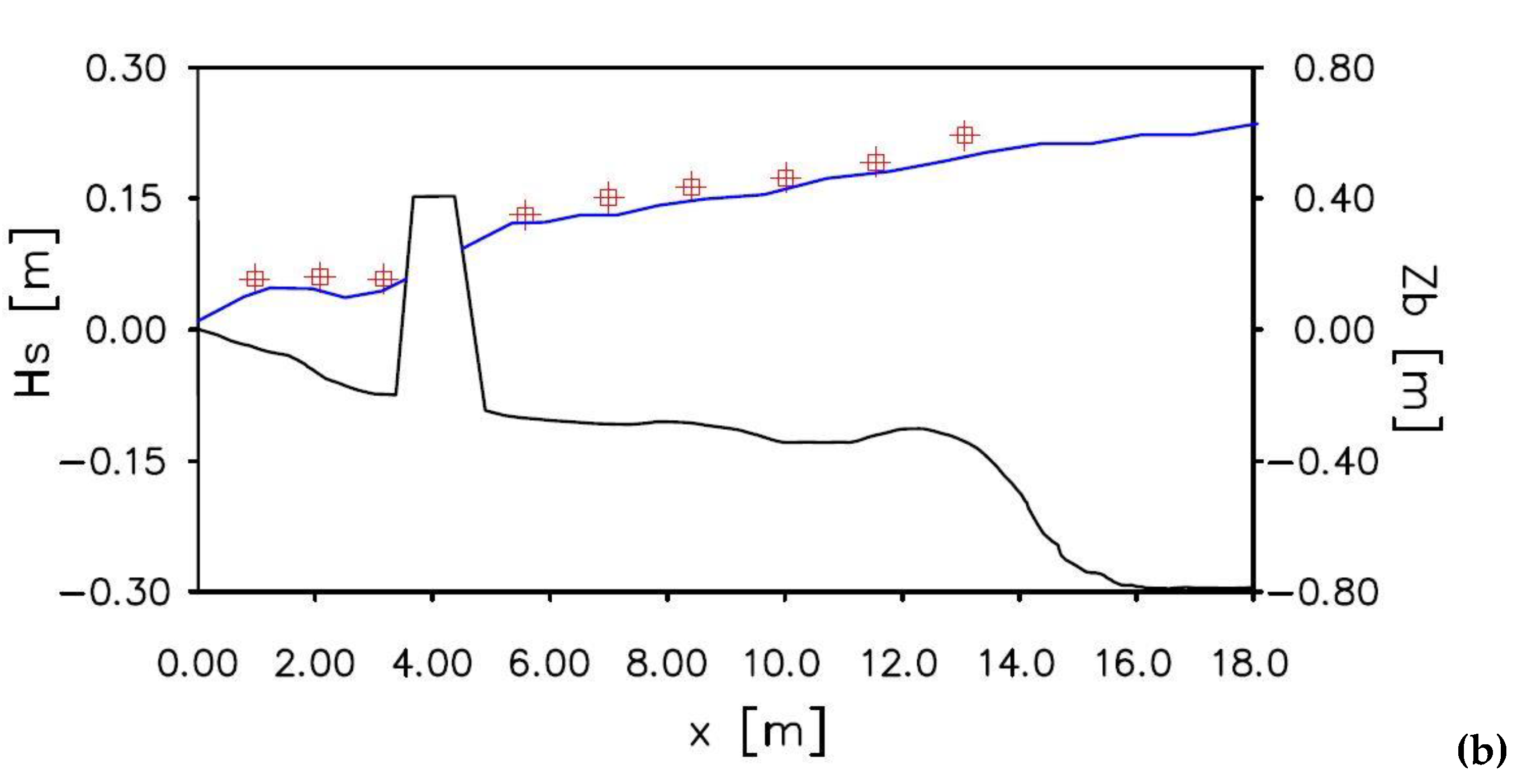
In Figure 5 the comparison between the experimental measurements by [22] and the numerical results in terms of the significant wave height is shown. The results obtained in the sections $y=22m$ and $y=26m$ are shown in Figure 5a,b. Both the comparisons show that the significant wave height obtained by the numerical model is in good agreement with the experimental measurements.

4.3. Wave Induced Currents in the Cetraro Harbour (Italy)

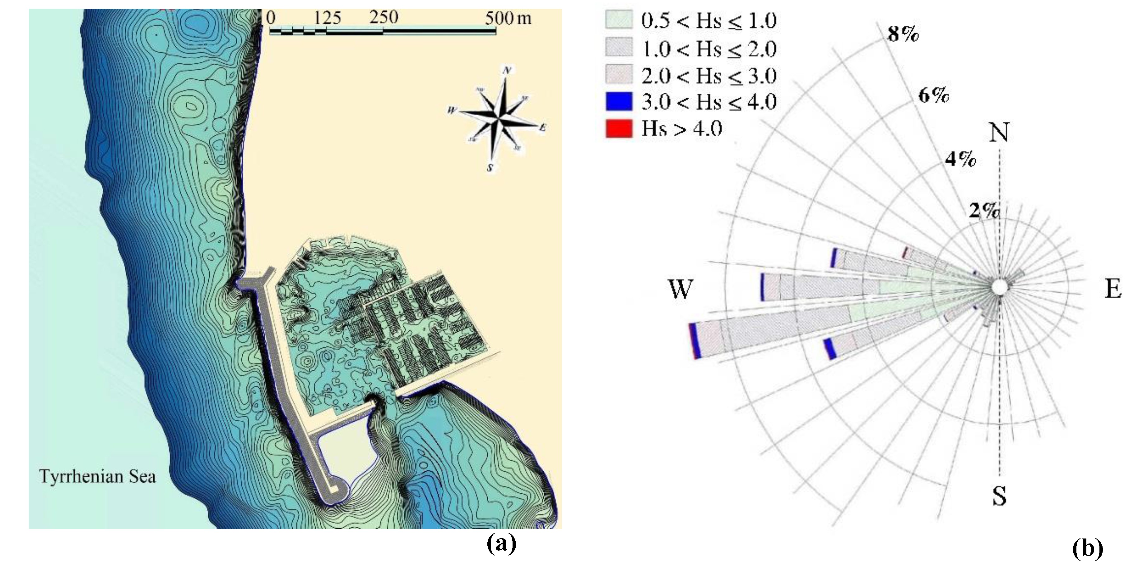
In the present paper the proposed model is used to simulate the wave propagation and wave induced currents in the coastal region of the Cetraro harbour. A plan view of this coastal region is shown in Figure 6a. The numerical simulations are carried out in two different geometric configurations: a first one, denominated present configuration, that reproduces the geometry of the coastal defence structures currently present in the harbour area; a second one, denominated project configuration, that reproduces the presence of a breakwater designed to modify the coastal currents in the area opposite the harbour entrance during the storm events that are considered more significant for the coastal sediment transport.

4.3.1. Wave Fields and Wave Induced Currents in the Present Configuration

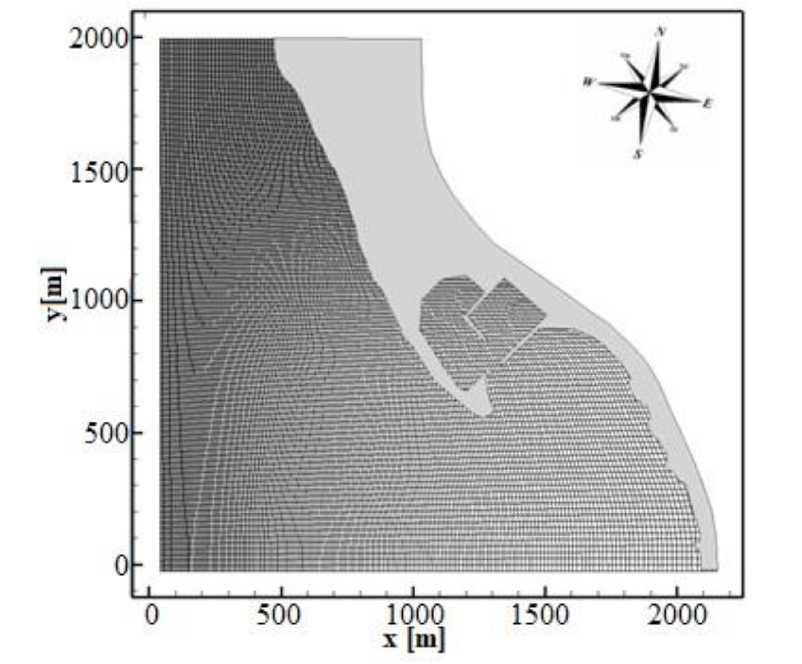
As shown in Figure 6b, in this coastal region, the most frequent waves come from $260°$ North. Among them, the most significant wave event for the coastal sediment transport has a deep-water wave height between 3 m and 4 m. In order to simulate the wave fields and currents, that affect the region of Cetraro harbour during these significant wave event, the physical domain shown in Figure 7 is discretized by a boundary conforming curvilinear grid that reproduces approximatively $2000 m\times 2000 m$ in the horizontal directions. In the present three-dimensional study, the number of grid cells in the horizontal directions are $1152\times 600$.

A plan view of the computational grid that reproduces the present configuration is shown in Figure 7, in which only one curvilinear coordinate line out of 6 is drawn. The spatial step of the grid in the horizontal direction ranges approximatively from $0.9 m$ to $3.2 m$. For the discretization along the vertical direction, just $7$ uniformly distributed grid cells are used. This implies a maximum spatial step in the vertical direction that, in the initial still water condition, ranges approximatively from $1.6 m$ (in the deep-water region) to $0.0125 m$ (near the beach). The left (West) boundary of the computational grid is directed perpendicular to the direction of the significant incoming waves ($260°$ North). Thus, in all the numerical simulations the wave input is assigned on the West boundary, where random waves characterized by a JONSWAP spectrum with peak period equal to $10 s$ and significant wave height equal to $3 m$ are numerically generated. In the North and South open boundaries, zero gradient boundary condition for the free surface and velocity are imposed. The simulated duration of the wave event produced by the above-mentioned input wave is 1 h. By using a $24$ nodes cluster, every simulation lasts approximately $12$ days.

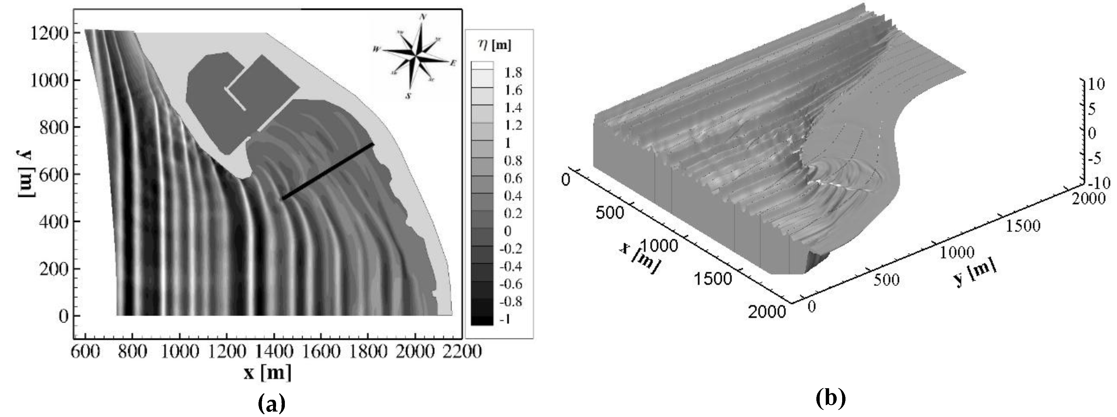
In Figure 8a,b, respectively, a plan view and a three-dimensional view of the wave field obtained by the proposed numerical model in the coastal area of Cetraro harbour during the above-mentioned wave event are shown. From these figures it is possible to see the propagation of the wave fields from the deep water region to the coastline: it can be noted the wave reflection in correspondence of the vertical walls ($700 m<y<900 m$) of the existing breakwater and the wave diffraction around the southern end of it.

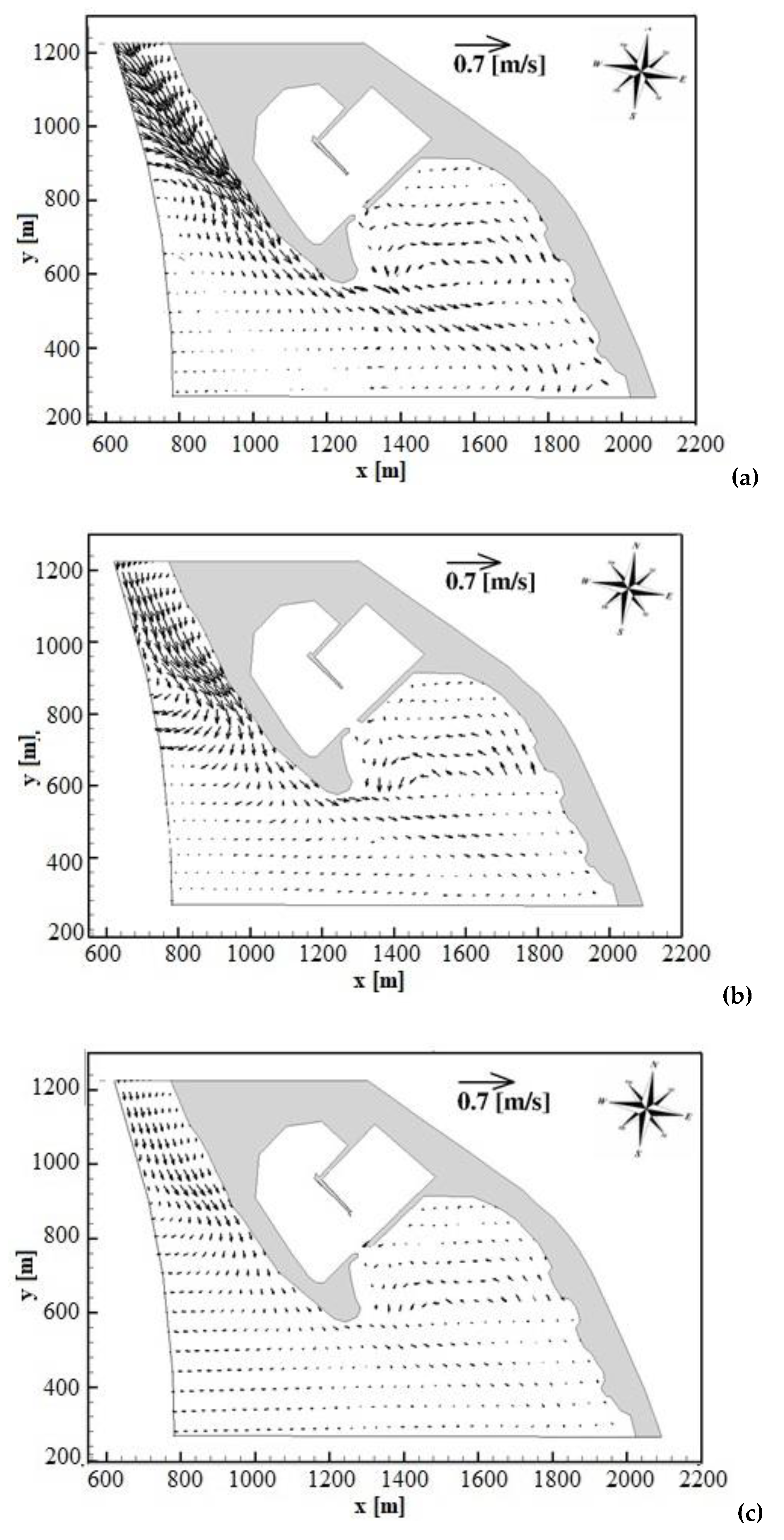
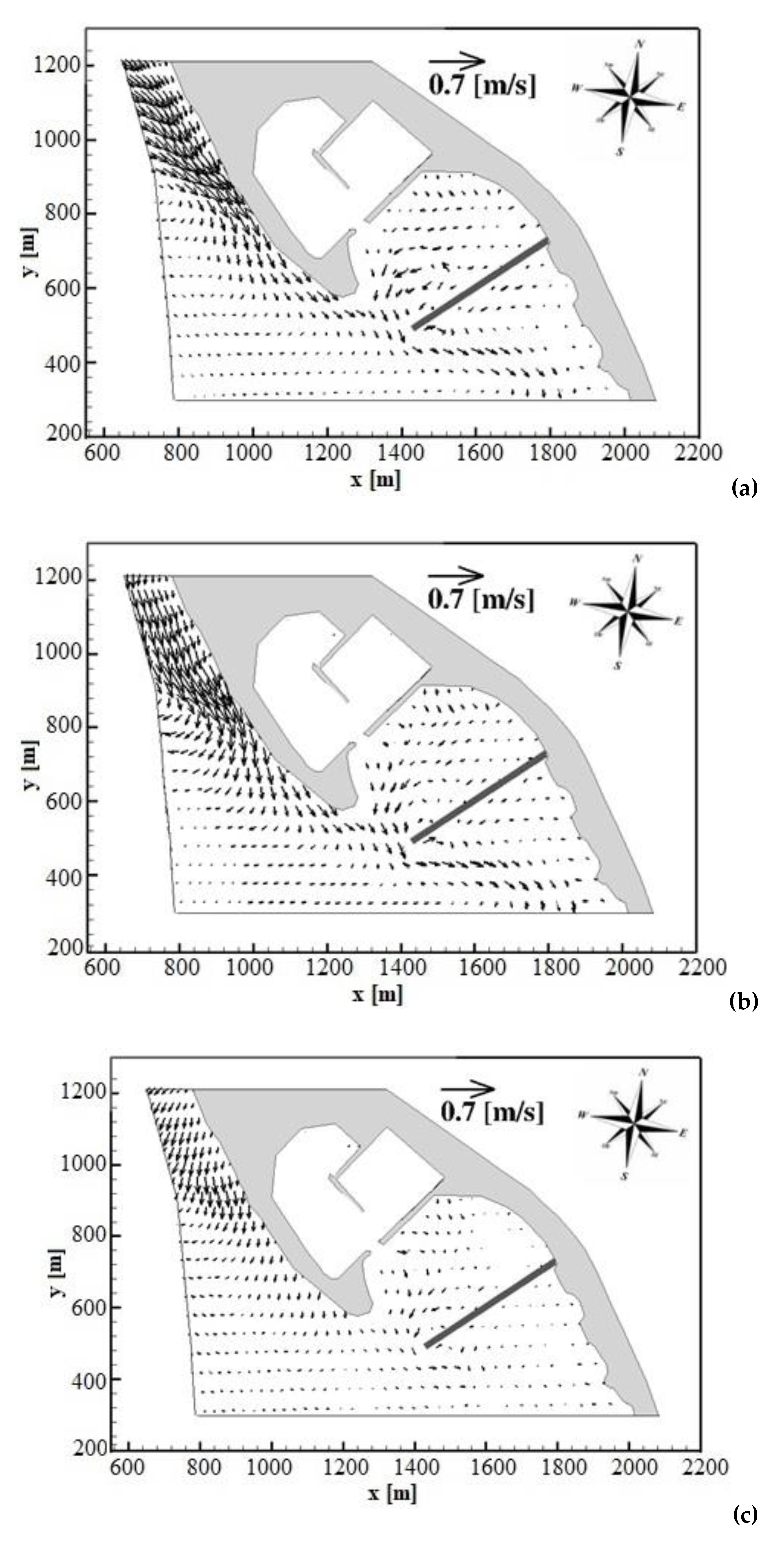
In order to calculate the coastal currents that are produced during the above-mentioned wave event in the Cetraro harbour costal region, for each simulation, after eliminated a simulated transitory period of 30 min, the instantaneous three-dimensional velocity field, obtained during the simulation, are averaged over a further simulated period of 30 min. The results are shown in Figure 9a, where the time averaged velocity fields near the free surface are drawn by black arrows (one velocity out of $15$ is shown). As it is possible to see from Figure 9a, the intensity of this current decreases in the area south of the breakwater, where less steep bottom variations induce less shoaling and breaking phenomena. At the southern limit of the simulated coastal region, where the waves approach to the coastline with a minor incident angle, a smaller intense longshore current can be seen. Furthermore, from Figure 9a it is possible to note that in the coastal area sheltered by the existing breakwater ($x>1300 m$ and $y>600 m$) a significant anticlockwise recirculation pattern of the coastal current occurs. In this area, a current directed from SE to NW along the coastline reaches the area opposite the Cetraro harbour entrance, where it undergoes an anticlockwise rotation.

In this figure it is possible to see that in the northern part of the simulated coastal region a significant longshore current directed from NW to SE takes place during this wave event. In this coastal area the waves approach to the shallow water near the beach with a high incidence angle and undergo a shoaling and breaking phenomenon that is highly not uniform along the y direction. This produces a significant component of the free surface gradient in the longshore direction that drives an intense current in the same direction.

In Figure 9b the time averaged velocity field at intermediate water depth calculated during the numerical simulation is shown. In most of the simulated coastal region, this velocity field is similar to the one calculated near the free surface. The main differences with respect to the latter can be observed in the deep-water region ($x<1400 m$) where the current at intermediate water depth shows a more intense offshore directed component.

In Figure 9c the time averaged velocity field calculated near the bottom is shown. From this figure it can be observed that the structure of the coastal current near the bottom is similar in direction and lower in magnitude with respect to the one calculated at intermediate water. From the numerical results shown in the previous figures it can be deduced that, during the simulated wave event, in the coastal area sheltered by the existing breakwater ($x>1300 m$ and $y>600 m$), in correspondence of the Cetraro harbour entrance, a significant anticlockwise recirculation pattern of the coastal current occurs. Part of this recirculation pattern is due to a current that is directed along the coastline, from SE to NW, and reaches the area opposite the Cetraro harbour entrance, where it undergoes an anticlockwise rotation. In this area, where the wave energy is lower than the one previously described, the sediment picked up by the wave energy in the surf zone and transported by the currents along the coastline tends to settle. The main negative effect of this hydrodynamic process is a progressive silting that affects the area opposite the Cetraro harbour entrance.

4.3.2. Wave Fields and Wave Induced Currents in the Project Configuration

In order to modify the structure of the coastal currents, that take place in this coastal area during the significant wave event and avoid the future siltation of the Cetraro harbour entrance, a new breakwater, approximately $450 m$ long, has been designed. In order to assess the effectiveness of this solution, by the proposed three-dimensional model, a numerical simulation of the wave field and wave induced currents in the project configuration is carried out by imposing the same wave input of the previous configuration, for the same simulated period. In Figure 10a,b a plan view and a three-dimensional view of the wave field obtained by the proposed numerical model, during the above-mentioned wave event, in the Cetraro harbour project configuration is shown. In Figure 10a it is possible to see the position of the designed breakwater (drawn in black).

From these figures (Figure 10a,b) it is possible to see that, the wave field propagation is modified by the presence of the designed breakwater only in proximity of its offshore end, where some wave reflection occurs.

In Figure 11, the simulated time averaged velocity fields, respectively, near the free surface, at intermediate water depth and near the bottom are drawn by black arrows (one velocity out of $15$ is shown).

As can be seen from these figures, the presence of the designed breakwater significantly modifies the structure of the currents in the area of the harbour entrance. In the project configuration, the anticlockwise recirculation pattern that takes place in the area sheltered by the existing breakwater ($x>1300 m$ and $y>600 m$) is limited to the area at the SE of the designed breakwater. The presence of the designed breakwater prevents the SE–NW directed longshore current to reach the Cetraro harbour entrance. This barrier would have the positive hydrodynamic effect of preventing the accumulation of new sediment in the area opposite the Cetraro harbour entrance.

5. Conclusions

A three-dimensional numerical study of the wave field and wave induced currents in a southern Italy coastal area has been proposed. The numerical model is based on an integral and contravariant form of the Navier–Stokes equations in a time dependent curvilinear coordinates system, in which the vertical coordinate moves in order to follow the free surface variations. In the present three-dimensional numerical study, the coastal area opposite the Cetraro harbour has been discretized by a boundary conforming curvilinear grid in which $7$ grid cells are adopted in the vertical direction. By this model, the wave and current fields, that take place in the Cetraro harbour coastal region during the most significant wave event, has been simulated in two different geometrical configurations: a present configuration and a project configuration. The numerical results demonstrate that, during the most significant wave event, the designed breakwater is able to modify the current circulation pattern and can prevent further siltation in the area of the Cetraro harbour entrance. Future developments of the present study will focus on the implementation of a sediment transport model, to be coupled to the hydrodynamic model presented in this paper.

References

- Cannata, G.; Barsi, L.; Petrelli, C.; Gallerano, F. Numerical investigation of wave fields and currents in a coastal engineering case study. WSEAS Trans. Fluid Mech. 2018, 13, 87–94. [Google Scholar]
- Erduran, K.S.; Ilic, S.; Kutija, V. Hybrid finite-volume finite-difference scheme for the solution of Boussinesq equations. Int. J. Numer. Methods Fluids 2005, 49, 1213–1232. [Google Scholar] [CrossRef]
- Chen, Q.; Kirby, J.T.; Dalrymple, R.A.; Shi, F.; Thornton, E.B. Boussinesq modeling of longshore currents. J. Geophys. Res. 2003, 108. [Google Scholar] [CrossRef]
- Cannata, G.; Petrelli, C.; Barsi, L.; Fratello, F.; Gallerano, F. A dam-break flood simulation model in curvilinear coordinates. WSEAS Trans. Fluid Mech. 2018, 13, 60–70. [Google Scholar]
- Zhu, Z.; Yang, Z.; Bai, F.; An, R. A new well-balanced reconstruction technique for the numerical simulation of shallow water flows with wet/dry fronts and complex topography. Water 2018, 10, 1661. [Google Scholar] [CrossRef] [Green Version]
- Fan, C.; An, R.; Li, J.; Li, K.; Deng, Y.; Li, Y. An approach based on the protected object for dam-break flood risk management exemplified at the Zipingpu reservoir. Int. J. Environ. Res. Public Health 2019, 16, 3786. [Google Scholar] [CrossRef] [Green Version]
- Roeber, W.; Cheung, K.F. Boussinesq-type model for energetic breaking waves in fringing reef environment. Coast. Eng. 2012, 70, 1–20. [Google Scholar] [CrossRef]
- Tonelli, M.; Petti, M. Shock-capturing Boussinesq model for irregular wave propagation. Coast. Eng. 2012, 61, 8–19. [Google Scholar] [CrossRef]
- Tonelli, M.; Petti, M. Simulation of wave breaking over complex bathymetries by a Boussinesq model. J. Hydraul. Res. 2011, 49, 473–486. [Google Scholar] [CrossRef]
- Bradford, S.F. Non-hydrostatic model for surf zone simulation. J. Waterw. Port Coast. Ocean Eng. 2011, 137, 163–174. [Google Scholar] [CrossRef]
- Ma, G.; Shi, F.; Kirby, J.T. Shock-capturing non-hydrostatic model for fully dispersive surface wave processes. Ocean Model. 2012, 43–44, 22–35. [Google Scholar] [CrossRef]
- Bradford, S.F. Improving the efficiency and accuracy of a nonhydrostatic surf zone model. Coast. Eng. 2012, 65, 1–10. [Google Scholar] [CrossRef]
- Derakhti, M.; Kirby, J.T.; Shi, F.; Ma, G. NHWAVE: Consistent boundary conditions and turbulence modeling. Ocean Model. 2016, 106, 121–130. [Google Scholar] [CrossRef]
- Cannata, G.; Petrelli, C.; Barsi, L.; Gallerano, F. Numerical integration of the contravariant integral form of the Navier–Stokes equations in time-dependent curvilinear coordinate systems for three-dimensional free surface flows. Contin. Mech. Thermodyn. 2019, 31, 491–519. [Google Scholar] [CrossRef] [Green Version]
- Chen, X.J. A fully hydrodynamic model for three dimensional, free surface flows. Int. J. Numer. Methods Fluids 2003, 42, 929–952. [Google Scholar] [CrossRef]
- Lin, P.; Li, C.W. A σ-coordinate three-dimensional numerical model for surface wave propagation. Int. J. Numer. Methods Fluids 2002, 38, 1045–1068. [Google Scholar] [CrossRef]
- Young, C.C.; Wu, C.H. A σ-coordinate non-hydrostatic model with embedded Boussinesq-type-like equations for modeling deep-water waves. Int. J. Numer. Methods Fluids 2010, 63, 1448–1470. [Google Scholar] [CrossRef]
- Cannata, G.; Gallerano, F.; Palleschi, F.; Petrelli, C.; Barsi, L. Three-dimensional numerical simulation of the velocity fields induced by submerged breakwaters. Int. J. Mech. 2019, 13, 1–14. [Google Scholar]
- Luo, H.; Bewley, T. On the contravariant form of the Navier–Stokes equations in time-dependent curvilinear coordinate systems. J. Comput. Phys. 2004, 19, 355–375. [Google Scholar] [CrossRef]
- Aris, R. Vectors, Tensors, and the Basic Equations of Fluid Mechanics; Dover: New York, NY, USA, 1989. [Google Scholar]
- Ting, F.C.K.; Kirby, J.T. Observation undertow and turbulence in a wave period. Coast. Eng. 1994, 24, 51–80. [Google Scholar] [CrossRef]
- Gravens, M.B.; Wang, P. Data Report: LSTF Experiments—Transport by Waves and Currents & Tombolo Development Behind Headland Structures, Technical Report ERDC/CHLTR-04-9; Coastal and Hydraulics Laboratory, US Army Engineer Research and Development Center: Vicksburg, MS, USA, 2007. [Google Scholar]
Figure 1.
Ting and Kirby [21] breaking wave test case. Phase-averaged wave crest elevations. Experimental data (circles) and numerical results obtained by average fixed value of 40 (solid line).
Figure 2.
Plan view of the time-averaged velocity field: (a) , near the bottom; (b) , intermediate position along the vertical direction; (c) , near the free surface.b.
Figure 3.
Long-shore currents: (a) at , (b) at . Comparison between experimental data by Gravens and Wang [22] (red square) and numerical results of the depth-averaged cross-shore currents (blue line). Numerical results of cross-shore currents near the bottom at a relative distance from the free surface (light green line) and cross-shore currents, near the free surface at a relative distance from the free surface (green line). Bottom profile in black.
Figure 4.
Cross-shore currents: (a) at , (b) at . Comparison between experimental data by Gravens and Wang [22] (red square) and numerical results of the depth-averaged longshore currents (blue line). Numerical results of longshore currents near the bottom at a relative distance from the free surface (light green line) and long-shore currents, near the free surface at a relative distance from the free surface (green line). Bottom profile in black.
Figure 5.
Significant wave height: (a) section at , (b) section at . Comparison between experimental data by Gravens and Wang [22] (red square) and numerical results (blue line). Bottom profile in black.
Figure 6.
(a): Plan view of Cetraro harbour (Italy). (b): Wave height directional distribution offshore Cetraro harbour.
Figure 7.
Plan view of the boundary conforming curvilinear grid adopted for the numerical simulation in the present configuration. One curvilinear coordinate line out of 6 is shown.
Figure 8.
(a) Plan view and (b) three-dimensional view of an instantaneous wave field obtained by the numerical simulation of the significant wave event in the coastal region of Cetraro harbour in the present configuration. : free surface elevation.
Figure 9.
Time-averaged velocity field: (a) near the free surface, (b) at intermediate water depth, (c) near the bottom, obtained by the numerical simulation of the significant wave event in the present configuration of the Cetraro harbour.
Figure 10.
(a) Plan view and (b) three-dimensional view of an instantaneous wave field obtained by the numerical simulation of the significant wave event in the coastal region of Cetraro harbour in the project configuration.
Figure 11.
Time-averaged velocity field: (a) near the free surface, (b) at intermediate water depth, (c) near the bottom, obtained by the numerical simulation of the significant wave event in the project configuration of the Cetraro harbour.
© 2020 by the authors. Licensee MDPI, Basel, Switzerland. This article is an open access article distributed under the terms and conditions of the Creative Commons Attribution (CC BY) license (http://creativecommons.org/licenses/by/4.0/).
Share and Cite
MDPI and ACS Style
Cannata, G.; Palleschi, F.; Iele, B.; Cioffi, F. A Three-Dimensional Numerical Study of Wave Induced Currents in the Cetraro Harbour Coastal Area (Italy). Water 2020, 12, 935. https://doi.org/10.3390/w12040935
AMA Style
Cannata G, Palleschi F, Iele B, Cioffi F. A Three-Dimensional Numerical Study of Wave Induced Currents in the Cetraro Harbour Coastal Area (Italy). Water. 2020; 12(4):935. https://doi.org/10.3390/w12040935
Chicago/Turabian StyleCannata, Giovanni, Federica Palleschi, Benedetta Iele, and Francesco Cioffi. 2020. "A Three-Dimensional Numerical Study of Wave Induced Currents in the Cetraro Harbour Coastal Area (Italy)" Water 12, no. 4: 935. https://doi.org/10.3390/w12040935
Note that from the first issue of 2016, this journal uses article numbers instead of page numbers. See further details here.