Application of Empirical Mode Decomposition Method to Synthesize Flow Data: A Case Study of Hushan Reservoir in Taiwan


Department of Harbor and River Engineering, National Taiwan Ocean University, Keelung 20224, Taiwan
*
Author to whom correspondence should be addressed.
Water 2020, 12(4), 927; https://doi.org/10.3390/w12040927
Submission received: 7 March 2020
/
Revised: 19 March 2020
/
Accepted: 19 March 2020
/
Published: 25 March 2020
(This article belongs to the Special Issue Advances in Hydrologic Forecasts and Water Resources Management )
Abstract
:Although empirical mode decomposition (EMD) was developed to analyze nonlinear and non-stationary data in the beginning, the purpose of this study is to propose a new method—based on EMD—to synthesize and generate data which be interfered with the non-stationary problems. While using EMD to decompose flow record, the intrinsic mode functions and residue of a given record can be re-arranged and re-combined to generate synthetic time series with the same period. Next, the new synthetic and historical flow data will be used to simulate the water supply system of Hushan reservoir, and explore the difference between the newly synthetic and historical flow data for each goal in the water supply system of Hushan reservoir. Compared the historical flow with the synthetic data generated by EMD, the synthetic data is similar to the historical flow distribution overall. The flow during dry season changes in significantly (±0.78 m3/s); however, the flow distribution during wet season varies significantly (±0.63 m3/s). There are two analytic scenarios for demand. For Scenario I, without supporting industrial demand, the simulation results of the generation data of Method I and II show that both are more severe than the current condition, the shortage index of each method is between 0.67–1.96 but are acceptable. For Scenario II, no matter in which way the synthesis flow is simulated, supporting industrial demand will seriously affect the equity of domestic demand, the shortage index of each method is between 1.203 and 2.12.
1. Introduction
Water resources are necessary for human survival, and are an important part of maintaining socio-economic development and the sustainability of the ecological environment as well. Taiwan is located at the border of tropical and subtropical areas. The main source of water resources is rainfall. The annual average rainfall in Taiwan is about 2500 mm, which is 2.5 times of the world’s average. In recent years, statistics show that rainfall characteristics have become more extreme in Taiwan. Not only the raining days gradually decreasing, but the intensity gradually is increasing. On the whole, although Taiwan seems to be a country with abundant rainfall, the overall water resources environment is not easy to manageme because of climate change.
The impact of climate change tends to cause non-stationary conditions in hydrological data. Traditionally, hydrological analysis and data generation only deal with stationary data. Empirical mode decomposition (EMD) can be applied to any type of signal decomposition. Unlike singular spectrum analysis, Fourier transform, and Wavelet transform, EMD does not require any pre-determined basis functions and can extract intrinsic mode function (IMF) components from the original signal in a self-adaptive way [1]. Through the characteristics of EMD, non-stationary and nonlinear signals can be processed, which effectively overcomes the limitations of traditional methods.
EMD has been proposed [2] as an adaptive time-frequency data analysis method. In this study, the EMD method and the decomposed IMFs were used for data analysis and synthesis. Many studies use EMD to analyze different time series and decompose the implied fluctuation periods [3,4,5,6]. In recent years, there are many carefully studies of nonlinear and non-stationary for the hydrological field: Lee and Ouarda [7,8] proposed model reproduces Nonstationary oscillation (NSO) processes by utilizing EMD and nonparametric simulation techniques; Molla et al. [9,10] show that the EMD successively extracts the IMFs with the highest local frequencies in a recursive way, which yields effectively a set low-pass filters based entirely on the properties exhibited by the data. In addition, there are many studies based on the EMD method to predict and estimate streamflow data: Huang et al. [11] and Meng et al. [12] developed a modified EMD-based support vector machine for non-stationary streamflow prediction; Zhang et al. [13] improved the efficiency of a prediction approach which can be used as a general technique for non-stationary time series forecasting.
However, the mode mixing problem may occur during the EMD. To avoid mode mixing, Wu and Huang [14] proposed a new noise-assisted data analysis method, the Ensemble EMD (EEMD), which defines the true IMF components as the mean of an ensemble of trials, each consisting of the signal plus a white noise of finite amplitude. Zhao and Chen [15] and Zhang et al. [16] used the EEMD and other methods to build a hybrid model for annual runoff time series forecasting. Many of EEMD applications in hydrology focus on the diagnostic analysis of historical data, such as features of temperature variation trends [17], forward prediction of runoff data in data-scarce basins [18], and forecast monthly reservoir inflow [19].
The analysis methods of water resources allocation system are mainly divided into two categories: simulation method and optimization method. Yeh [20] and Wurbs [21] introduced the theory development of the simulation model and optimization model in reservoir system analysis. Chang et al. [22] present the usefulness of the neural network in deriving general operating policies for a multi-reservoir system. An optimization-based approach is typically required for the optimal operation of a reservoir system, in order to obtain the optimal solutions to support the decision-making process [23]. In this study, we use the simulation method for the analysis of water resources systems. Lee and Huang [24] evaluated the impact of climate change on the water supply of the reservoir in central Taiwan.
The Hushan reservoir is a new water supply resource system in central Taiwan (Figure 1). Since some problems exist in the water supply system of the Zhuoshui river, such as its high concentration of sediment, and low efficiency for the Hushan reservoir while it considers a joint operation with Jiji weir [25]. Therefore, Chu and Huang [26] recommends the Hushan reservoir should operate independently. Under the assumption that simulation results show that the Hushan reservoir is capable of supplying more than 100,000 m3 per day (up to 380,000 m3/day) and the reservoir utilization rate can reach 2.41 from 1.18 while Shortage Index (SI) = 1.
This study proposes a novel procedure, which is based on EEMD and its derivation (IMF and residue) as an implement for synthesizing non-stationary data, which will be applied in reservoir inflow and impact assessment for water supply. This study will continue the research results of Huang et al. [27]. Huang et al. [27] proposed a surface temperature and rainfall synthesis method base on EMD. The method utilizes the recombination of the IMF of the segmented data, as well as the characteristics of the residuals to generate the data. There is a plan to use the IMFs and residues obtained, after EMD decomposition to permutation and combination, to generate new flow data. There is also a plan to try to apply the newly synthetic flow data to simulate the water supply system of the Hushan reservoir (as shown in Figure 1). Finally, several evaluation indicators are used to evaluate water supply system simulation results.
2. Materials and Method
2.1. Study Area
2.1.1. Hushan Reservoir
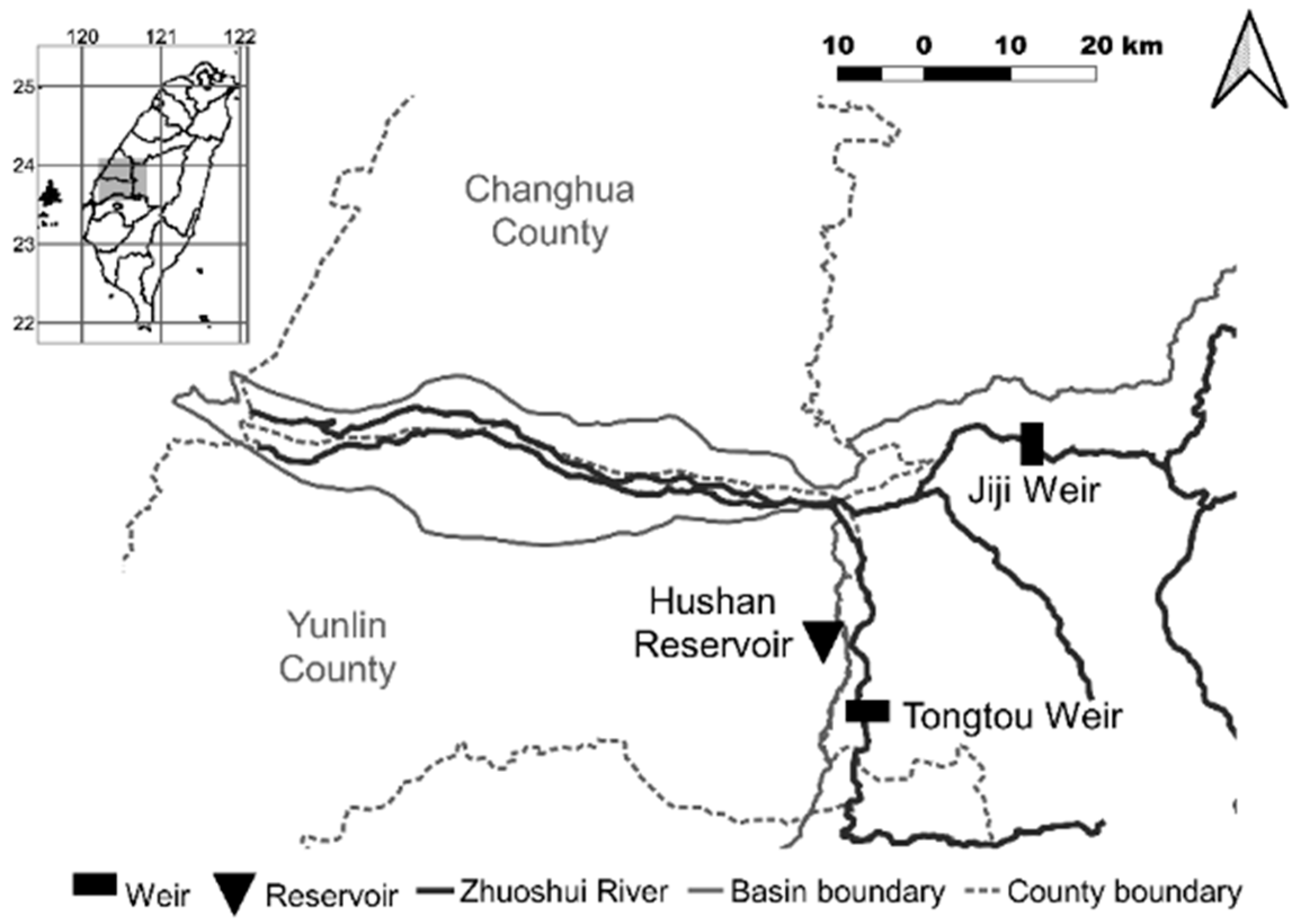
Hushan reservoir is an off-channel reservoir. It is located between Douliu City and Gukeng Township, Yunlin County, 10 km southeast away from the Douliu City center (as shown in Figure 2). The reservoir was set up in 2016 and first reached its full water level in June 2019. The main purpose of the Hushan Reservoir is to reduce pumping groundwater and to slow down the problem of land subsidence in Yunlin county. The elevation-area-capacity relationship of Hushan Reservoir is shown in Table 1. The elevation of the remaining water level is 165 m, the full water level is 211.5 m, and the effective storage capacity of the reservoir is 53.47 × 10⁶ m3. The elevations of the water outlets are 165 m and 180 m respectively. The designed flow of the domestic water channel and the permanent river outlet are 12.27 m3/s and 1.00 m3/s, respectively. The watershed of Hushan reservoir is only 6.58 km2 and leads to limited water resources. Therefore, the Tongtou weir, the intake of Hushan reservoir, on the Qingshui river needs to be guided through the diversion tunnel.
2.1.2. Tongtou Weir
Tongtou weir is the intake of Hushan reservoir. In order to ensure the river base flow and the downstream water requirements—such as agriculture and domestic—of Tongtou weir will be satisfied. The weir diversion operation will give priority to the base flow and water right; next, the intake of Hushan reservoir from Tongtou weir on Qingshui river be considered. The plan of the Tongtou weir diversion water accounts for about 10% of the Qingshui river during the wet season (May to October), and about 13% during the dry season. The Tongtou weir is located 70 m downstream of the Tongtou suspension bridge in the Qingshui river. There is a sedimentation basin before the water be taken from Tongtou weir to Hushan reservoir. The intake channel is 2.8 km long and designed intake capacity is 20 m3/s, with a gravity type.
2.2. Research Method
2.2.1. Empirical Mode Decomposition
EMD is proposed for nonlinear and nonstationary time series analysis [2]. For the hydrological time series, EMD divides the sequence into two parts: IMFs and residue. The IMFs represent the implied period sequence of the data, and the residue represents the non-period sequence of the data. Although the methods used in traditional signal analysis fields such as fast Fourier transform, harmonic analysis, and wavelet analysis can also express the original sequence as a superposition of multiple period functions; these Fourier basic function-based analyses usually only deal with stationary time series. Contrary to the previous methods, EMD is intuitive, direct, a posteriori, and adaptive, with the basis of the decomposition based on, and derived from, the data [2]. EMD is more suitable for analyzing non-stationary hydrological time series.
EMD decomposes the original signal into different time scale of oscillation components called IMF. Unlike singular spectrum analysis, Fourier transform, and Wavelet transform, EMD does not require any pre-determined basis functions and can extract IMF components from the original signal in a self-adaptive way [1]. Each IMF component should satisfy the following two conditions:
- In the whole data series, the number of extrema and the number of zero-crossings must either equal or differ at most by 1;
- At any point, the mean value of the envelope defined by the local maxima and the envelope defined by the local minima is zero.
An IMF represents a simple oscillatory mode as a counterpart to the simple harmonic function, but it is much more general. For time series data x(t) (t = 1, 2, …, n), the procedure of EMD can be described as follows [16]:
- Identify all the local maxima and minima of the original time series ;
- Using the three-spline interpolation function to create the upper envelopes and the lower envelopes of the time series;
- Calculate mean value m(t) of the upper and lower envelopes ;
- Calculate the difference value d(t) between time series x(t) and mean value m(t), ;
- Check the difference value d(t): (a) if d(t) satisfies the two IMF conditions, then d(t) is defined as the ith IMF, the residue replace the x(t). The ith IMF is denoted as ; (b) if d(t) is not an IMF, then d(t) replace the x(t).
- Repeat (1)–(5) until the residue item r(t) becomes a monotone function or the number of extrema is less than or equal to 1, so that the IMF component cannot be decomposed again.
Finally, original time series x(t) can be denoted as sum of IMFs and residue r(t).
where n, and represent the number of IMF, the ith IMF and the residue, respectively. The residue also represents the overall trend or the mean value of the original time series data. Figure 3 shows the results of the EMD method decomposition.
2.2.2. Ensemble Empirical Mode Decomposition
EEMD, an improvement of EMD, was proposed by Wu and Huang [14]. Although EMD has obvious advantages in signal analysis, there are unavoidable defects such as the boundary-effect and mode-mixing. Mode mixing is a problem often encountered when using EMD to decompose sequences. Mode mixing means that a certain IMF contains waves with very different periodicity, often caused by intermittent signal interference. In particular, the mode-mixing will not only cause the mixing of various scale vibration modes but can even lose the physical meaning of individual IMF. To overcome this problem of the EMD method, a new noise-assisted data analysis method is proposed—the EEMD [14]—which defines the true IMF components as the mean of an ensemble of trials, each consisting of the signal plus a white noise of finite amplitude.
The main step of EEMD is described as follows [16]:
- Add white noise w(t) to the original time series x(t). The new time series can be defined as:
- Decompose the new time series into IMFs using EMD method;
- Repeat steps (1) and (2) with different white noises series each time;
- Obtain the mean of the ensemble corresponding IMFs of the decompositions as the final result.
Differently from EMD, the EEMD method first adds white noise to the original data before decomposition and uses the statistics feature of white noise, the expectation is equal to zero, to perform the screening process. After adding white noise many times, the effect of adding white noise will be offset by the mean of the ensemble IMF. Therefore, the decomposition using EEMD not only keeps the inherent feature of the original signal, but also overcomes the mode-mixing.
The effect of the added white noise should decrease using the equation [14]
where N is the number of ensemble members, is the amplitude of the added noise and is the final standard deviation of error, which is defined as the difference between the input signal and the corresponding IMF(s). According to Equation (3), when the average number of times increases, the error will reduce, and when n reaches a certain number of times, its error value can be ignored.
2.2.3. Zero Up-Cross Method
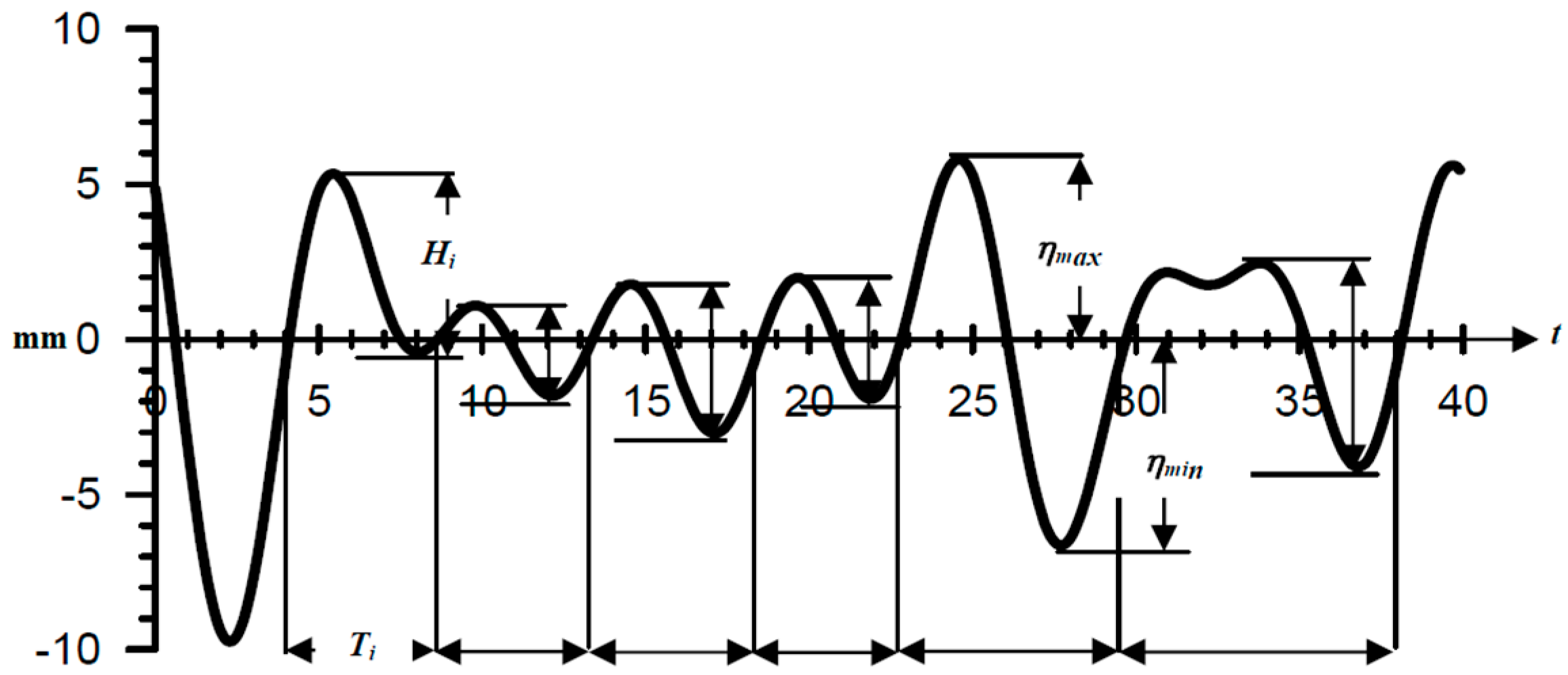
Statistical analysis of a IMF, a wave set, requires establishment of the definition of individual wave heights and periods. The standard is the employment of the zero-crossing definition. The zero line or the line of the mean wave level is set for a record of wave registration, and each wave is defined with the reference point where the instantaneous water level crosses the zero line. When the upward crossing point is employed as the beginning of an individual wave, the method is called the zero up-crossing method [28]. The definition of upward crossing point is [29]
where is the wave height in given time.
The wave period, T, of an individual wave will be defined as the time between two successive upward crossing point, as Figure 4 showing. For any individual wave, the peak and valley are expressed as
The average value of the highest point (peak) and the lowest point (valley) of is used as the amplitude of each wave, as shown in Equation (7)
In this study, we use the IMF decomposed by the EEMD to perform a zero up cross analysis method, analyze the periods of each IMF, and discuss it.
After finding the period in the fluctuation using the zero up cross analysis method, the sum of squares of each IMFs is regarded as its energy, and its value can correspond to the period relationship in the fluctuation. The total energy value of each group is added up to form the IMF percentage of each group compared with the energy of each group. The relational expressions of the energy percentages are
where is the square value at each time point of each group of IMF; is the total energy; is weight of energy.
2.2.4. Data Synthesis
The impact of climate change tends to cause non-stationary conditions in hydrological data. Therefore, we use the EEMD [14] in this study, and proposes a new way to synthesize and generate data that can solve the non-stationary data problems. For a given flow time series, the IMFs and residue, the EEMD decomposed result, would be replace by corresponding component in another period; next, the new combination of IMFs and residue are summed up according to the completeness of EMD [2]; then, the synthetic new flow time series will be produced. Thus, if there are many EEMD decomposed results with the same length but different period, we could synthesize a flow data set through permutation and combination of the corresponding IMFs and residues.
In this study, the historical 60-year (1956–2015) flow data of Tongtou streamflow gauge are segmented in groups of 10 years. Through the EEMD method divides the sequence into two parts: IMFs represent the inherent period sequence of the data, and the residue represents the non-period sequence of the data. We can go through the permutations and combinations of the IMFs to get sequences. Where n is the number of groups of data grouping; i is the number of IMFs by the group.
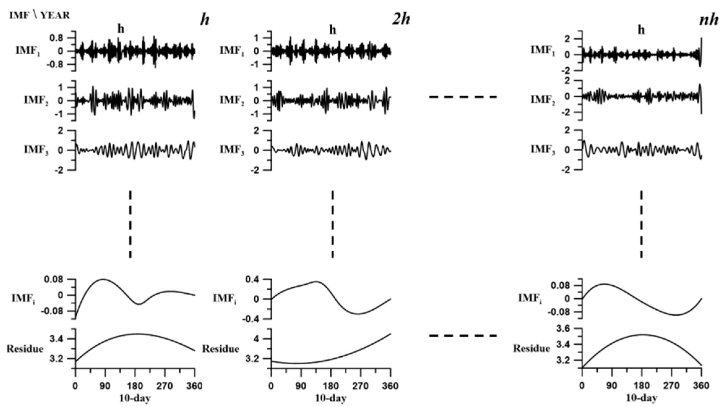
After completing the permutations and combinations of IMFs as shown in Figure 5, we can get the new synthesis data of equal length streamflow. In this study, two permutations and combinations methods are used to synthesize new 10-year flow series data. The method is described as follows:
- Regression analysis is performed on the different residue of each group to fit a new residue to represent the residue value. By adding the results of the IMFs permutation and combination with the representative values of the residue, we can get 10-year new synthetic flow data for the groups.
- Permutation and combination of the different remainders of each group with IMFs, we can get 10-year new synthetic flow data for the groups.
2.2.5. Water Supply System Simulation of Hushan Reservoir
The simulation method is commonly used in the analysis of water resources systems. It conceptualizes the actual operation of the system to explore the use of water resources. In this study, we use the simulation method to simulate the water supply system and explore the difference between the newly synthesized flow data for each goal in the water supply system of Hushan reservoir.
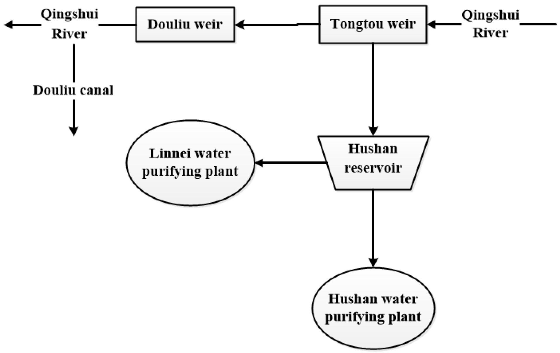
First of all, the historical (1956–2015) flow data of Qingshui river were used to simulate accordance with the Hushan reservoir operation rules. Because the Hushan reservoir takes water from the Qingshui river through a water diversion tunnel, and there is some agricultural water right downstream of the Tongtou weir (as shown in Figure 6). Therefore, before taking water to the Hushan reservoir, Tongtou weir has to consider and satisfy the agricultural water downstream. The remaining flow is the amount of water that can be taken to the Hushan reservoir. The main thing of simulation is that the water taken into the Hushan reservoir should not affect the downstream agricultural water right.
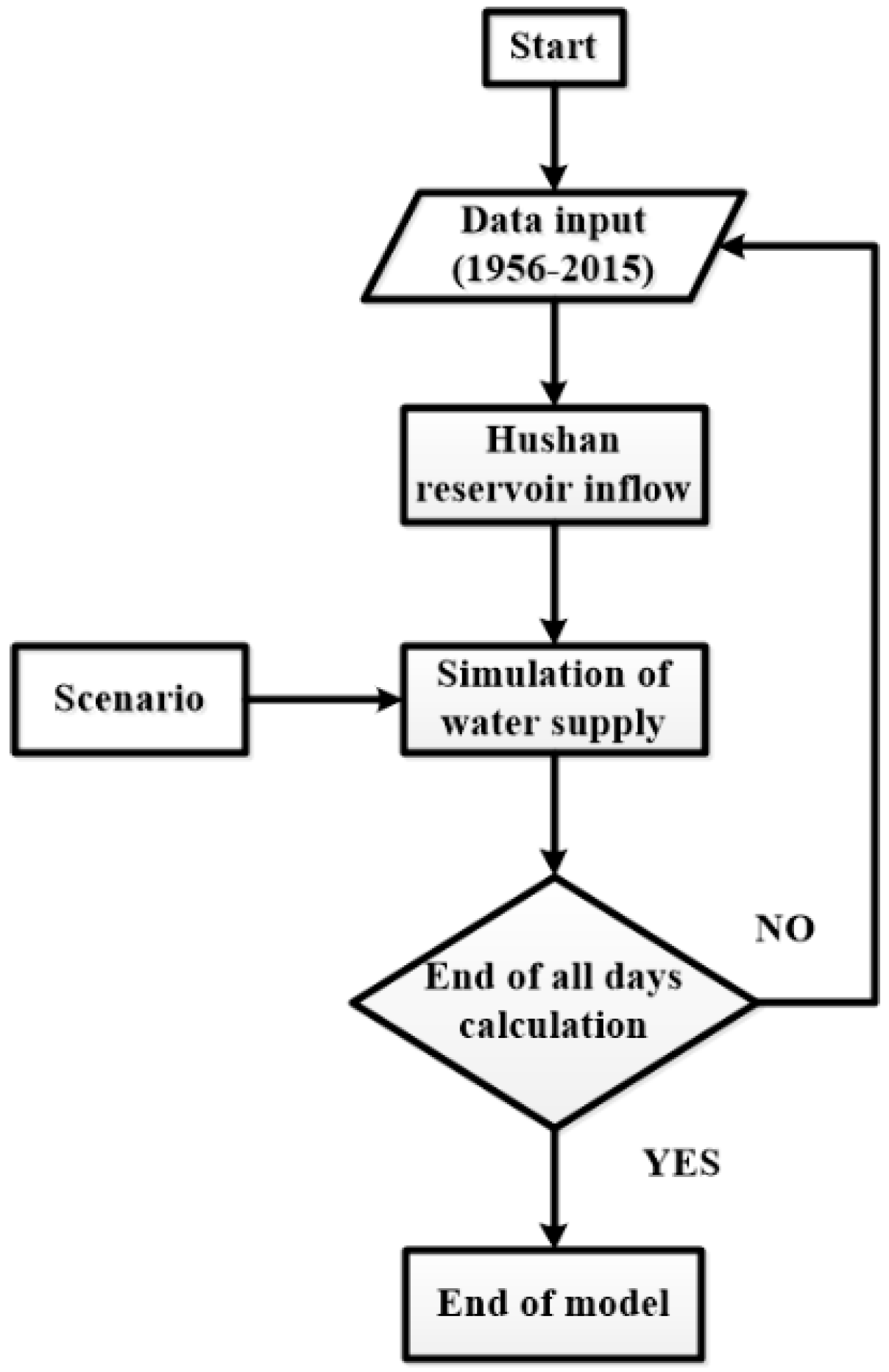
This study will assume different scenarios to simulate the water supply system of Hushan reservoir. The main difference of these two scenarios is the object of water supply (as shown in Table 2). The local water supply system is shown in Figure 6, and the simulation program calculation process is shown in Figure 7.
In the past, the Linnei water purifying plant only supplied 1.2 × 10⁵ m3 water per day, and the deficit of demand was filled by pumping groundwater. After the completion of the Hushan reservoir, the situation of over pumping will be improved. The Hushan reservoir was originally intended to be used in conjunction with the Jiji weir to supply water for domestic demand in the Yunlin area. However, the conjunction operation of Hushan reservoir and Jiji weir will result in a low reservoir utilization rate of only 1.18 [25]. Therefore, we assume the Hushan reservoir operates independently in this study. The domestic demand in the Yunlin area is 2.8 × 10⁵/day, and the support demand for industrial is 3.0 × 10⁵/day. Based on the previous study, the operational regulations of reservoir were added [26], and the upper and lower rule curve is set at the water level of 190 m and 185 m for Hushan reservoir, respectively. In order to explore the situation of water resources utilization in the Yunlin area of the Hushan reservoir under different demand scenarios, the operation of reservoir should follow these principles:
- Supply of the Hushan reservoir must not be less than the projected demand if the water surface elevation exceeds the upper curve.
- Supply of the Hushan reservoir should satisfy 100% of the projected domestic demand, 90% of the projected industrial demand, and 50% of the projected irrigation demand if the water surface elevation is between the upper and lower curve.
- Supply of the Hushan reservoir should satisfy 80% of the planning domestic demand and 0% of the projected irrigation and industrial demand if the water surface elevation is under the lower curve.
2.2.6. Indices for Impact and Risk Assessment
To assess the impact and the risk under different scenarios, the shortage index (SI), satisfaction and reliability of the water supply were determined. Equations (10)–(16) define these indices.
- Satisfaction:
- Reliability:
- Shortage Index:where and are the quantities of water demand and supply, respectively; N is the given time scale of the simulation, and is the number of days for which the demand has been satisfied.
- Reservoir Efficiency:
- The average duration of water shortage events:where M is the number of occurrences of water shortage events, is the duration of each water shortage event, is the average duration of water shortage events.
- The average water shortage in the water shortage event (106 m3):where is the total water shortage in each event, and is the average water shortage in the water shortage event.
- The daily average water shortage in the water shortage event (106 m3/day):
3. Results and Discussion
3.1. 60-Year Flow Data Analysis with EEMD
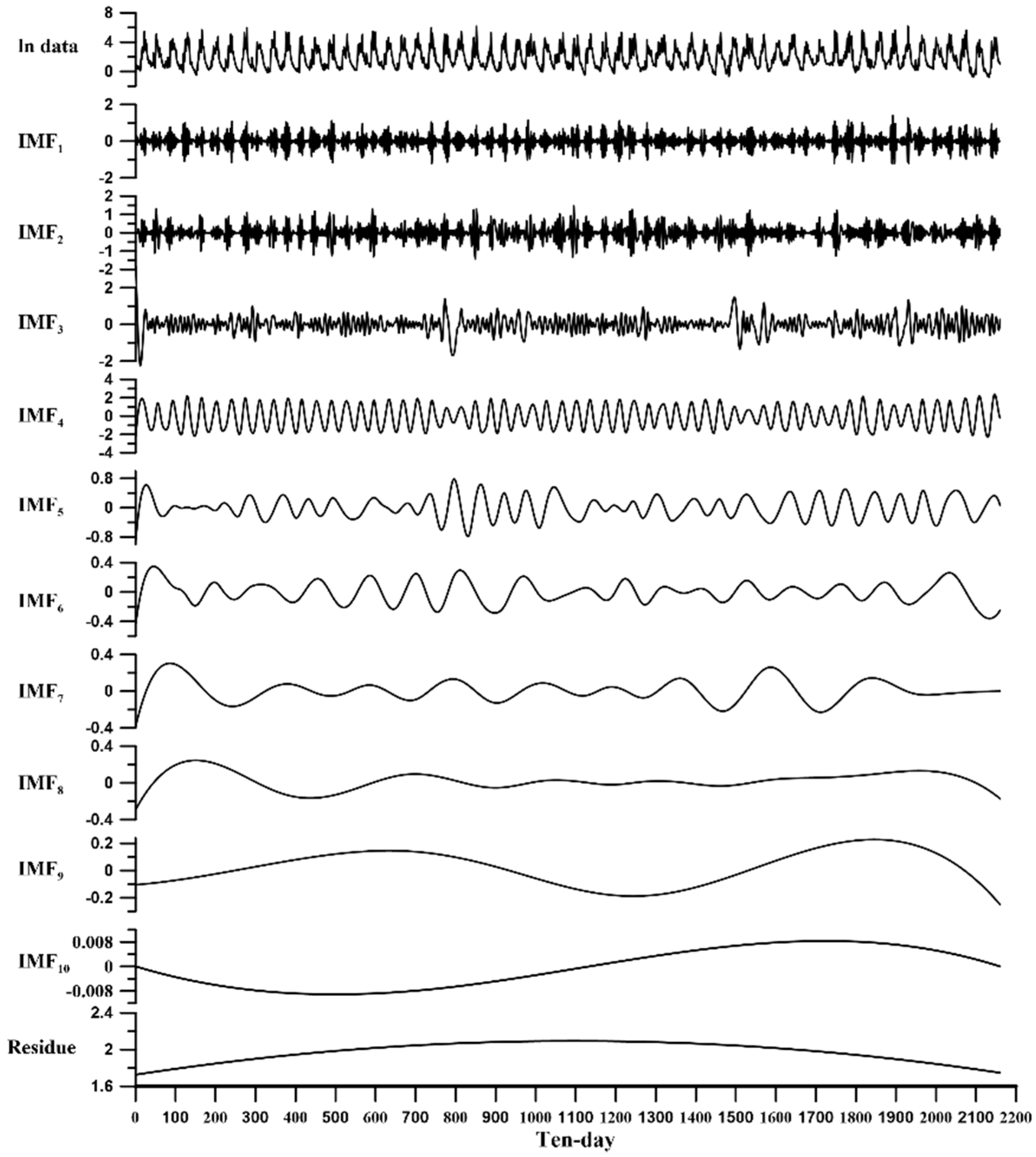
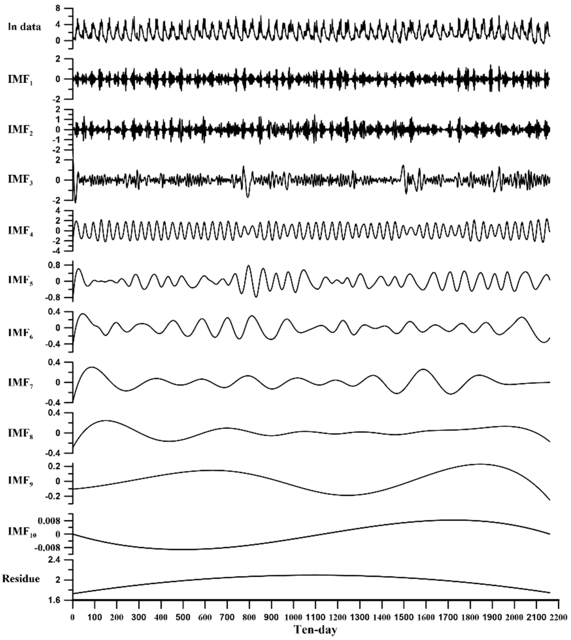
We analyze the historical flow data from 1956 to 2015 in this study. Because the skewness of flow data will affect the decomposition process, the historical flow data is taken nature log transformation before decomposing by the EEMD. The 60-year historical data is decomposed by the EEMD method, and the decomposed IMFs are shown in Figure 8.
Figure 8 shows that there are 10 IMFs and 1 residue. The termination condition of the EEMD is according to following literatures: Wu and Huang [14] show that the number of IMFs approaching can be obtained by EEMD decomposition of the original data; in addition, Huang et al. [27] also explained that the IMF obtained after the data is decomposed will be between and . Therefore, the result that deals with 60-year daily flow by EEMD will introduce 10 IMFs and 1 residue. Among them, the oscillation of IMF1–IMF10 gradually decrease from ± 3 to ± 0.008, but the range of the residue gradually increased from 1.73 to 2.09 and then decreased to 1.75, which is a monotonic function. From the decomposition, we can find that the residue part plays an important role, which often affects the trend of whole time series.
Historical flow data is regarded as a signal for a certain period of time. After decomposing the flow data through EEMD, the physical meaning of IMFs will be diagnosed. The period of each IMF is estimated according to zero up-cross analysis. However, the true energy value cannot be calculated, the square of the IMF value only be regarded as direct proportion with the true energy. In other words, the energy representation, the summation of square of each IMF, should be regarded as the ‘weight’ of oscillation for IMFs.
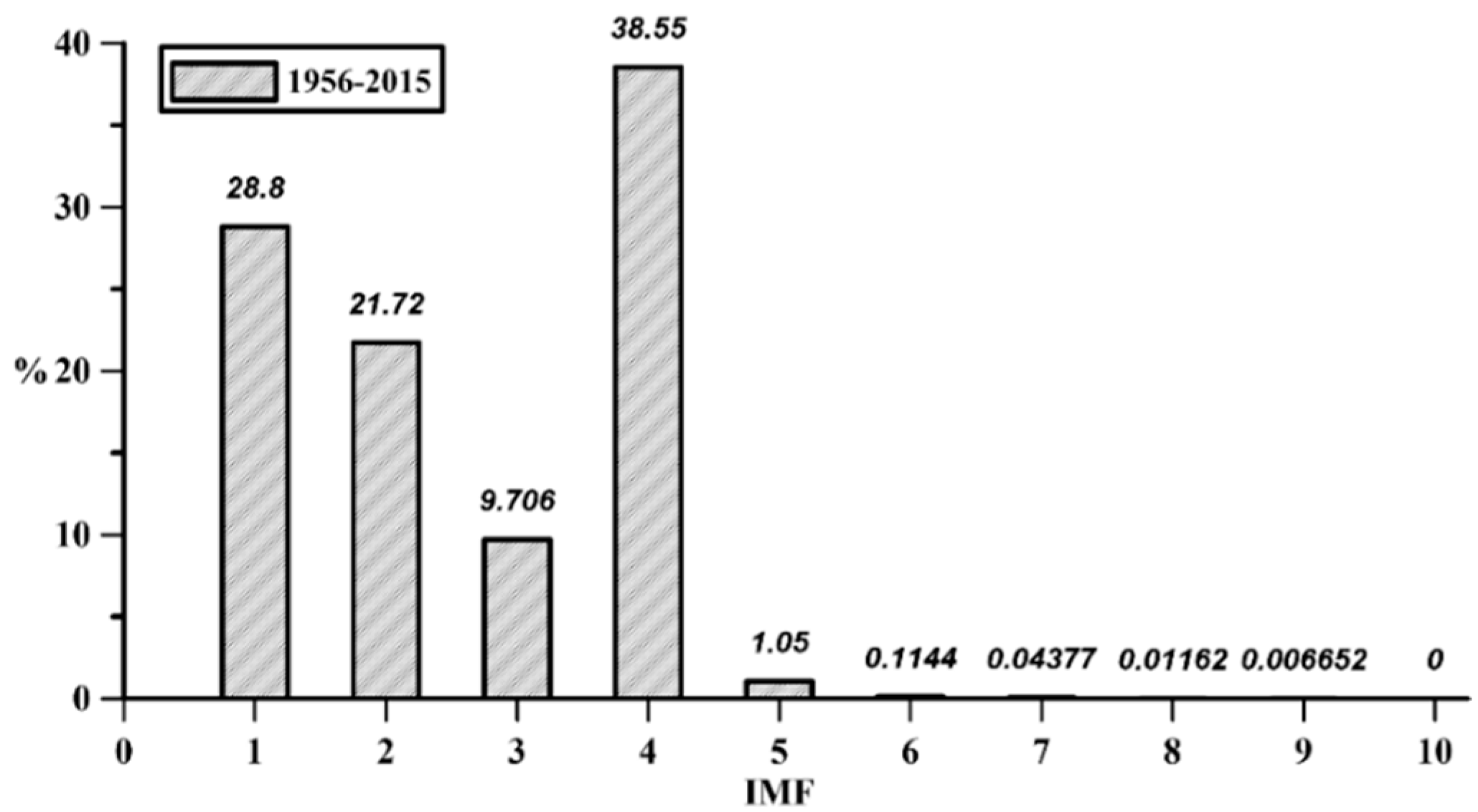
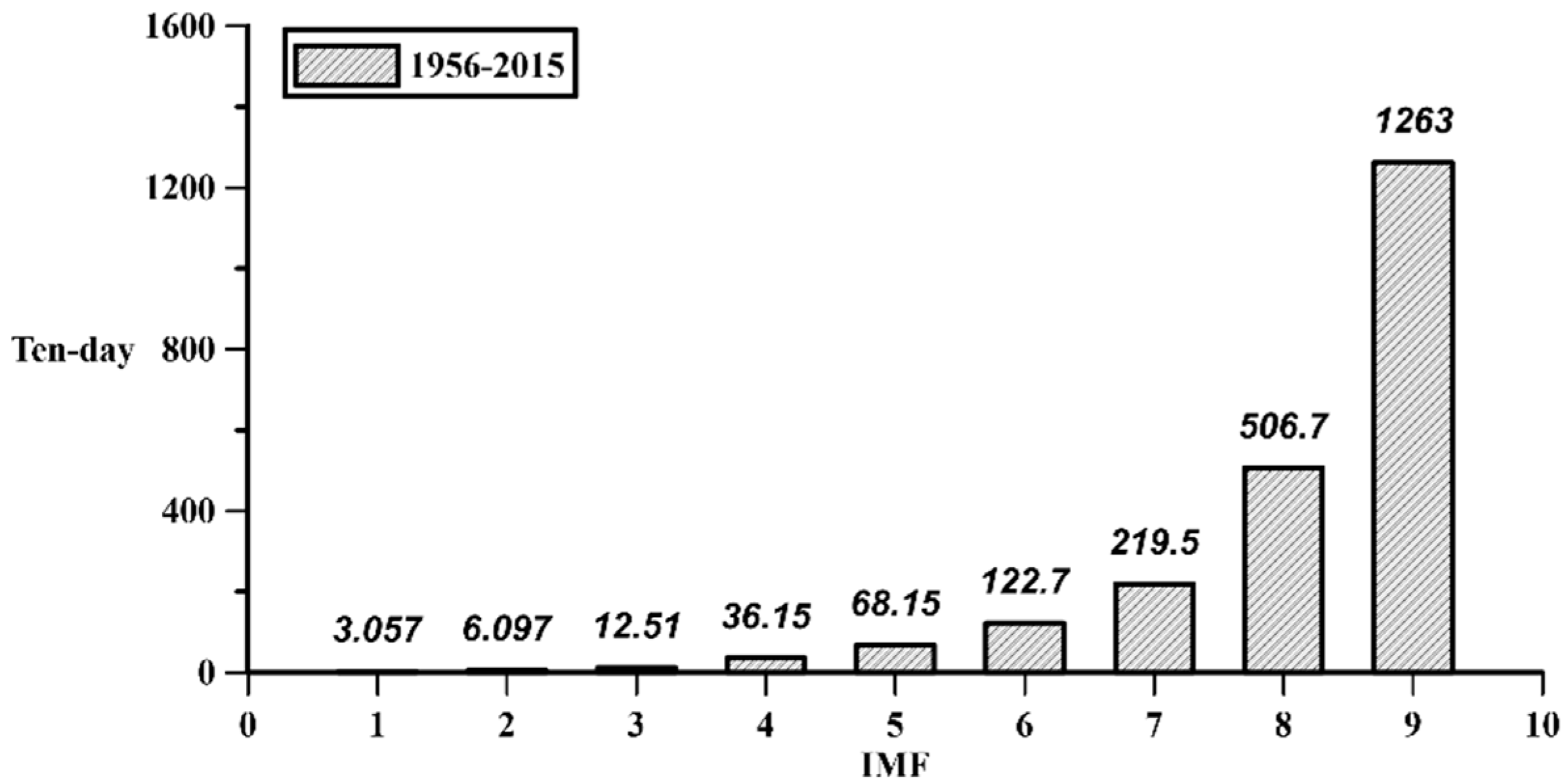
The values of the IMFs decomposed by the EEMD are squared and the sum is taken as the representative value of energy, as shown in Figure 9 and Table 3. After the zero up cross analysis method is used to average the IMF period of each group, the average period represented by the IMF can be obtained. IMF10 is NAN because the period of the sequence cannot get after the zero up cross analysis method.
As can be seen from Figure 9, the energy value is mostly concentrated in IMF4, reaching 39% and the energy of IMF4 is higher than that of other IMFs. Corresponding to IMF4 in Figure 10, it can be found that the corresponding period is about 36 ten-day, which represents that the flow data has a strong annual (36 ten-day) period characteristic. In addition, the IMF1 and IMF2 still have a certain proportion of the energy percentage, which are 29% and 22% respectively, and their periods correspond to about 3 and 6 ten-day, respectively. Therefore, it can be seen that seasonal characteristics exists in the flow data.
3.2. Analysis of 6 Groups of 10-Year Flow Data
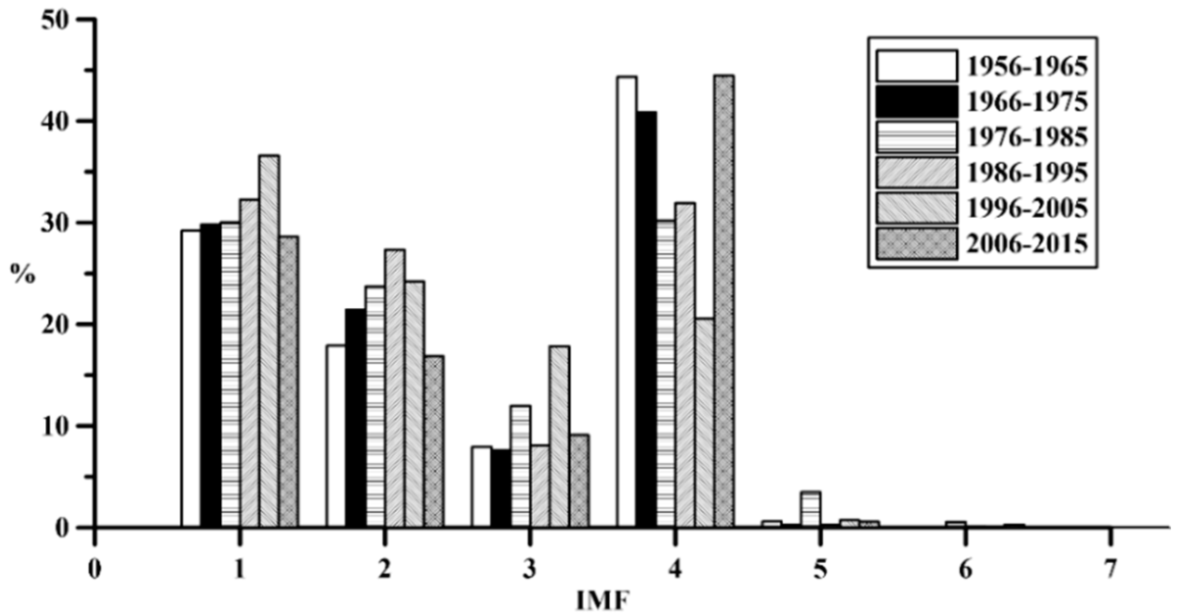
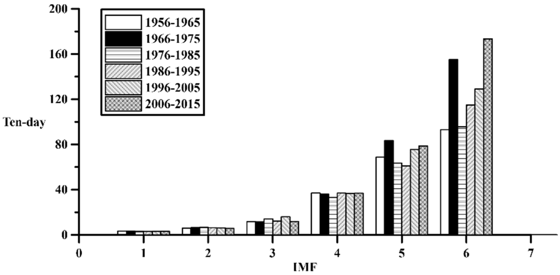
The historical flow data (1956–2015) is divided into 6 decades, and the EEMD screening is implement to get the IMFs and the residue. The relationship between the period, energy, and flow data of different segment IMFs will be discussed. The period and energy percentage distribution of IMFs for each decade are shown in Table 4 and Figure 11 and Figure 12.
The corresponding relationship between the energy percentage of each IMFs and the average period is shown in Figure 11 and Figure 12. We can find the energy distribution concentrates in IMF1–IMF4, which correspond to an average period from 2.96 to 37.03 ten-days. In addition, it can be found that the energy percentage of IMF4 for the 6 groups has the most highest weight, with an average of about 20.5–44.5% compared with total weight of all IMFs, and it corresponds to an average period around 36 ten-days. Moreover, the minor IMFs, IMF1 and IMF2, are have around 28–36% and 18–27% energy of the total respectively, and their corresponding periods are about 3 and 6 ten-days. These results are similar to the 60-year flow analysis, as shown in Table 4.
3.3. Data Synthesis
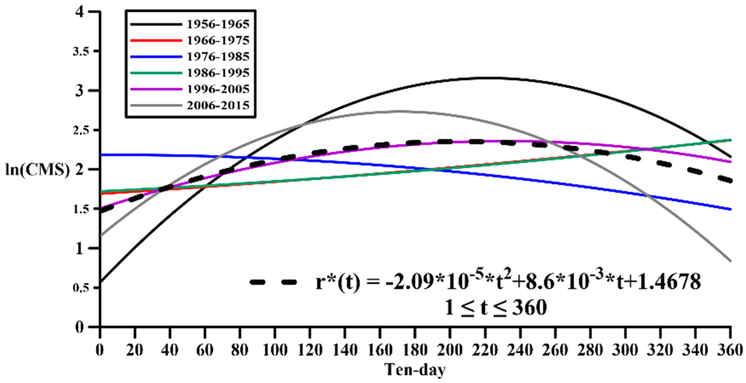
This section explains the synthesis of flow data. The historical flow data (1956–2015) is divided into six groups of 10-year segments in order. After decomposing through EEMD, multiple IMFs and residue corresponding to them can be obtained. The decadal residues are shown in Figure 13. Regression analysis of different residue in each group is fitted to a new residue representing the value.
This study used two methods to synthesize new decadal flow data as the basis for simulation research. Method (I): first permutations and combinations all IMFs to get ni (67 = 279,936) new IMF set. Where n is the number of groups and i is the number of IMFs each group. After permutations and combinations of the IMFs, add a representative value of the residue, which is the regression of six residues. The representative value of the residue is shown in Figure 13, the bold dashed line. Regression analysis fits the representative value of the residue, and then adds this residue to the IMF of the 279,936 group to obtain the synthesis flow data of the 279,936 group for 10 years. Method (II): all the IMFs and the residue in each group are permutations and combinations to obtain a total of ni + 1 (67 + 1 = 1,679,616) new synthetic flow data. In the following, the new flow data synthesized from the two methods and historical flow data are compared with each other, and the differences are explored. In addition, this study will apply new flow data synthesized from two different methods to simulate Hushan reservoir water supply systems, and sequentially discuss the simulation results of different synthetic flow data in different water supply scenarios.
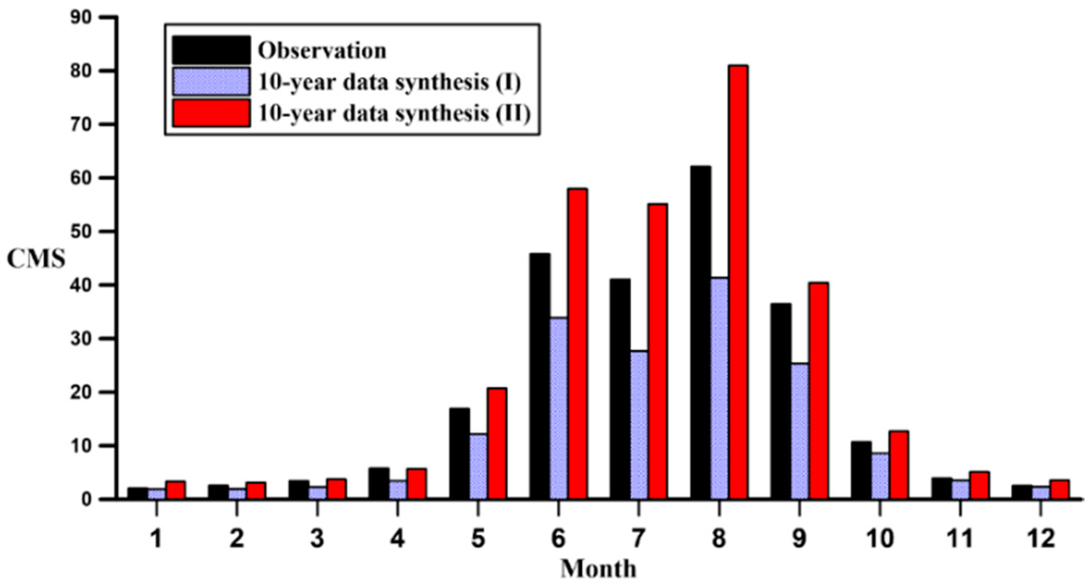
Result of comparing the synthetic data with historical data divided by 10 years is shown in Table 5 and Figure 14. For the historical data, the flow in Qingshui river is significantly different between the wet and dry season; the flow from wet season, May to October, is significantly higher than November to April. The ratio of wet/dry is about 9:1. The highest flow occurs in August (62.09 m3/s) and the lowest flow occurs in January (2.05 m3/s). Compared the historical with the synthetic flow, the monthly distribution is similar between both Method I and Method II. The synthetic flow is concentrated in May–October, and the highest flow always occurs in August, but the lowest flow occurs in the dry season in January and February. In terms of the overall flow during the wet season, the average synthesized by Method I is significantly less than the current situation; in contrast, the average synthesized by Method II is much higher. In the dry season, the average synthesized by Method I and Method II is not much different from the current.
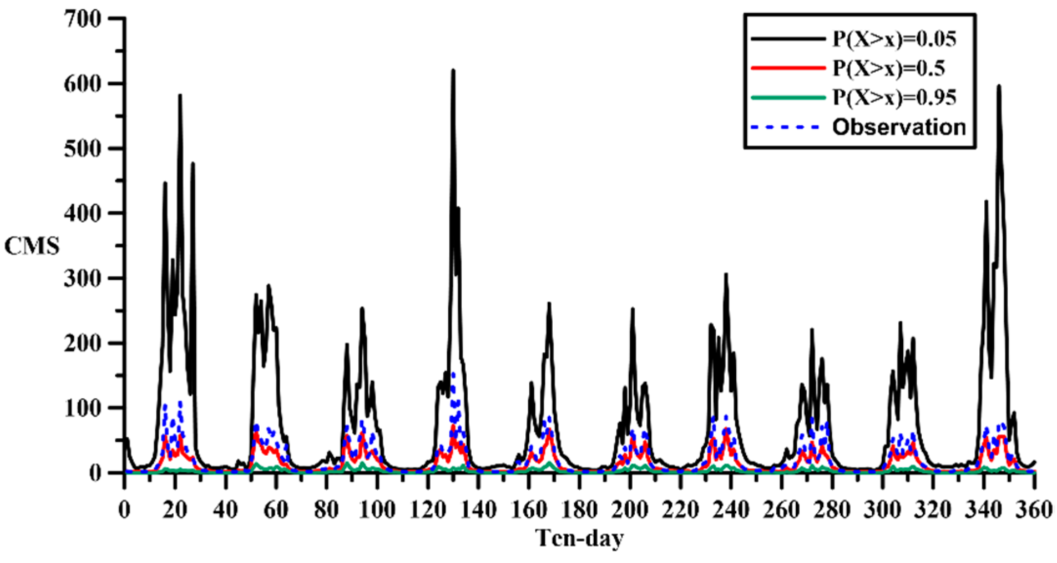
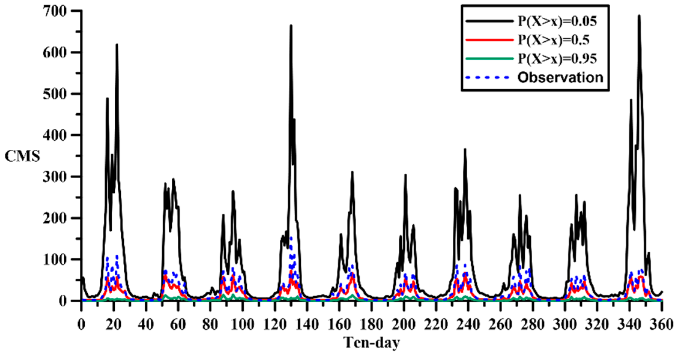
The distribution of the probability of exceedance is shown in the Figure 15 and Figure 16. For the 10-year synthesis, the overall time distribution is consistent with the historical one; furthermore, the synthesis keeps the distribution of wet and dry seasons as well. Through the probability of exceedance of 0.05, the extreme flow of Method II is greater than Method I. In contrast, while the probability of exceedance is 0.95, the flow data of Method II is much less than Method I. This will also lead to the opposite result of the average flow in the simulation of the water supply system.
Although the preceding says that, there are not much variance of the distribution trend between the 10-year flow data synthesized by these two different methods. However, the annual average between two synthesis methods is more significant. The flow data synthesized by Method II has an annual average flow of 24.34 m3/s, which is more than the annual average of Method I, 13.71 m3/s. The water supply system simulation will be based on these three flow sequences, historical data, Method I and Method II synthetic data, to simulate the water supply system of Hushan reservoir.
3.4. Application of Synthesis Data
Next, we apply the synthesized flow data to simulate the water supply system according to the given two demand scenarios. Using the historical flow data, Method I and the Method II synthetic flow data are used for simulation, and the simulation results are shown in the Table 6 and Figure 17.
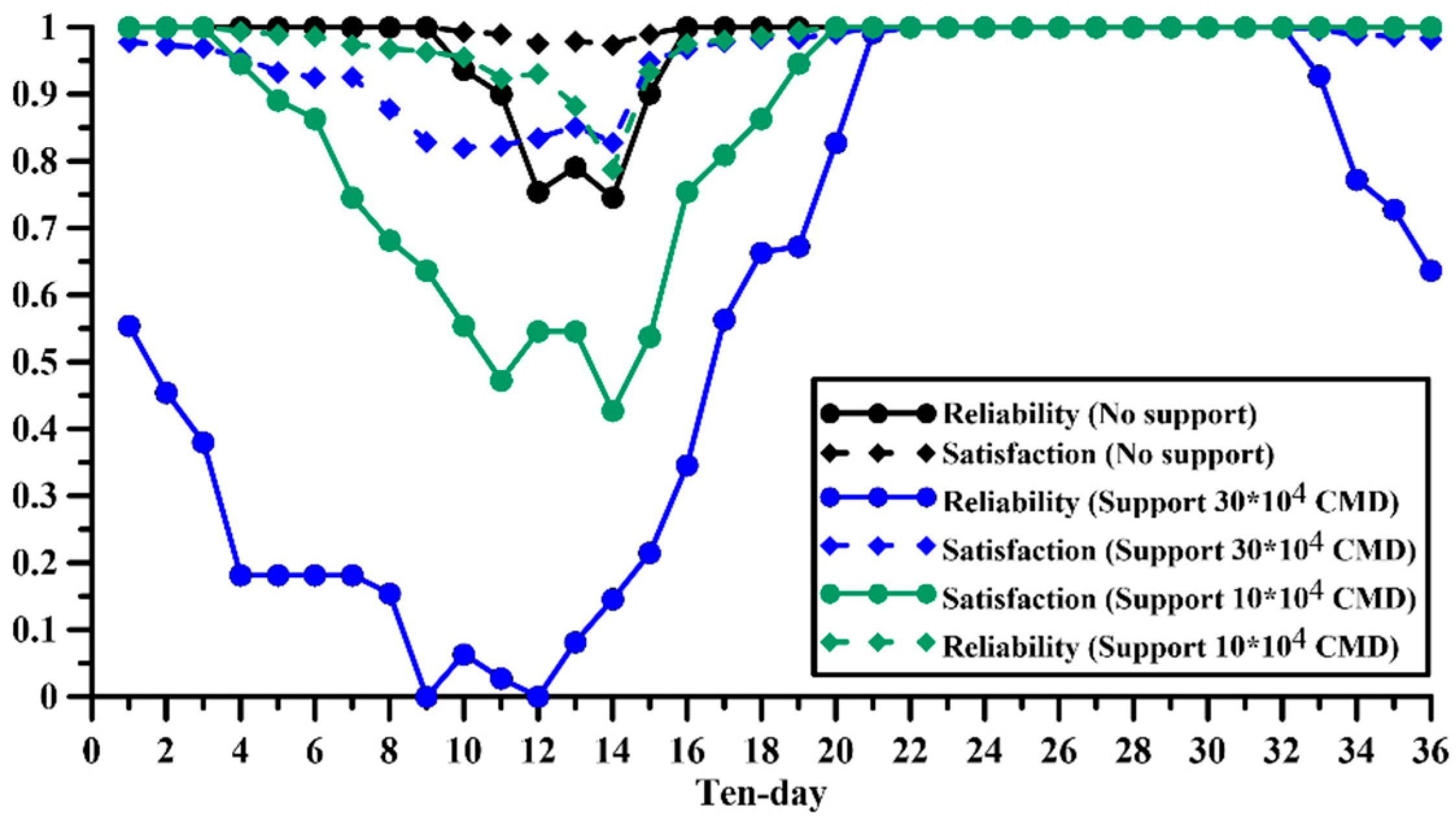
First, we apply the historical flow to simulate the water supply system. For the case of no supporting industrial water in Scenario I, the annual water supply and shortage are 101.93 × 10⁶ m3 and 0.27 × 10⁶ m3, respectively. The water shortage index (SI) is only 0.002. While the water shortage occurring, the average daily water shortage (ADWS) is only 0.03 × 10⁶ m3. The preceding indices show that if the Hushan reservoir only supplies water for domestic demand, the water supply situation will be very stable and shortage will not be easy to occur. In the case of supporting industrial water in Scenario II. If the daily support for industrial water is 300,000 m3, the annual water supply will reach 165.14 × 10⁶ m3, and the annual water shortage will also increase significantly to 9.74 × 10⁶ m3. Although the SI only increases to 0.309, and the ADWS only increases to 0.06 × 10⁶ m3 while the water shortage occurred. The reliability of the water supply reaches 0 already at the 9th and 11th ten-day, as depicted in Figure 17. The result show that the water supply risk in demand Scenario II is relatively severe than Scenario I.
Because the simulation of demand Scenario II indicates severe impact on domestic, we set the domestic SI = 0.1, and try to find the capability of industrial supporting for Hushan reservoir. We found that Hushan reservoir can support 100,000 m3/day of industrial water, and the annual water shortage has decreased to 2.18 × 10⁶ m3. The number of average consecutive dry days (ACDD) for domestic has been greatly reduced to 45 days, and the reliability of the water supply is also raised to 0.4–0.5. In the following analyses, we recommend the daily supporting amount for industry from the Hushan reservoir should be 100,000 m3 as basis.
We simulate the water supply system with the historical flow as applied to method I (279,936 groups) and method II (1,679,616 groups) for newly synthesized flow data. The results are compared based on the ensemble average (as shown in Table 7). Scenario I without considers supporting industrial water, the current annual water supply is 101.93 × 10⁶ m3, the annual water shortage is only 0.27 × 10⁶ m3, and the SI is only 0.002. While the water shortage occurring, the ADWS is only 0.03 × 10⁶ m3.
According to the water supply simulation results of 279,936 sets of flow data in Method I, the annual water supply slightly decreased to 98.25 × 10⁶ m3, the annual water shortage increased to 3.59 × 10⁶ m3, and the SI increased significantly to 0.668. While the water shortage occurring, the ADWS is increased slightly to 0.05 × 10⁶ m3. However, Figure 18 shows that whether the reliability is lower than the current simulation result, they are still above 0.5, the lowest satisfaction is 0.87, which is generally acceptable.
According to the water supply simulation results of 1,679,616 sets of flow data in Method II. The annual water supply decreases to 95.52 × 10⁶ m3, the annual water shortage has increased significantly to 6.68 × 10⁶ m3. The SI increased significantly to 1.96 and the ADWS increased to 0.07 × 10⁶ m3 as well. Figure 18 shows that the reliability is similar to the method I in dry season. However, Method II’s reliability is lower than method I value in the wet season. The satisfaction is generally lower than the current situation and the method I, but the minimum is still 0.84. The water supply situation of Method II is still acceptable. There is something odd: why the average annual flow of Method II is significantly more than the current situation and the average flow of Method I, but the simulation results are worse than the other cases? The main reason is that the extreme flow of the Method II often occurs; excessive flow cannot be used efficiently and there are many low flows during wet season. Therefore, the simulation result of Method II is the worst.
Finally, we simulate the water supply system using the historical flow with Method I and Method II’s synthesis flow data. The results are compared to the ensemble average (as shown in Table 8). Under the condition of supporting 100,000 m3 of industrial demand daily, the current annual water supply is 128.30 × 10⁶ m3, the annual water shortage is 2.18 × 10⁶ m3 and the SI is 0.1. While water shortage occurs, the average daily water shortage is 0.05 × 10⁶ m3.
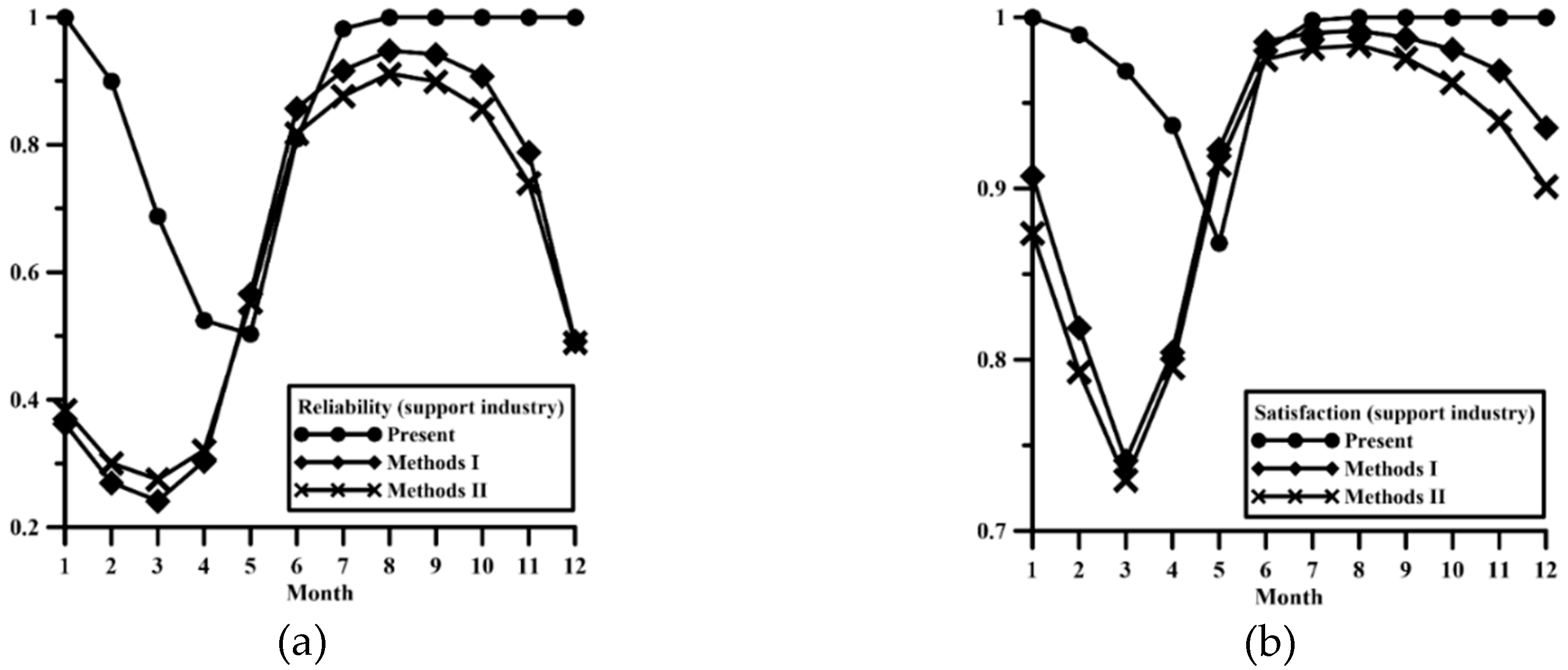
According to the simulation result of water supply in Method I, the annual water supply decreased slightly to 116.82 × 10⁶ m3, the annual water shortage increased to 11 × 106 m3, and the SI increased significantly to 1.203. While the water shortage occurring, the ADWS is still maintained at 0.05 × 10⁶ m3. Figure 19 shows that the reliability decrease more earlier than the current situation, the lowest monthly reliability reaches 0.24 in March, and recoveries in May. The lowest fulfillment of demand still occurs in March (0.74). In terms of dry season, the risk of water supply shortage is much worse than the current situation.
According to the simulation result of water supply in Method II, the annual water supply decreased to 113.82 × 10⁶ m3, the annual water shortage increased sharply to 13.46 × 10⁶ m3, and the SI increased significantly to 2.12. While occurs the water shortage event, the ADWS also increased to 0.07 × 10⁶ m3. Figure 19 depicts that the reliability is similar to but lower than Method I in the dry season. Compared with the current situation, the water shortage occurs earlier, but it is lower than the Method I in the wet season. The satisfaction is generally lower than the current situation and the Method I, but similar to Method I. The satisfaction rises rapidly in May, which is higher than the current simulation results. However, the satisfaction is decreasing from August to October in wet season, it seems worse than the others.
In summary, no matter what kind of water supply scenario is applied, the current results are better than Method I and Method II. Although the simulation result of Method I is similar to Method II, the ensemble result of Method I is slightly better than the Method II. However, Method II synthesis annual average flow is significantly more than the current flow and the Method I flow, but the simulation results are worse than other cases. The main reason is that the extreme flow of the method II often occurs. Excessive flow cannot be used efficiently and there are many low flows in wet season. Therefore, the simulation result of Method II is the worst.
4. Conclusions
The IMFs and residue of the Tongtou weir flow data can be obtained by EEMD decomposition. This method can effectively solve the stationary or nonstationary impacts of hydrological data due to climate change. In this study, two methods are used to synthesize new 10-year flow series data. Method I uses the IMFs segmented data to reorganize the periodic characteristics and sums them up with the residue representation; in contrast, Method II uses the permutation and combination of all IMFs and residues. The new synthetic flow data will provide the input of simulation for the Hushan Reservoir water supply system.
In the energy distribution of IMFs, most of the energy is concentrated between IMF1 and IMF4, which IMF4 has the largest weight (39%), and the corresponding period is about 36 ten-day periods (1 year). However, IMF1 still has a certain proportion of energy percentage, the corresponding period is about 3 ten-day periods (1 month). This reflects that the flow of Tongtou weir is not only affected by a 1-year periodic sequence, but influenced by the monthly rainfall event. Comparing the current situation with the new data generated by EEMD, the generated data is similar to the current flow distribution, but the flow distribution during the wet season is significantly different (±0.63 m3/s), and the flow difference during the dry season is insignificant (±0.78 m3/s).
For the Scenario I without considers supporting industrial water, the simulation results of the generation data of Method I show that compared with the current situation, the SI has increased significantly from 0.002 to 0.668, and the number of ACDD of water shortage has also increased significantly from 9 to 51.2 days. The simulation results of Method II show that the SI is more severe than the current situation and Method I, it reaches 1.96. The number of ACDD increased slightly to 59.28 days. In addition, it can be found from the reliability and satisfaction Figure that the simulation results of the synthesis flow in this study will occur water shortages earlier than the current situation.
Scenario II considers supporting industrial water usage, the simulation results of Method I show that the SI has increased significantly to 1.023, and the number of ACDD of water shortage has also increased significantly to 111 days. The simulation results of Method II show that the SI is more severe to 2.12. The number of ACDD increased slightly to 113.82 days. In addition, it can be found from the reliability and satisfaction figure that no matter in which way the synthesis flow is simulated, supporting industrial water will seriously affect the equity of domestic water.
In this study, the multiplication data obtained through permutation and combination after EEMD can show the flow distribution characteristics of the Tongtou weir. In the future, the hydrological factors, such as temperature and rainfall in the same area, can be integrated to explore the correlation between the overall hydrological factors.
Author Contributions
T.-Y.C. analyzed the data and drafted the manuscript; W.-C.H. revised the manuscript. All authors have read and agreed to the published version of the manuscript.
Funding
This research received no external funding.
Acknowledgments
This research was sponsored by the Ministry of Science and Technology in Taiwan (MOST 106-2625-M-019-001).
Conflicts of Interest
The authors declare no conflict of interest.
References
- Huang, N.E.; Shen, Z.; Long, S.R. A new view of nonlinear water waves: The hilbert spectrum. Annu. Rev. Fluid Mech. 1999, 31, 417–457. [Google Scholar] [CrossRef] [Green Version]
- Huang, N.E.; Shen, Z.; Long, S.R.; Wu, M.C.; Shih, H.H.; Zheng, Q.; Yen, N.C.; Tung, C.C.; Liu, H.H. The empirical mode decomposition and the Hilbert spectrum for nonlinear and nonstationary time series analysis. Proc. R. Soc. Math. Phys. 1998, 454, 903–995. [Google Scholar] [CrossRef]
- Yang, Y.Z. The Application of Empirical Mode Decomposition on the SASW; National Cheng Kung University: Tainan, Taiwan, 2008. [Google Scholar]
- Huang, Y.; Schmitt, F.G.; Lu, Z.; Liu, Y. Analysis of daily river flow fluctuations using empirical mode decomposition and arbitrary order Hilbert spectral analysis. J. Hydrol. 2009, 373, 103–111. [Google Scholar] [CrossRef] [Green Version]
- Wu, Z.H.; Huang, N.E. On the filtering properties of the empirical mode decomposition. Adv. Adapt. Data Anal. 2010, 2, 397–414. [Google Scholar] [CrossRef]
- Lu, K.Y. Use EMD to Study the ISO in the Background Circulation of the Typhoon Morakot; National Central University: Taoyuan, Taiwan, 2011. [Google Scholar]
- Lee, T.; Ouarda, T. Prediction of climate nonstationary oscillation processes with empirical mode decomposition. J. Geophys. Res. Atmos. 2011, 116, D06107. [Google Scholar] [CrossRef] [Green Version]
- Lee, T.; Uarda, T. Stochastic simulation of nonstationary oscillation hydroclimatic processes using empirical mode decomposition. Water Resour. Res. 2012, 48, W02514. [Google Scholar] [CrossRef] [Green Version]
- Molla, M.K.I.; Rahman, M.S.; Sumi, A.; Banik, P. Empirical Mode Decomposition Analysis of climate changes with Special Reference to Rainfall Data. Discret. Dyn. Nat. Soc. 2006, 2006, 1–17. [Google Scholar] [CrossRef] [Green Version]
- Molla, M.K.I.; Sumi, A.; Rahman, M.S. Analysis of Temperature Change under Global Warming Impact using Empirical Mode Decomposition. Int. J. Inf. Tecnol. 2007, 3, 131–139. [Google Scholar]
- Huang, S.Z.; Chang, J.X.; Huang, Q.; Chen, Y.T. Monthly streamflow prediction using modified EMD-based support vector machine. J. Hydrol. 2014, 511, 764–775. [Google Scholar] [CrossRef]
- Meng, E.H.; Huang, S.Z.; Huang, Q.; Fang, W.; Wu, L.Z.; Wang, L. A robust method for non-stationary streamflow prediction based on improved EMD-SVM model. J. Hydrol. 2019, 568, 462–478. [Google Scholar] [CrossRef]
- Zhang, H.B.; Wang, B.; Lan, T.; Chen, K. A modified method for non-stationary hydrological time series forecasting based on empirical mode decomposition. J. Hydroelectr. Eng. 2015, 34, 42–53. [Google Scholar]
- Wu, Z.H.; Huang, N.E. Ensemble empirical mode decomposition: A noise-assisted data analysis method. Adv. Adapt. Data Anal. 2005, 1, 1–41. [Google Scholar] [CrossRef]
- Zhao, X.H.; Chen, X. Auto Regressive and Ensemble Empirical Mode Decomposition Hybrid Model for Annual Runoff Forecasting. Water Resour. Manag. 2015, 29, 2913–2926. [Google Scholar] [CrossRef]
- Zhang, X.; Zhang, Q.W.; Zhang, G.; Nie, Z.P.; Gui, Z.F. A Hybrid Model for Annual Runoff Time Series Forecasting Using Elman Neural Network with Ensemble Empirical Mode Decomposition. Water 2018, 10, 416. [Google Scholar] [CrossRef] [Green Version]
- Bai, L.; Xu, J.H.; Chen, Z.S.; Li, W.H.; Liu, Z.H.; Zhao, B.F.; Wang, Z.J. The regional features of temperature variation trends over Xinjiang in China by the ensemble empirical mode decomposition method. Int. J. Climatol. 2015, 35, 3229–3237. [Google Scholar] [CrossRef]
- Yu, Y.H.; Zhang, H.B.; Singh, V.P. Forward Prediction of Runoff Data in Data-Scarce Basins with an Improved Ensemble Empirical Mode Decomposition (EEMD) Model. Water 2018, 10, 388. [Google Scholar] [CrossRef] [Green Version]
- Bai, Y.; Wang, P.; Xie, J.J.; Li, J.T.; Li, C.A. Additive Model for Monthly Reservoir Inflow Forecast. J. Hydrol. Eng. 2015, 20, 04014079. [Google Scholar] [CrossRef]
- Yeh, W.W.-G. Reservoir management and operations models: A state-of-the-art review. Water Resour. Res. 1985, 21, 1797–1818. [Google Scholar] [CrossRef]
- Wurbs, R.A. Reservoir-System Simulation and Optimization Model. J. Water Resour. Plan. Manag. 1993, 119, 455–472. [Google Scholar] [CrossRef]
- Chang, J.X.; Wang, Y.M.; Huang, Q. Reservoir Systems Operation Model Using Simulation and Neural Network. In Proceedings of the Second IFIP Conference on Artificial Intelligence Applications and Innovations, Beijing, China, 7–9 September 2005. [Google Scholar]
- Lin, N.M.; Rutten, M. Optimal Operation of a Network of Multi-purpose Reservoir: A Review. Procedia Eng. 2016, 154, 1376–1384. [Google Scholar] [CrossRef] [Green Version]
- Lee, J.L.; Huang, W.C. Climate change impact assessment on Zhoshui River water supply in Taiwan. Terr. Atmos. Ocean. Sci. 2017, 28, 463–478. [Google Scholar] [CrossRef] [Green Version]
- Lee, J.L.; Huang, W.C. Impact on Water Utilization of Zhoshui River Basin by Wushe Reservoir Sediment and Hushan Reservoir Operation. Taiwan Water Conserv. 2012, 60, 85–97. [Google Scholar]
- Chu, T.Y.; Huang, W.C. Water-Resource Utilization of Hushan Reservoir in Taiwan. Taiwan Water Conserv. 2016, 64, 1–11. [Google Scholar]
- Huang, W.C.; Chu, T.Y.; Jang, Y.S.; Lee, J.L. Data Synthesis Based on Empirical Mode Decomposition. J. Hydrol. Eng. 2020. accepted. [Google Scholar]
- Goda, Y. Effect of Wave Tilting on Zero-Crossing Wave Heights and Periods. Coast. Eng. Jpn. 1986, 29, 79–90. [Google Scholar] [CrossRef]
- Goda, Y. Random Seas and Design of Maritime Structures, 1st ed.; Yokohama National University: Yokohama, Japan, 1985. [Google Scholar]
- Tong, C.H. A Suitability Study on 2-D Irregular Wave Tests; National Taiwan Ocean University: Keelung, Taiwan, 2013. [Google Scholar]
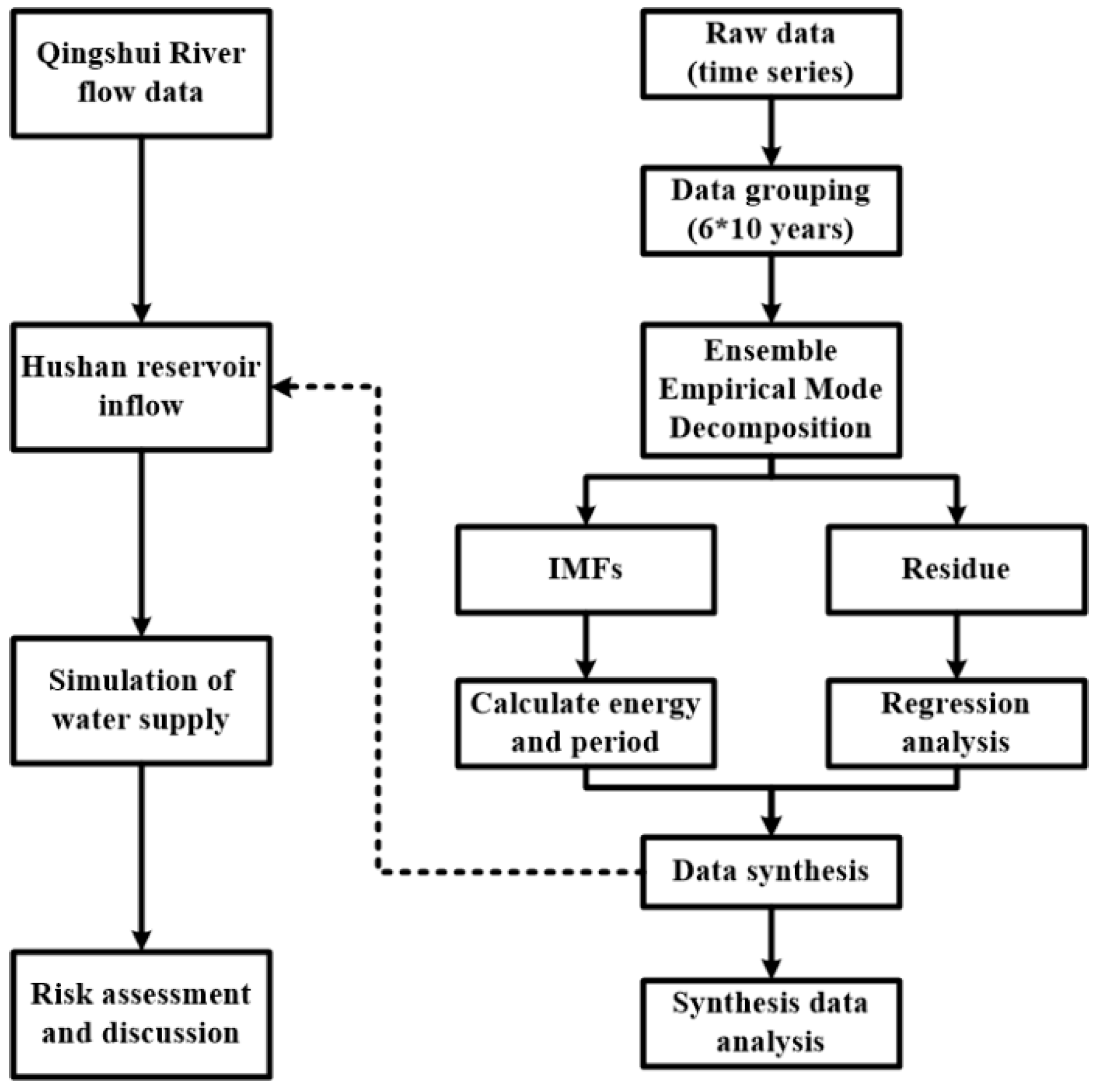
Figure 1.
Research flowchart. EMD, empirical mode decomposition components.

Figure 2.
Location of study area.

Figure 3.
Results of EMD (empirical mode decomposition) method decomposition.

Figure 4.
Show of the zero up-cross method [30]. H, The wave high; nmax: The average value of the highest point (peak).
Figure 4.
Show of the zero up-cross method [30]. H, The wave high; nmax: The average value of the highest point (peak).

Figure 5.
Graphs of the data synthesis process. h: segment.

Figure 6.
Water supply system of Hushan reservoir.

Figure 7.
Program simulation flowchart.

Figure 8.
Decomposition of 60-year flow data by EMD.

Figure 9.
Weight of each IMF for a 60-year flow.

Figure 10.
Average period of each IMF for a 60-year flow.

Figure 11.
Weight of each IMF for a 10-year flow.

Figure 12.
Average period of each IMF for a 10-year flow.

Figure 13.
Flow data residues and their representative equation. CMS, m3/s; r*(t): representative values of the residue.
Figure 13.
Flow data residues and their representative equation. CMS, m3/s; r*(t): representative values of the residue.

Figure 14.
Comparisons of 10-year flow data.

Figure 15.
Comparisons of 10-year flow data with Method I. P(X > x): probability of exceedance.

Figure 16.
Comparisons of 10-year flow data with Method II.

Figure 17.
Ten-day reliability and satisfaction of the water supply in present each scenario. CMD, m3/day.
Figure 17.
Ten-day reliability and satisfaction of the water supply in present each scenario. CMD, m3/day.

Figure 18.
Monthly (a) reliability and (b) satisfaction of the water supply for Scenario I.

Figure 19.
Monthly (a) reliability and (b) satisfaction of the water supply for Scenario II.


Table 1.
Elevation-area-capacity relationship of Hushan reservoir.
| Water Level (m) | Area (ha) | Volume (104 m3) |
|---|---|---|
| Dead water level: 165 | 12 | 36 |
| 170 | 32 | 147 |
| 175 | 76 | 418 |
| 180 | 99 | 857 |
| 185 | 107 | 1371 |
| 190 | 132 | 1969 |
| 195 | 142 | 2653 |
| 200 | 170 | 3432 |
| 205 | 181 | 4310 |
| 210 | 210 | 5288 |
| Full water level: 211.5 | 214 | 5612 |
Table 2.
Scenario description.
| Scenario | I | II |
|---|---|---|
| Water supply range | Supply the domestic water | Support the industrial water |
| The operational regulations | The upper and lower rule was set at the water level of 190 and 185 m in Hushan reservoir, respectively. | |
Table 3.
Results of 60-year data by EMD with energy and period.
| IMF | 1 | 2 | 3 | 4 | 5 | 6 | 7 | 8 | 9 | 10 |
|---|---|---|---|---|---|---|---|---|---|---|
| Energy (%) | 29% | 22% | 10% | 39% | 1% | 0% | 0% | 0% | 0% | 0% |
| Period (ten-day) | 3.06 | 6.10 | 12.51 | 36.15 | 68.15 | 122.69 | 219.52 | 506.72 | 1262.74 | N/A |
Table 4.
Results of decadal data by EMD with energy and period.
| Energy and Period of Each IMFs Title | 1956–1965 | 1966–1975 | 1976–1985 | 1986–1995 | 1996–2005 | 2006–2015 | |
|---|---|---|---|---|---|---|---|
| IMF1 | Energy (%) | 29.21 | 29.80 | 30.01 | 32.27 | 36.61 | 28.63 |
| Period (ten-day) | 3.34 | 3.39 | 3.04 | 2.96 | 3.05 | 3.18 | |
| IMF2 | Energy (%) | 17.89 | 21.43 | 23.75 | 27.34 | 24.22 | 16.89 |
| Period (ten-day) | 5.89 | 6.38 | 6.79 | 6.29 | 6.17 | 5.72 | |
| IMF3 | Energy (%) | 7.94 | 7.57 | 11.98 | 8.09 | 17.82 | 9.12 |
| Period (ten-day) | 11.80 | 11.48 | 14.16 | 12.28 | 15.97 | 11.87 | |
| IMF4 | Energy (%) | 44.32 | 40.85 | 30.22 | 31.93 | 20.54 | 44.46 |
| Period (ten-day) | 37.03 | 35.97 | 33.00 | 36.98 | 36.78 | 36.90 | |
| IMF5 | Energy (%) | 0.60 | 0.31 | 3.47 | 0.28 | 0.72 | 0.59 |
| Period (ten-day) | 68.73 | 83.47 | 63.53 | 61.08 | 75.53 | 78.63 | |
| IMF6 | Energy (%) | 0.04 | 0.04 | 0.56 | 0.10 | 0.09 | 0.31 |
| Period (ten-day) | 93.06 | 155.07 | 95.69 | 114.80 | 129.14 | 173.41 | |
| IMF7 | Energy (%) | 0.00 | 0.00 | 0.00 | 0.00 | 0.00 | 0.00 |
| Period (ten-day) | - | - | - | - | - | - | |
Table 5.
Comparison of historical and synthesis flow data.
| Month | 1 | 2 | 3 | 4 | 5 | 6 | 7 | 8 | 9 | 10 | 11 | 12 | Average | |
|---|---|---|---|---|---|---|---|---|---|---|---|---|---|---|
| Flow (cms) | ||||||||||||||
| Observation | 2.05 | 2.56 | 3.39 | 5.74 | 16.85 | 45.82 | 41.02 | 62.09 | 36.43 | 10.67 | 3.88 | 2.55 | 19.24 | |
| Synthesis (I) | 1.91 | 1.98 | 2.28 | 3.44 | 12.17 | 33.89 | 27.69 | 41.37 | 25.33 | 8.59 | 3.54 | 2.33 | 13.71 | |
| Synthesis (II) | 3.29 | 3.10 | 3.70 | 5.67 | 20.70 | 57.92 | 55.11 | 80.93 | 40.40 | 12.68 | 5.08 | 3.54 | 24.34 | |
Table 6.
Indices of the water supply for present.
| Simulation Results | ||||
|---|---|---|---|---|
| Unit: Quantity of Water in 106 m3/yr | ||||
| Present | ||||
| Scenario | No Support Industrial Water | Support Industrial Water (30 × 104 CMD) | Support Industrial Water (10 × 104 CMD) | |
| Project | ||||
| Reservoir supply | 101.93 | 165.14 | 128.30 | |
| Domestic shortage | 0.27 | 9.74 | 2.18 | |
| Reservoir inflow | 101.90 | 162.80 | 128.05 | |
| Domestic SI | 0.002 | 0.309 | 0.10 | |
| Reservoir efficiency | 1.91 | 3.09 | 2.40 | |
| Public ACDD | 9.00 | 135.00 | 45.00 | |
| ADWS during water shortage events | 0.03 | 0.06 | 0.05 | |
Note: CMD, m3/day; ACDD, average consecutive dry days; ADWS, average daily water shortage.
Table 7.
Comparison of historical and synthesis flow data. SI, Shortage Index.
| Simulation Results | ||||
|---|---|---|---|---|
| Unit: Quantity of Water in 106 m3/yr | ||||
| No Support Industrial Water | ||||
| Scenario | Present | Method I | Method II | |
| Project | ||||
| Reservoir supply | 101.93 | 98.25 | 95.52 | |
| Domestic shortage | 0.27 | 3.95 | 6.68 | |
| Reservoir inflow | 101.90 | 94.72 | 92.07 | |
| Domestic SI | 0.002 | 0.668 | 1.96 | |
| Reservoir efficiency | 1.91 | 1.84 | 1.79 | |
| Domestic ACDD | 9.00 | 51.2 | 59.28 | |
| ADWS during water shortage events | 0.03 | 0.05 | 0.07 | |
Table 8.
Comparison of historical and synthesis flow data.
| Simulation Results | ||||
|---|---|---|---|---|
| Unit: Quantity of Water in 106 m3/yr; | ||||
| Support Industrial Water (10 × 104 m3/s) | ||||
| Scenario | Present | Method I | Method II | |
| Project | ||||
| Reservoir supply | 128.30 | 116.92 | 113.82 | |
| Public shortage | 2.18 | 11.00 | 13.46 | |
| Reservoir inflow | 128.05 | 112.37 | 109.43 | |
| Public SI | 0.10 | 1.203 | 2.12 | |
| Reservoir efficiency | 2.40 | 2.19 | 2.13 | |
| Public ACDD | 45.0 | 111.0 | 113.82 | |
| ADWS during water shortage events | 0.05 | 0.05 | 0.07 | |
© 2020 by the authors. Licensee MDPI, Basel, Switzerland. This article is an open access article distributed under the terms and conditions of the Creative Commons Attribution (CC BY) license (http://creativecommons.org/licenses/by/4.0/).
Share and Cite
MDPI and ACS Style
Chu, T.-Y.; Huang, W.-C. Application of Empirical Mode Decomposition Method to Synthesize Flow Data: A Case Study of Hushan Reservoir in Taiwan. Water 2020, 12, 927. https://doi.org/10.3390/w12040927
AMA Style
Chu T-Y, Huang W-C. Application of Empirical Mode Decomposition Method to Synthesize Flow Data: A Case Study of Hushan Reservoir in Taiwan. Water. 2020; 12(4):927. https://doi.org/10.3390/w12040927
Chicago/Turabian StyleChu, Tai-Yi, and Wen-Cheng Huang. 2020. "Application of Empirical Mode Decomposition Method to Synthesize Flow Data: A Case Study of Hushan Reservoir in Taiwan" Water 12, no. 4: 927. https://doi.org/10.3390/w12040927
Note that from the first issue of 2016, this journal uses article numbers instead of page numbers. See further details here.