Temporal and Spatial Characteristics of Multidimensional Extreme Precipitation Indicators: A Case Study in the Loess Plateau, China

1
Institute for Energy, Environment and Sustainability Research, UR-NCEPU, North China Electric Power University, Beijing 102206, China
2
Center for Energy, Environment and Ecology Research, UR-BNU, Beijing Normal University, Beijing 100875, China
3
Department of Civil and Environmental Engineering, Brunel University, London, Uxbridge, Middlesex UB8 3PH, UK
*
Author to whom correspondence should be addressed.
Water 2020, 12(4), 1217; https://doi.org/10.3390/w12041217
Submission received: 30 March 2020
/
Revised: 14 April 2020
/
Accepted: 23 April 2020
/
Published: 24 April 2020
(This article belongs to the Special Issue Water Environmental System Analysis)
Abstract
:Extreme precipitation can seriously affect the ecological environment, agriculture, human safety, and property resilience. A full-scale and scientific assessment in extreme precipitation characteristics is necessary for water resources management and providing decision-making support to mitigate the potential losses brought by extreme precipitation. In the present study, a multidimensional risk assessment framework is developed to investigate the spatial–temporal changes in different extreme precipitation indicators. The Gaussian mixture model (GMM) is applied to fit the distribution for each indicator and carry out single index risk assessment. The joint probabilistic features of multiple extreme indicators can be explored through coupling the GMM distributions into copulas. In addition, the moving window approach and the Mann–Kendall test are integrated to examine non-stationary risks (evaluated by “AND”, “OR”, and Kendall return periods) of multidimensional indicators along with their changing trends and significance. The proposed assessment framework is applied to the Loess Plateau, China. Four extreme precipitation indicators are characterized: the amount (P95), the number of days (D95), the intensity (I95), and the proportion (R95) of extreme precipitation. The spatial–temporal changes of these indicators and their multidimensional combinations (including six two-dimensional and three three-dimensional combinations) are fully identified and quantitatively evaluated.
1. Introduction
In recent years, the increasingly catastrophic impact of hydrometeorological disasters has aroused public concern over extreme events due to climate change [1,2,3]. The drastic changes in the global water cycle may lead to increasing extremes such as extreme precipitation and drought in local areas [4,5]. The extreme precipitation can seriously affect eco-environment, agriculture, human safety, and property resilience [6,7,8]. Risk analysis for extreme precipitation is important for hydrologic designs and environmental systems management [9,10,11]. In the process of climate change, the spatial–temporal distribution of precipitation has also changed significantly in many regions around the world. The characteristics of extreme precipitation have also presented dynamic features [12], in which the changes of magnitude or/and frequency of extreme precipitation may have significant impacts on local flooding [10,13]. However, the commonly used risk assessment techniques with stationary assumption (constant probability) make the resulting hydrologic design questionable under changing environmental conditions [10]. Therefore, it is necessary to conduct an in-depth study on the non-stationary risk characteristics of extreme precipitation under climate change. Such research is remarkably valuable to enhance scientific understanding of the possible changes in floods and other secondary disasters, and provide key information for generating appropriate adaptation measures.
A variety of indicators are employed to characterize the duration, intensity, and amount of extreme precipitation [14,15,16,17]. Frequency characteristics estimated from probability distribution functions are often used to assess risks of those extreme precipitation indicators [18,19]. For example, based on the generalized extreme value theory [20] and the moving window approach, Ghosh et al. [21] have explored the non-stationary frequency characteristics of annual maximum rainfall in India. It is worthy to notice that the extreme precipitation indexes are usually correlated among each other, and univariate estimation of the extreme precipitation indicators may underestimate or overestimate the severity of the extreme event [11,15]. The joint probabilistic characteristics of correlated indicators of extreme precipitation are of great importance in hydrological risk management, and have also become essential factors under consideration for water resources planning, design, and management [11].
As a widely accepted and applied multidimensional joint analysis method, the copula method has been successfully applied in hydrological risk assessment [22,23,24]. Two prominent advantages of this method are that the marginal and joint distributions for indicators can be built separately, giving flexibility in choosing different marginal and dependence models, and there are a number of marginal distributions and copula functions available. Particularly, the bivariate copula functions have already been introduced into two-dimensional extreme precipitation studies, and different kinds of return periods (e.g., “AND”, “OR” return periods, see Section 3) are applied to analyze the joint risk characteristics of extreme precipitation indicators (see, e.g., in [15,25]). For instance, Liu et al. [26] have used the copula method to study the joint probabilistic features of six extreme precipitation indicators in southwestern China. Based on projections from climate models, Goswami et al. [15] have applied the copula method to assess the bivariate behaviors of seven extreme indicators in the North Sikkim in the future. Li et al. [11] have incorporated non-stationary analysis into a bivariate analysis of extreme precipitation by using the Archimedean copulas combined with a moving window scheme. The Akaike’s information criteria (AIC, [27]) and Kolomogorov–Smirnov test (KS) were usually employed to do the goodness-of-fit assessment for the copulas [15,16].
Although joint risk analysis of extreme precipitation indicators has been carried out by numerous studies, some challenges still need to be further addressed: (i) Different marginal distributions have been used in previous studies, which may produce noticeable uncertainty, and thus it is desired to adopt a widely applicable marginal distribution to eliminate or reduce model uncertainty. (ii) Bivariate behaviors of extreme precipitation indicators have been extensively characterized, but there are few studies on high-dimensional extremes larger than two, and also no comprehensive analysis on combinations of multiple-dimensional indicators. (iii) The joint return periods are frequently characterized by “AND” and “OR” types, which can hardly meet the needs of multivariate risk assessments in practical application. Moreover, no research in this field (extreme precipitation) is found to address the high-dimensional Kendall return period. Further, the vine copula, which is built by decomposed bivariate copulas, has been used to construct multivariate joint distributions in recent years [28]. However, for the three-dimensional cases, the parametric copula functions, such as Archimedean and elliptical copula families, are easy to calculate and are effective to capture the dependence structure among the variables [29,30].
The challenges mentioned above prompt us to propose a comprehensive risk assessment framework, which can extensively evaluate the spatial–temporal changes of multidimensional extreme precipitation indicators. Therefore, the main purpose of this study is to achieve the following objectives. (i) Adopting a marginal distribution which can be applied uniformly for all indicators. (ii) Assessing the risks of multidimensional indicator combinations by different types of return periods, including two- and three-dimensional Kendall return periods. (iii) Establishing a non-stationary assessment model and evaluate the spatial–temporal changing features of risks for multidimensional indicators.
2. Overview of the study area and data
With an area of ~640,000 km2, the Loess Plateau, which is located in the north of central China, is selected as the study area (Figure 1). The altitude of the Loess Plateau mainly ranges between 900 to 2200 m, and the terrain is characterized by high-west and low-east patterns. In the Loess Plateau, there are some mountains up to 3500 m above sea level, as well as plains and basins at an altitude of only 400 to 500 m. The Loess Plateau is also the largest area covered by loess in the world, presenting loose soil structure and fragile eco-environmental systems.
The average annual precipitation in the Loess Plateau is only 413.6 mm. Due to the influence of monsoon climate and complex geomorphic types, the precipitation in the Loess Plateau varies greatly in time and space. The spatial distribution shows more precipitation in the southeast and less in the northwest (Figure 1b). From southeast to northwest, the climate successively presents semi-humid, semi-arid, and arid types. The temporal distribution of precipitation in the Loess Plateau is also uneven. This mainly contains two aspects: First, the inter-annual variability of precipitation is noticeable. In the years with excessive rainfall, the precipitation may be several times more than that in the water-deficient years. Second, seasonal differences in precipitation are also large, with precipitation in Summer and Autumn accounting for 60–80% of the annual precipitation. The precipitation in rainy season may be concentrated in few intensive rainfall events. It is customary that a single rainstorm accounts for 30% or more of the annual rainfall, leading to coexistence of water shortage and soil erosion in the Loess Plateau.
The daily precipitation data with time period from 1959 to 2018 of 63 stations (Figure 1b, two of them are located near the Loess Plateau) are collected from the China Meteorological Administration. The ratio of missing values over all stations is from 1.23% to 3.15%, with an average of 1.83%, and the proportion of missing values in rainy season (July–September) is 0.44% on average. The missing values were replaced by average precipitation of neighboring stations, and the calculation of extreme indicators would be affected very little [31]. In order to facilitate the comparative study of the multidimensional risks of extreme precipitation indicators in different climatic regions, the study area is divided into two sub-regions based on the rainfall pattern (400 mm precipitation contour), taking into account the integrity of the basin and the similarity of other natural geographic factors. The first sub-region is the arid and semi-arid area (Region 1), including 25 stations, and the second area (Region 2) contains 38 stations, experiencing a semi-humid climate (Figure 1b).
3. Method
3.1. Gaussian Mixture Model
To quantitatively evaluate the probabilistic characteristics of each extreme precipitation indicator and meet the needs of fitting joint distributions for different indicator combinations, suitable marginal distributions should be constructed in advance. In order to reduce the uncertainty brought by differences in marginal distributions, the Gaussian mixture model (GMM) [22] is applied to fit the marginal distributions for all extreme precipitation indicators in this study. The probability density function (PDF) of GMM is expressed by a weighted sum of n-component Gaussian PDFs:
where x denotes one extreme precipitation indicator, αi (i = 1, 2,…, n) are the non-negative mixture weights which satisfy , Gi(x; μi, σi) represents the ith Gaussian density component, and can be expressed as
where μi, and σi represent the mean and standard deviation of the ith Gaussian model, respectively. Given an appropriate number of components, the GMM can fully approximate a wide variety of distributions encountered in practical applications [22,32].
The maximum likelihood estimation (MLE) method is used to estimate the unknown parameters in the GMM model by maximizing the likelihood function through the Expectation–Maximization algorithm (EM) [28]. Let θi = (αi, μi, σi), Θ = (θ1, θ2, …, θn), and the indicator x has a sample size of m, the likelihood function Լ of the model with n components can be expressed as
The EM algorithm uses an iterative approach to maximize the likelihood function, and the parameters in GMM are gradually updated. The EM algorithm consists of two steps: E-step and M-step. A brief description of the two steps can be shown as follows. E-step: Calculate the posterior probability of the ith component based on the current estimated parameters or the initial given parameters:
M-step: Update all the parameters in the model according to the weighted averages over all elements of the indicator:
More detailed information regarding the EM algorithm can be seen in [33]. In this study, the upper limit of the iteration times is set to 100,000, and the convergence condition is the difference between the update parameters and the last parameters, which is set to be less than 10−5. The goodness-of-fit for GMM is examined using the root mean square error (RMSE), Akaike’s information criteria (AIC [27]), and the Kolomogorov–Smirnov (KS) test (at the 5% significance level of the p-value) [30].
3.2. Joint Probability Distribution and Return Period
3.2.1. Joint Probability Distribution for Extreme Precipitation Indicators
Let X = (X1, X2, …, Xd) be a d-dimensional random vector formed by d extreme precipitation indicators. Based on the theory of copula proposed by Sklar [34], the d-dimensional distribution function FX can be expressed by the Copula function as
where C represents the copula function that satisfying [0,1]d → [0,1]; denote continuous marginal distribution functions of the d-dimensional random vector X.
Various copula functions, which can be classified into different copula families (e.g., elliptical, extreme value, and Archimedean), are available in multivariate analysis. In this study, four candidate copulas at two- and three-dimensional forms are applied to analyze the joint probability distributions for two- and three-dimensional indicator combinations. These copulas are the Student t and Gaussian copulas from elliptical family, and Frank and Gumbel copulas from Arachmedean family. These copulas are adopted because these parametric copula functions can be easily constructed for two- or higher-dimensional situations, and be effective to capture a broad class of dependence structures [29,30]. The basic characteristics of those copulas can be seen in Xu et al. [29]. The unknown parameters in the chosen copulas are estimated based on the inversion of Kendall’s τ [35,36], by using the copula package in R [29]. The validation passes when the p-value in the KS test is greater than 0.05, and smaller AIC and RMSE values imply a better goodness-of-fit. Detailed descriptions on these testing methods can be found in Zhang [37].
3.2.2. Return Periods for Extreme Precipitation Indicators and Their Combinations
The concept of return period is defined as the average time interval between successive occurrence of a given event, which can be estimated from the exceedance probability. The return period for a single index (represented by X) beyond a certain value x can be formulated as
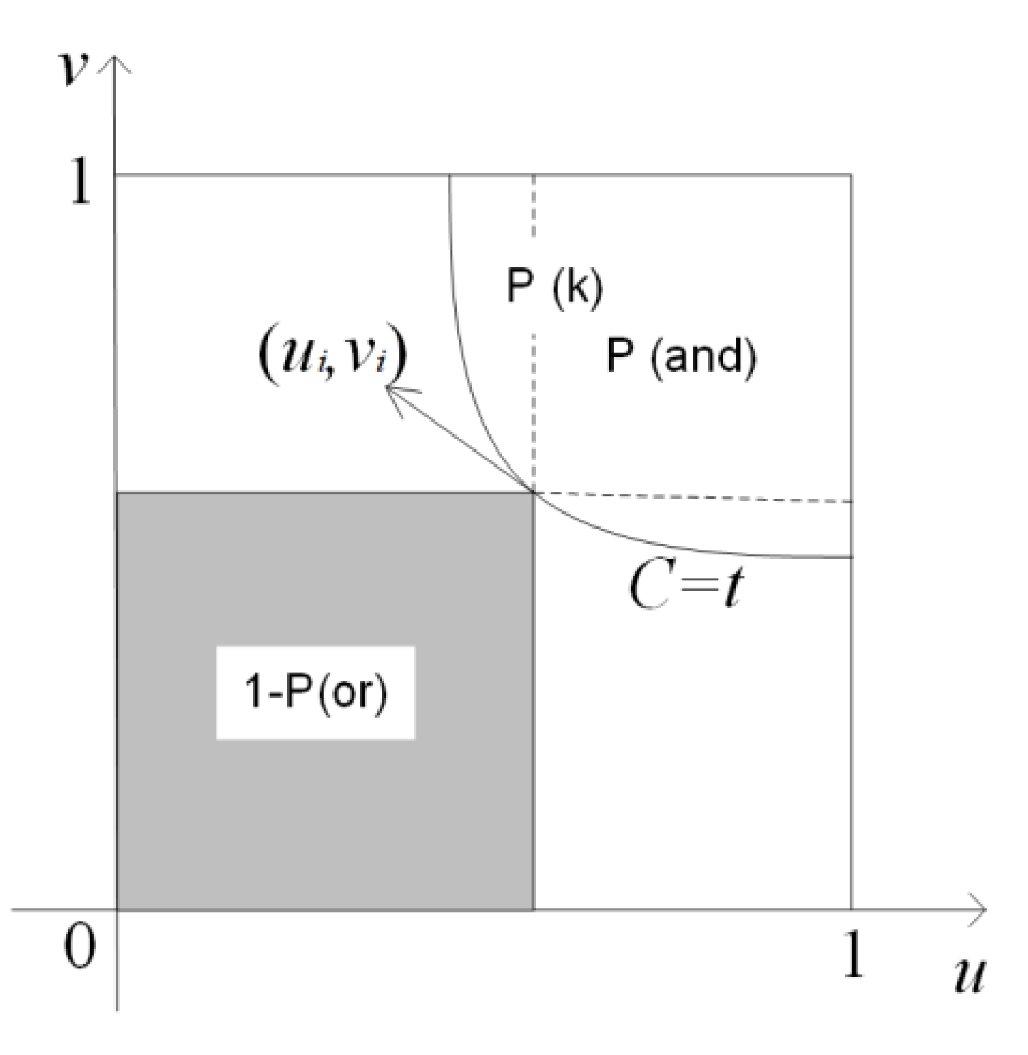
Three types of return periods have been proposed the two- and three-dimensional cases in hydrology, which are “AND”, “OR”, and Kendall return periods. Figure 2 illustrates the difference between the three return periods in a two-dimensional case.
In Figure 2, u and v represent the marginal distributions of two indicators X1 and X2 (F(X1) = u, F(X2) = v), respectively. C(ui, vi) = t is the joint probability for a given (ui, vi). The three return periods are defined based on three different types of probability expressions. The space formed by the dotted lines, u = 1 and v = 1 in the upper right corner indicates the probability that both the two indicators exceed their threshold values P{u> ui ∩ v> vi}. The return period corresponding to the simultaneous occurrence of two events can be expressed as
For a three-dimensional case, in which three indicators exceeding their thresholds simultaneously, the joint return period is shown as
where X1, X2, and X3 represent extreme indicators; x1, x2, and x3 are the certain thresholds of the indicators; F(x), F(x1,x2), …, F(x1,x2,x3) denote the cumulative probability distributions (CDFs) or joint CDFs corresponding to the thresholds; u, v, and w represent the marginal distributions of the indicators; and C(u,v), …, C(u,v,w) stand for copula functions describing joint distributions of extreme precipitation indicators.
The remaining space excluding the shadow part in Figure 2 indicates the probability that at least one of the two indicators exceeds the threshold (P{u > ui ∪ v > vi}). The corresponding return period expressed by can be calculated as
For the three-dimensional case, in which at least one of the three indicators exceeding the threshold, the return period can be expressed as
The space formed by the curve C = t, u = 1 and v = 1 (C = t is a surface in the three-dimensional case) represents the probability P(k) = P(C > t), and the corresponding Kendall return period is 1/P(k). The Kendall return period is calculated by introducing the Kendall measure Kc [38]:
For bivariate Archimedean copulas, Kc can be calculated from the generators of the copula functions. For the t copula, Gaussian copula and Archimedean copulas of three or higher dimensions, the Kc can hardly be calculated directly. In this study, the random sampling algorithm (10,000 sampling in this study) is used to estimate Kc [39], and then Kendall return periods of all two-dimensional and three-dimensional cases are obtained. Sampling algorithm steps to estimate Kc:
- Simulate a sample u1, ..., um from the d-dimensional copula C;
- For i = 1 ,..., m calculate wi = C(ui);
- Estimate Kc: .
4. Case Study and Results Analysis
4.1. Case Study
In order to quantitatively assess the changes in extreme precipitation from different perspectives, a number indicators focusing on various aspects of extreme precipitation have been proposed. According to the recommendations of the World Meteorological Organization, other relevant studies [14,15], four extreme precipitation indicators are used in this study to describe extreme precipitation features in Loess Plateau, including, the amount (P95), the number of days (D95), the intensity (I95), and the proportion (R95) of extreme precipitation. Detailed definitions of these indicators are shown in Table 1.
Six two-dimensional and three three-dimensional combination schemes of the four indicators can be formulated. The indicator combination schemes are shown in Table 2, and the joint return period of “AND”, “OR”, and Kendall for these combinations are characterized. Taking “AND” return periods of the combination events of {D95, P95} and {D95, P95, R95} as examples, the combination {D95, P95} indicates D95 and P95 simultaneously exceed their thresholds (Equation (10)), which means that an extreme precipitation event with long time and large amount would happen and severe flood may occur. The combination {D95, P95, R95} indicates that an extreme precipitation event with long duration and large amount occurs, and the proportion of this event to annual precipitation also exceeds the threshold (Equation (11)). For the reason that the annual rainfall is largely completed by extreme precipitation in this situation, adaptation strategies should be devised to achieve reasonable storage of water resources in the flood season and allocation of water resources throughout the year. The meaning of the other types of return periods for each joint event can be inferred from the definitions in Section 3.2.2.
The spatial risk characteristics for single indicators and multi-indicator combinations throughout the Loess Plateau can be obtained from the results over all stations in the region. In order to explore the trend in different extreme precipitation indicators and their joint risks, a 30-year moving window approach is applied. From the beginning of 1959–1988 to the end of 1989–2018, 31 groups of results for all stations were obtained. For each group, every indicator is fitted with marginal distribution (the GMM) and copulas are fitted for all two and three-dimensional combinations. The initial group (from 1959 to 1988) and the final group (from 1989 to 2018) of the 31 results belong to two independent time periods. The comparison of the results for these two groups can directly reflect the changes of extreme precipitation in the past two representative periods. By evaluating the outcomes of 31 groups in time series, the trend for both the univariate and multivariate risks can then be obtained. The Mann–Kendall (MK) test [40] is applied to evaluate whether the trend is significant, and the linear regression method is used to quantitative assess the degree of change. The annual extreme precipitation indicators are used in this study, and the Mann–Kendall test is basically not affected by serial correlation.
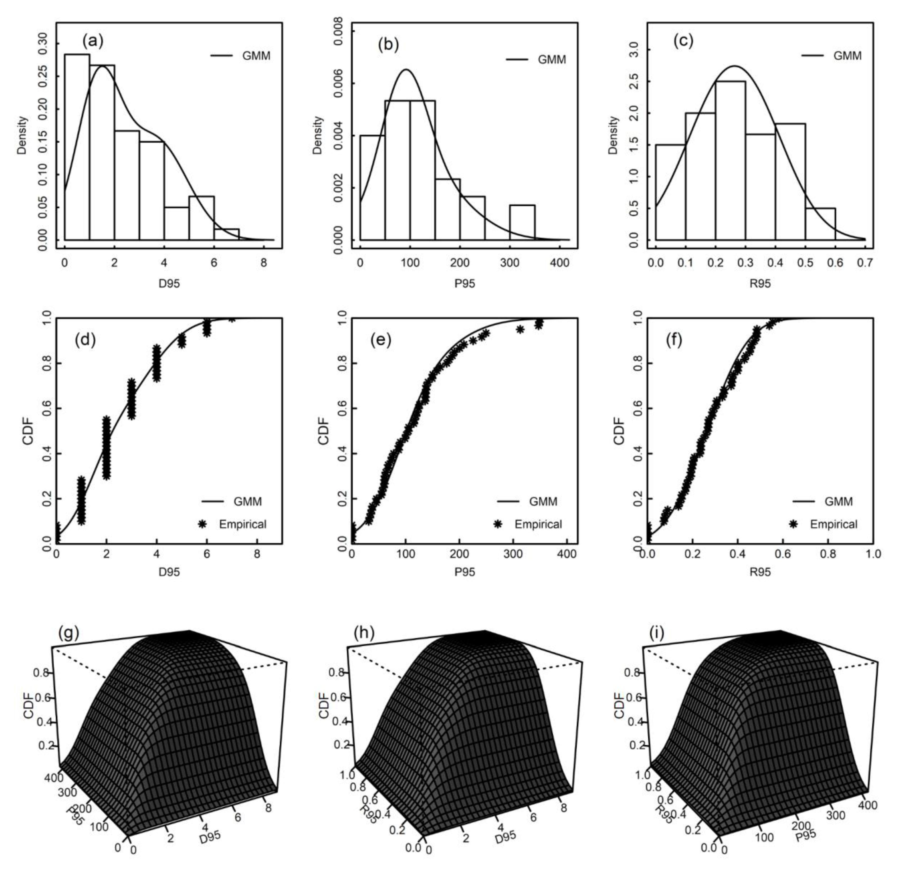
Taking Yulin station (Station 34 in Figure 1) as an example, the whole calculation process for the three indicators of P95, D95, and R95 during the period 1959–1988 is illustrated. GMM is used to construct the marginal distributions for the three indicators, and the test results of KS, RMSE, and AIC are shown in Table 3. Table S1 in the Supplementary Materials also shows the statistical test comparisons between GMM and the best fitted ones of five other commonly used parametric distributions (Gamma, Pearson type III (P III), lognormal (LN), Log Pearson type III (LP III), and generalized extreme value (GEV)) [23]. The p-values of KS tests are all greater and the AIC values are all smaller for GMM than other parametric distributions. Figure S1 shows the PDF fitting results of GMM with other parameter distributions in Table S1. It can be seen that even in the case of non-multimodal PDF, the performance of GMM can be similar to the optimal parameter distribution (Figure S1c) or even better (Figure S1b). Candidate copulas of Frank Gumbel, Gaussian, and t copulas (at two- or three-dimensional forms) are applied to build the joint probability distributions of multi-indicator combinations. The optimal copulas selected according to the KS, RMSE and AIC tests are shown in Table 3, and the corresponding test values are also displayed. It can be seen that the p-values of KS test for all indicators and multi-indicator combinations are all greater than 0.05, which means that the fitted distributions can effectively describe the probability characteristics of the indicators in various dimensions. The test results of the other copulas such as Frank and Gumbel are shown in Table S2 in the Supplementary Materials. Figure 3a–f further shows the goodness-of-fit by comparing the empirical PDFs and CDFs with those from GMM distributions of the three indicators, and the theoretical distributions show good agreements with the empirical distributions. Figure 3g–i shows the bivariate CDFs for three two-dimensional indicator combinations.
Given the 10-year univariate return period of three indicators, joint return periods of “AND”, “OR”, and Kendall for two- and three-dimensional cases are then evaluated. It can be seen from Table 4 that, for the same indicator combination scheme, the ranking order of the three return periods is Tor < Tk (Kendall return period) < Tand. This can also be inferred from the corresponding probabilities of various return periods in Figure 2, that is, P(and) < P(k) < P(or). Compared to the two-dimensional cases, it can be found that the Tor of the three-dimensional return period is smaller. The maximum return period (17.45 years) can be found when the three indicators occur simultaneously.
4.2. Changes of Different Schemes in Two 30-Year Stages
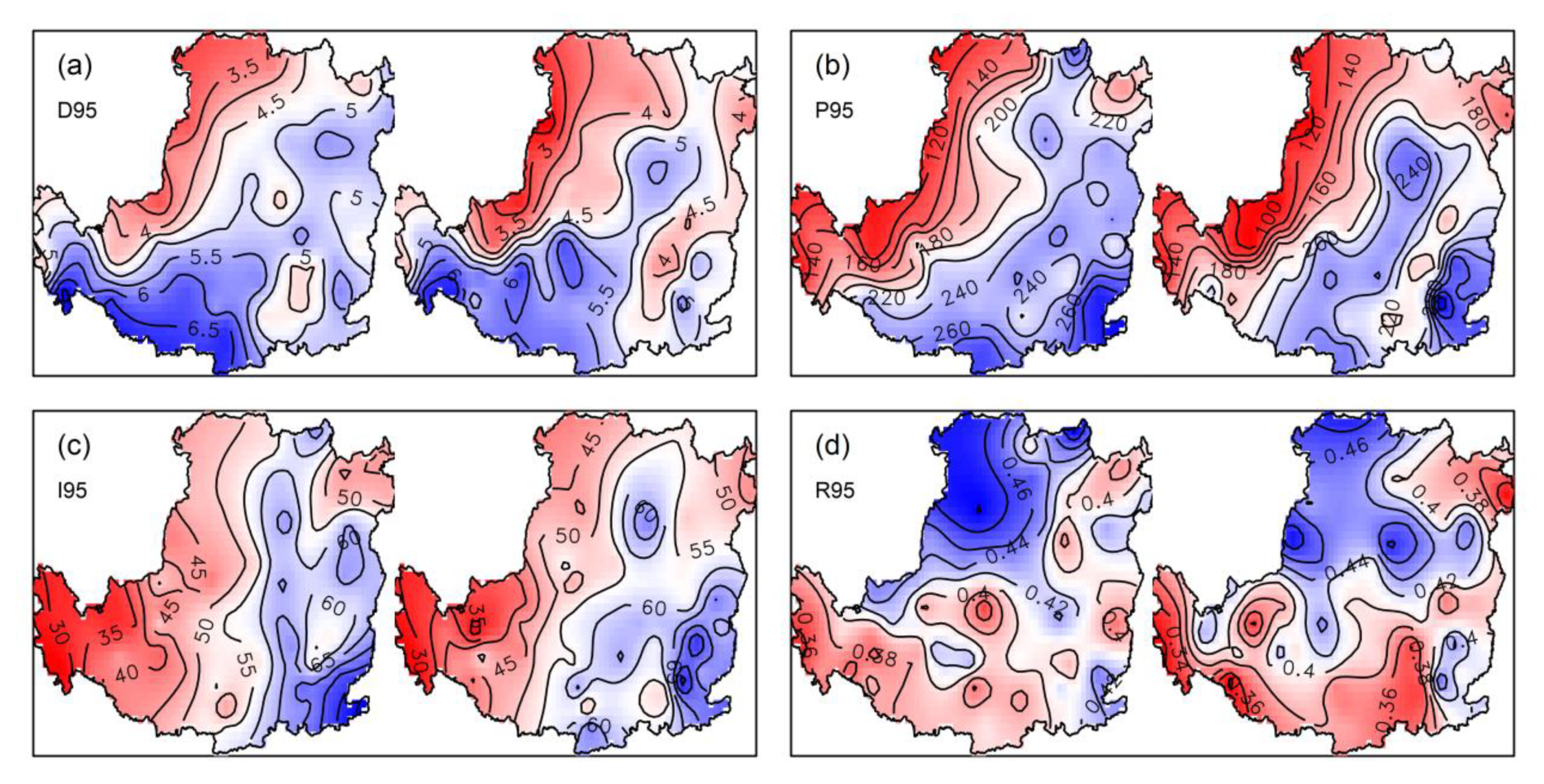
Based on the fitted GMM distributions, for a given return period, the values of the corresponding indicators can be obtained through the univariate return period formula (Equation (9)). In order to conduct a more illustrative comparison of the 10-year return period values between different regions, the values of four indicators at all stations under two 30-year periods are interpolated to the whole region by using the Kriging method (Figure 4). Figure 4a–d provides the comparisons of four indicator values between the time period of 1959–1988 (T1 period, left ones) and time period of 1989–2018 (T2 period, right ones).
The results show that the univariate return period values of the 10-year stage for all groups are similar in spatial distribution between the two 30-year stages over the entire region. The minimum values of D95 and P95 appear in the northwest of Loess Plateau, and there is a stepwise increasing trend from northwest to southeast for these two indicators. In the southeastern area, it is more prone to heavy rainfall for a long time (D95), which brings greater amounts of precipitation (P95). The values of I95 exhibit obvious increasing direction from west to east, while R95 presents a clear North–South gap. The mean values (averaged over the stations) of D95, P95, and I95 in Region 1 are 0.67 days, 78.2 mm, and 15.6 mm/day smaller than those in Region 2 for T1 period. Also, these indicators in Region 1 are 0.63 days, 81.2 mm, and 16.7 mm/day smaller than those in Region 2 for T2 period. The mean value of R95 in Region 1 is slightly higher than that in Region 2, and the values of R95 could be above 0.5 in the north part of Region 1. This indicates that, with the least annual precipitation in the northwest, nearly half of the annual precipitation would fall by extreme heavy precipitation.
The spatial distributions of the indicator values behave differently between the two time periods. The 10-year return period values of the four indicators in the T2 period (1989–2018), when compared with those in T1 period (1959–1988), exhibit the following changes. The value of D95 decreases slightly throughout the region, with an average decrease of 0.26 days. The station with the largest decrease of D95 appears in the northeast with a decrease of 1.95 days, whereas the station with the largest growth of D95 appears in the southwest region with an increase of 1.2 days. Similar to the changes of D95, P95 decreases significantly in north and southeast, with an average decrease of 13.13 mm. I95 increases significantly in some stations in the southwest and southeast regions with the largest increase of 9.96 and 25.4 mm/day, respectively. The spatial difference of R95 in different time periods is not obvious, and the change of annual precipitation does not bring obvious change of R95. Table 5 displays the average changes of four indicators in different regions and the number of stations which show growth changes by comparing with that in T1 period.
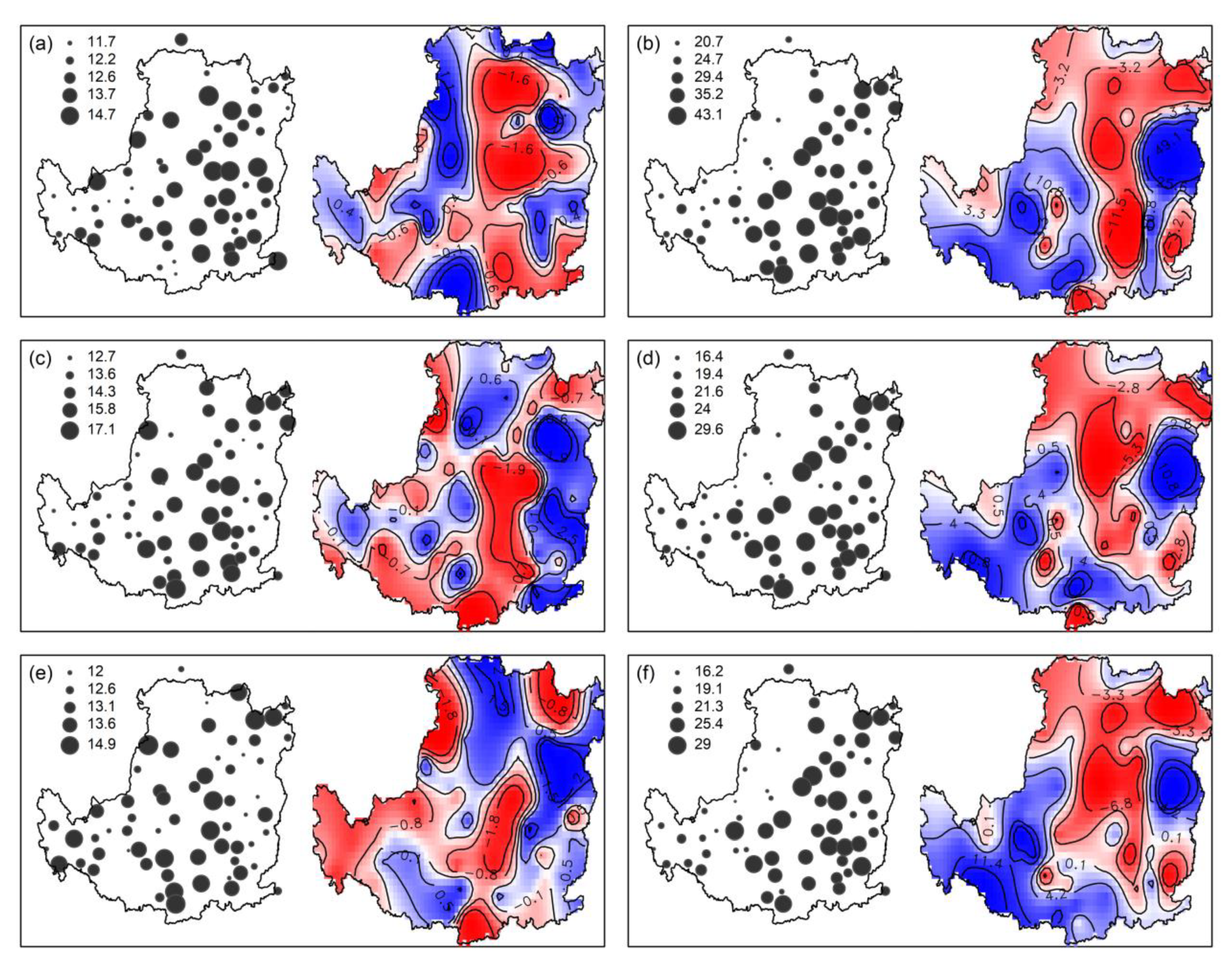
Under the condition that the indicator values at a 10-year return period, the joint return periods of Tand for two-dimensional or three-dimensional indicator combinations can then be obtained. Figure 5 shows Tand at each station in T1 period (i.e., 1959–1988) (sub-graphs on the left) of six two-dimensional indicator combinations, and the spatial changes in T2 (i.e., 1989–2018) compared with that in the T1 period (right ones of each group). The red areas in the right sub-graphs indicate decreasing Tand in past 30 years, which signify that the regions are more prone to joint risk than the T1 period.
The averaged Tand of three two-dimensional combination events {D95, P95}, {D95, R95}, and {P95, R95} in the T1 period are 13.05, 14.68, and 13.35 years, respectively. The Tand values are only slightly longer than the return period of a single event (10 years), and the minimum values of the three combined events are 11.03, 12.25, and 11.31 years, respectively. It is proved that these three groups of combination events are extremely easy to happen, and the events of different indicators in each combination at a 10-year return period level usually occur together. There is no obvious regularity in the spatial distributions of Tand for these three combinations. The spatial distributions of the changes in Tand for the three groups in T2 period by comparing with that in T1 are obviously different from each other. It is worth noticing that in the central region of the Loess Plateau, the return periods of the three indicator combinations are all decreased, indicating that increased chances for occurrence of the three joint events in this region.
The mean Tand values of the other three two-dimensional combination events of {D95, I95}, {P95, I95}, and {I95, R95} are 32.65, 22.37, and 22.45, respectively. The occurrence probability is relatively small compared with the above three combinations, but the severity of the events may be far greater than the former ones. For example, {D95, I95} represents a long-time heavy rainfall event with high precipitation intensity. For these three combination events, their spatial distributions of Tand are basically the same (T1 period), and their spatial distributions of changing trend in the past 30 years are also similar to each other. The three combination events share a common feature that all of them contain the I95 index. The above results may be because the joint distributions are significantly affected by the I95 indicator, which means that the contribution of I95 to the joint return period is far greater than other indicators. The Tand of the three combined events in the past 30 years have decreased greatly in the northern and central regions, which implies the occurrence probability of extreme joint events has increased significantly. A comprehensive evaluation of Tand of the six two-dimensional indicator combinations shows that the probability of all the six joint extreme events in the central part of the region has increased.
Figure 6 shows the Tand values of three three-dimensional indicator combinations at each station in 1959–1988, and also the spatial changes in 1989–2018 compared with that in the T1 stage. The Tand values of {D95, P95, R95} are significantly smaller than those for the other two groups, with an average of only 15.53 years in 1959–1988. For the two three-dimensional events that contain the precipitation intensity indicator, the Tand values are generally greater than that of the rest one. The mean Tand of {D95, I95, R95} and {P95, I95, R95} from 1959 to 1988 is 31.2 and 24.8 years, respectively. The spatial distribution and the change direction of joint return periods of the two events are similar with each other and are also similar to those for the two-dimensional events in Figure 5b,d,e. In T1 stage, the Tand values of {D95, I95, R95} and {P95, I95, R95} in Region 1 are generally smaller than those in Region 2. Figure 6b,c shows that the change direction of Tand in T2 stage compared with T1 stage has decreased in the northern and central regions, and increased in other regions. This may also be because the Tand values of different combination events are highly affected by the precipitation intensity indicator. In the north part of Region 1, where extreme precipitation occurs frequently in T1 stage, the three-dimensional Tand get even smaller in T2 stage.
Figures S2–S5 (in the Supplementary Materials) provide the Tk and Tor values of two- and three-dimensional indicator combinations at each station in 1959–1988, and the spatial changes in 1989–2018 compared with those in the T1 stage. In two-dimensional cases at T1 stage, the Tk values are all smaller than Tand over all stations (see explanation in Section 4.1) and are similar to Tand in magnitude distribution and change direction. The average Tk values corresponding to Figure S2a–f are 1.55, 10.09, 2.37, 5.66, 1.72, and 5.73 years smaller than those of Tand, respectively. The magnitude distribution of Tor values in T1 stage are opposite to Tand, as well as the change direction in T2 stage. This is because, given the CDF values of two indicators, the value of Tand is only related to bivariate CDF like Tor (Equations (10) and (12)). With the change of one bivariate CDF, the change directions of the two return periods are opposite with each other. In three-dimensional cases at T1 stage, the average TK values corresponding to Figure S3a–c are, respectively, 2.82, 8.80, and 6.83 years smaller than Tand. The average Tor values in Figure S5a–c are only 6.98, 5.50, and 5.82 years, respectively.
4.3. The Trend of Return Period of Multidimensional Moving Window Series
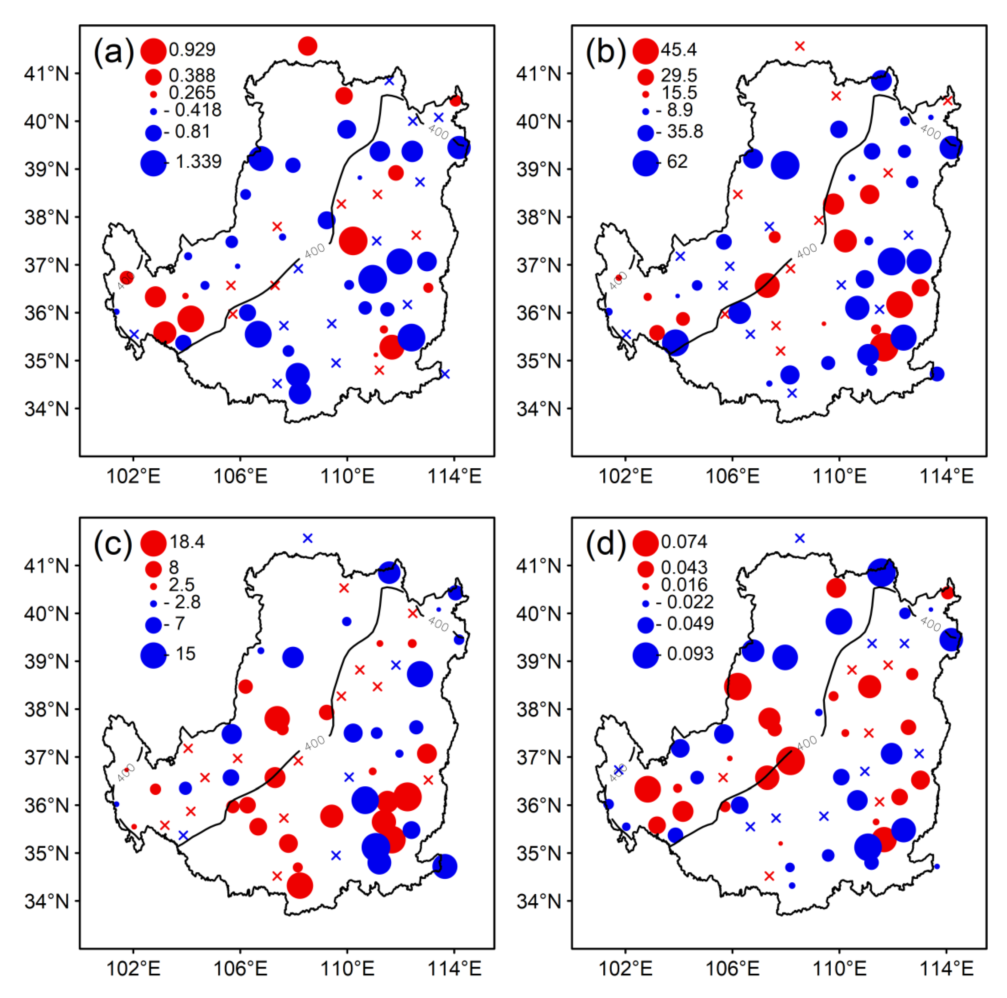
Figure 7 shows the changing trends in 10-year return period values for the four individual indicators calculated from the 30-year moving time series over all stations. The significance of changing trend and magnitude are also displayed in Figure 7. Table 6 provides statistics on the proportion of stations with significant increasing/decreasing trends, and average changes in the two regions. The results show that in the semi-arid area of the Loess Plateau (Region 1), the changing trends of D95 and P95 are similar in significance and direction. The 10-year return period values exhibit a significant decrease trend for D95 and P95 at 46% and 38% of the stations, respectively. However, some stations in the southwest area show a significant increasing trend. For these two indicators in Region 2, 42% and 50% of the stations display a significant decreasing trend, while only 16% and 24% of the stations show a significant increasing trend. Forty-two percent of the stations in Region 2 show a significant decreasing trend for I95, with a decrease ranging in magnitude from 2.2 to 31.6 mm/day. The southern region generally exhibits a significant increase in extreme precipitation intensity, which may increase the risk of flooding in that region. The distribution of stations with significant decreasing trends of R95 is consistent with that of P95. However, more stations in the southern part of Region 1 show significant increasing trends. The proportion of extreme precipitation in annual precipitation increases. This means that the precipitation concentration degree increases, which will aggravate the spatial–temporal distribution of precipitation
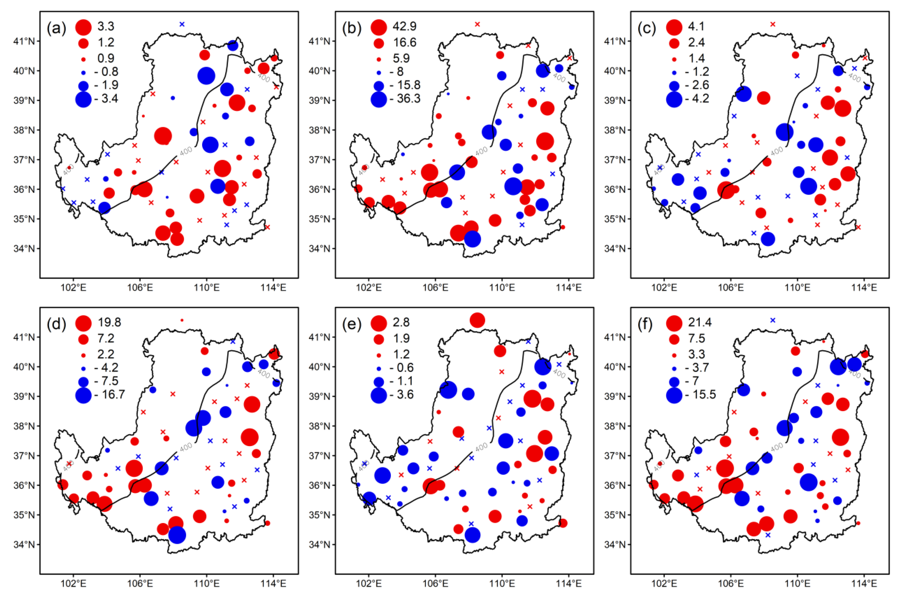
Figure 8 displays the significance and magnitude of the changing trends for Tand of the six two-dimensional indicator combinations based on the 30-year moving time series over all stations. Figure 8b,d,f shows that the joint return periods of three two-dimensional events {D95, I95}, {P95, I95}, and {I95, R95} in the whole region present a relatively consistent trend. The joint return periods of these three events in the entire region show significant increasing trends at 30, 25, and 29 stations, respectively. Moreover, 19 of them are shared stations, and these stations are mainly located in the south of Region 1. There are 17, 16, and 19 stations showing significant decreasing trends, 14 of which are shared stations, which are mainly located in the middle and north parts of the Loess Plateau. The average reductions in the Tand return period are 26.8, 9.25, and 9.39 years for the three events, respectively. These results suggest that the possibility of flood events with long time and high intensity in the middle of the Loess Plateau would increase. The decrease in Tand indicates that extreme precipitation events with the same degree occur more frequently. For the other three two-dimensional combined events, it can be seen that the return period of Tand for {P95, R95} is most significantly reduced in the entire region, with a total number of 24 stations showing a significant decreasing trend.
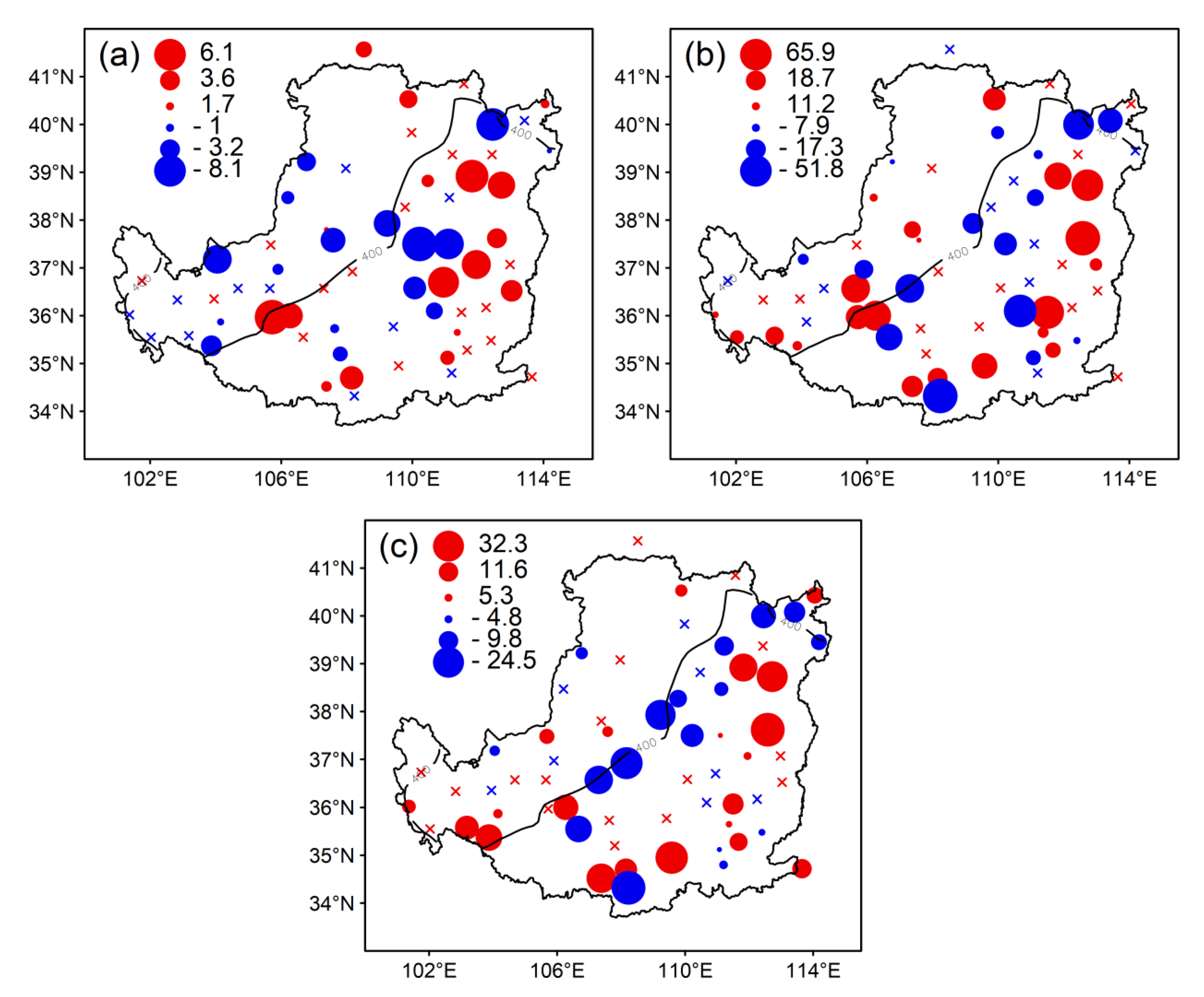
Figure 9 shows the significance and magnitude of the trends in joint return periods of Tand for three-dimensional indicator combinations over all stations. It can be seen that some stations in the central region of Loess Plateau exhibit significant downward trends for all three-dimensional events. The changing trend of Tand for {D95, P95, R95} in the middle of Region 2 shows a considerable differentiation state: The changing trend for stations in the western region decreased significantly, whereas those in the eastern region increased significantly. The stations with significant decreasing trend in Tand for {D95, P95, R95} are mainly located in the sub-humid regions, with an average reduction of 20.5 years. However, the stations with significantly decreasing return periods for {P95, I95, R95} are located near the boundary of 400 mm rainfall, with an average decrease of 13.5 years. This means that the combination event of {P95, I95, R95} in the semi-arid and semi-humid junction area tends to be more frequent.
Figures S6–S9 in the Supplementary Materials show the significance and magnitude of the trend changes for Tk and Tor for the two- and three-dimensional situations over all stations. In two-dimensional cases, the Tor and Tand basically show opposite changing trends, whereas Tk and Tand show similar changing trends and directions, with only differences in magnitude. For example, for {D95, I95}, {P95, I95} and {I95, R95}, the number of stations showing an increasing trend in Tk are 30, 23, and 25, respectively, in which 29, 22, and 24 stations are shared with the Tand cases. For the events of {D95, I95, R95} and {P95, I95, R95}, the stations with significant decreasing trends in Tk (mainly located in the central Loess Plateau) decreased by an average of 10.61 and 5.05 years, respectively. The sites with significant decrease trends in Tor are mainly located in the southwest and northeast parts of Loess Plateau.
5. Discussions and Conclusions
Compared with the previous studies, this study presents several outstanding features in multivariate risk inferences: (i) The joint risks of multidimensional indicators are evaluated in this study. (ii) Three types of joint return periods, including “AND”, “OR”, and Kendall, are evaluated for both two- and three-dimensional indicator combinations. (iii) By using the moving window approach, the proposed approach can quantitatively evaluate the spatial–temporal changes in risks of multidimensional cases. (iv) The GMM is used in fitting the marginal distributions for all indicators, which helps reduce the uncertainty brought by marginal model selection. The Kendall return period for high-dimensional copulas and two-dimensional elliptical copulas based on the random sampling algorithm is another innovation in this field.
The developed extreme precipitation assessment framework is applied in the Loess Plateau, China. The results indicate that the mean values of P95, D95, and I95 at 10-year return period in Region 1 (arid and semi-arid climate) are all smaller than those in Region 2 (semi-humid climate). However, the mean value of R95 in Region 1 is slightly higher than that in Region 2, and nearly half of the annual precipitation would occur by extreme heavy precipitation in the north of Region 1. Given the values of the indicators at 10-year return period, the combined events of {D95, P95}, {D95, R95}, {P95, R95}, and {D95, P95, R95} are extremely easy to occur in the Loess Plateau. The occurrence probability for combined events with the I95 indicator is relatively small compared with other combinations. The spatial distributions of changing trends in joint return periods for the multidimensional events containing the I95 indicator are generally the same. In the central region of Loess Plateau, the Tand values of all joint extremes are decreased. Tk values are smaller than Tand over all stations and are similar to Tand in magnitude distribution and change direction. The magnitude distribution of Tor values in T1 stage are opposite to Tand, as well as the change direction in T2 stage.
The provided assessment framework is repeatable and can be effectively transferred to other research areas to explore the spatial–temporal changes in multidimensional characteristics of extreme precipitation under climate change. Thanks to the development of climate models, this framework can also be used to project multidimensional probability variation characteristics of future extreme precipitation under different scenarios [41]. A variety of return period assessment methods are available to meet the needs of different hydrologic designs, and can help provide countermeasures for possible changes in floods and other secondary disasters.
Supplementary Materials
The following are available online at https://www.mdpi.com/2073-4441/12/4/1217/s1, Figure S1: Comparisons between GMM and other probability density estimates with theoretical frequency at Yulin Station: (a) PDF for D95, (b) PDF for P95, (c) PDF for R95, Figure S2: Joint return periods (Tk) at each station in 1959-1988 (left ones) and spatial changes in 1989-2018 (right ones) for six two-dimensional indicator combinations: (a) {D95, P95}, (b) {D95, I95}, (c) {D95, R95}, (d) {P95, I95}, (e) {P95, R95}, and (f) {I95, R95}, Figure S3: Joint return periods (Tk) at each station in 1959-1988 (left ones) and spatial changes in 1989-2018 (right ones) for three three-dimensional indicator combinations: (a) {D95, P95, R95}, (b) {D95, I95, R95}, and (c) {P95, I95, R95}, Figure S4: Joint return periods (Tor) at each station in 1959-1988 (left ones) and spatial changes in 1989-2018 (right ones) for six two-dimensional indicator combinations: (a) {D95, P95}, (b) {D95, I95}, (c) {D95, R95}, (d) {P95, I95}, (e) {P95, R95}, and (f) {I95, R95}, Figure S5: Joint return periods (Tor) at each station in 1959-1988 (left ones) and spatial changes in 1989-2018 (right ones) for three three-dimensional indicator combinations: (a) {D95, P95, R95}, (b) {D95, I95, R95}, and (c) {P95, I95, R95}, Figure S6: The significance and magnitude of the trends in joint return periods (Tk) over 30-year moving window series for six two-dimensional indicator combinations: (a) {D95, P95}, (b) {D95, I95}, (c) {D95, R95}, (d) {P95, I95}, (e) {P95, R95}, and (f) {I95, R95}, Figure S7: The significance and magnitude of the trends in joint return periods (Tk) over 30-year moving window series for three three-dimensional indicator combinations: (a) {D95, P95, R95}, (b) {D95, I95, R95}, and (c) {P95, I95, R95}, Figure S8: The significance and magnitude of the trends in joint return periods (Tor) over 30-year moving window series for six two-dimensional indicator combinations: (a) {D95, P95}, (b) {D95, I95}, (c) {D95, R95}, (d) {P95, I95}, (e) {P95, R95}, and (f) {I95, R95}, Figure S9: The significance and magnitude of the trends in joint return periods (Tor) over 30-year moving window series for three three-dimensional indicator combinations: (a) {D95, P95, R95}, (b) {D95, I95, R95}, and (c) {P95, I95, R95}., Table S1: Statistical test comparisons between GMM and the best fitted ones of five other distributions (Gamma, Pearson type III (P III), lognormal (LN), Log Pearson type III (LP III), generalized extreme value (GEV)) at Yulin Station, Table S2: Statistical test results for copulas at Yulin Station.
Author Contributions
Conceptualization, C.S.; methodology, C.S. and Y.F.; software, C.S.; validation, Y.F., and C.S.; formal analysis, C.S.; investigation, C.S.; resources, G.H.; data curation, C.S.; writing—original draft preparation, C.S.; writing—review and editing, Y.F. and G.H.; visualization, C.S.; supervision, G.H.; project administration, G.H.; funding acquisition, G.H. All authors have read and agreed to the published version of the manuscript
Funding
This research was supported by the National Key Research and Development Plan (2016YFA0601502), the Natural Sciences Foundation (51520105013, 51679087), the 111 Program (B14008), the Natural Science and Engineering Research Council of Canada, and the Fundamental Research Funds for the Central Universities (2016XS89).
Conflicts of Interest
The authors declare no conflict of interest.
References
- Aguilar, E. Changes in temperature and precipitation extremes in western Central Africa, Guinea Conakry, and Zimbabwe, 1955–2006. J. Geophys. Res. 2008, 114, D02115. [Google Scholar] [CrossRef]
- Ullah, S.; You, Q.; Ullah, W.; Ali, A. Observed changes in precipitation in china-pakistan economic corridor during 1980–2016. Atmos. Res. 2018, 210, 1–14. [Google Scholar] [CrossRef]
- Lu, W.; Qin, X.S.; Jun, C. A parsimonious framework of evaluating WSUD features in urban flood mitigation. J. Environ. Inform. 2019, 33, 17–27. [Google Scholar] [CrossRef]
- IPCC. Climate Change 2007: The Physical Science Basis. Contribution of Working Group I to the Fourth Assessment Report of the Intergovernmental Panel on Climate Change; Cambridge University Press: Cambridge, UK, 2007. [Google Scholar]
- Shivam, G.; Goyal, M.K.; Sarma, A.K. Index-based study of future precipitation changes over subansiri river catchment under changing climate. J. Environ. Inform. 2019, 34, 1–14. [Google Scholar] [CrossRef]
- Rudari, R.; Entekhabi, D.; Roth, G. Terrain and multiple-scale interactions as factors in generating extreme precipitation events. J. Hydrometeorol. 2004, 5, 390–404. [Google Scholar] [CrossRef]
- Merino, A.; Fernández-González, S.; García-Ortega, E.; Sánchez, J.L.; López, E.; Gascón, L. Temporal continuity of extreme precipitation events using sub-daily precipitation: Application to floods in the ebro basin, northeastern Spain. Int. J. Climatol. 2018, 38, 1877–1892. [Google Scholar] [CrossRef]
- Shaffie, S.; Mozaffari, G.A.; Khosravi, Y. Determination of extreme precipitation threshold and analysis of its effective patterns (case study: West of Iran). Nat. Hazards 2019, 99, 857–878. [Google Scholar] [CrossRef]
- Šraj, M.; Viglione, A.; Parajka, J.; Blöschl, G. The influence of non-stationarity in extreme hydrological events on flood frequency estimation. J. Hydrol. Hydromech. 2016, 64, 426–437. [Google Scholar] [CrossRef] [Green Version]
- Mondal, A.; Daniel, D. Return levels under nonstationarity: The need to update infrastructure design strategies. J. Hydrol. Eng. 2019, 24, 04018060. [Google Scholar] [CrossRef]
- Li, H.; Wang, D.; Singh, V.P.; Wang, Y.; Wu, J.; Wu, J.H.; Liu, J.; Zou, Y.; He, R.; Zhang, J. Non-stationary frequency analysis of annual extreme rainfall volume and intensity using Archimedean Copulas: A case study in eastern China. J. Hydrol. 2019, 571, 114–131. [Google Scholar] [CrossRef]
- Lloyd, E.A.; Oreskes, N. Climate change attribution: When is it appropriate to accept new methods? Earth’s Future 2018, 6, 311–325. [Google Scholar] [CrossRef]
- Vasquez, R.; Diego, J. Evaluating Hydrologic Design under Stationary and Non-Stationary Assumptions. Ph.D. Thesis, University of California, Irvine, CA, USA, 2016. [Google Scholar]
- Ramos, M.C.; Martínez-Casasnovas, J.A. Trends in precipitation concentration and extremes in the mediterranean Penedes-Anoia region NE Spain. Clim. Chang. 2006, 74, 457–474. [Google Scholar] [CrossRef]
- Goswami, U.P.; Hazra, B.; Kumar, G.M. Copula-based probabilistic characterization of precipitation extremes over north sikkim himalaya. Atmos. Res. 2018, 212, 273–284. [Google Scholar] [CrossRef]
- Vincent, L.A.; Mekis, É. Changes in daily and extreme temperature and precipitation indices for Canada over the twentieth century. Atmos. -Ocean 2006, 44, 177–193. [Google Scholar] [CrossRef] [Green Version]
- Gao, Y.; Feng, Q.; Liu, W.; Lu, A.; Wang, Y.; Yang, J.; Cheng, A.; Wang, Y.; Su, Y.; Liu, L.; et al. Changes of daily climate extremes in Loess Plateau during 1960–2013. Quat. Int. 2014, 371, 5–21. [Google Scholar]
- El Adlouni, S.; Ouarda, T.; Zhang, X.; Roy, R.; Bobee, B. Generalized maximum likelihood estimators for the nonstationary generalized extreme value model. Water Resour. Res. 2007, 43, W03410. [Google Scholar] [CrossRef]
- Dars, G.H. Climate Change Impacts on Precipitation Extremes over the Columbia River Basin Based on Downscaled CMIP5 Climate Scenarios. Master’s Thesis, Department of Civil & Environmental Engineering, Portland State University, Portland, OR, USA, 2013. [Google Scholar]
- Wehner, M. Sources of uncertainty in the extreme value statistics of climate data. Extremes 2010, 13, 205–217. [Google Scholar] [CrossRef] [Green Version]
- Ghosh, S.; Das, D.; Kao, S.C.; Ganguly, A.R. Lack of uniform trends but increasing spatial variability in observed indian rainfall extremes. Nat. Clim. Chang. 2011, 2, 86–91. [Google Scholar] [CrossRef]
- Fan, Y.R.; Huang, W.W.; Huang, G.H.; Li, Y.P.; Huang, K.; Li, Z. Hydrologic risk analysis in the yangtze river basin through coupling gaussian mixtures into copulas. Adv. Water Resour. 2016, 88, 170–185. [Google Scholar] [CrossRef] [Green Version]
- Sun, C.X.; Huang, G.H.; Fan, Y.; Zhou, X.; Lu, C.; Wang, X.Q. Drought occurring with hot extremes: Changes under future climate change on Loess Plateau, China. Earth’s Future 2019, 7, 587–604. [Google Scholar] [CrossRef] [Green Version]
- Salvadori, G.; De Michele, C. Frequency analysis via copulas: Theoretical aspects and applications to hydrological events. Water Resour. Res. 2004, 40. [Google Scholar] [CrossRef]
- Jhong, B.C.; Tung, C.P. Evaluating future joint probability of precipitation extremes with a copula-based assessing approach in climate change. Water Resour. Manag. 2018, 32, 4253–4274. [Google Scholar] [CrossRef]
- Liu, M.; Xu, X.; Sun, A.Y.; Wang, K.; Liu, W.; Zhang, X. Is southwestern china experiencing more frequent precipitation extremes? Environ. Res. Lett. 2014, 9, 064002. [Google Scholar] [CrossRef] [Green Version]
- Akaike, H. A new look at the statistical model identification. IEEE Trans. Autom. Control 1974, 19, 716–723. [Google Scholar] [CrossRef]
- Kurowicka, D.; Joe, H. Dependence Modeling: Vine Copula Handbook; World Scientific: Singapore, 2011; Available online: https://econpapers.repec.org/bookchap/wsiwsbook/7699.htm (accessed on 12 January 2020).
- Xu, K.; Yang, D.; Xu, X.; Lei, H. Copula based drought frequency analysis considering the spatio-temporal variability in southwest china. J. Hydrol. 2015, 527, 630–640. [Google Scholar] [CrossRef]
- Zhu, U.; Liu, Y.; Wang, W.; Singh, V.P.; Ma, X.; Yu, Z. Three dimensional characterization of meteorological and hydrological droughts and their probabilistic links. J. Hydrol. 2019, 578, 124016. [Google Scholar] [CrossRef]
- Wang, W.; Shao, Q.; Peng, S.; Zhang, Z.; Xing, W.; An, G.; Yong, B. Spatial and temporal characteristics of changes in precipitation during 1957–2007 in the Haihe river basin, China. Stoch. Environ. Res. Risk Assess. 2011, 25, 881–895. [Google Scholar] [CrossRef]
- Sondergaard, T.; Lermusiaux, P.F.J. Data assimilation with gaussian mixture models using the dynamically orthogonal field equations. part ii: Applications. Mon. Weather Rev. 2013, 141, 1761–1785. [Google Scholar] [CrossRef] [Green Version]
- He, J. Mixture model based multivariate statistical analysis of multiply censored environmental data. Adv. Water Resour. 2013, 59, 15–24. [Google Scholar] [CrossRef]
- Sklar, K. Fonctions dé repartition á n dimensions et leurs marges. Publ. Inst. Stat. Univ. Paris 1959, 8, 229–231. [Google Scholar]
- Nelsen, R.B. An Introduction to Copulas; Springer: New York, NY, USA, 2006. [Google Scholar]
- Sraj, M.; Bezak, N.; Brilly, M. Bivariate flood frequency analysis using the copula function: A case study of the Litija station on the Sava River. Hydrol. Process. 2015, 29, 225–238. [Google Scholar] [CrossRef]
- Zhang, L. Multivariate Hydrological Frequency Analysis and Risk Mapping. Ph.D. Thesis, Department of Civil and Environmental Engineering, Lousiana State University and Agricultural and Mechanical College, Baton Rouge, LA, USA, 2005. [Google Scholar]
- Genest, C.; Rivest, L.P. Statistical inference procedures for bivariate Archimedean copulas. J. Am. Stat. Assoc. 1993, 88, 1034–1043. [Google Scholar] [CrossRef]
- Salvadori, G.; De, M.C.; Durante, F. On the return period and design in a multivariate framework. Hydrol. Earth Syst. Sci. 2011, 15, 3293–3305. [Google Scholar] [CrossRef] [Green Version]
- Kendall, M.G. Rank Correlation Methods; Charles Griffin & Company Ltd.: London, UK, 1975. [Google Scholar]
- Wu, H.; Chen, B.; Snelgrove, K.; Lye, L.M. Quantification of Uncertainty Propagation Effects during Statistical Downscaling of Precipitation and Temperature to Hydrological Modeling. J. Environ. Inform. 2019, 34, 139–148. [Google Scholar] [CrossRef]
Figure 1.
Location of the Loess Plateau with 63 stations: (a) location of the Loess Plateau, (b) stations.
Figure 1.
Location of the Loess Plateau with 63 stations: (a) location of the Loess Plateau, (b) stations.

Figure 2.
Different types of return periods in two-dimensional case.

Figure 3.
The probability density functions (PDFs) and cumulative probability distributions (CDFs) for three precipitation indicators and bivariate CDFs for three indicator combinations at Yulin Station: (a) PDF for D95, (b) PDF for P95, (c) PDF for R95, (d) CDF for D95, (e) CDF for P95, (f) CDF for R95, (g) bivariate CDF for {P95, D95}, (h) bivariate CDF for {D95, R95}, and (i) bivariate CDF for {P95, R95}.

Figure 4.
The values of four extreme precipitation indicators at 10-year return period for time periods of 1959–1988 (left ones) and 1989–2018 (right ones): (a) D95, (b) P95, (c) I95, and (d) R95.
Figure 4.
The values of four extreme precipitation indicators at 10-year return period for time periods of 1959–1988 (left ones) and 1989–2018 (right ones): (a) D95, (b) P95, (c) I95, and (d) R95.

Figure 5.
Joint return periods (Tand) at each station in 1959–1988 (left ones) and spatial changes in 1989–2018 (right ones) for six two-dimensional indicator combinations: (a) {D95, P95}, (b) {D95, I95}, (c) {D95, R95}, (d) {P95, I95}, (e) {P95, R95}, and (f) {I95, R95}.
Figure 5.
Joint return periods (Tand) at each station in 1959–1988 (left ones) and spatial changes in 1989–2018 (right ones) for six two-dimensional indicator combinations: (a) {D95, P95}, (b) {D95, I95}, (c) {D95, R95}, (d) {P95, I95}, (e) {P95, R95}, and (f) {I95, R95}.

Figure 6.
Joint return periods (Tand) at each station in 1959–1988 (left ones) and spatial changes in 1989–2018 (right ones) for three three-dimensional indicator combinations: (a) {D95, P95, R95}, (b) {D95, I95, R95}, and (c) {P95, I95, R95}.
Figure 6.
Joint return periods (Tand) at each station in 1959–1988 (left ones) and spatial changes in 1989–2018 (right ones) for three three-dimensional indicator combinations: (a) {D95, P95, R95}, (b) {D95, I95, R95}, and (c) {P95, I95, R95}.

Figure 7.
Changing trends in 10-year return period values over 30-year moving window series for four indicators: (a) D95, (b) P95, (c) I95, and (d) R95. Blue dots indicate significant decreasing trends, red dots denote significant increasing trends, and the crosses indicate non-significant trend.
Figure 7.
Changing trends in 10-year return period values over 30-year moving window series for four indicators: (a) D95, (b) P95, (c) I95, and (d) R95. Blue dots indicate significant decreasing trends, red dots denote significant increasing trends, and the crosses indicate non-significant trend.

Figure 8.
The significance and magnitude of the trends in joint return periods (Tand) over 30-year moving window series for six two-dimensional indicator combinations: (a) {D95, P95}, (b) {D95, I95}, (c) {D95, R95}, (d) {P95, I95}, (e) {P95, R95}, and (f) {I95, R95}.
Figure 8.
The significance and magnitude of the trends in joint return periods (Tand) over 30-year moving window series for six two-dimensional indicator combinations: (a) {D95, P95}, (b) {D95, I95}, (c) {D95, R95}, (d) {P95, I95}, (e) {P95, R95}, and (f) {I95, R95}.

Figure 9.
The significance and magnitude of the trends in joint return periods (Tand) over 30-year moving window series for three three-dimensional indicator combinations: (a) {D95, P95, R95}, (b) {D95, I95, R95}, and (c) {P95, I95, R95}.
Figure 9.
The significance and magnitude of the trends in joint return periods (Tand) over 30-year moving window series for three three-dimensional indicator combinations: (a) {D95, P95, R95}, (b) {D95, I95, R95}, and (c) {P95, I95, R95}.


Table 1.
Concept of four extreme precipitation indicators.
| Indices | Abbreviations | Definitions | Unit |
|---|---|---|---|
| Number of extreme precipitation days | D95 | Number of days with P > 95th percentile (daily precipitation exceeding the 95th percentile of precipitation series during 1971–2000). | days |
| The amount of extreme heavy precipitation | P95 | Annual total amount of precipitation with P > 95th percentile | mm |
| The intensity of extreme precipitation | I95 | Average daily precipitation intensity of extreme precipitation | mm/day |
| Ratio of extreme precipitation | R95 | Ratio of annual total precipitation due to events exceeding the 95th percentile | - |
Table 2.
The two-dimensional and three-dimensional indicator combination schemes.
| ID | Combinations | ID | Combinations | ID | Combinations |
|---|---|---|---|---|---|
| 1 | {D95, P95} | 4 | {P95, I95} | 7 | {D95, P95, R95} |
| 2 | {D95, I95} | 5 | {P95, R95} | 8 | {D95, I95, R95} |
| 3 | {D95, R95} | 6 | {I95, R95} | 9 | {P95, I95, R95} |
Table 3.
Statistical test results for Gaussian mixture model (GMM) and best-fitted copulas at Yulin Station.
Table 3.
Statistical test results for Gaussian mixture model (GMM) and best-fitted copulas at Yulin Station.
| Scheme | Distribution | KS Test | RMSE | AIC | |
|---|---|---|---|---|---|
| p-Value | |||||
| D95 | GMM | 0.143 | 0.568 | 0.055 | −170.089 |
| P95 | GMM | 0.089 | 0.972 | 0.029 | −208.096 |
| R95 | GMM | 0.082 | 0.987 | 0.032 | −202.164 |
| {D95, P95} | Gaussian | 0.022 | 0.615 | 0.027 | −215.108 |
| {D95, R95} | t | 0.024 | 0.697 | 0.032 | −203.671 |
| {P95, R95} | Gaussian | 0.028 | 0.790 | 0.030 | −208.887 |
| {D95, P95, R95} | t | 0.032 | 0.648 | 0.021 | −228.451 |
KS test: the Kolomogorov-Smirnov test; : the value of the test statistic; p-Value: the significance level; RMSE: root mean square error; AIC: Akaike’s information criteria.
Table 4.
Joint returned periods of “AND” (Tand), “OR” (Tor), and Kendall (Tk) for two and three-dimensional cases.
Table 4.
Joint returned periods of “AND” (Tand), “OR” (Tor), and Kendall (Tk) for two and three-dimensional cases.
| Return Periods | {D95, P95} | {D95, R95} | {P95, R95} | {D95, P95, R95} |
|---|---|---|---|---|
| Tor | 8.09 | 7.28 | 7.79 | 7.01 |
| Tk | 11.66 | 13.50 | 11.77 | 12.66 |
| Tand | 13.09 | 15.99 | 13.96 | 17.45 |
Table 5.
Statistics of changes in four indicators in different regions.
| Region | Number of Stations | D95 | P95 | I95 | R95 | ||||
|---|---|---|---|---|---|---|---|---|---|
| A | N | A | N | A | N | A | N | ||
| 1 | 25 | −0.24 | 7 | −11.29 | 11 | 0.36 | 14 | −0.013 | 11 |
| 2 | 38 | −0.27 | 14 | −8.27 | 14 | 1.44 | 24 | −0.004 | 16 |
A: The average change over all stations in the region; N: Number of stations with increased value.
Table 6.
Statistical information on the increase and decrease trend of the four indicators in two regions: The proportion of stations with significant increasing trend (PI) and the total growth over the moving window series (TG); the proportion of stations with significant decreasing trend (PD) and total reduction over the moving window series (TD).
| Indices | Region 1 | Region 2 | ||
|---|---|---|---|---|
| PI/TG | PD/TD | PI/TG | PD/TD | |
| D95 | 0.31/0.54 | 0.46/−0.63 | 0.16/0.53 | 0.42/−0.95 |
| P95 | 0.19/22.04 | 0.38/−35.7 | 0.24/39.40 | 0.50/−37.01 |
| I95 | 0.27/6.79 | 0.38/−6.80 | 0.42/12.17 | 0.29/−11.63 |
| R95 | 0.38/0.05 | 0.46/−0.06 | 0.34/0.04 | 0.34/−0.05 |
© 2020 by the authors. Licensee MDPI, Basel, Switzerland. This article is an open access article distributed under the terms and conditions of the Creative Commons Attribution (CC BY) license (http://creativecommons.org/licenses/by/4.0/).
Share and Cite
MDPI and ACS Style
Sun, C.; Huang, G.; Fan, Y. Temporal and Spatial Characteristics of Multidimensional Extreme Precipitation Indicators: A Case Study in the Loess Plateau, China. Water 2020, 12, 1217. https://doi.org/10.3390/w12041217
AMA Style
Sun C, Huang G, Fan Y. Temporal and Spatial Characteristics of Multidimensional Extreme Precipitation Indicators: A Case Study in the Loess Plateau, China. Water. 2020; 12(4):1217. https://doi.org/10.3390/w12041217
Chicago/Turabian StyleSun, Chaoxing, Guohe Huang, and Yurui Fan. 2020. "Temporal and Spatial Characteristics of Multidimensional Extreme Precipitation Indicators: A Case Study in the Loess Plateau, China" Water 12, no. 4: 1217. https://doi.org/10.3390/w12041217
Note that from the first issue of 2016, this journal uses article numbers instead of page numbers. See further details here.