Fluid Structure Interaction of 2D Objects through a Coupled KBC-Free Surface Model


Department of Mechanical Engineering, University of Rome Niccolò Cusano, 00166 Rome, Italy
Water 2020, 12(4), 1212; https://doi.org/10.3390/w12041212
Submission received: 16 March 2020
/
Revised: 6 April 2020
/
Accepted: 21 April 2020
/
Published: 24 April 2020
(This article belongs to the Special Issue Combined Numerical and Experimental Methodology for Fluid–Structure Interactions in Free Surface Flows)
Abstract
:In this study, the capabilities of a coupled KBC-free surface model to deal with fluid solid interactions with the slamming of rigid obstacles in a calm water tank were analyzed. The results were firstly validated with experimental and numerical data available in literature and, thereafter, some additional analyses was carried out to understand the main parameters’ influence on slamming coefficient. The effect of grid resolution and Reynolds number were firstly considered to choose the proper grid and to present the weak impact of such a non-dimensional number on process evolution. Hence, the influence of Froude number on fluid-dynamics quantities was pointed out considering vertical impacts of both cylindrical, as in the references, and ellipsoidal obstacles. Different formulations of slamming coefficient were used and compared. Results are pretty encouraging and they confirm the effectiveness of lattice Boltzmann model to deal with such a problem. This leaves the door open to additional improvements addressed to the study of free buoyant bodies immersed in a fluid domain.
1. Introduction
Recently, always increasing attention has been addressed to the analysis of fluid structure interaction (FSI) between solid and fluid in relative motion. Such a problem is ubiquitous and present in a large number of engineering applications, which span from naval [1,2,3], to energy harvesting [4] and from to bio-engineering [4] to micro-mechanical problems [5]. To this aim, many models have already been developed both in traditional Navier–Stokes framework [6,7,8,9,10] and in alternative environments such as SPH [11,12] or lattice Boltzmann [13,14]. All these numerical models have been constantly compared and validated with the large number of experimental data available in literature, which, again, cover a wide range of applications [4,15,16,17,18].
It is worth highlighting how, in the recent past, due to the increased computational power availability, many efforts have been devoted in defining models for the contemporary solution of both fluid and solid motion/deformation [19]. In naval application, this reflects always increasing attention to the analysis of impulsive loads due to slamming of rigid/deformable wedges/obstacles [20,21]. With respect to lattice Boltzmann method (LBM), many studies have already been carried out considering both rigid and flexible obstacles interacting with fluid flows [22]. The majority of them treat a single phase fluid (i.e., air) without considering multiphase flows interactions, which may play a relevant role in phenomenon evolution. Recently, some authors have deeply analyzed the FSI problems dealt with LBM: De Rosis et al. studied both rigid and flexible obstacles in different engineering applications with particular focus on lamina-shaped obstacles and on coupling of different solvers [23,24,25]; Zarghami et al. studied the water entry problems of rigid obstacle with coupling standard Bhatnagar–Gross–Krook (BGK) operator and free-surface model [26]; and Dorschner et al. deeply investigated the entropic framework with advanced treatment of moving and deformable boundaries [27,28,29].
In this paper, the LBM with Karlin–Bösch–Chikatamarla (KBC) implementation [28,30] is coupled with a free-surface approach for dealing with multiphase interactions [31], including obstacle motion managed through Grad’s approximation [27]. Constant obstacle velocity was imposed during the simulation and the hydrodynamic force exchanged between fluid and obstacle was constantly evaluated during evolution. The coupled algorithm was first validated with some experimental and numerical findings [32,33], thus carefully compared with traditional BGK collision operator coupled with Smagorinsky sub-grid turbulence model [34,35]. The influence of both Reynolds and Froude non-dimensional numbers was analyzed considering the time evolution of slamming coefficient. The KBC framework was also used for the analysis of vertical impacts of differently shaped obstacles.
The paper is organized as follows. In Section 2, the numerical algorithm is presented with referring to all the implemented sub-systems, namely the LBM with BGK in Section 2.1, the KBC model in Section 2.2, the force evaluation and obstacle motion in Section 2.3, and the free-surface algorithm in Section 2.4. In Section 3, the developed model is validated with respect to both experimental and numerical data. In Section 4, the results for different object geometries are presented and commented. In Section 5, some conclusions and future work are summarized.
2. Numerical Model
In this section, a short overview of the numerical model adopted is briefly presented, starting from a general description of LB model to the boundary condition for moving obstacles.
2.1. Lattice Boltzmann Method
During the last decades, the lattice Boltzmann method has gained an important role in the computational fluid dynamics panorama, thanks to its simplicity in implementation [36,37,38] and the possibility to deal with a large range of applications (non-Newtonian [39], fluid–structure interaction [40,41], turbulent flows [29], etc.). The governing Boltzmann equation in discrete space of velocities reads as follows:
where represents the position of the particle, t is time, are the particle distribution functions, are the discrete speeds representative of directions along which particles can move, and is the relaxation time used to discretize the collision operator as described below in the text. It is clarified below how the left-had side (LHS) of Equation (1) represents the streaming step, while the right-hand side (RHS) the collision one. The former can be linearly solved in both time and space, while the latter needs some special treatment to be linearized. By explicitly solving the time derivative present in Equation (1), one can obtain:
which represents the commonly named discrete Boltzmann Equation (DBE), in the finite time . More specifically, the left-hand side of Equation (2) represents the streaming step, while the right-hand side is the collision operator, linearized as per the (BGK) approximation [42]. In many applications, this equation is solved within a uniform structured Cartesian grid. In the available literature, there are many studies focused on finding the optimal number of discrete velocities where the particles can move along to maintain the isotropy [43]. The simulations carried out in this study used a two-dimensional stencil with nine allowed particle directions, namely the , where D is the number of dimensions and Q is the number of allowed moving directions. With respect to the collision operator presented in Equation (2), the nonlinear terms are embedded in the equilibrium distribution functions , defined as follows:
where is the lattice speed of sound, is a set of weights normalized to unity, and and are the macroscopic fluid density and velocity. To retrieve macroscopic quantities from particles distributions, the first two moments of distribution functions are considered:
where refers to the number of distribution functions Q. For weakly compressible flows, in the limit of small Knudsen numbers, Equation (2) recovers the Navier–Stokes equations with pressure given by and kinematic viscosity linked to relaxation time :
In the adopted stencil, the speed of sound is equal to and the relaxation time has to be in the range to assure method stability [38], while .
The Smagorinsky Subgrid Model
With respect to the turbulence model, as introduced in Section 1, the Smagorinsky model is considered here. Synthetically, this is based on the evaluation of the local stress tensor, easily manageable in the LBM framework by means of the non-equilibrium distribution function [34,35]. The three (in 2D) stress tensor components can be evaluated as follows:
being and the two components of the discrete speed , and , as in [42], the non-equilibrium distribution function. The three components evaluated in Equation (6) can be used in the sub-grid scale relaxation time :
being the relaxation time evaluated by Equation (5), the Smagorinsky constant, here assumed equal to 0.15, and the sub-grid filter size, here assumed , as in [44]. Finally, the effective relaxation time can be written as follows and afterwards used in Equation (2):
The turbulence model presented thus far allows locally adjusting the relaxation time with introducing a fictitious numerical viscosity.
2.2. The KBC Model
To overcome the limitations characteristic of LBM, during recent years, the so-called KBC model has been developed and fruitfully employed in different applications characterized by relatively high Reynolds numbers [28,45]. One of the major advantages of the KBC is that it may solve transitional flows with highlighting the area where the solver is under-resolving without the need of additional turbulence models. Starting from the general form of the lattice Boltzmann equation (Equation (1)), one can reshape it into a more general form as follows:
where is the mirror state and is the relaxation parameter. Referring again to the BGK approximation, the mirror state is given by:
where the equilibrium distribution function is expressed as in Equation (3). Similar to BGK, the macroscopic variables are calculated from the first two moments of the distribution functions, as in Equation (4). In this case, the lattice Boltzmann Equation (9) recovers Navier–Stokes equations for isothermal flow with the kinematic viscosity:
For the KBC model, the populations are described in terms of moments, using the following decomposition:
where corresponds to the kinematic part, is the shear part, and represents the remaining higher-order moments. This decomposition allows rewriting the mirror state as follows:
where and are the shear and the higher-order moments at equilibrium, respectively, while represents the relaxation of the higher-order moments. In the limit case of , the KBC model collapses into the more traditional BGK one. On the other hand, in the KBC model, the minimization of discrete H-function at collision state allows retrieving the local . This yields to the following expression:
where the entropic scalar product is defined as:
with and . For the KBC realization used in this work, the populations are represented in terms of their central moments, as described in [45]. As demonstrated by many authors, this models can deal with transitional flows [46,47], with the possibility of locally solving high order moments, which would not be solved in the traditional BGK framework. Some authors have intensely used such an approach to deal with aerodynamics [29,46,47], with appreciable results despite reducing the computational speed due to numerical overhead. Nonetheless, the computational time of KBC solver is usually shorter than the traditional DNS solvers while solving comparable test cases. Moreover, fully turbulent flows have been successfully solved through KBC in engine-like test cases [47], but, in that case, a fine grid sensitivity has to be carried out to define the proper element size near the boundaries. The value of can give important feedback about the quality of the adopted mesh, giving some information about the under-resolution level; when it is different from equilibrium value of , the method is locally under-resolving.
2.3. Fluid Structure Interaction and Moving Boundary Treatment
In this section, a brief description of common features to both BGK and KBC approaches is presented. Firstly, the external forcing to fluid domain (in this case, only the gravity is active) has to be included in both the above presented formulations. In this paper, external forces are included through the so-called Exact Difference Method (EDM) approach, presented in [48]. Generally speaking, external forcing can be included in both LBM formulations of Equations (2) and (9) through a . By means of EDM, such a term can be evaluated as:
where the velocity shift is equal to , being the external forcing. This forcing scheme needs to be reinforced at macroscopic quantities evaluation to be hydro-dynamically consistent. This reflects to the first order momentum, which becomes: .
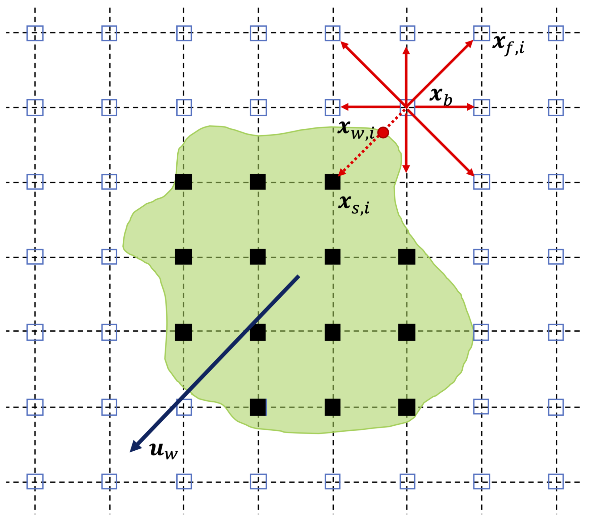
There are many approaches which allow dealing with moving boundaries in LB framework. Here, the one proposed in [49] and further developed in [27] is adopted. This method allows a precise reconstruction of the near-boundary fluid-dynamics fields via reconstructing missing populations through local conserved quantities, such as density and flux , as well as pressure tensor . Figure 1 helps in defining all the missing quantities and catching the populations to be reconstructed at near-boundary fluid nodes.
For every fluid node lying near a solid one, one can determine the subset of velocities which point from the solid to the fluid and, by means of the Grad’s approximation, one can reconstruct missing distribution functions needed during streaming phase. The set of missing populations to be reconstructed before streaming can be defined as follows:
where the pressure tensor can be expanded in its two parts, equilibrium and non-equilibrium, defined as follows:
where the equilibrium part is evaluated by means of the target quantities introduced below while the non-equilibrium may be evaluated by means of velocity gradient referred to the previous iteration. The target velocity can be retrieved by means of a linear interpolation based on neighbor-fluid node velocity and on wall velocity at intersection point , as in Equation (19):
being the number of unknown populations at boundary fluid node, the fluid velocity at node , the solid wall velocity, and the fluid-wall normalized distance . Finally, the target density can be written as the sum of two contributions; the former is related to the standard bounce back rule and the latter related to the solid wall motion:
where and are defined as follows:
being bounced-back distribution functions with and a reference density commonly set equal to the unity. Obviously, in the case of stationary walls, the second row of Equation (21) vanishes to zero, and the target density may be obtained only through a “bounce-back” approach.
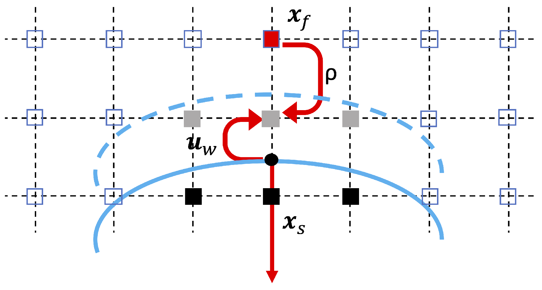
It is worth noting that, during obstacle motion, some nodes can be covered/uncovered by the obstacle passage. In the case of covered node, a fluid node is converted into solid one and no particular treatment is needed for this transformation. On the contrary, when a solid node is uncovered by the obstacle, it has be converted into a fluid one and some handling is needed. More specifically, the so-called refilling procedure can be adopted where density is inherited from a donor fluid node and velocity from moving obstacle, as synthetically reported in Figure 2, and distribution functions are assumed to be equal to equilibrium ones.
Once having clarified the moving boundary treatment, it is important to point out how the FSI interaction is evaluated via integrating the stress tensor along the wetted surface. Thus, the wetted obstacle node stress tensor is evaluated via averaging its value on the neighbor fluid/interface nodes, as in Equation (22).
being the stress tensor at ith wetted solid node, K the number of fluid/interface donor nodes, and the stress tensor at donor node . Finally, the horizontal and vertical components of the forces are the are evaluated as in Equation (23).
where W is the total number of obstacle wetted nodes, and are the stress tensor components along the two main directions, and and are the Lagrangian lengths at the obstacle wetted surface projected along the two main directions x and y. The three stress tensor components can be evaluated in the LBM grid, before the averaging on the obstacle nodes, as in Equation (24):
2.4. The Free-Surface Model
With the aim of considering the multiphase flows of two immiscible fluids with high density ratio, the free surface model is here considered. Throughout this approach, only the denser (and heavier) phase is solved solved within the LB framework (both for BGK and KBC). The two phases interaction are incorporated through specific treatments at interface cells, as explained below. Recently, different free-surface approaches have been developed for LBM [50,51,52,53]. In this work the one developed by Thürey and Rüde [51] is adopted. Thus, with the aim of simulating free-surface evolution, a flag field is introduced to track fluid, interface, and empty cells. For the sake of clarity, the passage from continuous description to the discrete one is briefly reported in Figure 3, where the three considered states are highlighted, namely fluid (F), interface (IF), and gas (G).
Being interface cells partially filled by fluid, the fluid fraction is introduced and defined as , where m is the local mass. Trivially, can range from 0 (gas cells) to 1 (fluid cells). Synthetically, the tracking of the free-surface consists of three steps to be embedded into LB algorithm: (1) computation of the interface motion; (2) boundary conditions at the interface; and (3) re-initialization of the flag field. The first step, the computation of the interface motion, is based on the evaluation of the mass exchanged in between two cells along the allowed directions ; this quantity is proportional to the difference of distribution functions along the involved direction multiplied by a factor defined according to the donor cell type:
All the contributions evaluated according Equation (25) represent the mass variation of the specific interface cell m and they can be summed over the whole set of allowed directions:
After performing the mass exchange process, before the streaming phase, a fictitious boundary condition at interface cells has to be introduced. As stated above, no computations are performed for the empty cells; nevertheless, the interactions between the two phases are included in this step and information coming from the empty cells are supposed to reach the interface cells, where the streaming has to be performed. Therefore, for those cells, starting from the atmospheric reference density (), the missing distribution functions can be computed, at each time step, as follows:
where subscript indicates the lattice direction corresponding to the stencil velocity and indicates the interface density evaluated as , with the surface tension and the local interface curvature. Namely, the interface density is the sum of two contributions, the one related to atmospheric pressure and the one from curvature (Laplace law): , where is the ambient pressure and is the Laplace contribution [52,54]. One can now recall the weakly compressible framework where the LB acts and the pressure and density are linked through the speed of sound: . Thus, with writing the previous equation in terms of density, one can obtain . Equation (27) has to be evaluated for all interface cells which have an empty neighbor along the ith direction. After this reconstruction step, the unknown incoming distribution functions are further reinforced by means of the local free-surface orientation throughout the local normal. After this reconstruction step, the streaming phase is performed for both fluid and interface nodes. Additionally, after the collision phase, every interface cell can be filled or emptied. Thus, the excess/lack of mass occurring at these cells must be computed and redistributed to the neighbor cells. An interface cell is filled and transformed into fluid if the fluid fraction results greater than 1 at the end of the loop, while, on the contrary, it is emptied and converted into gas if this quantity drops below 0. For a filled/emptied cell, the mass excess can be evaluated as follows:
with a tolerance chosen at the beginning of the simulation and fixed to , as in [55]. From Equation (28), one can notice how the mass excess is positive in the case of filled cell, while it is negative for an emptied cell. Finally, the so-computed mass excess has to be distributed to the neighbors by accounting for the direction of the interface normal as a weight:
where is the sum of all the weights , defined as the scalar product . The free-surface normal can be evaluated by means of the fluid fraction gradient, . After the mass redistribution process, the flag of emptied/filled interface cells has to be updated before starting a new time step. The basic principles of free-surface algorithm are synthetically depicted in Figure 4.
3. Model Validation
The two developed solvers were compared with results experimentally retrieved in [32] and later numerically replicated in [33]. The test case is a three-dimensional circular cylinder immersed at constant velocity in a calm water tank. The dimensions of the specimen and of the tank are synthetically reported in Table 1 and depicted in Figure 5.
D is the specimen diameter, is the calm water height, H is the tank height, and W is the tank width. The input parameter is the constant speed of the impacting cylinder, which varies in the range summarized in Table 2 together with the corresponding Reynolds and Froude numbers, defined as per Equation (30).
with D the impacting cylinder diameter, c the submerging speed, the water kinematic viscosity, and g the gravitational acceleration.
The results were compared in terms of slamming coefficient defined in [32] as the ratio between the vertical force and the inertia:
Thus, some preliminary considerations about LB simulations had to be carried out. All the methods here presented are based on a non-dimensional approach; thus, every physical quantity has to be converted according to some conversion factors defined at the beginning of the simulation. For this specific test case, the reference quantities used to define conversion factors are the obstacle diameter D, the water kinematic viscosity , and the water density . The first allows defining the length conversion factor, the second the time one, and the third is used to define the mass conversion factor. Once such quantities were defined, the derived ones could be evaluated accordingly. For example, the calm water height can be written in Lattice Units (LU) starting from the number of points used to discretize the obstacle . The computational domain here simulated perfectly replicates the physical one presented in [32]; however, it can be determined only after having fixed the number of computational points used to discretize the obstacle. After defining the length conversion factor, all lengths could be converted accordingly into the non-dimensional framework. As stated above, the kinematic viscosity in LU, used in LB framework to define the relaxation time as per Equation (5), allows defining the conversion factor for time. Thus, the constant impact speed can be converted into non-dimensional units by means of the two conversion factors defined thus far, the one related to length and the one to time, respectively. It is important to point out that all the non-dimensional numbers such as Re and Fr are not influenced by this change of units; thus, they assume the same value referring to both the physical world and the LB one. Before presenting the results, some more detail about simulation setup are given in the following. Being the obstacle motion driven during the whole simulation, to save computational time, the cylinder was placed one computational grid point above the calm water level. Then, the computational time started and iterations were executed by performing both LBM (either BGK or KBC) and free-surface algorithms. The computational grid was characterized by a set of Cartesian–Eulerian points where the obstacle, defined as a series of Lagrangian points, could move according to the imposed equation of motion. In this specific test case, the obstacle moved at constant vertical speed from the calm water height towards the bottom of the domain. During the simulation, the FSI, which consisted here in evaluating the exchanged forces at boundary in between solid and fluid, was performed every iteration, and after it was sampled with a frequency of 100 Hz during the post processing phase. The stress tensor components were locally evaluated along the contact line and integrated along the whole wetted line to compute the slamming coefficient defined in Equation (31). For the KBC model, both grid sensitivity and Re influence were carried out. Different resolutions were used for the cylinder diameter to highlight the effect of sizing on results, while the Reynolds number was limited definitely below the target one, reported in Table 1. In fact, it was already shown by Zhu et al. [33] that the Re number does not influence the above-mentioned coefficient during process evolution. Moreover, despite being the reference a three-dimensional test case, it was treated in a two-dimensional framework. Table 3 presents the parameters used for the sensitivity analysis.
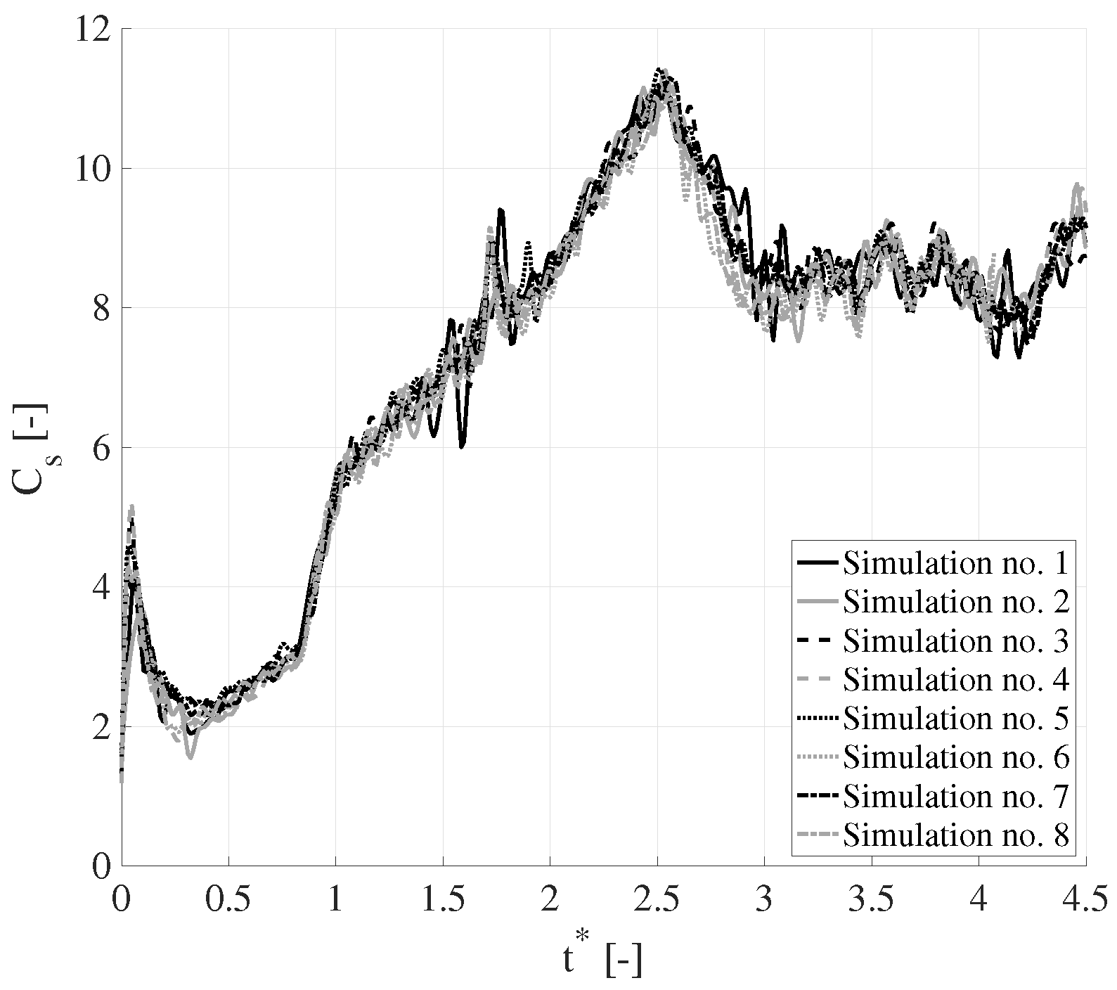
Figure 6 depicts results of slamming coefficient as a function of non dimensional time defined as , with t the time, c the submerging speed, and R the cylinder radius, expressed in LU.
It is worth noting how both Reynolds number and grid resolution slightly affect the slamming coefficient evolution, sampled with a frequency of . However, as easily predicted, the finer is the grid, the better are the results. Referring to Figure 6, the wrinkling tends to vanish with increasing the resolution. For a better understanding of the grid resolution influence, one can consider a magnification of Figure 6 where the first phases of the impact are reported and graphed in Figure 7.
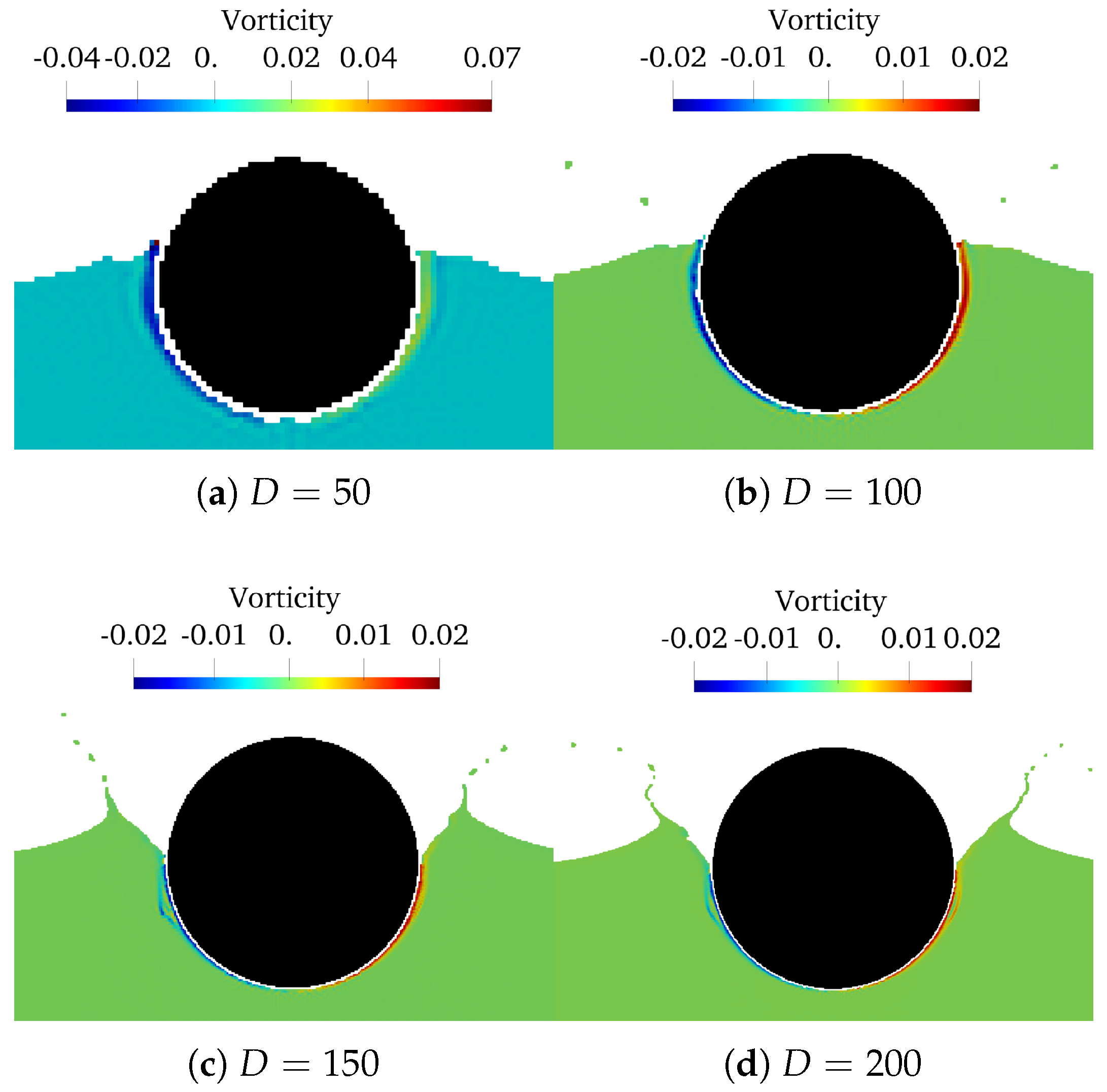
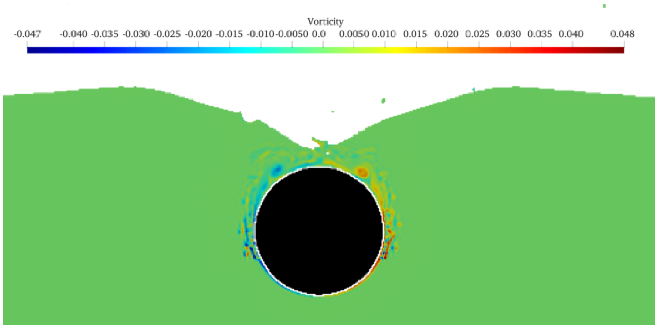
In Figure 7, one can note how the coarser grid tends to underestimate the first peak with respect to the two finer ones, despite being qualitatively comparable when observing the overall trend. Hereafter, the chosen resolution is the one where , which allows achieving appreciable results with saving computational time. To further assess the results, the vorticity plot at for Re = 3660 is reported in Figure 8.
In Figure 7, one can observe how the last two subplots, namely and , practically present the same vorticity distribution in terms of both silhouette and magnitude. Thus, comparing Figure 7 and Figure 8, one can conclude that the wrinkling weakening can be imputed both at the resolution used and to the vorticity level. Moreover, in Figure 8, one can also observe how the last two resolutions present some details in the free-surface silhouette which cannot be highlighted in the reference resolution ; nevertheless, with respect to slamming coefficient, no particular differences arise while considering or , as shown in Figure 6. Thus, in the following analysis, is considered as a reference. In Figure 9, Figure 10 and Figure 11, the computed slamming coefficient is compared with experimental findings in [32] according to operating conditions listed in Table 2. The Reynolds number was reduced by a factor of five to guarantee solver stability. Re independence was already demonstrated, as shown in Figure 6 and Figure 7 and in the literature by [33]; thus, the simulated Re spanned about 12,000–19,000 instead of 64,000–95,000, while no modifications was done with respect to Fr number, which represents the ruling parameter. In other words, to keep the Froude number unchanged, the kinematic viscosity of water can be artificially modified by modifying the Reynolds number.
In Figure 9, Figure 10 and Figure 11, one can observe how the coupled free surface-KBC model results well match the experimental ones presented in the literature; some deviations from experimental data are still present but they can be justified by the use of a two-dimensional stencil, the phenomenon is three-dimensional in principle but it has already been treated in a two-dimensional framework in recent works [33]. It is worth noting how the standard BGK solver without any turbulence model shortly exhibits unstable behavior, without reaching the final time steps, due to the moderate Re regime characteristic of the impact, while the implementation of a Smagorinsky sub-grid model helps in solving this issue with results practically overlapped with the KBC model. Moreover, to better compare results for the two considered solvers, namely KBC and BGK plus Smagorinsky, it is useful to present values for and which are locally adjusted according to flow conditions in the two above mentioned algorithms. More specifically parameter rules the collision phase in the KBC model, according to Equations (13) and (14), while rules the collision operator for the BGK-Smagorinsky model, as per Equations (2) and (8).
Figure 12 and Figure 13 depict similar free-surface distributions, except for some minor discrepancies which arise from an imperfect method matching, and it can be also highlighted how the two turbulence “limiters”, namely and , act on the system. The former shows a non-uniform distribution along the whole domain portion represented in Figure 12, while the latter shows an intensification of sub-grid model influence through in a narrowed area around the obstacle. Moreover, the former varies in a wider range with respect to the latter, which is practically centered around the bulk value defined according the bulk fluid viscosity. Obviously, the twos have a different physical meaning, thus no additional comparison in terms of magnitude values can be performed.
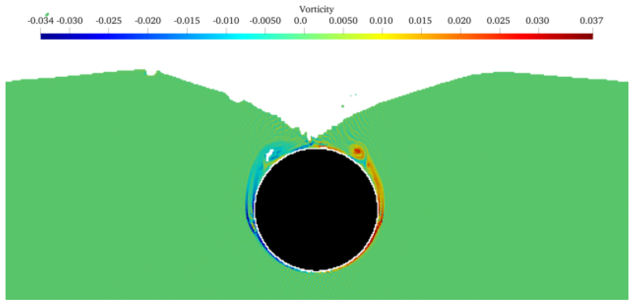
In Figure 14 and Figure 15, one can observe how the two vorticity profiles are practically overlapped, despite being the KBC one “more symmetrical” than the BGK one; white areas included in the fluid domain are representative of the gas phase, which is not solved in the free-surface model, thus no details about vorticity are present. It is worth noting how the magnitude of KBC vorticity is slightly larger than the one of BGK, due to the different approach used while solving turbulent structures. After validating the KBC-free surface and comparing it with a BGK-Smagorinsky solver, as shown in Section 4, a sensitivity analysis was carried out.
4. Results
After validating the proposed method, a sensitivity analysis of slamming coefficient to obstacle aspect ratio was carried out. More specifically, for a circular object such as the one in Section 3, the horizontal radius is equal to the one along the vertical axis . Thus, the effect of the aspect ratio was analyzed and commented to understand the behavior of an impacting ellipsoidal obstacle. The simulation test matrix is reported in Table 4, where Case 3 represents the circular object already analyzed in the previous section. A schematic of the geometrical parameters is reported in Figure 16 where the two radii and are highlighted.
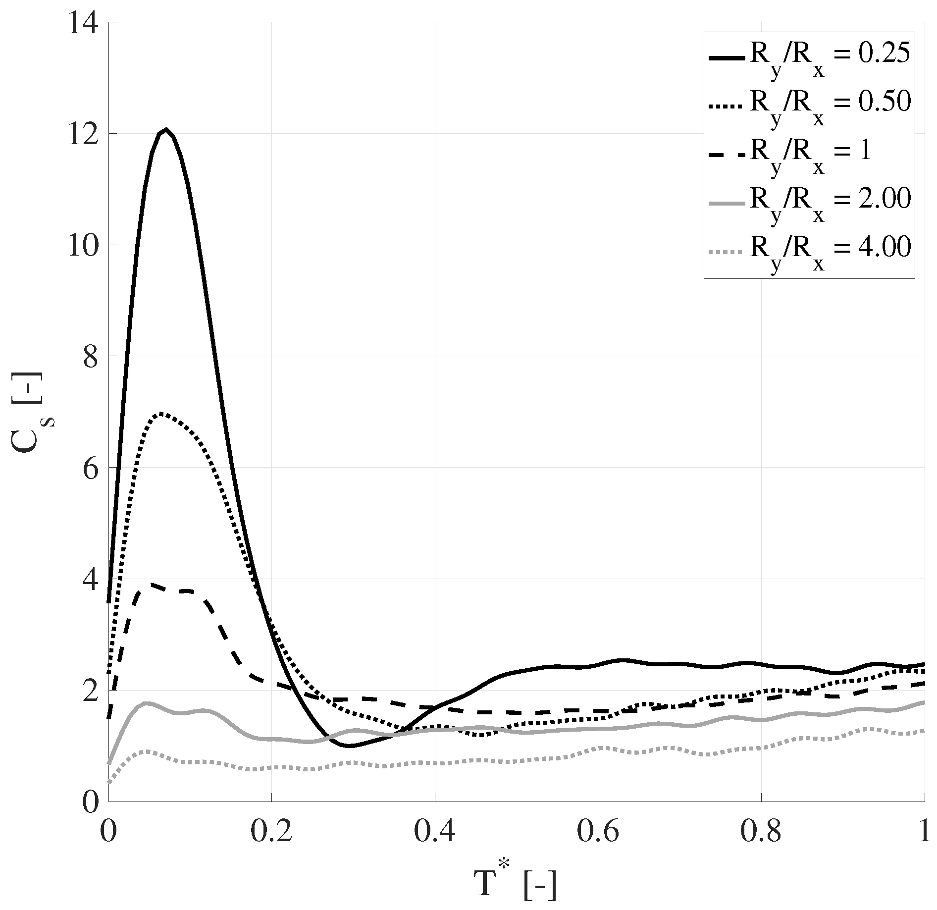
The results in terms of slamming coefficient as a function of the ellipse aspect ratio are briefly reported in Figure 17. It is worth noting how the aspect ratio deeply influences the vertical force component exchanged between the fluid and solid.
In Figure 17, one can notice how, for horizontally aligned ellipses (when ), the slamming coefficient has a really comparable trend except for the initial values and for oscillations amplitude. The asymptotic value, after the fully submerged wedge time—represented by the second peak—tends to be aligned for the considered cases. On the contrary, for vertically aligned ellipses (), the trend does not show the same plateau reference due to an increased submerging time value and the initial value decreases with respect to horizontal obstacles. This is further confirmed by the magnification reported in Figure 18.
In addition, the at first impact time is significantly influenced by the ratio , as one can observe in Figure 19.
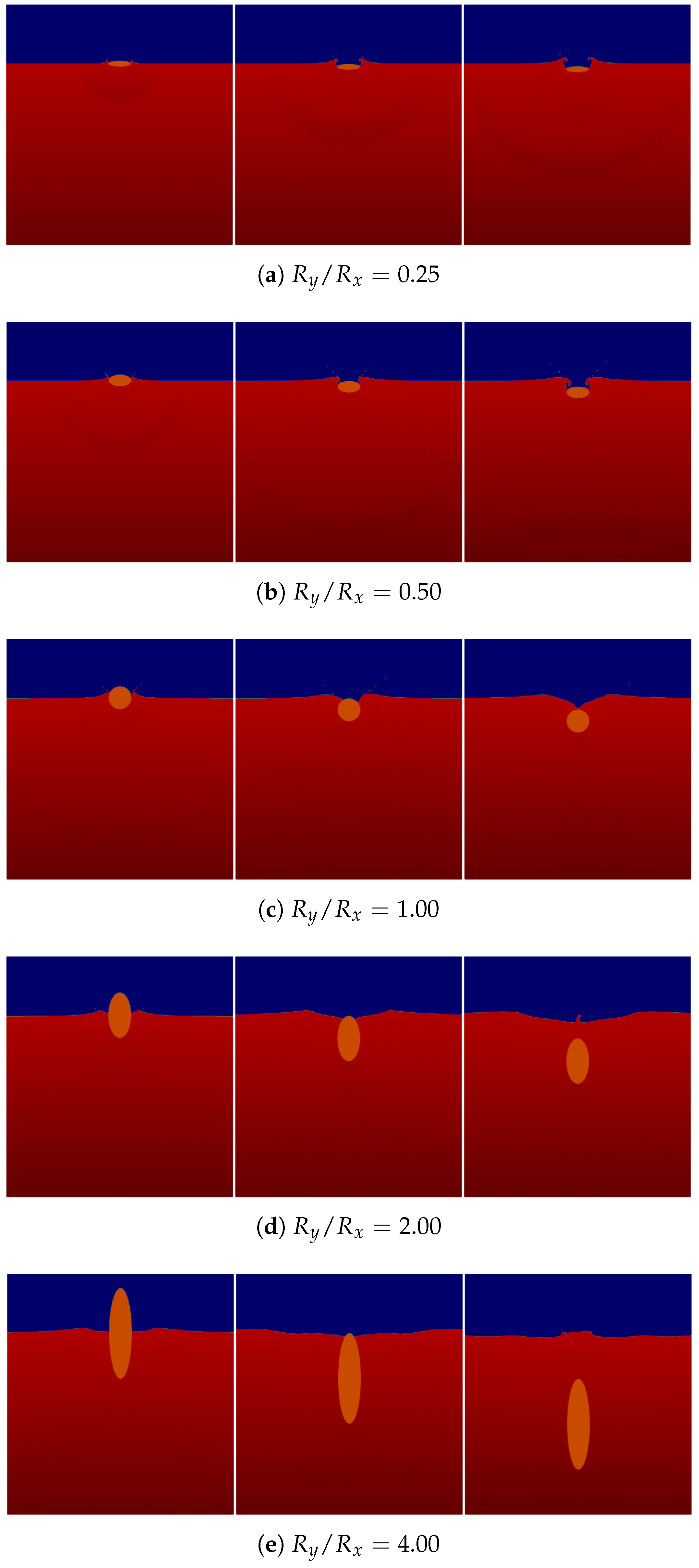
In Figure 19, one can note how the “thinner” the is body along the impact direction, the lower is the slamming coefficient at first impact stages. For a more comprehensive understanding, density plot at different time steps for the considered geometries are reported in Figure 20, where the free-surface silhouette is reported as well.
It is worth noting how the ellipse radii ratio significantly influences the free surface evolution during wedge submerging process. In fact, for thicker bodies, when , there is not complete closure of recirculation wave, while, for thinner ones, when , the body is “fully” surrounded by fluid. Moreover, the submerging process of thick bodies exhibits some circular compression waves, which apparently vanish for thinner ones.
For the sake of clarity, it is useful to introduce a different non-dimensional time, where the reference is the time when the body is theoretically fully submerged. To define such a time, the reference time when the body is fully submerged without considering the pile up is defined as , being the constant submerging speed. Thus, the new dimensional time can be defined as:
Additionally, the slamming coefficient defined in Equation (31) is slightly modified by considering the theoretical wetted diameter instead of the wedge horizontal diameter. Thus, the new slamming coefficient can be defined as follows:
being the instantaneous theoretical wetted diameter defined according Figure 21 and which trivially varies during the obstacle penetration into the water.
The slamming coefficient, reported in Figure 17, can be further reported with respect to the new non-dimensional time.
In Figure 22, one can observe how the new definition for both non-dimensional time and slamming coefficient allows some more considerations. In Figure 22, represents the time when the body is fully submerged without considering the arising pile-up, starting from which the , defined in Equation (33), tends to asymptotic value, which increases with the aspect ratio. Moreover, for negative time, where the body is submerging, it is confirmed how thicker bodies are characterized by higher slamming coefficients.
5. Conclusions
In this study, a coupled KBC-free surface model in the lattice Boltzmann framework was presented and validated. The results were first validated with experimental results already present in the literature and then with a BGK-Smagonrinsky approach, highlighting appreciable results in terms of slamming coefficient in the range of moderate Reynolds number. It was also pointed out how a standard BGK model without any turbulence model is unable to represent the considered phenomenon. The independence from Reynolds number as well as the effect of grid size were shown and commented. The influence of aspect ratio in terms of slamming coefficient was deeply analyzed by pointing out how thick bodies exhibit higher slamming coefficients with respect to thinner ones at first impact stages, but afterwards the trend is opposite with thinner bodies characterized by higher , due to the complete closure of the recirculation wave.
Summarizing, this study aimed at demonstrating the effectiveness of a coupled KBC-free surface model to deal with impacting objects on free surfaces at moderate Reynolds number. The use of KBC approach allows avoiding the introduction of a turbulence model, being such a framework capable of locally adjusting the solution according to a limiter. Very good results were obtained for relatively high Reynolds as well, due to the intrinsic capability of KBC to locally adjust the solution. These results open the door to further developments such as introducing free falling obstacles with embedding the equation of motion.
Funding
This work was supported by the Italian Ministry of Education, University and Research under PRIN grant No. 20154EHYW9 “Combined numerical and experimental methodology for fluid structure interaction in free surface flows under impulsive loading”.
Conflicts of Interest
The author declares no conflict of interest.
References
- Faltinsen, O.M. Hydroelastic slamming. J. Mar. Sci. Technol. 2000, 5, 49–65. [Google Scholar] [CrossRef]
- Facci, A.L.; Panciroli, R.; Ubertini, S.; Porfiri, M. Assessment of PIV-based analysis of water entry problems through synthetic numerical datasets. J. Fluids Struct. 2015, 55, 484–500. [Google Scholar] [CrossRef] [Green Version]
- Panciroli, R.; Biscarini, C.; Falcucci, G.; Jannelli, E.; Ubertini, S. Live monitoring of the distributed strain field in impulsive events through fiber Bragg gratings. J. Fluids Struct. 2016, 61, 60–75. [Google Scholar] [CrossRef]
- Erturk, A.; Delporte, G. Underwater thrust and power generation using flexible piezoelectric composites: An experimental investigation toward self-powered swimmer-sensor platforms. Smart Mater. Struct. 2011, 20, 125013. [Google Scholar] [CrossRef]
- Batra, R.; Porfiri, M.; Spinello, D. Review of modeling electrostatically actuated microelectromechanical systems. Smart Mater. Struct. 2007, 16, R23. [Google Scholar] [CrossRef]
- De Tullio, M.; Cristallo, A.; Balaras, E.; Verzicco, R. Direct numerical simulation of the pulsatile flow through an aortic bileaflet mechanical heart valve. J. Fluid Mech. 2009, 622, 259–290. [Google Scholar] [CrossRef] [Green Version]
- Wang, L.; Currao, G.M.; Han, F.; Neely, A.J.; Young, J.; Tian, F.B. An immersed boundary method for fluid–structure interaction with compressible multiphase flows. J. Comput. Phys. 2017, 346, 131–151. [Google Scholar] [CrossRef] [Green Version]
- Calderer, A.; Guo, X.; Shen, L.; Sotiropoulos, F. Fluid—Structure interaction simulation of floating structures interacting with complex, large-scale ocean waves and atmospheric turbulence with application to floating offshore wind turbines. J. Comput. Phys. 2018, 355, 144–175. [Google Scholar] [CrossRef]
- Ren, Z.; Wang, Z.; Stern, F.; Judge, C.; Ikeda-Gilbert, C. Vertical Water Entry of a Flexible Wedge into Calm Water: A Fluid-Structure Interaction Experiment. J. Ship Res. 2019, 63, 41–55. [Google Scholar] [CrossRef]
- Facci, A.L.; Falcucci, G.; Agresta, A.; Biscarini, C.; Jannelli, E.; Ubertini, S. Fluid Structure Interaction of Buoyant Bodies with Free Surface Flows: Computational Modelling and Experimental Validation. Water 2019, 11, 1048. [Google Scholar] [CrossRef] [Green Version]
- Panciroli, R.; Abrate, S.; Minak, G.; Zucchelli, A. Hydroelasticity in water-entry problems: Comparison between experimental and SPH results. Compos. Struct. 2012, 94, 532–539. [Google Scholar] [CrossRef]
- Khayyer, A.; Gotoh, H.; Falahaty, H.; Shimizu, Y. An enhanced ISPH–SPH coupled method for simulation of incompressible fluid—Elastic structure interactions. Comput. Phys. Commun. 2018, 232, 139–164. [Google Scholar] [CrossRef]
- Owen, D.; Leonardi, C.; Feng, Y. An efficient framework for fluid–structure interaction using the lattice Boltzmann method and immersed moving boundaries. Int. J. Numer. Methods Eng. 2011, 87, 66–95. [Google Scholar] [CrossRef]
- De Rosis, A. Ground-induced lift enhancement in a tandem of symmetric flapping wings: Lattice Boltzmann-immersed boundary simulations. Comput. Struct. 2015, 153, 230–238. [Google Scholar] [CrossRef]
- Aureli, M.; Prince, C.; Porfiri, M.; Peterson, S.D. Energy harvesting from base excitation of ionic polymer metal composites in fluid environments. Smart Mater. Struct. 2009, 19, 015003. [Google Scholar] [CrossRef]
- Panciroli, R. Hydroelastic impacts of deformable wedges. In Dynamic Failure of Composite and Sandwich Structures; Springer: Dordrecht, The Netherlands, 2013; pp. 1–45. [Google Scholar]
- Panciroli, R.; Porfiri, M. Analysis of hydroelastic slamming through particle image velocimetry. J. Sound Vib. 2015, 347, 63–78. [Google Scholar] [CrossRef]
- Panciroli, R.; Ubertini, S.; Minak, G.; Jannelli, E. Experiments on the Dynamics of Flexible Cylindrical Shells Impacting on a Water Surface. Exp. Mech. 2015, 55, 1537–1550. [Google Scholar] [CrossRef]
- Panahi, R. Simulation of water-entry and water-exit problems using a moving mesh algorithm. J. Theor. Appl. Mech. 2012, 42, 79–92. [Google Scholar] [CrossRef] [Green Version]
- Cheon, J.S.; Jang, B.S.; Yim, K.H.; Lee, H.D.; Koo, B.Y.; Ju, H. A study on slamming pressure on a flat stiffened plate considering fluid–structure interaction. J. Mar. Sci. Technol. 2016, 21, 309–324. [Google Scholar] [CrossRef]
- Zhao, X.; Gao, Y.; Cao, F.; Wang, X. Numerical modeling of wave interactions with coastal structures by a constrained interpolation profile/immersed boundary method. Int. J. Numer. Methods Fluids 2016, 81, 265–283. [Google Scholar] [CrossRef]
- Falcucci, G.; Aureli, M.; Ubertini, S.; Porfiri, M. Transverse harmonic oscillations of laminae in viscous fluids: A lattice Boltzmann study. Philos. Trans. R. Soc. A Math. Phys. Eng. Sci. 2011, 369, 2456–2466. [Google Scholar] [CrossRef] [Green Version]
- De Rosis, A.; Falcucci, G.; Ubertini, S.; Ubertini, F.; Succi, S. Lattice Boltzmann analysis of fluid-structure interaction with moving boundaries. Commun. Comput. Phys. 2013, 13, 823–834. [Google Scholar] [CrossRef]
- De Rosis, A.; Falcucci, G.; Porfiri, M.; Ubertini, F.; Ubertini, S. Hydroelastic analysis of hull slamming coupling lattice Boltzmann and finite element methods. Comput. Struct. 2014, 138, 24–35. [Google Scholar] [CrossRef]
- De Rosis, A.; Falcucci, G.; Ubertini, S.; Ubertini, F. Aeroelastic study of flexible flapping wings by a coupled lattice Boltzmann-finite element approach with immersed boundary method. J. Fluids Struct. 2014, 49, 516–533. [Google Scholar] [CrossRef]
- Zarghami, A.; Falcucci, G.; Jannelli, E.; Succi, S.; Porfiri, M.; Ubertini, S. Lattice Boltzmann modeling of water entry problems. Int. J. Mod. Phys. C 2014, 25, 1441012. [Google Scholar] [CrossRef]
- Dorschner, B.; Chikatamarla, S.S.; Bösch, F.; Karlin, I.V. Grad’s approximation for moving and stationary walls in entropic lattice Boltzmann simulations. J. Comput. Phys. 2015, 295, 340–354. [Google Scholar] [CrossRef]
- Dorschner, B.; Chikatamarla, S.S.; Karlin, I.V. Entropic multirelaxation-time lattice Boltzmann method for moving and deforming geometries in three dimensions. Phys. Rev. E 2017, 95, 063306. [Google Scholar] [CrossRef] [Green Version]
- Di Ilio, G.; Dorschner, B.; Bella, G.; Succi, S.; Karlin, I.V. Simulation of turbulent flows with the entropic multirelaxation time lattice Boltzmann method on body-fitted meshes. J. Fluid Mech. 2018, 849, 35–56. [Google Scholar] [CrossRef]
- Karlin, I.V.; Bösch, F.; Chikatamarla, S. Gibbs’ principle for the lattice-kinetic theory of fluid dynamics. Phys. Rev. E 2014, 90, 031302. [Google Scholar] [CrossRef] [PubMed]
- Thuerey, N. Physically based Animation of Free Surface Flows with the Lattice Boltzmann Method. Ph.D. Thesis, University of Erlangen, Erlangen, Germany, 2007. [Google Scholar]
- Miao, G. Hydrodynamic Forces and Dynamic Responses of Circular Cylinders in Wave Zones. Ph.D. Thesis, Division of Marine Hydrodynamics, The Norwegian Institute of Technology, University of Trondheim, Trondheim, Norway, 1988. [Google Scholar]
- Zhu, X.; Faltinsen, O.M.; Hu, C. Water Entry and Exit of a Horizontal Circular Cylinder. J. Offshore Mech. Arct. Eng. 2006, 129, 253–264. [Google Scholar] [CrossRef]
- Sagaut, P. Toward advanced subgrid models for Lattice-Boltzmann-based Large-eddy simulation: Theoretical formulations. Comput. Math. Appl. 2010, 59, 2194–2199. [Google Scholar] [CrossRef] [Green Version]
- Guo, M.; Tang, X.; Su, Y.; Li, X.; Wang, F. Applications of Three-Dimensional LBM-LES Combined Model for Pump Intakes. Commun. Comput. Phys. 2018, 24, 104–122. [Google Scholar] [CrossRef] [Green Version]
- Benzi, R.; Succi, S.; Vergassola, M. The Lattice Boltzmann Equation: Theory and Applications. Phys. Rep. 1992, 222, 145–197. [Google Scholar] [CrossRef]
- Karlin, I.; Ferrante, A.; Öttinger, H. Perfect entropy functions of the Lattice Boltzmann method. Europhys. Lett. 1999, 47, 182–188. [Google Scholar] [CrossRef] [Green Version]
- Succi, S. The Lattice Boltzmann Equation: For Complex States of Flowing Matter; Oxford University Press: Oxford, UK, 2018. [Google Scholar]
- Xie, C.; Zhang, J.; Bertola, V.; Wang, M. Lattice Boltzmann modeling for multiphase viscoplastic fluid flow. J. Non-Newton. Fluid Mech. 2016, 234, 118–128. [Google Scholar] [CrossRef]
- Di Ilio, G.; Chiappini, D.; Ubertini, S.; Bella, G.; Succi, S. Fluid flow around NACA 0012 airfoil at low-Reynolds numbers with hybrid lattice Boltzmann method. Comput. Fluids 2018, 166, 200–208. [Google Scholar] [CrossRef]
- Di Ilio, G.; Chiappini, D.; Ubertini, S.; Bella, G.; Succi, S. A moving-grid approach for fluid–structure interaction problems with hybrid lattice Boltzmann method. Comput. Phys. Commun. 2019, 234, 137–145. [Google Scholar] [CrossRef]
- Aidun, C.K.; Clausen, J.R. Lattice-Boltzmann method for complex flows. Ann. Rev. Fluid Mech. 2010, 42, 439–472. [Google Scholar] [CrossRef]
- Sbragaglia, M.; Benzi, R.; Biferale, L.; Succi, S.; Sugiyama, K.; Toschi, F. Generalized lattice Boltzmann method with multirange pseudopotential. Phys. Rev. E 2007, 75, 026702. [Google Scholar] [CrossRef] [Green Version]
- Fernandino, M.; Beronov, K.; Ytrehus, T. Large eddy simulation of turbulent open duct flow using a lattice Boltzmann approach. Math. Comput. Simul. 2009, 79, 1520–1526. [Google Scholar] [CrossRef]
- Bösch, F.; Chikatamarla, S.S.; Karlin, I.V. Entropic multirelaxation lattice Boltzmann models for turbulent flows. Phys. Rev. E 2015, 92, 043309. [Google Scholar] [CrossRef] [PubMed]
- Dorschner, B.; Frapolli, N.; Chikatamarla, S.S.; Karlin, I.V. Grid refinement for entropic lattice Boltzmann models. Phys. Rev. E 2016, 94, 053311. [Google Scholar] [CrossRef] [PubMed] [Green Version]
- Dorschner, B.; Bösch, F.; Chikatamarla, S.S.; Boulouchos, K.; Karlin, I.V. Entropic multi-relaxation time lattice Boltzmann model for complex flows. J. Fluid Mech. 2016, 801, 623–651. [Google Scholar] [CrossRef]
- Kupershtokh, A.; Medvedev, D.; Karpov, D. On equations of state in a lattice Boltzmann method. Comput. Math. Appl. 2009, 58, 965–974. [Google Scholar] [CrossRef] [Green Version]
- Chikatamarla, S.S.; Ansumali, S.; Karlin, I.V. Grad’s approximation for missing data in lattice Boltzmann simulations. EPL Europhys. Lett. 2006, 74, 215. [Google Scholar] [CrossRef] [Green Version]
- Ginzburg, I.; Steiner, K. A free-surface lattice Boltzmann method for modelling the filling of expanding cavities by Bingham fluids. Philos. Trans. R. Soc. Lond. A 2002, 360, 453–466. [Google Scholar] [CrossRef]
- Thürey, N.; Rüde, U. Stable free surface flows with the lattice Boltzmann method on adaptively coarsened grids. Comput. Vis. Sci. 2009, 12, 247–263. [Google Scholar] [CrossRef]
- Körner, C.; Thies, M.; Hofmann, T.; Thürey, N.; Rüde, U. Lattice Boltzmann model for free surface flow for modeling foaming. J. Stat. Phys. 2005, 121, 179–196. [Google Scholar] [CrossRef]
- Janssen, C.; Krafczyk, M. A lattice Boltzmann approach for free-surface-flow simulations on non-uniform block-structured grids. Comput. Math. Appl. 2010, 59, 2215–2235. [Google Scholar] [CrossRef] [Green Version]
- Anderl, D.; Bogner, S.; Rauh, C.; Rüde, U.; Delgado, A. Free surface lattice Boltzmann with enhanced bubble model. Comput. Math. Appl. 2014, 67, 331–339. [Google Scholar] [CrossRef]
- Thürey, N.; Körner, C.; Rüde, U. Interactive Free Surface Fluids with the Lattice Boltzmann Method; Technical Report05-4; University of Erlangen-Nuremberg: Erlangen, Germany, 2005. [Google Scholar]
Figure 1.
Obstacle definition into fluid domain. Empty squares represent the fluid nodes, filled squares belong to the obstacle; the red filled circle represents the exact wall position along the ith lattice direction. Continuous red arrows represent the known populations, while the dashed ones represent the ones to be reconstructed before streaming.

Figure 2.
Schematic representation of refilling procedure. The obstacle, initially located at the dashed cyan line (new position is the solid cyan line) frees some nodes, the gray filled ones, which belonged to the solid. Their new fluid-dynamics properties are copied from both red filled fluid node and solid one .

Figure 3.
Three states treatment for free-surface model: fluid, interface, and gas.

Figure 4.
Schematic of the free-surface update cell procedure.

Figure 5.
Representation (not to scale) of the computational domain used for validation.

Figure 6.
Slamming coefficient as a function of non-dimensional time for the sensitivity matrix reported in Table 3. Black curves are related to low Re, gray ones to high Re. Solid line refers to , dashed ones to , dotted ones to , and dash-dotted ones to .
Figure 6.
Slamming coefficient as a function of non-dimensional time for the sensitivity matrix reported in Table 3. Black curves are related to low Re, gray ones to high Re. Solid line refers to , dashed ones to , dotted ones to , and dash-dotted ones to .

Figure 7.
Magnification of Figure 6 referring to the first impact phases. Black curves are related to low Re, gray ones to high Re. Solid line refers to , dashed ones to , dotted ones to and dash-dotted ones to .
Figure 7.
Magnification of Figure 6 referring to the first impact phases. Black curves are related to low Re, gray ones to high Re. Solid line refers to , dashed ones to , dotted ones to and dash-dotted ones to .

Figure 8.
Vorticity plot for different resolution at for Re = 3660: (a–d) the obstacle diameter from to , respectively.
Figure 8.
Vorticity plot for different resolution at for Re = 3660: (a–d) the obstacle diameter from to , respectively.

Figure 9.
Comparison between experimental results presented by [32] and numerical model at . Black dotted line represents experimental findings, solid red line the KBC results, magenta line the BGK without turbulence model, and the blue curve represents the BGK with Smagorinsky sub-grid model.
Figure 9.
Comparison between experimental results presented by [32] and numerical model at . Black dotted line represents experimental findings, solid red line the KBC results, magenta line the BGK without turbulence model, and the blue curve represents the BGK with Smagorinsky sub-grid model.

Figure 10.
Comparison between experimental results presented by [32] and numerical model at . Black dotted line represents experimental findings, solid red line the KBC results, magenta line the BGK without turbulence model, and the blue curve represents the BGK with Smagorinsky sub-grid model.
Figure 10.
Comparison between experimental results presented by [32] and numerical model at . Black dotted line represents experimental findings, solid red line the KBC results, magenta line the BGK without turbulence model, and the blue curve represents the BGK with Smagorinsky sub-grid model.

Figure 11.
Comparison between experimental results presented by [32] and numerical model at . Black dotted line represents experimental findings, solid red line the KBC results, magenta line the BGK without turbulence model, and the blue curve represents the BGK with Smagorinsky sub-grid model.
Figure 11.
Comparison between experimental results presented by [32] and numerical model at . Black dotted line represents experimental findings, solid red line the KBC results, magenta line the BGK without turbulence model, and the blue curve represents the BGK with Smagorinsky sub-grid model.

Figure 12.
parameter when the obstacle is completely submerged at for .

Figure 13.
parameter when the obstacle is completely submerged at for .

Figure 14.
Vorticity profile for KBC method when the obstacle is completely submerged at for .

Figure 15.
Vorticity profile for BGK method when the obstacle is completely submerged at for .

Figure 16.
Schematic representation of the ellipsoidal obstacle with the sensitivity analysis parameters.
Figure 16.
Schematic representation of the ellipsoidal obstacle with the sensitivity analysis parameters.

Figure 17.
Slamming coefficient as a function of the ellipse aspect ratio. Solid black line represents aspect ratio of 0.25, dotted black line 0.5, dashed black line the circular obstacle with , solid light gray line the aspect ratio of 2.0, and dotted light gray line the largest aspect ratio of 4.0.

Figure 18.
Magnification up to of the slamming coefficient as a function of the ellipse aspect ratio. Solid black line represents aspect ratio of 0.25, dotted black line 0.5, dashed black line the circular obstacle with , solid light gray line the aspect ratio of 2.0, and dotted light gray line the largest aspect ratio of 4.0.

Figure 19.
Slamming coefficient at first impact time as a function of aspect ratio.

Figure 20.
Density evolution at different non-dimensional times for different ellipse geometry. The three snapshots for ever radii ratio represent half of wedge wetted, full wetted wedge, and three-quarters of wetted wedge, respectively. The three obstacle penetrations correspond to the same non-dimensional times, more specifically 1.05, 2.10, and 3.10, respectively.

Figure 21.
Schematic representation of the theoretical instantaneous wetted diameter used in Equation (33).
Figure 21.
Schematic representation of the theoretical instantaneous wetted diameter used in Equation (33).

Figure 22.
Evolution of the new slamming coefficient as a function of the non-dimensional time. Solid black line represents aspect ratio of 0.25, dotted black line 0.5, dashed black line the circular obstacle with , solid light gray line the aspect ratio of 2.0, and dotted light gray line the largest aspect ratio of 4.0.


Table 1.
Input parameters for model validation.
| 0.125 | 28.0 | 2.5 | 1.0 |
Table 2.
Cylinder velocity and corresponding Reynolds and Froude numbers.
| Case | Re | ||
|---|---|---|---|
| 1 | 0.5124 | 64050 | 0.4628 |
| 2 | 0.6390 | 79875 | 0.5772 |
| 3 | 0.7600 | 95000 | 0.6865 |
Table 3.
Test matrix for sensitivity analysis at constant . means that all the quantities are expressed in non-dimensional units characteristic of the LB framework.
Table 3.
Test matrix for sensitivity analysis at constant . means that all the quantities are expressed in non-dimensional units characteristic of the LB framework.
| Simlation No. | ||||
|---|---|---|---|---|
| 1 | 50 | 11,200 × 1000 | 0.00440 | 366 |
| 2 | 50 | 11,200 × 1000 | 0.00044 | 3660 |
| 3 | 100 | 22,400 × 2000 | 0.00880 | 366 |
| 4 | 100 | 22,400 × 2000 | 0.00088 | 3660 |
| 5 | 150 | 33,600 × 3000 | 0.01320 | 366 |
| 6 | 150 | 33,600 × 3000 | 0.00132 | 3660 |
| 7 | 200 | 40,000 × 4000 | 0.01760 | 366 |
| 8 | 200 | 40,000 × 4000 | 0.00176 | 3660 |
Table 4.
Aspect ratio configurations for ellipsoidal obstacle: and .
| Simulation No. | |
|---|---|
| 1 | 0.25 |
| 2 | 0.50 |
| 3 | 1.00 |
| 4 | 2.00 |
| 5 | 4.00 |
© 2020 by the author. Licensee MDPI, Basel, Switzerland. This article is an open access article distributed under the terms and conditions of the Creative Commons Attribution (CC BY) license (http://creativecommons.org/licenses/by/4.0/).
Share and Cite
MDPI and ACS Style
Chiappini, D. Fluid Structure Interaction of 2D Objects through a Coupled KBC-Free Surface Model. Water 2020, 12, 1212. https://doi.org/10.3390/w12041212
AMA Style
Chiappini D. Fluid Structure Interaction of 2D Objects through a Coupled KBC-Free Surface Model. Water. 2020; 12(4):1212. https://doi.org/10.3390/w12041212
Chicago/Turabian StyleChiappini, Daniele. 2020. "Fluid Structure Interaction of 2D Objects through a Coupled KBC-Free Surface Model" Water 12, no. 4: 1212. https://doi.org/10.3390/w12041212
Note that from the first issue of 2016, this journal uses article numbers instead of page numbers. See further details here.