Environmental Control on Transpiration: A Case Study of a Desert Ecosystem in Northwest China

Abstract

Arid and semi-arid ecosystems represent a crucial but poorly understood component of the global water cycle. Taking a desert ecosystem as a case study, we measured sap flow in three dominant shrub species and concurrent environmental variables over two mean growing seasons. Commercially available gauges (Flow32 meters) based on the constant power stem heat balance (SHB) method were used. Stem-level sap flow rates were scaled up to stand level to estimate stand transpiration using the species-specific frequency distribution of stem diameter. We found that variations in stand transpiration were closely related to changes in solar radiation (R_s), air temperature (T), and vapor pressure deficit (VPD) at the hourly scale. Three factors together explained 84% and 77% variations in hourly stand transpiration in 2014 and 2015, respectively, with R_s being the primary driving force. We observed a threshold control of VPD (~2 kPa) on stand transpiration in two-year study periods, suggesting a strong stomatal regulation of transpiration under high evaporative demand conditions. Clockwise hysteresis loops between diurnal transpiration and T and VPD were observed and exhibited seasonal variations. Both the time lags and refill and release of stem water storage from nocturnal sap flow were possible causes for the hysteresis. These findings improve the understanding of environmental control on water flux of the arid and semi-arid ecosystems and have important implications for diurnal hydrology modelling.

1. Introduction

Arid and semi-arid regions covering about 40% of the terrestrial land surface are highly vulnerable to climate change [1]. Evaluating hydrological response to continuous warming and altered precipitation pattern in these regions largely depends on an accurate estimation of evapotranspiration (ET), especially plant transpiration which can be a large contributor of ET, depending on the ecosystem type [2,3]. Sap flow, an indicator of water transport in the plant xylem, provides species-specific estimates of transpiration rate at the whole tree level and can be scaled up to stand level using the appropriate scaling method [4]. During past four decades, sap flow has been widely used to investigate response of transpiration and canopy conductance to environment variables at both daily and sub-daily temporal scales [5], to characterize spatial heterogeneity of water fluxes within stands [6,7], and to quantify the ecosystem water budget [8,9]. However, prior studies heavily focused on humid forest ecosystems, with few sap flow field studies in arid and semi-arid ecosystems. What is the primary driving force for transpiration in a water-limited ecosystem at sub-daily scale? To what extent is transpiration controlled by environment variables in these ecosystems? Are there species-specific differences in the responses? These questions need to be addressed to improve our understanding of the water, energy and carbon exchange between vegetation and atmosphere, accurate long-term hydrologic modelling, and assess ecosystem adaption in the framework of climate change in arid and semi-arid regions.

Environmental variables that may affect transpiration include solar radiation (R_s), air temperature (T), vapor pressure deficit (VPD), relative humidity (RH), wind speed (u), soil moisture (θ), soil temperature (T_s), and precipitation (P). Huang et al. [10] reported that sap flow of the Salix psammophila living in a semi-arid environment in northwestern China was positively related to net radiation (R_n), T, and u, but negatively related to RH. They further analyzed water resources of the S. psammophila using a correlation analysis and multiple linear regression and found that Salix bushes can use both soil water and groundwater for transpiration. Zheng et al. [11] found that an increase in reference evapotranspiration (ET₀), PAR, VPD, and T resulted in an exponential increase in transpiration of the Haloxylon ammodendron (C. A. Mey.) (H. ammodendron), a dominant desert species. Ma et al. [12] reported that sap flow from four typical species of shelter forest in the desert area exhibited a linear relationship with VPD. Shen et al. [13] reported that the sap flow of the Populus gansuensis linearly increased with R_s, and logarithmically increased with VPD and T. All these studies indicate that the response of transpiration to environmental variables is climate- and ecosystem-specific and more research is required to better understand environmental control on transpiration. In addition, diurnal hysteresis between transpiration and environmental variables has been reported in different ecosystems [14,15,16,17]. Both transpiration and environmental variables exhibit diurnal changes, reaching peaks at different times and resulting in a hysteresis behavior. Such hysteresis is usually characterized by the looping pattern when measured transpiration time series is plotted against the relevant environmental variables over the course of one day. Plausible explanations include abiotic (such as time lag between radiation and VPD) and biotic factors (such as stem water storage, soil water potential) [15,18]. Investigating the hysteric phenomenon and revealing the underlying causes would help to understand the relations and interactions between vegetation and its surrounding environment [18].

The H. ammodendron shrubland is extensively distributed in arid regions of China and plays a crucial role in stabilizing sand dunes and protecting oases from desertification [19]. With the development of irrigated agriculture and rapid population growth in the oasis, over-exploration of water resources has resulted in serious environmental degradations, including a gradually fall of the groundwater table, soil salinization, and desertification [20]. All these environmental problems are threatening the survival of the shrubland. Previous studies have examined the response of the photosynthetic traits and physiological characteristics on enhanced precipitation, nitrogen deposition, and drought stress [21,22], analyzed root distribution characteristics [19], revealed biomass allocation [23], and quantified interactions between canopies and the atmosphere [24]. However, a comprehensive analysis of the relationships between stand transpiration and key environmental variables is still limited.

In the current study, we measured stem sap flow from three dominant species of the H. ammodendron shrubland and related environmental variables over the two main growing seasons. We aimed: (i) to clarify the diurnal course of stand transpiration of the selected shrubland; (ii) to explore relationships between transpiration and key environmental variables; and (iii) to reveal hysteresis of transpiration and explore possible causes.

2. Material and Methods

2.1. Site Description

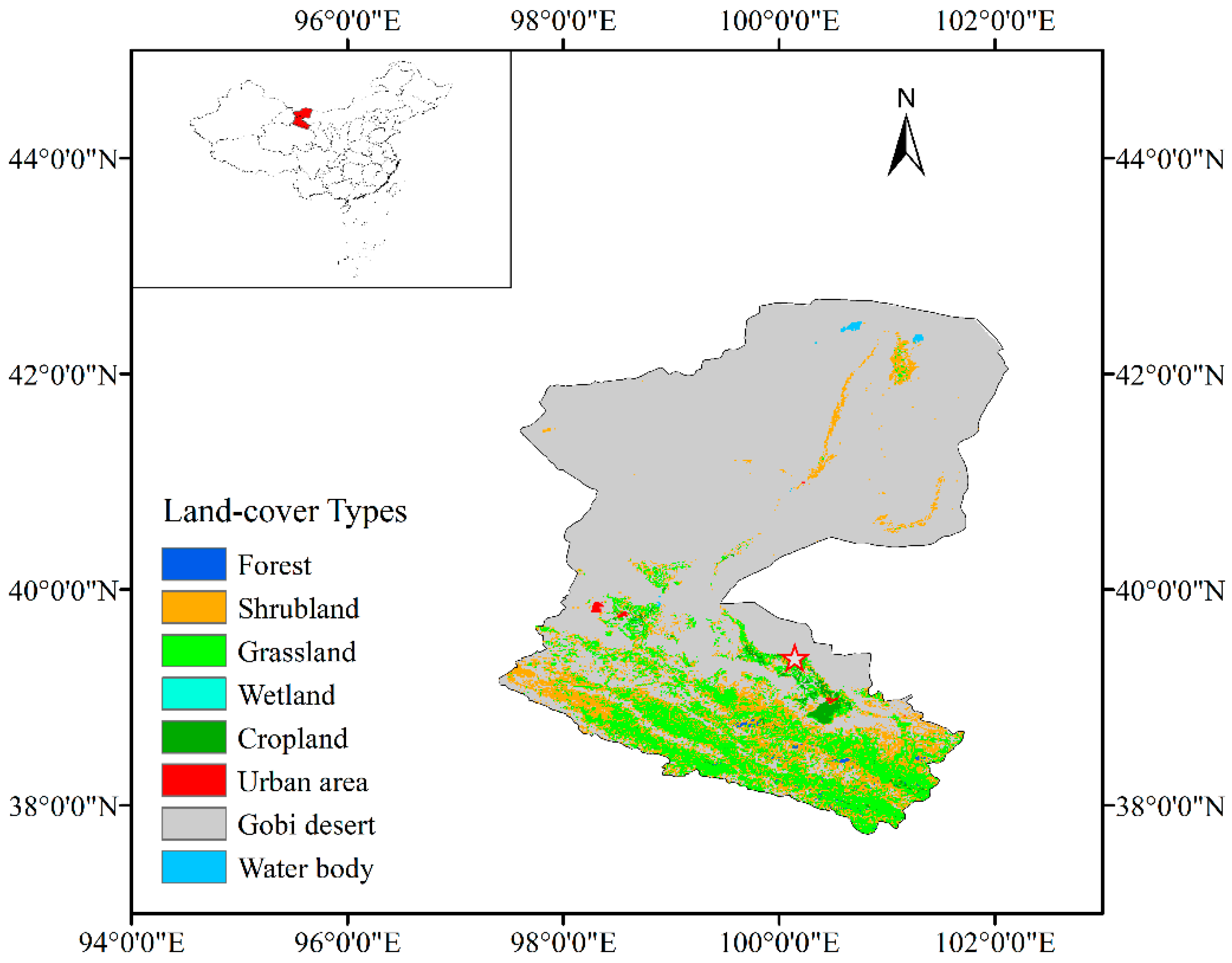
We conducted field experiments within an oasis-desert ecotone in the middle of the Heihe River Basin, Northwestern China (100°08’48’’ E, 39°22’07’’ N, elevation 1386 m) (Figure 1). The climate in this area is characterized by a typical continental and arid temperate climate with dry and hot summers and cold winters. An analysis of a ten-year meteorological station records (2005−2014) showed that the annual averaged air temperature ranges from −26 °C in January to 39 °C in July, with a mean value of 9 °C; the annual mean precipitation is about 124 mm, with is about 80% of the annual total fall between June and September; the daily averaged sunshine duration is about 8.3 h. The groundwater table in the study area ranged from 4.15 m to 4.29 m during the measuring period.

2.2. Vegetation Measurement

A representative plot (50 × 50 m) of H. ammodendron shrubland was selected to conduct vegetation and sap flow measurements. Vegetation within the study plot is characterized by an open shrub canopy consisting of H. ammodendron, Calligonum mongolicum (Turcz.) (C. mongolicum), Nitraria tangutorum (Bobr.) (N. tangutorum), and other shrub and subshrub species. During the intensive experimental period in 2014 (DOY (day of year) 196−222), we measured basal diameter (5 cm above the ground), height, crown area, leaf area, and stand density. Details on vegetation survey and stand characteristics can be found in our previous study [24].

2.3. Environmental Measurements

We constructed a standard automatic weather station within the study plot to measure incoming solar radiation (R_s, W/m²; CNR4, Kipp & Zonen, Delft, Netherlands), photosynthetically active radiation (PAR, μmol/m²/s; LI-190SB, Li-Cor., Lincoln, NE, USA), air temperature (T, °C; HMP155A, Vaisala, Helsinki, Finland), relative humidity (RH, %; HMP155A, Vaisala, Helsinki, Finland), wind speed (u, m/s; 1405-PK-052, Gill Instruments Ltd., Lymington, UK), and precipitation (P, mm; TE525, Texas Electronics Inc., Dallas, TX, USA). Soil temperature (T_s, °C) and soil moisture (θ, m³/m³) were measured at six depths (10, 20, 40, 60, 80, and 120 cm) using thermistor probes (109-L, Campbell Scientific Inc., Logan, UT, USA) and time domain reflectometers (CS616, Campbell Scientific Inc., Logan, UT, USA), respectively. All the environmental variables were recorded at 30-min intervals using a data logger (CR1000, Campbell Scientific Inc., Logan, UT, USA). Vapor pressure deficit (VPD, kPa) was calculated using the following equation [25]:

$$VPD=0.6108 exp\left(\frac{17.27T}{T+237.3}\right)\left(1-\frac{RH}{100}\right)$$

(1)

2.4. Sap Flow Measurements and Estimation of Stand Transpiration

Sap flow for the three dominant shrub species was measured throughout the growing seasons from DOY 152 to 290 in 2014, and from DOY 141 to 291 in 2015. This ensured that the canopy development of the dominant species at all stages, from leaf emergence to senescence, were sampled. Commercial gauges (Flow32 meters, Dynamax Inc., Houston, TX, USA) based on the constant power stem heat balance (SHB) principle [26] were used to measure sap flow through intact plant stems. We deployed a total of 15 gauges to measure stem sap flow from sample plants of each species. For H. ammodendron, sap flow was measured in nine stems using nine gauges (two gauges of each model for 5 (SGA5), 9 (SGA9), and 13-mm (SGA13) and one gauge of each model for 16 (SGB16), 19 (SGB19), and 25-mm (SGB25)); for N. tangutorum, sap flow was measured in three stems (three 3-mm gauges (model SGA3)); For C. mongolicum, three stems were monitored (one gauge of each model for 5 (SGA5), 9 (SGA9), and 13-mm (SGA13)). We installed gauges on the base of the selected sample stems for each species following the manufacturer’s instructions [27]. The data were recorded as 30-min averages by a data logger (CR1000, Cambell Scientific Inc., Logan, UT, USA). We noted that sap flow in the selected stems of N. tangutorum in 2015 was recorded for the period of DOY 143−181 due to gauges’ malfunction, resulting in a relative underestimation of stand transpiration in this period.

To scale sap flow rates from individual stems of each species to stand level, the sampling strategy should consider stand structure such as stem size, species distribution, and leaf area [28]. Previous studies demonstrated that leaf area is likely a poor scalar in dry ecosystems, as transpiration per leaf area changed considerably during drought [29,30]. We adopted the scaling approach proposed by Allen and Grime [31] in their study of savannah shrubs. They scaled up sap flow rates to whole plot using the frequency distribution of stem diameter and assuming that sap flow rates in each stem were proportional to its cross-sectional area. Their assumption may introduce uncertainties as some studies have observed universal intraspecific variability of sap flow rate among individual trees [28,32]. Future work should conduct individual field measurements including eddy covariance and soil evaporation to comprehensively evaluate the uncertainties. For each species, the stand transpiration (E_c, mm/h) was calculated as follows:

$$E_c=\frac{1}{n}{\displaystyle \sum }_{i=1}^n\frac{0.0001F_i}{A_i{\rho }_w}A$$

(2)

where n is the number of gauged stems of each species, A_i and A are the basal cross-section area (cm²) of stem i and the basal cross-sectional area per ground (cm²/m²), ρ_w is the water density (g cm⁻³), and F_i is the sap flow rate in stem i (kg/h).

2.5. Characterizing Hysteresis and Modeling Stand Transpiration

The time difference between maximum values of diurnal stand transpiration and environmental variables was defined as the time lags [3]. The hysteretic phenomena are associated with clockwise/anticlockwise loops when measured hourly transpiration rates are plotted against the concurrent environmental variables (such as irradiance, air temperature, and VPD) [15,18].

The Principal Component Analysis (PCA) is a classical method for detecting the underlying structure of the multiple co-varying variables and reducing the dimensionality of data. The derived components are independent and retain most of the information in the original variables. Thus, we used PCA to analyze the environmental conditions that drive transpiration (see Appendix A).

The response of stand transpiration to environmental variables was modeled using the multivariate linear regression as follows:

$$E_c=a\times X_1+b\times X_2+c\times X_3+d$$

(3)

where X₁, X₂, X₃, and X₄ are environmental variables and a, b, c and d are fitted parameters [14].

A backward stepwise linear regression analysis was used to determine the influence of environmental variables on stand transpiration. The importance of the predictor can be quantified by comparing the determination coefficient (R²) of the model fit before and after removing a predictor [3].

3. Results and Discussion

3.1. Stand Characteristics and Environmental Conditions

H. ammodendron is the dominant species which contributes about 87% canopy cover; N. tangutorum and C. mongolicum are subdominant species comprising 6.8% and 3.2% canopy cover, respectively. The frequency distribution of stem diameter for each species in the sample plot indicates that H. ammodendron and C. mongolicum were dominated by small stems (<2 cm and <1 cm) more than 80% and 73% of each, respectively. The stems of N. tangutorum are much smaller, with stem diameters of 0.2−0.4 cm, contributing 79% of total stems.

We performed a correlation analysis to examine correlations between environmental variables. The result show that nearly all the environmental variables were correlated to some extent (

Table 1. Correlations among the 30-min averages of environmental variables during the examined period. Coefficients below absolute value of 0.2 are marked with /. θ_10cm represents soil moisture at surface layer (0−10 cm).

Environmental Variables	T	RH	VPD	u	P	Ts	θ10cm
Rs	0.52	−0.44	0.55	0.34	/	/	/
T		−0.59	0.88	0.40	/	0.85	/
RH			−0.81	−0.33	0.21	−0.41	/
VPD				0.41	/	0.71	/
u					x	0.28	/
P						/	/
Ts							/

). Soil temperature was highly correlated with T and VPD and moderately correlated with RH and u. Precipitation was moderately correlated with RH. Soil moisture at the surface layer was not correlated with any variable at the 30-min time scale. The first three PCA components explain 73% of the variance in the complete environmental data set (

Table 2. Eigenvalues and the explained variance by the first three PCA components on the completed environmental data.

Axis Number	Eigenvalues	Variance Explained (%)	Cumulative Variance Explained (%)
1	3.707	46	46
2	1.130	14	60
3	1.022	13	73

). The first component explains 46% of the variance in the data and was positively related to R_s, T, VPD, and u and negatively related to RH. The high factor loadings that occurred in the first component occurred on sunny, warm, dry and windy days, representing environmental conditions with high atmospheric evaporative demand (

Table 3. Factor loadings on the first three PCA components.

Environmental Variables	Component Number
	1	2	3
Rs	0.670	−0.153	−0.084
T	0.874	0.387	0.025
RH	−0.789	0.035	0.288
VPD	0.929	0.217	−0.110
u	0.616	−0.201	0.167
P	−0.066	−0.019	0.956
Ts	0.677	0.517	0.127
θ10cm	−0.057	0.850	−0.043

). Therefore, this component was referred to as an atmospheric evaporative demand index. The second component explained the 14% variance in the data and was positively related to soil temperature and moisture. We refer to this component as a soil index. The third component explains an additional 13% of the variance and was positively related to precipitation. We refer to this component as a precipitation index. R_s, T, and VPD were identified as key environmental variables.

3.2. Diurnal Courses of Environmental Variables and Transpiration

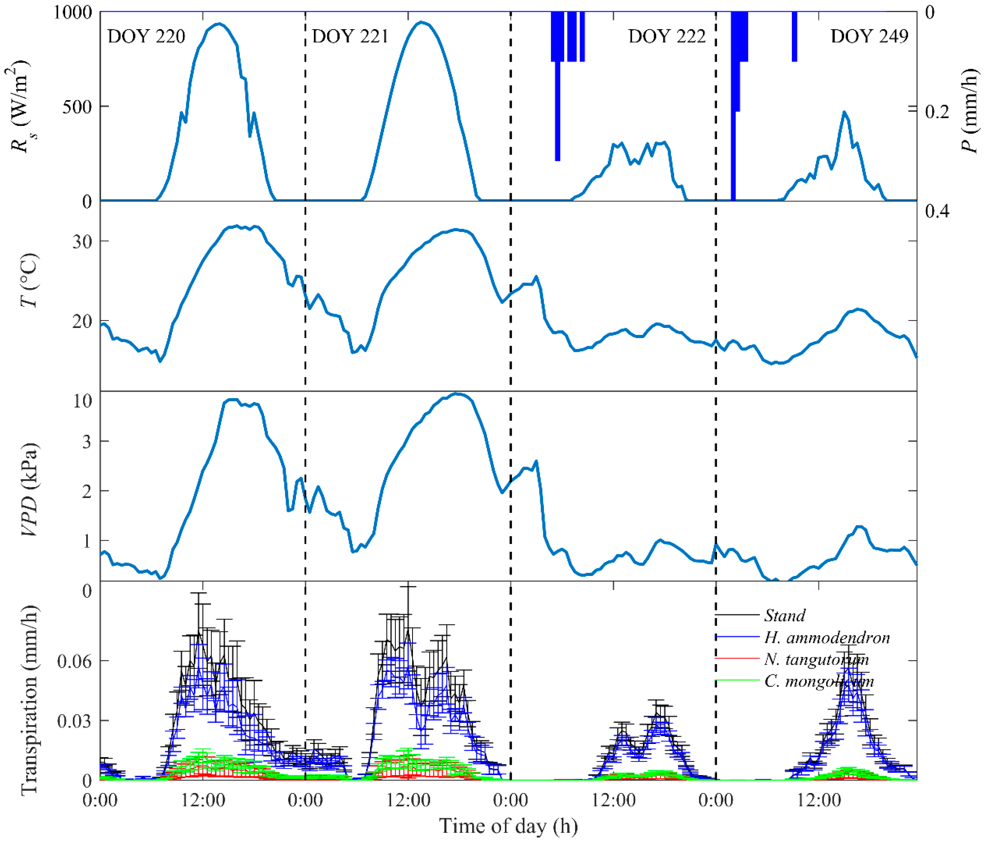
Figure 2 shows the diurnal variations of meteorological conditions and transpiration on typical sunny and rainy days. It can be seen that on sunny days, R_s increased rapidly in the early morning (between 6:30 and 8:00), peaked in the noon (between 13:00 and 13:30), then declined and dropped near zero at about 20:30. T increased along with R_s and reached the maximum of 31.9 °C between 3:30 and 4:00. VPD varied synchronously with T, which rapidly increased in the morning and reached the maximum of 3.8 kPa between 3:30 and 4:00. Stand transpiration increased rapidly in the early morning, peaked at about 11:00, gradually declined throughout the afternoon, and reached the minimum after midnight. For individual species, transpiration in H. ammodendron resembled the temporal pattern of the stand as this species contributed to the largest proportion of the stand transpiration. The maximum transpiration in N. tangutorum and C. mongolicum occurred later at about 12:00. On rainy days, both stand- and species-specific transpiration considerably decreased due to the decrease in atmospheric evaporative demand represented by lower R_s, T, and VPD. On both sunny and rainy days, hourly stand transpiration was closely related to changes in three environmental variables. We observed a notable midday depression of transpiration during the examined period, which was also reported by other studies in arid and semi-arid habitats [33,34]. The depression is mainly caused by stomata closure in response to high vapor-pressure deficit and irradiance in the midday in water-limited ecosystems [34,35]. During the measuring period, the maximum stand transpiration ranged from 0.009 ± 0.003 to 0.10 ± 0.02 mm/h in 2014 and ranged from 0.006 ± 0.002 to 0.12 ± 0.01 mm/h in 2015.

3.3. Control of Environment Variables on Stand Transpiration

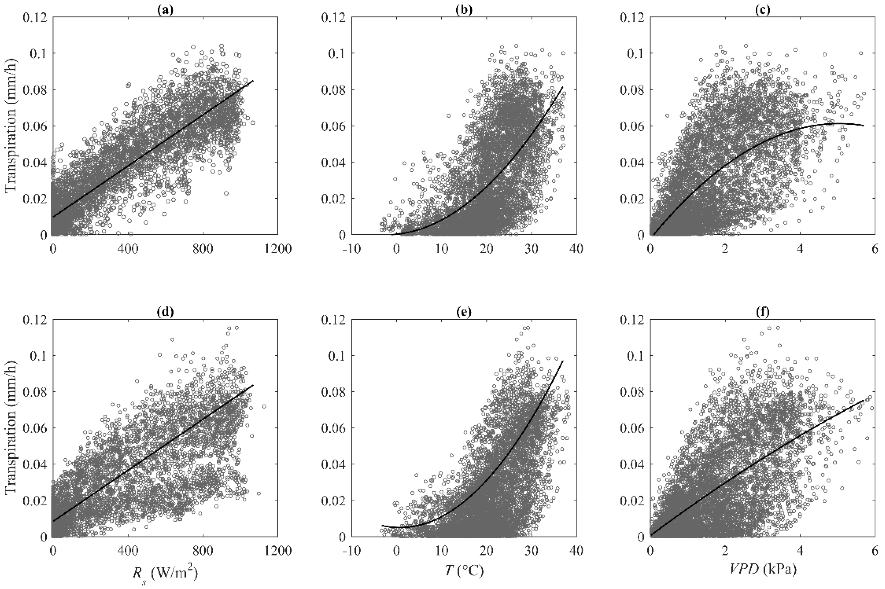
Relationships between hourly stand transpiration and three key environmental variables, namely, hourly R_s, T and VPD, during two-year periods are scatter-plotted in Figure 3. Stand transpiration had a linear correlation with R_s (R² = 0.81 in 2014, 0.64 in 2015). Relationships between stand transpiration and T and VPD were well fitted by a two-degree polynomial function (R² = 0.41 in 2014, 0.42 in 2015 for T; R² = 0.44 in 2014, 0.40 in 2015 for VPD). The general patterns between transpiration and three environmental variables are different from water-unlimited ecosystems [3,36,37]. For example, Wang et al. [3] examined relationships between hourly transpiration and VPD in the Scots pine (Pinus sylvestris) and found that an increase in VPD resulted in a linear increase in transpiration. We performed stepwise regression to reveal how the environmental variables interactively control stand transpiration. The determination coefficients (R²) of the regression analysis and specific equation are given in

Table 4. Determination coefficient (R²) of the seasonal bivariate and trivariate stepwise regression models in which stand transpiration is the dependent variable and solar radiation (R_s), air temperature (T), and vapor pressure deficit (VPD) are independent variables.

Year	Variable	All-time	Jun	July	August	September	October
2014	Rs, T, VPD	0.84	0.87	0.83	0.84	0.88	0.80
	Rs, T	0.84	0.87	0.83	0.84	0.88	0.79
	Rs, VPD	0.84	0.87	0.83	0.84	0.88	0.79
	T, VPD	0.43	0.49	0.41	0.43	0.43	0.79
2015	Rs, T, VPD	0.77	0.87	0.84	0.84	0.88	0.80
	Rs, T	0.76	0.87	0.83	0.84	0.88	0.79
	Rs, VPD	0.76	0.87	0.83	0.84	0.88	0.79
	T, VPD	0.43	0.49	0.41	0.43	0.43	0.40

and

Table A1. Multivariate linear equation between stand transpiration (E_t) and solar radiation (R_s), air temperature (T), and vapor pressure deficit (VPD).

Time		Rs, T & VPD	Rs & T	Rs & VPD	T & VPD
2014	all-time	Et = 0.001 + 0.0001Rs + 0.0003T + 0.004VPD	Et = −0.003 + 0.0001Rs + 0.0007T	Et = −0.003 + 0.0001Rs + 0.004VPD	Et = −0.004 + 0.0008T + 0.011VPD
	Jun	Et = −0.002 + 0.0001Rs + 0.0004T + 0.005VPD	Et = −0.014 + 0.0001Rs + 0.0014T	Et = −0.014 + 0.0001Rs + 0.005VPD	Et = −0.022 + 0.002T + 0.006VPD
	July	Et = 0.007 + 0.0001Rs − 0.0002T + 0.005VPD	Et = −0.009 + 0.0001Rs + 0.001T	Et = −0.009 + 0.0001Rs + 0.005VPD	Et = −0.033 + 0.0025T + 0.004VPD
	August	Et = −0.003 + 0.0001Rs + 0.0006T + 0.001VPD	Et = −0.007 + 0.0001Rs + 0.001T	Et = −0.007 + 0.0001Rs +0.001 VPD	Et = −0.041 + 0.0033 T − 0.002 VPD
	September	Et = −0.004 + 0.0001Rs +0.0008T + 0.001VPD	Et = −0.005 + 0.0001Rs + 0.0009T	Et = −0.005 + 0.001Rs + 0.001 VPD	Et = −0.022 + 0.0001T + 0.003VPD
	October	Et = 0.002 + 0.0001Rs +0.0005T + 0.003VPD	Et = 0.002 + 0.0001Rs + 0.0002T	Et = 0.002 + 0.0001Rs + 0.001 VPD	Et = 0.001 + 0.001T + 0.005VPD
2015	all-time	Et = −0.009 + 0.0001Rs +0.0007T + 0.003VPD	Et = −0.012 + 0.0001Rs + 0.001T	Et = −0.012 + 0.0001Rs + 0.003VPD	Et = −0.009 + 0.001T + 0.009VPD
	Jun	Et = −0.002 + 0.0001Rs +0.0004T + 0.005VPD	Et = −0.014 + 0.0001Rs + 0.0014T	Et = −0.014 + 0.0001Rs + 0.005VPD	Et = −0.022 + 0.0021T + 0.006VPD
	July	Et = 0.007 + 0.0001Rs − 0.0002T + 0.005VPD	Et = −0.009 + 0.0001Rs + 0.0009T	Et = −0.009 + 0.0001Rs + 0.005VPD	Et = −0.033 + 0.0024T + 0.004VPD
	August	Et = −0.003 + 0.0001Rs +0.0006T + 0.001VPD	Et = −0.007 + 0.0001Rs + 0.0009T	Et = −0.007 + 0.0001Rs + 0.001VPD	Et = −0.041 + 0.0033T − 0.002VPD
	September	Et = −0.004 + 0.0001Rs +0.0008T + 0.001VPD	Et = −0.005 + 0.0001Rs + 0.0009T	Et = −0.004 + 0.0001Rs + 0.001VPD	Et = −0.022 + 0.0025T − 0.003VPD
	October	Et = 0.002 + 0.0001Rs +0.0002T + 0.003VPD	Et =0.002 + 0.0001Rs + 0.0005T	Et = 0.002 + 0.0001Rs + 0.003VPD	Et = 0.001 + 0.001T − 0.005VPD

, respectively. Three variables together explained 84% of the variance in stand transpiration in 2014, and explained 77% of the variance in 2015. R² was significantly decreased when R_s was not considered, suggesting that stand transpiration was primarily controlled by energy availability. The regression analysis for each month showed similar results.

Analyzing the relationship between stand transpiration and VPD, we found that stand transpiration increased rapidly with an increase in VPD while it decreased with VPD > 2 kPa. The threshold control of VPD (~2 kPa) on stand transpiration in the two-year examined period suggests a stomata regulation of transpiration [38,39]. The result is generally consistent with the studies by Zheng et al. [11], Bai et al. [14], and Tie et al. [40], although with a somewhat different VPD threshold. However, Shen et al. [13] found that the sap flow density of shelter-belt trees in an arid inland river-basin increased logarithmically with VPD. Du et al. [41] reported that the sap flow density of the three forest species growing in the semiarid Loess Plateau region of China saturated at high VPD. These results suggested that relations between transpiration and VPD are not only climate specific but also ecosystem specific.

Relations between stand transpiration and soil moisture were weak. The correlation coefficient between stand transpiration and surface soil moisture was 0.05 in 2014 and −0.12 in 2015; the corresponding value for the whole layer soil moisture (0−120 cm) was 0.11 in 2014 and 0.19 in 2015. This finding is in line with Du et al. [41]. They analyzed the effects of soil moisture on three native and exotic species living in a semi-arid habitat and found that the sap flow density in native species was less sensitive to changes in soil water conditions. However, our result was different from Bovard et al. [5], who observed that hourly sap flow in three forest species declined in dry soil when VPD was higher than 1 kPa and Yin et al. [42] who reported that cumulative sap flow of the Salix matsudana living in semi-arid Hailiutu River catchment was significantly and negatively correlated with soil water content. This is mainly because the H. ammodendron community is dominated by drought-resistant shrub species which adopted a more conservative water use strategy for preventing excessive water loss during long-period drought [19,41].

3.4. Hysteresis between Stand Transpiration and Environmental Variables

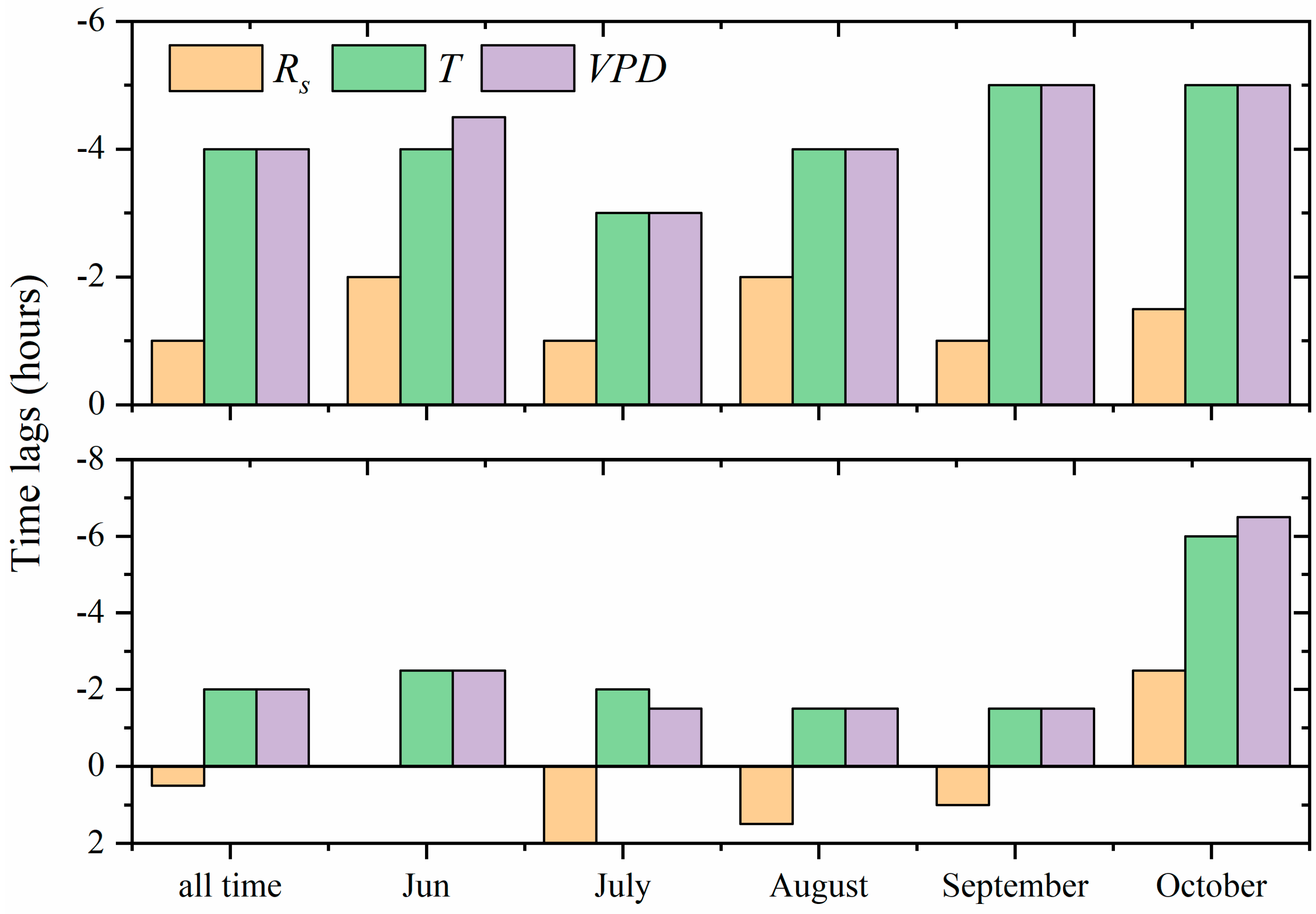
To further elucidate relationships between transpiration of the H. ammodendron shrubland and related environmental factors, we examined time lags between diurnal maximum transpiration and three key environmental variables during the two-year periods. During the growing season in 2014, the average time of maximum transpiration, R_s, T, and VPD were 12:00 pm, 13:30 pm, 4:30 pm, and 4:30 pm, respectively. The corresponding times in 2015 were 14:30 pm, 14:00 pm, 4:30 pm, and 4:30 pm, respectively. In 2014, the mean time lags between maximum diurnal transpiration and three variables were 1.5, 4.5, and 4.5 h, respectively, with transpiration occurring before all environmental maxima. Maximum transpiration occurred after maximum R_s for half an hour but before the maximum T and VPD for two hours in 2015. We further examined the seasonality of the time lags and found that it varied among months (Figure 4b). For T and VPD, time lags decreased from the beginning of the growing season until mid-growing season (July in 2014, August in 2015) and then began to increase towards the end of the growing season. The longest time lags between transpiration and VPD (or T) occurred in October, whereas the shortest time lags were in July. Time lags between transpiration and R_s had less seasonal regularity compared to time lags between transpiration and VPD and T in the two study years. Wang et al. [3] and Zheng et al. [43] also observed seasonality of time lags in their study. The driving force, however, is still unclear.

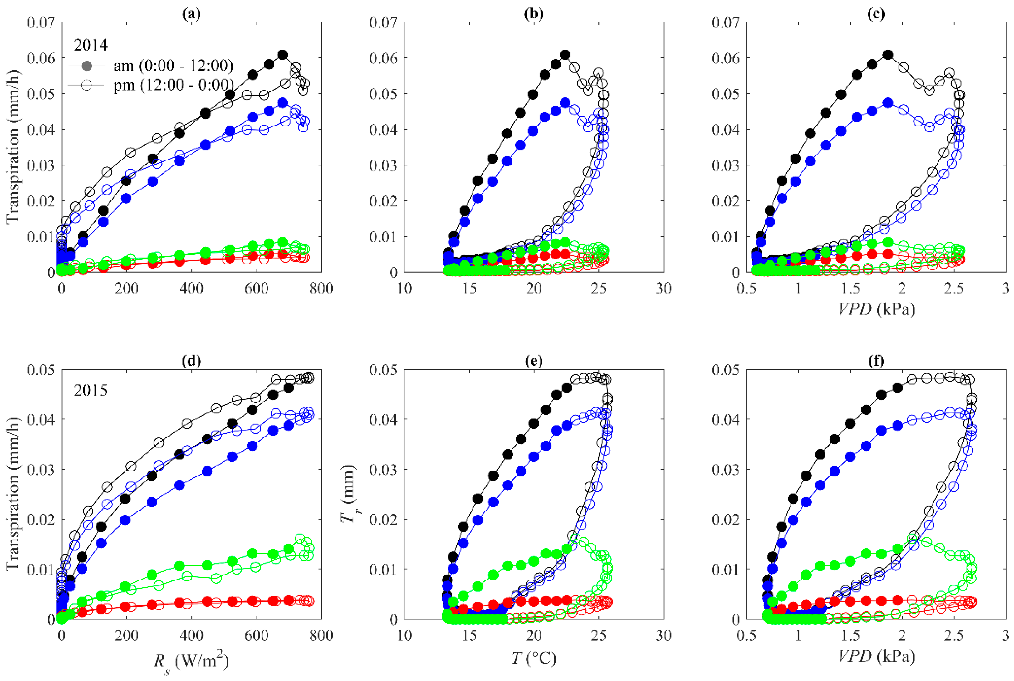
Plots of 30-min average stand transpiration against R_s, T, and VPD revealed clockwise hysteresis loops for T and VPD in the two-year examined periods, whereas hysteresis was eliminated or considerably reduced in the R_s plots (Figure 5). These patterns are consistent with all three species. The clockwise hysteresis loops between transpiration and T and VPD were in line with previous studies such as Tie et al., O’Grady et al., and Matheny et al. [40,44,45]. However, the result is contrary to Wang et al.’s [3] finding in Scots pine (Pinus sylvestris), where dominant anti-clockwise loops were observed for T and VPD. This is mainly because frequent precipitation during their examined period could reduce limitation of water availability and allow transpiration evaporative demand to be relatively constant. Plants tend to close stomatal aperture in the afternoon under high evaporative demand to avoid excessive water loss and thus inhibit transpiration [14,18,36,44,46].

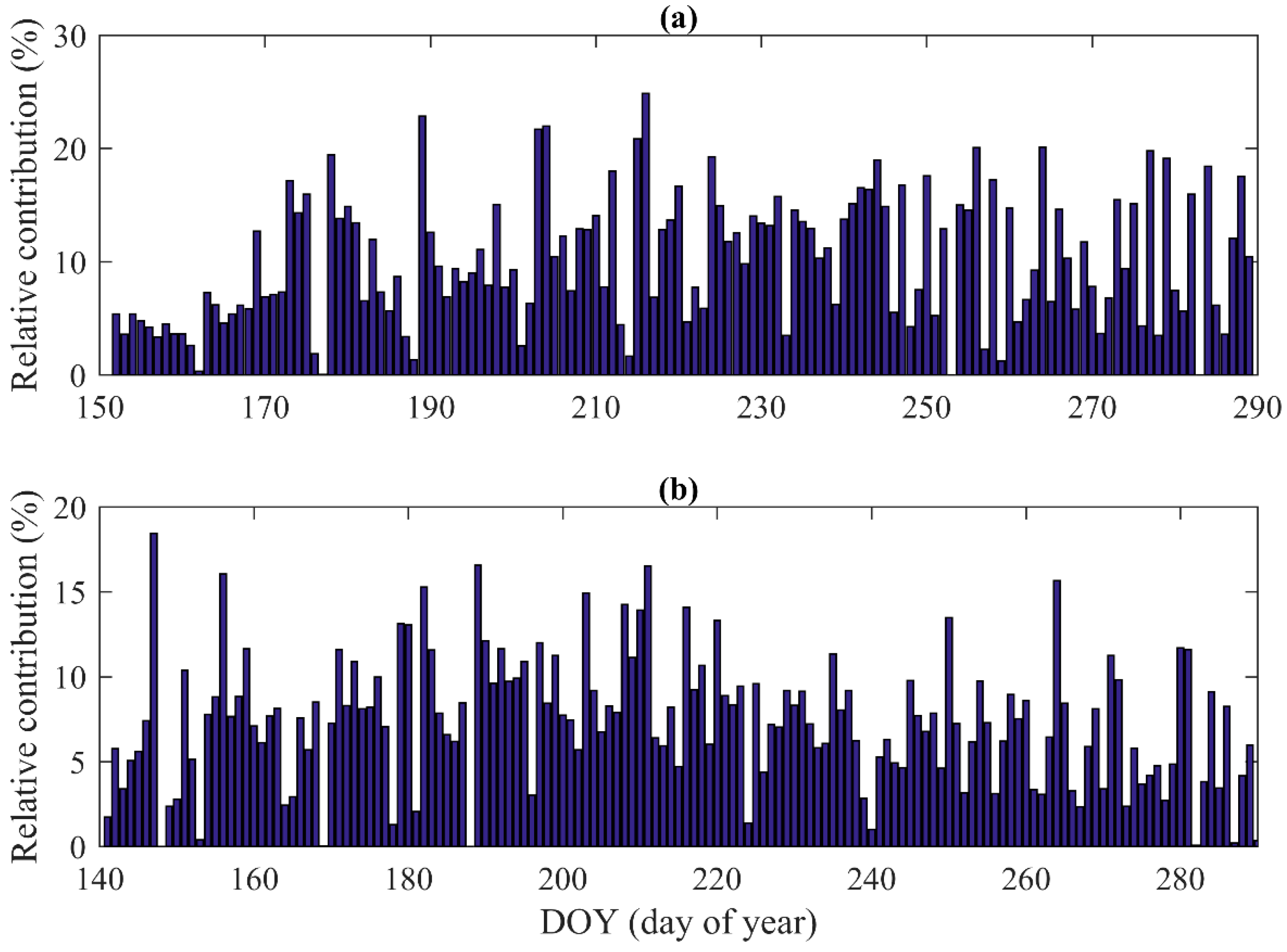
Another possible reason for the hysteresis may be regulation of the water storage in the stems of the shrub, with the release of storage water as sap flow in the early morning prior to variations of the atmosphere conditions [47,48]. We quantified nocturnal sap flow (defined as PAR equals to zero [39] ) to daily total water use and found that the contribution of nocturnal sap flow to daily total water use ranged from 0.01% to 25% with a mean value of 10% in 2014, and ranged from 0.02% to 34% with a mean value of 8% in 2015 (Figure 6). We also observed that nocturnal sap flow was more prominent before midnight, indicating that sap flow before midnight may be used for replenishing the water lost by daytime transpiration (Figure 2). The problem that attributes the nocturnal sap flow to stem water storage is that nighttime sap flow is possibly used for nighttime transpiration [49,50,51]. We found that VPD and u, the factors that usually driving nighttime transpiration [52,53,54], together explained 44% and 41% variations of the nighttime sap flow in 2014 and 2015, respectively (

Table 5. Multivariate linear equation between nocturnal sap flow and solar radiation, air temperature and vapor pressure deficit.

Period	Equation	R2
2014	SF = 0.0002 + 0.0137VPD + 0.0040u	0.44
2015	SF = − 0.0012 + 0.013VPD + 0.0026u	0.41

). In summary, both atmospheric drivers and stem water storage are likely causes of the hysteresis.

4. Conclusions

In the current study, we comprehensively investigated environmental control on transpiration of a desert ecosystem within an oasis-desert ecotone. We measured sap flow from three dominant shrub species and concurrent environmental variables during the growing season in 2014 and 2015. The PCA analysis showed that atmospheric evaporative demand explained the largest proportion of the variance in the environmental data, followed by soil and precipitation indexes. We observed notable midday depression of transpiration during the examined period. At the hourly scale, variations in stand transpiration were closely related to changes in R_s, T, and VPD. Three factors together explained 84% and 77% variations in stand transpiration in 2014 and 2015, respectively, with R_s being the primary driving force. We observed a threshold control of VPD (~2 kPa) on stand transpiration in the two-year examined periods, which was different from patterns of water-unlimited ecosystem and a part of a water-limited ecosystem. The result suggest a strong stomata regulation of transpiration of the selected desert ecosystem under high evaporative demand conditions. Stand transpiration was not sensitive to changes in soil moisture, as the studied ecosystem was dominated by drought-resistant species which adopt a more conservative water use strategy for preventing excessive water loss during long-period drought. Clockwise hysteresis loops between hourly transpiration and T and VPD were observed during the two growing seasons and exhibited seasonal variations. Both the time lags and stem water storage were possible causes of the hysteresis, while more sophisticated field experiments are required to separate their individual contributions. Our work provides insights into environmental controls on the water flux of arid and semi-arid regions at ecosystem scale and implications for diurnal hydrology modeling, in particular on diurnal transpiration and water stress modeling.

References

- Beuhler, M. Potential impacts of global warming on water resources in southern California. Water Sci. Technol. 2003, 47, 165–168. [Google Scholar] [CrossRef] [PubMed]
- Wang, K.; Dickinson, R.E. A review of global terrestrial evapotranspiration: Observation, modeling, climatology, and climatic variability. Rev. Geophys. 2012, 50, RG2005. [Google Scholar] [CrossRef]
- Wang, H.; Tetzlaff, D.; Soulsby, C. Hysteretic response of sap flow in Scots pine (Pinus sylvestris) to meteorological forcing in a humid low-energy headwater catchment. Ecohydrology 2019, 12, e2125. [Google Scholar] [CrossRef]
- Smith, D.; Allen, S. Measurement of sap flow in plant stems. J. Exp. Bot. 1996, 47, 1833–1844. [Google Scholar] [CrossRef] [Green Version]
- Bovard, B.D.; Curtis, P.S.; Vogel, C.S.; Su, H.; Schmid, H.P. Environmental controls on sap flow in a northern hardwood forest. Tree Physiol. 2005, 25, 31–38. [Google Scholar] [CrossRef] [Green Version]
- Dalsgaard, L.; Mikkelsen, T.N.; Bastrup-Birk, A. Sap flow for beech (Fagus sylvatica L.) in a natural and a managed forest—effect of spatial heterogeneity. J. Plant Ecol. 2011, 4, 23–35. [Google Scholar] [CrossRef]
- Otieno, D.; Li, Y.; Liu, X.; Zhou, G.; Cheng, J.; Ou, Y.; Liu, S.; Chen, X.; Zhang, Q.; Tang, X. Spatial heterogeneity in stand characteristics alters water use patterns of mountain forests. Agric. For. Meteorol. 2017, 236, 78–86. [Google Scholar] [CrossRef] [Green Version]
- Wilson, K.B.; Hanson, P.J.; Mulholland, P.J.; Baldocchi, D.D.; Wullschleger, S.D. A comparison of methods for determining forest evapotranspiration and its components: Sap-flow, soil water budget, eddy covariance and catchment water balance. Agric. For. Meteorol. 2001, 106, 153–168. [Google Scholar] [CrossRef]
- Zhao, W.; Liu, B.; Chang, X.; Yang, Q.; Yang, Y.; Liu, Z.; Cleverly, J.; Eamus, D. Evapotranspiration partitioning, stomatal conductance, and components of the water balance: A special case of a desert ecosystem in China. J. Hydrol. 2016, 538, 374–386. [Google Scholar] [CrossRef]
- Huang, J.; Zhou, Y.; Yin, L.; Wenninger, J.; Zhang, J.; Hou, G.; Zhang, E.; Uhlenbrook, S. Climatic controls on sap flow dynamics and used water sources of Salix psammophilain a semi-arid environment in northwest China. Environ. Earth Sci. 2015, 73, 289–301. [Google Scholar] [CrossRef]
- Zheng, C.; Wang, Q. Seasonal and annual variation in transpiration of a dominant desert species, Haloxylon ammodendron, in Central Asia up-scaled from sap flow measurement. Ecohydrology 2014, 8, 948–960. [Google Scholar] [CrossRef]
- Ma, J.; Chen, Y.; Li, W.; Huang, X.; Zhu, C.; Ma, X. Sap flow characteristics of four typical species in desert shelter forest and their responses to environmental factors. Environ. Earth Sci. 2012, 67, 151–160. [Google Scholar] [CrossRef]
- Shen, Q.; Gao, G.; Fu, B.; Lv, Y. Sap flow and water use sources of shelter-belt trees in an arid inland river basin of Northwest China. Ecohydrology 2015, 8, 1446–1458. [Google Scholar] [CrossRef]
- Bai, Y.; Zhu, G.; Su, Y.; Zhang, K.; Han, T.; Ma, J.; Wang, W.; Ma, T.; Feng, L. Hysteresis loops between canopy conductance of grapevines and meteorological variables in an oasis ecosystem. Agric. For. Meteorol. 2015, 214, 319–327. [Google Scholar] [CrossRef]
- Zhang, Q.; Stefano, M.; Gabriel, K.; Amilcare, P.; Dawen, Y. The hysteretic evapotranspiration—Vapor pressure deficit relation. J. Geophys. Res. Biogeo. 2014, 119, 125–140. [Google Scholar] [CrossRef]
- Hong, L.; Guo, J.; Liu, Z.; Wang, Y.; Ma, J.; Wang, X.; Zhang, Z. Time-Lag effect between sap flow and environmental factors of Larix principis-rupprechtii Mayr. Forests 2019, 10, 971. [Google Scholar] [CrossRef] [Green Version]
- Bai, Y.; Li, X.; Liu, S.; Wang, P. Modelling diurnal and seasonal hysteresis phenomena of canopy conductance in an oasis forest ecosystem. Agric. For. Meteorol. 2017, 246, 98–110. [Google Scholar] [CrossRef]
- Lin, C.; Gentine, P.; Frankenberg, C.; Zhou, S.; Kennedy, D.; Li, X. Evaluation and mechanism exploration of the diurnal hysteresis of ecosystem fluxes. Agric. For. Meteorol. 2019, 278, 107642. [Google Scholar] [CrossRef]
- Xu, S.; Ji, X.; Jin, B.; Zhang, J. Root distribution of three dominant desert shrubs and their water uptake dynamics. J. Plant Ecol. 2017, 10, 780–790. [Google Scholar] [CrossRef] [Green Version]
- Ji, X.; Kang, E.; Chen, R.; Zhao, W.; Zhang, Z.; Jin, B. The impact of the development of water resources on environment in arid inland river basins of Hexi region, Northwestern China. Environ. Geol. 2006, 50, 793–801. [Google Scholar] [CrossRef]
- Wu, X.; Zheng, X.-J.; Li, Y.; Xu, G. Varying responses of two Haloxylon species to extreme drought and groundwater depth. Environ. Exp. Bot. 2019, 158, 63–72. [Google Scholar] [CrossRef]
- Lü, X.; Gao, H.; Zhang, L.; Wang, Y.; Shao, K. Dynamic responses of Haloxylon ammodendron to various degrees of simulated drought stress. Plant Physiol. Biochem. 2019, 139, 121–131. [Google Scholar] [CrossRef] [PubMed]
- Xu, G.; Yu, D.; Li, Y. Patterns of biomass allocation in Haloxylon persicum woodlands and their understory herbaceous layer along a groundwater depth gradient. For. Ecol. Manag. 2017, 395, 37–47. [Google Scholar] [CrossRef]
- Xu, S.; Yu, Z.; Zhang, K.; Ji, X.; Yang, C.; Sudicky, E.A. Simulating canopy conductance of the Haloxylon ammodendron shrubland in an arid inland river basin of northwest China. Agric. For. Meteorol. 2018, 249, 22–34. [Google Scholar] [CrossRef]
- Allen, R.G.; Pereira, L.S.; Raes, D.; Smith, M. Crop evapotranspiration-Guidelines for computing crop water requirements-FAO Irrigation and drainage paper 56. FAO Rome 1998, 300, D05109. [Google Scholar]
- Baker, J.M.; Van Bavel, C.H.M. Measurement of mass flow of water in the stems of herbaceous plants. Plant Cell Environ. 1987, 10, 777–782. [Google Scholar]
- Dynamax. Dynagage Sap Flow Sensor User Manual. 2009. Available online: http://dynamax.com/images/uploads/papers/Dynagage_Manual.pdf (accessed on 6 April 2013).
- Köstner, B.; Granier, A.; Cermák, J. Sapflow measurements in forest stands: Methods and uncertainties. Ann. For. Sci. 1998, 55, 13–27. [Google Scholar] [CrossRef]
- Hatton, T.J.; Wu, H.I. Scaling theory to extrapolate individual tree water use to stand water use. Hydrol. Process. 1995, 9, 527–540. [Google Scholar] [CrossRef]
- Hatton, T.J.; Moore, S.J.; Reece, P.H. Estimating stand transpiration in a Eucalyptus populnea woodland with the heat pulse method: Measurement errors and sampling strategies. Tree Physiol. 1995, 15, 219–227. [Google Scholar] [CrossRef]
- Allen, S.; Grime, V. Measurements of transpiration from savannah shrubs using sap flow gauges. Agric. For. Meteorol. 1995, 75, 23–41. [Google Scholar] [CrossRef]
- Ford, C.R.; McGuire, M.A.; Mitchell, R.J.; Teskey, R.O. Assessing variation in the radial profile of sap flux density in Pinus species and its effect on daily water use. Tree Physiol. 2004, 24, 241–249. [Google Scholar] [CrossRef] [PubMed] [Green Version]
- Gartner, K.; Nadezhdina, N.; Englisch, M.; Čermak, J.; Leitgeb, E. Sap flow of birch and Norway spruce during the European heat and drought in summer 2003. For. Ecol. Manag. 2009, 258, 590–599. [Google Scholar] [CrossRef] [Green Version]
- Yu, O.; Goudriaan, J.; Wang, T. Modelling diurnal courses of photosynthesis and transpiration of leaves on the basis of stomatal and non-stomatal responses, including photoinhibition. Photosynthetica 2001, 39, 43–51. [Google Scholar] [CrossRef]
- Rodrigues, T.R.; Vourlitis, G.L.; Lobo, F.d.A.; Santanna, F.B.; de Arruda, P.H.; Nogueira, J.d.S. Modeling canopy conductance under contrasting seasonal conditions for a tropical savanna ecosystem of south central Mato Grosso, Brazil. Agric. For. Meteorol. 2016, 218, 218–229. [Google Scholar] [CrossRef] [Green Version]
- Wullschleger, S.D.; Wilson, K.B.; Hanson, P.J. Environmental control of whole-plant transpiration, canopy conductance and estimates of the decoupling coefficient for large red maple trees. Agric. For. Meteorol. 2000, 104, 157–168. [Google Scholar] [CrossRef]
- Clausnitzer, F.; Köstner, B.; Schwärzel, K.; Bernhofer, C. Relationships between canopy transpiration, atmospheric conditions and soil water availability—Analyses of long-term sap-flow measurements in an old Norway spruce forest at the Ore Mountains/Germany. Agric. For. Meteorol. 2011, 151, 1023–1034. [Google Scholar] [CrossRef]
- Meinzer, F.; Goldstein, G.; Holbrook, N.; Jackson, P.; Cavelier, J. Stomatal and environmental control of transpiration in a lowland tropical forest tree. Plant Cell Environ. 1993, 16, 429–436. [Google Scholar] [CrossRef]
- Motzer, T.; Munz, N.; Küppers, M.; Schmitt, D.; Anhuf, D. Stomatal conductance, transpiration and sap flow of tropical montane rain forest trees in the southern Ecuadorian Andes. Tree Physiol. 2005, 25, 1283–1293. [Google Scholar] [CrossRef] [Green Version]
- Tie, Q.; Hu, H.; Tian, F.; Guan, H.; Lin, H. Environmental and physiological controls on sap flow in a subhumid mountainous catchment in North China. Agric. For. Meteorol. 2017, 240, 46–57. [Google Scholar] [CrossRef]
- Du, S.; Wang, Y.; Kume, T.; Zhang, J.; Otsuki, K.; Yamanaka, N.; Liu, G. Sapflow characteristics and climatic responses in three forest species in the semiarid Loess Plateau region of China. Agric. For. Meteorol. 2011, 151, 1–10. [Google Scholar] [CrossRef]
- Yin, L.; Zhou, Y.; Huang, J.; Wenninger, J.; Uhlenbrook, S. Dynamics of willow tree (Salix matsudana) water use and its response to environmental factors in the semi-arid Hailiutu River catchment, Northwest China. Environ. Earth Sci. 2014, 71, 4997–5006. [Google Scholar] [CrossRef]
- Zheng, H.; Wang, Q.; Zhu, X.; Li, Y.; Yu, G. Hysteresis responses of evapotranspiration to meteorological factors at a diel timescale: Patterns and causes. PLoS ONE 2014, 9, e98857. [Google Scholar] [CrossRef] [PubMed]
- O’Grady, A.P.; Worledge, D.; Battaglia, M. Constraints on transpiration of Eucalyptus globulus in southern Tasmania, Australia. Agric. For. Meteorol. 2008, 148, 453–465. [Google Scholar] [CrossRef]
- Matheny, A.M.; Bohrer, G.; Vogel, C.S.; Morin, T.H.; He, L.; Frasson, R.P.d.M.; Mirfenderesgi, G.; Schäfer, K.V.; Gough, C.M.; Ivanov, V.Y. Species-specific transpiration responses to intermediate disturbance in a northern hardwood forest. J. Geophys. Res. Biogeo. 2014, 119, 2292–2311. [Google Scholar] [CrossRef] [Green Version]
- Chen, L.; Zhang, Z.; Li, Z.; Tang, J.; Caldwell, P.; Zhang, W. Biophysical control of whole tree transpiration under an urban environment in Northern China. J. Hydrol. 2011, 402, 388–400. [Google Scholar] [CrossRef]
- Meinzer, F.C.; James, S.A.; Goldstein, G. Dynamics of transpiration, sap flow and use of stored water in tropical forest canopy trees. Tree Physiol. 2004, 24, 901–909. [Google Scholar] [CrossRef] [PubMed] [Green Version]
- Goldstein, G.; Andrade, J.; Meinzer, F.; Holbrook, N.; Cavelier, J.; Jackson, P.; Celis, A. Stem water storage and diurnal patterns of water use in tropical forest canopy trees. Plant Cell Environ. 1998, 21, 397–406. [Google Scholar] [CrossRef]
- Dawson, T.E.; Burgess, S.S.; Tu, K.P.; Oliveira, R.S.; Santiago, L.S.; Fisher, J.B.; Simonin, K.A.; Ambrose, A.R. Nighttime transpiration in woody plants from contrasting ecosystems. Tree Physiol. 2007, 27, 561–575. [Google Scholar] [CrossRef] [Green Version]
- Rosado, B.H.; Oliveira, R.S.; Joly, C.A.; Aidar, M.P.; Burgess, S.S. Diversity in nighttime transpiration behavior of woody species of the Atlantic Rain Forest, Brazil. Agric. For. Meteorol. 2012, 158, 13–20. [Google Scholar] [CrossRef]
- Snyder, K.; Richards, J.; Donovan, L. Night-time conductance in C3 and C4 species: Do plants lose water at night? J. Exp. Bot. 2003, 54, 861–865. [Google Scholar] [CrossRef]
- Daley, M.J.; Phillips, N.G. Interspecific variation in nighttime transpiration and stomatal conductance in a mixed New England deciduous forest. Tree Physiol. 2006, 26, 411–419. [Google Scholar] [CrossRef] [PubMed] [Green Version]
- Phillips, N.; Ryan, M.; Bond, B.; McDowell, N.; Hinckley, T.; Čermák, J. Reliance on stored water increases with tree size in three species in the Pacific Northwest. Tree Physiol. 2003, 23, 237–245. [Google Scholar] [CrossRef] [PubMed] [Green Version]
- Phillips, N.G.; Lewis, J.D.; Logan, B.A.; Tissue, D.T. Inter-and intra-specific variation in nocturnal water transport in Eucalyptus. Tree Physiol. 2010, 30, 586–596. [Google Scholar] [CrossRef] [PubMed] [Green Version]
Figure 1.
Map of the study area (the land-cover types were obtained from the Moderate Resolution Imaging Spectroradiometer (MODIS) 1 km IGBP land cover product.
Figure 2.
Diurnal courses of half-hourly solar radiation (Rs), air temperature (T), vapor pressure deficit (VPD), precipitation (P), and transpiration for typical sunny days (DOY 220 and 221) and rainy days (DOY 222 and 249) in 2014.
Figure 3.
Half hourly stand transpiration against solar radiation (Rs), air temperature (T), and vapor pressure deficit (VPD) during the growing season in (a–c) 2014 and (d–f) 2015.
Figure 4.
Time lags between maximum stand transpiration and environmental variables including solar radiation (Rs), temperature (T), and vapor pressure deficit (VPD) for different months in (a) 2014 and (b) 2015. Positive values indicate that maximum stand transpiration occurred later than maximum environmental variable.
Figure 5.
Hysteresis loops between transpiration (Tr) and solar radiation (Rs), air temperature (T), and vapor pressure deficit (VPD) in (a–c) 2014 and (d–f) 2015. The black, blue, green, and red cycles represent transpiration in the stand, H. ammodendron, N. tangutorum, and C. mongolicum, respectively.
Figure 6.
Relative contribution of nocturnal sap flow to daily total water use during the growing season in (a) 2014 and (b) 2015.