Article

An Evaluation Study of the Fully Coupled WRF/WRF-Hydro Modeling System for Simulation of Storm Events with Different Rainfall Evenness in Space and Time

1
State Key Laboratory of Simulation and Regulation of Water Cycle in River Basin, China Institute of Water Resources and Hydropower Research, Beijing 100038, China
2
College of Hydrology and Water Resources, Hohai University, Nanjing 210098, China
3
Nansen-Zhu International Research Centre, Institute of Atmospheric Physics, Chinese Academy of Sciences, Beijing 100029, China
*
Author to whom correspondence should be addressed.
Water 2020, 12(4), 1209; https://doi.org/10.3390/w12041209
Submission received: 25 February 2020 / Revised: 20 April 2020 / Accepted: 21 April 2020 / Published: 24 April 2020
(This article belongs to the Special Issue Hydrological Modeling in Water Cycle Processes)

Abstract

:
With the aim of improving the understanding of water exchanges in medium-scale catchments of northern China, the spatiotemporal characteristics of rainfall and several key water cycle elements e.g., soil moisture, evapotranspiration and generated runoff, were investigated using a fully coupled atmospheric-hydrologic modeling system by integrating the Weather Research and Forecasting model (WRF) and its terrestrial hydrologic component WRF-Hydro (referred to as the fully coupled WRF/WRF-Hydro). The stand-alone WRF model (referred to as WRF-only) is also used as a comparison with the fully coupled system, which was expected to produce more realistic simulations, especially rainfall, by allowing the redistribution of surface and subsurface water across the land surface. Six storm events were sorted by different spatial and temporal distribution types, and categorical and continuous indices were used to distinguish the applicability in space and time between WRF-only and the fully coupled WRF/WRF-Hydro. The temporal indices showed that the coupled WRF-Hydro could improve the time homogeneous precipitation, but for the time inhomogeneous precipitation, it might produce a larger false alarm than WRF-only, especially for the flash storm that occurred in July, 2012. The spatial indices showed a lower mean bias error in the coupled system, and presented an enhanced simulation of both space homogeneous and inhomogeneous storm events than WRF-only. In comparison with WRF-only, the fully coupled WRF/WRF-Hydro had a closer to the observations particularly in and around the storm centers. The redistributions fluctuation of spatial precipitation in the fully coupled system was highly correlated with soil moisture, and a low initial soil moisture could lead to a large spatial fluctuated range. Generally, the fully coupled system produced slightly less runoff than WRF-only, but more frequent infiltration and larger soil moisture. While terrestrial hydrologic elements differed with relatively small amounts in the average of the two catchments between WRF-only and the fully coupled WRF/WRF-Hydro, the spatial distribution of elements in the water cycle before and after coupling with WRF-Hydro was not consistent. The soil moisture, runoff and precipitation in the fully coupled system had a similar spatial trend, but evapotranspiration did not always display the same.

1. Introduction

Rainfall is an important driver of the water cycle and a key index of the change of weather system [1,2,3]. Additionally, interrelated elements in the water cycle such as runoff, evapotranspiration, and soil moisture also influence water resources, climate, agriculture, and ecosystems in a region [4,5,6]. In recent decades, with the maturity of information collection methodologies such as remote sensing, satellites and communication technology, forecasting through meteorological or climatic patterns has become an effective means for alleviating hazards caused by extreme hydrological events [7,8,9]. The development of climate models [10,11] has effectively linked the atmospheric, surface, and subsurface processes, and prolonged the foreseeing period of storm and flood forecasting. Even so, this is not sufficient to understand and predict how the complex components of the water cycle interact with the complexities of the landscape. First of all, the current atmospheric models mainly apply a relatively simple one-dimensional approach in simulating both the surface and the groundwater processes, while less consideration is given to the lateral interaction among soil, surface and undersurface hydrological features [12,13]. Second, in a standalone hydrological model [14], the output of the climate model is used as the input data to drive the hydrological model, but the indirect connection between the land surface and the atmosphere is neglected [15]. The lack of a feedback mechanism leads to the separation of the atmospheric precipitation and subsequent land surface hydrological processes. At the same time, the lateral water flow generated in the underground interaction and the redistribution of soil moisture cannot be fed back to the atmosphere.
A fully coupled modeling system [16] of the climate model and the hydrologic model is a novel development designed to make up for the aforementioned lack. In the fully coupled system, the climate model is coupled with the hydrologic model through the land surface model (LSM) of the same physical mechanisms, and the input and output of both models provide feedback to each other. The progressive fully coupled modeling system yields regulated topographically-driven soil moisture and land surface fluxes, thus improving the spatiotemporal correlations between the surface and lower atmospheric elements [6]. Maxwell et al. [17] tried to connect the hydrology model ParFlow [18] with the Advanced Regional Prediction System (ARPS) [19] in an idealized experimental simulation. The results showed that the fully coupled system could be used to describe the spatiotemporal correlation between lower atmospheric variables, surface and water table depth. To solve the biochemical shortcomings of the hydrological model, Maxwell et al. [20] introduced Noah LSM to connect ParFlow, and the Weather Research and Forecasting (WRF), tests were still carried out in an idealized experiment scenario and proved that an accurate runoff mechanism and lateral flow could change the spatial distribution of land surface and atmospheric fluxes. Shrestha et al. [8] used the Community Land Model (CLM) to link Parflow with atmospheric model, the Consortium for Small-Scale Modeling (COSMO), to a week prediction in Ruhr basin, Germany. They found the potential of the fully coupled system in surface flux prediction. Gochis et al. [21] proposed a parallel, multicore, multiphysics, multiscale, fully distributed hydraulic model system (WRF-Hydro). WRF-Hydro sets up a multiscale quasi-3D land surface hydrological simulation system to improve the one-dimensional vertical generalization of water transport using the LSM Noah or Noah MP in the WRF model [21]. It could operate independently or be used for the coupling with WRF. WRF-Hydro realizes the effective scale conversion of hydrology and land surface modules, solves the problem of resolution mismatch between a climate model and a hydrologic model [22], and reflects the lateral movement of soil moisture and the interaction between surface water and subsurface water.
The interrelationship promotes the expression of the land surface hydrological process, and the fully coupled WRF/WRF-Hydro is expected to be able to provide feedback and improve the simulations of the WRF model [23,24]. Variables that feedback to each other in the fully coupled WRF/WRF-Hydro include soil moisture, land flues of energy, etc. The coupled WRF/WRF-Hydro system has been applied for studies in a number of places in the world. Senatore et al. [25] conducted a three-year continuous simulation in southern Italy. The results show that the WRF/WRF-Hydro coupling model produced higher soil moisture content and lower overall surface runoff than WRF-only. Xiang et al. [26] investigated the exchange processes between the atmosphere and the land surface using the fully coupled system, by carrying out a comparison experiment from 2004 to 2013 in northwestern Mexico. The results indicated that the soil moisture and vegetation types could affect the convective rainfall, and the initial land surface conditions (such as the soil water storage) were critical for enhancing the simulations. Kerandi et al. [6] explored the simulation with the coupled WRF/WRF-Hydro in a watershed of East Africa from 2011 to 2014, and showed that the precipitation of the coupled system had little variation compared to WRF and might be affected by the moisture advection outside the domain. Both of the above three fully coupled cases focused on the long-term series of simulation. Wehbe et al. [27] gave an analysis of a 3-day extreme event in arid region of United Arab Emirates, and the simulated precipitation suggested reducing root mean square error (RMSE) and relative error (RE) trends in the fully coupled WRF/WRF-Hydro than WRF-only. These previous studies show that atmospheric hydrological coupling models have a significant effect on the simulated atmospheric–terrestrial water balance. However, for the discussion of fully coupled WRF/WRF-Hydro, most of the coupling simulations focus on a long time scale, there were not enough cases and few systematic analyses of storm events with different temporal and spatial consistency and the related changes of water cycle elements in the hydrological processes.
In semi-humid areas of northern China, there is frequent convectional rain and the runoff generation is mixed with infiltration-excess and storage-excess mechanisms. The rain storm events in such areas, featured with high rainfall intensities, pre-dry soil conditions, and inhomogeneous spatiotemporal distributions, need further simulation accuracy of the terrestrial hydrological processes.
This study we explored three basic questions:
  • What are the different spatiotemporal storm simulation performances between WRF-only and the fully coupled WRF/WRF-Hydro in the semi-humid areas of northern China?
  • Could the fully coupled system improve the precipitation spatiotemporal distribution?
  • What are the differences in the variation of water cycle elements (e.g., rainfall and soil moisture) of different storm events?
To answer the problems above, the WRF-only and coupled WRF-Hydro models were applied to two catchments for six 24-hour rainstorm events with different spatiotemporal homogeneousness of the rainfall distribution. The impact of the enhanced description of atmospheric–terrestrial water balance in WRF-Hydro was investigated by comparing WRF-Hydro and WRF-only results with observations over the region. In order to further understand the simulation results, several crucial water cycle elements, i.e., the generated runoff, the evapotranspiration, and the soil moisture were also analyzed and compared between the fully coupled modeling system and the stand-alone WRF model.

2. Data and Methods

2.1. Study Area and Storm Events

The scope of this work covers two basins in the semi-humid regions of northern China: the Fuping catchment with eight rain gauges, and the Zijingguan catchment with eleven rain gauges. Figure 1 shows the gauge locations, DEMs, and WRF nested domains of the two study catchments. The Fuping and Zijingguan catchments, which respectively belong to the south and the north branch of the Daqing river catchment, occupy drainage areas of 2210 and 1760 km2, respectively. The average annual rainfall in the Daqing river catchment was approximately 600 mm. From late May to early September each year, the warm and humid airflow around the tropical low pressure moves towards northern China. The airflow encounters subtropical high pressure and the Taihang Mountain topography to stop its movement and gradually slow down. There is weak cold air activity in the study areas, and cold and warm air interact with local strong convective rainfall.
For the classification of the storm events, the temporal and spatial homogeneousness of the rainfall occurring in the two basins was analyzed by calculating the storm events coefficient of variance (Cv), since the lower the Cv value, the more homogeneous the rainfall [28]. Cv can be written as follows:
C v = i = 1 N ( x i x ¯ 1 ) 2 N
where x ¯ is the average of xi. When the calculation is for the spatial distribution, the spatial Cv value calculated by Equation (1) means the variability of the spatial rainfall distribution, xi is the 24 h rainfall accumulation of the ith station, and N is the number of rain gauges, hence the spatial Cv reflects an average of the cumulative deviation of all time steps at each rain gauge; when the calculation is for the time distribution, the temporal Cv means the variability of the temporal rainfall distribution, xi is the catchment average rainfall of the ith-hour, and N is the total number of hours for the storm duration. At this time, the temporal Cv value represents an average of the cumulative deviation of all rain gauges in each time step.
Unlike the southern regions of China, it is difficult to find truly homogeneous rainfall in northern China. The spatial Cv and temporal Cv of precipitation events that occurred in the two basins from 1985 to 2015 were separately sorted according to frequency. For both spatial Cv and temporal Cv, there was a critical value of 5% frequency, which was taken as a Cv threshold value to separate homogeneous and inhomogeneous storm events [29]. That is to say, the temporal or spatial homogeneousness was determined when the Cv values of storm events were less than the threshold Cv values, which were 0.4 in time and 1.0 in space, respectively.
Six typical and representative events in the two basins from 2005 to 2015 were selected for simulation and the detail rainfall information on the events and the judgment of the rainfall type are shown in Table 1, wherein the rainfall distribution of Type 1 (including Event 1) was homogeneous in both space and time, Type 2 (including Event 2) was homogeneous in space but inhomogeneous in time, and Type 3 (including the other four events) was inhomogeneous in both space and time. It should be pointed out that the soil moisture levels in Event 4 and Event 6 were relatively dry before raining, and Event 5 had the shortest rainfall duration and the largest accumulative rainfall of six storm events. There is a 24 h statistical window, which can completely cover the precipitation process of the selected storm events.

2.2. Models and Calibration

2.2.1. WRF

The Weather Research and Forecasting (WRF) model, which based on the mesoscale atmospheric model (MM5), was designed as a new generation of numerical weather prediction (NWP) to be applied for a wide range of research and operational prediction problems. [30,31,32,33]. In this study, three nesting domain are set up for WRF (Figure 1): the innermost Dom3 has 1 km pixel size, the second Dom2 has 3 km pixel size, and the outer Dom1 has 9 km pixel size. The driving data were acquired from the Final Operational Global Analysis (FNL) data of the National Centers for Environmental Prediction (NCEP) to provide WRF with initial and boundary fields. The different options for physical parameterization schemes need attention in different practical applications. In this study, based on the climatic characteristics and the underlying conditions of the two study catchments, the Yonsei University of microphysical processes scheme [34], the Kain–Fritsch of boundary layer scheme [35] and the Purdue–Lin of cumulus convection scheme [36] were screened. It should be noted that the cumulus convection scheme was not used in the innermost Dom3 where the convective rainfall generation is assumed to be explicitly resolved [37]. Table 2 lists the experimental details and physics schemes of the WRF related configurations.

2.2.2. WRF-Hydro

The WRF-Hydro model used in this study was version 3.0 [38,39], and the information about the WRF-Hydro model is available on the official website [40]. WRF-Hydro mainly includes a LSM module, a hydrologic module and a disaggregation–aggregation module.
1. Runoff generation in Noah
The LSM coupled with WRF/WRF-Hydro are Noah in this case [38,39]. There are four soil layers in a 2-meter soil column used in Noah, and the soil column configuration used in this study had the depth of the bottom of the layers as 0–10cm, 10–40cm, 40–100cm, and 100–200 cm. The runoff generation process in Noah is divided into three parts: surface excess infiltration runoff, saturated subsurface runoff and deep underground free outflow. The process of excess infiltration runoff generation is the simple water balance (SWB), derived by Schaake et al. [41], which follows the assumption that when the infiltration is greater than the grid surface aquatic water capacity (precipitation reduced by the interception and evaporation), the excess part of infiltration produces surface runoff. Then, with the increase of infiltration, the subsurface water in each layer of soil column gradually accumulates. The subsurface water occurs until the existing soil water content soil moisture exceeds the total saturated soil moisture of the whole soil column. There is also a water outlet at the bottom of each grid soil column, which is used to indicate a deep free drainage process.
2. Routing in the hydrological module
The hydrological module of WRF-Hydro compensates and strengthens the description of the lateral transport of the infiltration excess process and of the saturated subsurface process in Noah. Corresponding to runoff generation, it includes overland routing, subsurface routing, deep base flow, and a river routing. The overland routing is realized similar to Downer et al. [42] by a completely unsteady, finite difference and diffusion wave method. The flow on the reverse slope and backwater effects are taken into account in the diffusion wave equation. The subsurface routing refers to the saturated flow in the soil layer, and its lateral movement is according to the method proposed by Wigmosta and Lettenmaier [43], where a quasi-three-dimensional flow is computed, including the effects of topography, saturated soil depth and saturated hydraulic conductivity varying with soil depth. Channel routing, similar to overland flow, uses an explicit, one-dimensional, variable time step diffusion wave equation. When the water depth of the grid column exceeds a predefined retention depth, the stream inflow occurs and gradually flows along the channel grids. The base flow is represented by a simple, experience-based bucket model located below the soil column and is the construction of a conceptual bucket model with side openings, which is especially suitable for a long-term simulation. An exponential function is used to achieve the conceptual water depth in the bucket, and the water discharged from the soil column is mapped to the underground bucket according to a scale factor. The water in the bucket is gradually returned to the channel section directly corresponding to its downstream catchment area. The current hydrological module of WRF-Hydro does not support the coupling of river channel and base flow.
3. Configurations of WRF-Hydro and disaggregation–aggregation module
The configurations related to the WRF-Hydro are shown in Table 3. The base flow module is closed in this study for a short simulation time and it simply collects underground runoff and reallocates it to the channel, which can easily provide additional river flow [19]. The fully coupled method is realized by recompiling and merging WRF-Hydro into WRF. As the carrier of linking WRF and hydrological modules, LSM realizes the complete interaction of model state variables and flux variables by calling the disaggregation–aggregation module. The Noah in WRF-Hydro requires forcing data including precipitation, 2m surface temperature, surface pressure, long and short wave radiation, and leaf area index. When the fully coupled option is turned on, running WRF will call the LSM module, disaggregation–aggregation module and hydrological module components of WRF-Hydro. Runoff generated in Noah before the grid disaggregation process is "on", and the proportion of downscaling factor is 10. This means that the variables of Noah (the maximum soil moisture content and lateral saturated hydrological conductivity of different soil type, the excess infiltration, the soil water content of each soil layer, etc.,) generated by each 1km × 1km grid are disaggregated into 100m × 100m subgrids by assigning linear weighting factors for subsurface and overland routing. Then, through a linear average of the subgrids, the fine grid variables generated by overland routing (water accumulation depth) and subsurface routing (soil moisture content of each soil layer) of the hydrological module are aggregated back to the Noah grid and the updated soil moisture and heat flux are fed back to WRF for the next iterative cycle. For details of the grid disaggregation–aggregation process, refer to the description of Gochis and Chen [44].

2.2.3. WRF-Hydro Calibration

Before analyzing the influence of WRF and the fully coupled WRF/WRF-Hydro, we calibrated the stand-alone WRF-Hydro parameters, and then selected the same parameter group in the coupled system. It should be pointed out that the stand-alone WRF-Hydro forcing input time step must be consistent with the WRF model output time step (1 h) for it was a necessary compilation rule for guaranteeing the data generated by WRF can be used to drive WRF-Hydro.
Four parameters were used for the calibration and sensitivity analysis, including the runoff infiltration parameter (REFKDT), the surface retention depth scaling parameter (RETDEPRTFAC), the overland flow roughness scaling parameter (OVROUGHRTFAC) and the channel Manning roughness (MannN). REFKDT is a significant parameter for the infiltration excess process. RETDEPRTFAC should be adjusted depends on the surface slope, and in general, in regions where slopes are steeper than 30°–45°, and there is no accumulation or retention. Increasing REFKDT and RETDEPRTFAC affect the total water volume by encouraging more local infiltration near the river channel to wetter soils and thus, to better riparian conditions. OVROUGHRTFAC depends on the land-use type, and also influences the amount of water that is transferred to the channel grids. It also has an impact on the hydrograph shape, but OVROUGHRTFAC in controlling the speed of the overland transmitters downstream and the amount of water on a column scale is relatively minimal. Instead, MannN has obvious impact on the streamflow to channel grids. Decreasing MannN and OVROUGHRTFAC accelerated the routing of the river channel, resulting in a higher flood peak [45,46]. This is also supported by the conclusions from other studies (e.g., Kerandi et al. [6], Senatore et al. [25], Naabil et al. [45] and Ryu et al. [46]). To minimize model runs and cut down computational time, the calibration process used a stepwise approach [47] which denotes that the determination of one parameter will be verified before the next parameter is calibrated. This approach made it possible to adjust the model to best fit the observations of streamflow and timing. We mainly calibrated order is REFKDT, MannN, RETDEPRTFAC and OVROUGHRTFAC. Aside from the four main parameters, the other parameters are set to their defaults, owing to the lack of observational data.

2.3. Evaluation Statistics

Both the 24 h accumulation and the spatiotemporal distributions of rainfall are evaluated for WRF-only and the fully coupled WRF/WRF-Hydro modeling system. While calculating average rainfall, the relative error (RE) was first evaluated:
RE = | P s P o P o | × 100 % ,
where Ps and Po are the simulated and observed 24 h cumulative rainfall values in the two study areas calculated based on rain gauges [48].
For the evaluation indices of the spatial and temporal rainfall distributions, five indices which refer to [28] are used, i.e., the critical success index (CSI), the probability of detection (POD), the false alarm ratio (FAR), the root mean square error (RMSE), and the mean bias error (MBE). The meanings of the above indices and the range values are provided in Table 4. Among these indices, FAR, CSI, and POD are categorical, and RMSE and MBE are continuous indices [49,50].
The categorical indices were as follows:
POD = 1 N i = 1 N N A i N A i + N C i ,
FAR = 1 N i = 1 N N B i N A i + N B i ,
CSI = 1 N i = 1 N N A i N A i + N B i + N C i ,
The calculation of categorical indices is based on a rain/no rain contingency table, as shown in Table 5. The NA, NB, NC, and ND represent the total hit numbers of the eligible judgment, whether the simulated and observed values in an observation period or at the observation position were greater than 0.01 mm (judgment of whether rainfall occurred) and NA = i = 1 N N A i , NB = i = 1 N N B i , N C = i = 1 N N C i , ND = i = 1 N N D i . When evaluating on a temporal dimension, the rainfall simulations and observations of different time steps were compared at the same rainfall gauges i, and N referred to the number of the rain gauges. When evaluating on a spatial dimension, the rainfall simulations and observations of the different rain gauges were compared with the same hourly time step i, and N (N = 24) referred to the number of time steps.
There is a general evaluation of simulated performance on the basis of the correctness of rainfall occurrences in categorical indices, and continuous indices are provided for a more quantitative calculation of the simulated error.
The continuous indices were calculated as follows:
RMSE = 1 M j = 1 M ( P s j P o j ) 2 ,
M B E = 1 M j = 1 M ( P s j P o j ) ,
When the indices were calculated in the temporal dimension, M (M = 24) was the number of time steps, and Psj and Poj were the simulated and observed average areal rainfall of the study catchment at each time step j. When the indices were calculated in the spatial dimension, M was the total number of each rain gauges, which is 8 for the Fuping catchment and 11 for the Zijingguan catchment and Psj and Poj were the simulated and observed values of accumulated rainfall at each rain gauge j. Both MBE and RMSE represent an average cumulative error, but in MBE, the error including the direction, might induce gradually random errors canceled out during a rainfall period.

3. Results and Discussions

The presentation is divided into two parts: the first part is the analysis of different types of rainfall in time and space between WRF-only and the fully coupled WRF/WRF-Hydro system according to RE, five spatiotemporal indices and the spatial distribution map of 24 hours accumulative rainfall; the second part is the temporal and spatial changes between soil moisture, runoff and evapotranspiration in the water cycle and their relationship with different types of rainfall.

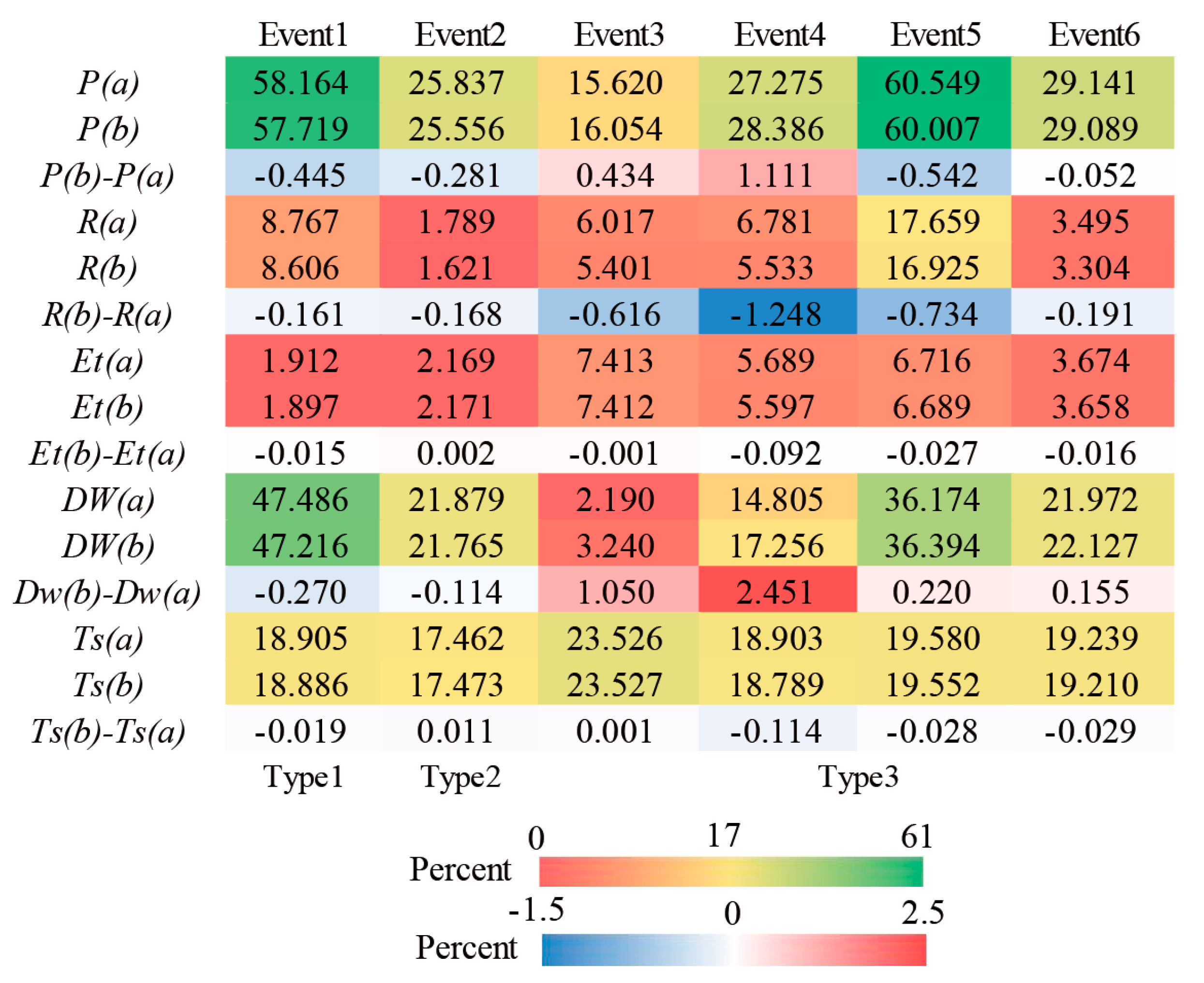
3.1. Rainfall Simulations by WRF-Only and the Fully Coupled WRF/WRF-Hydro

3.1.1. The 24 h Accumulation of Rainfall

Figure 2 shows the 24 h rainfall histogram and cumulative curve. For both WRF-only and the fully coupled WRF/WRF-Hydro, the RE was truly related with the temporal and spatial homogeneousness of storm events. It could be grasped intuitively that the cumulative rainfall of the coupled system was generally closer to the observations than that of WRF-only, except Event 5. Table 6 further provides the relative error (RE), different type rainfall average relative error (ARE) of the 24 h cumulative rainfall curve and 24 h rainfall accumulation values using WRF-only simulation and the fully coupled WRF/WRF-Hydro simulation. For the three types of events, the values of ARE (b) were all less than ARE (a), which might mean that the fully coupled WRF-Hydro could improve the cumulative rainfall compared with WRF-only. The results of ARE values were type 3>type 2>type 1, which were reasonable for the inhomogeneous spatial and temporal distribution, led to worse simulations. The RE of Event 1–4 of the fully coupled modeling system were less than WRF-only. In particular, the Event 1 simulated and observed RE was reduced from 0.139 (WRF-only) to 0.038 (the fully coupled WRF/WRF-Hydro). Nevertheless, the fully coupled system cumulative rainfall values of Event 5, an extreme heavy storm mentioned before, were slightly less, with the associated RE values that rose from 0.657 (the fully coupled WRF/WRF-Hydro) to 0.616 (WRF-only).

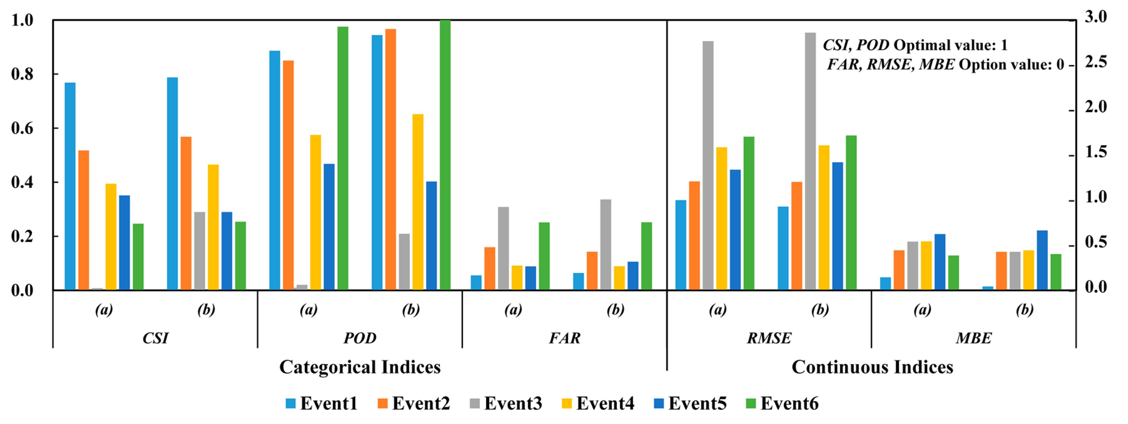
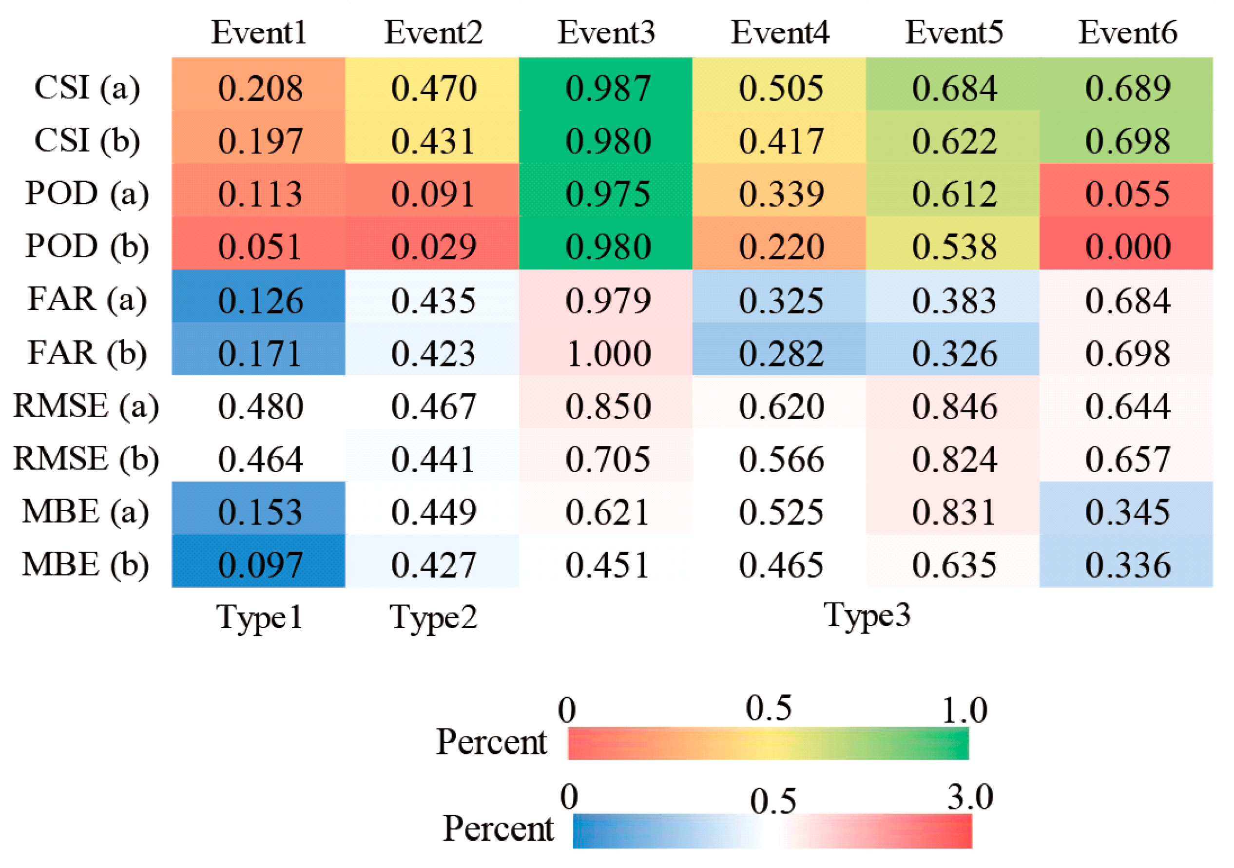
3.1.2. Indices for the Temporal Rainfall Distribution

Figure 3 is the temporal results of the five indices for WRF-only and the fully coupled WRF/WRF-Hydro model. For both the fully coupled WRF/WRF-Hydro and WRF-only, it could be determined that the temporal indices results were Type 1>Type 2>Type 3, from the best to the worst. For events in Type 3, the RMSE values in the fully coupled WRF-Hydro were all higher than WRF-only, which might mean a more accumulative error without canceling out the positive and negative errors in time inhomogeneous events.
We further calculated the difference between each index value and its optimal value as the indices errors. That is, for CSI and POD, the indices errors were the positive difference between the corresponding indices and 1; for FAR, RMSE and MBE, and the indices errors were the positive difference with 0.The temporal heat map is shown in Figure 4. Lower indices errors compared with WRF-only indicated that the fully coupled WRF-Hydro improved time distribution of Type1 and Type 2 events. However, in Type 3, Event 3 and Event 6 have the largest (2.393) and second largest (1.887) temporal Cv values, which might mean a more uneven time distribution in Type 3. In both the fully coupled WRF-Hydro and WRF-only, the CSI, FAR and POD errors for Event 3 were the largest, which meant a worse rainfall occurrences simulation in time. Consistent with this, the RMSE error for Event 3 was the highest, but the decreasing MBE error represented the real random errors canceled out of the total rainfall amount. The indices of Event 6 showed a similar trend with a second worst CSI, FAR and RMSE, but a second best MBE.
The fully coupled WRF-Hydro got a lower MBE error (0.532) in Event 3 compare with WRF-only (0.419) even if the CSI, POD, FAR and RMSE errors were larger than WRF-only. However, in Event 6, the FAR, RMSE and MBE errors of the fully coupled system were higher than WRF-only and all indices of Event 5(temporal Cv 1.887) showed that for a 10 h duration flash storm, the fully coupled system had neither a proper temporal rainfall occurrence nor an accurate temporal quantitative calculation of rainfall compared with WRF-only. These indicated that the fully coupled modeling system might involve the risk of a larger false alarm in inhomogeneous time than WRF-only.

3.1.3. Indices for the Spatial Rainfall Distribution

WRF-only and the fully coupled WRF/WRF-Hydro spatial indices of the six storm events were as provided in Figure 5 and the relative heat map of the indices errors was in Figure 6. Judging from the color levels in Figure 5 and Figure 6, for both the fully coupled WRF/WRF-Hydro and WRF-only, the indices errors were smaller in space than in time. Similar to the results of the temporal indices, the event simulation values of Type 1 and Type 2 were closer to observations than those of Type 3 and the coupled WRF-Hydro enhanced the simulations of homogeneous spatial storms. In fact, the spatial inhomogeneity might not affect the coupled WRF/WRF-Hydro in improving WRF-only. What distinguishes it from the temporal indices was that the fully coupled WRF/WRF-Hydro could achieve better spatial indices than WRF-only for six events and only the POD and FAR errors of Event 3 and the CSI, FAR and RMSE errors of Event 6 were slightly larger than those of WRF-only. For Event 5, the fully coupled system was worse than WRF-only in the temporal indices, but the result of spatial indices showed an improvement, especially the MBE error from 0.831 to 0.635, which might indicate the potential of WRF-Hydro for the spatial distribution of a heavy rain.

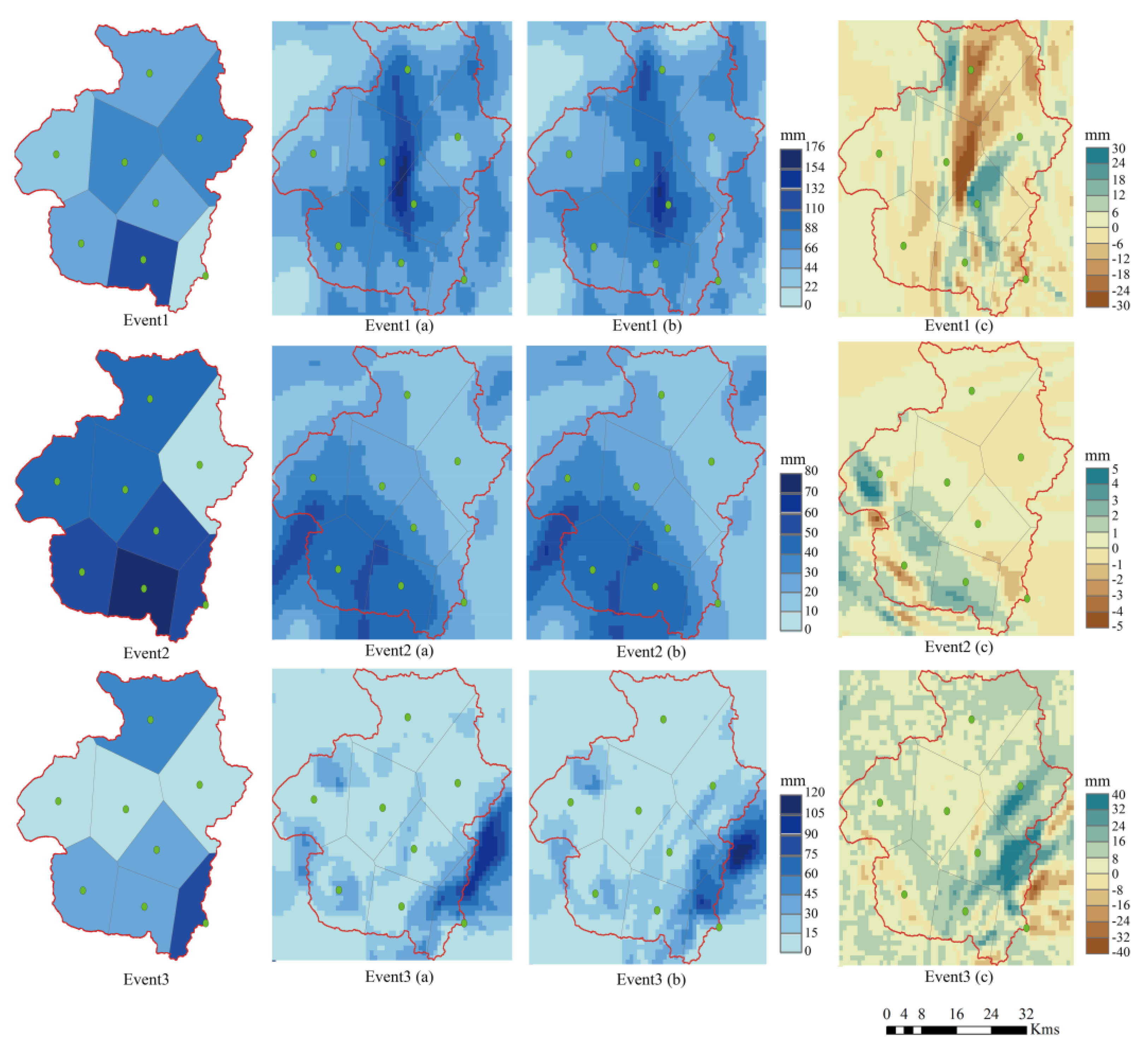
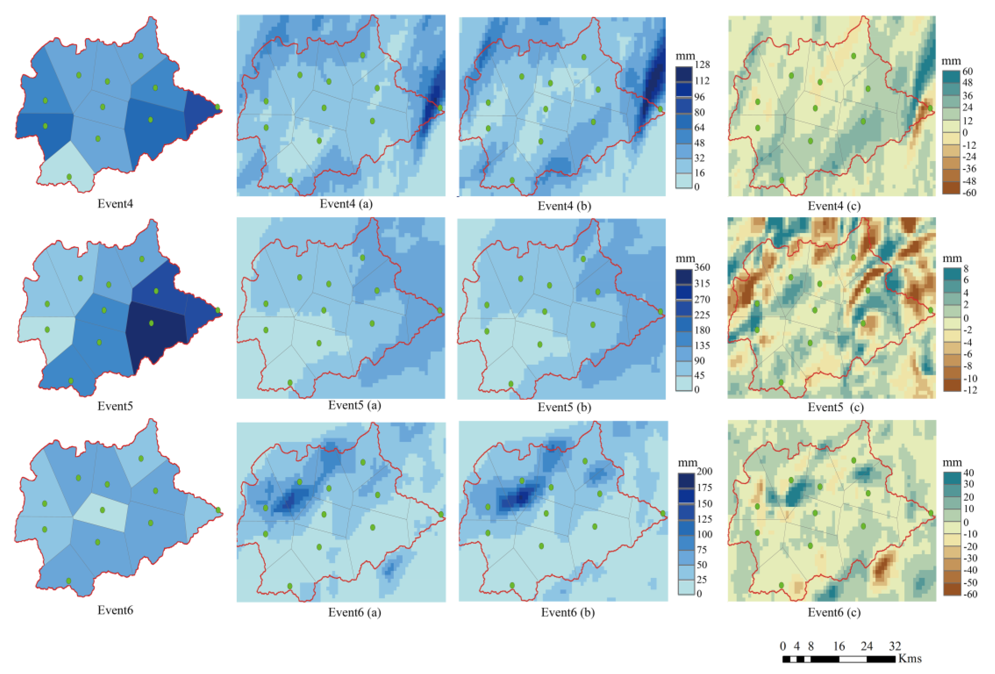
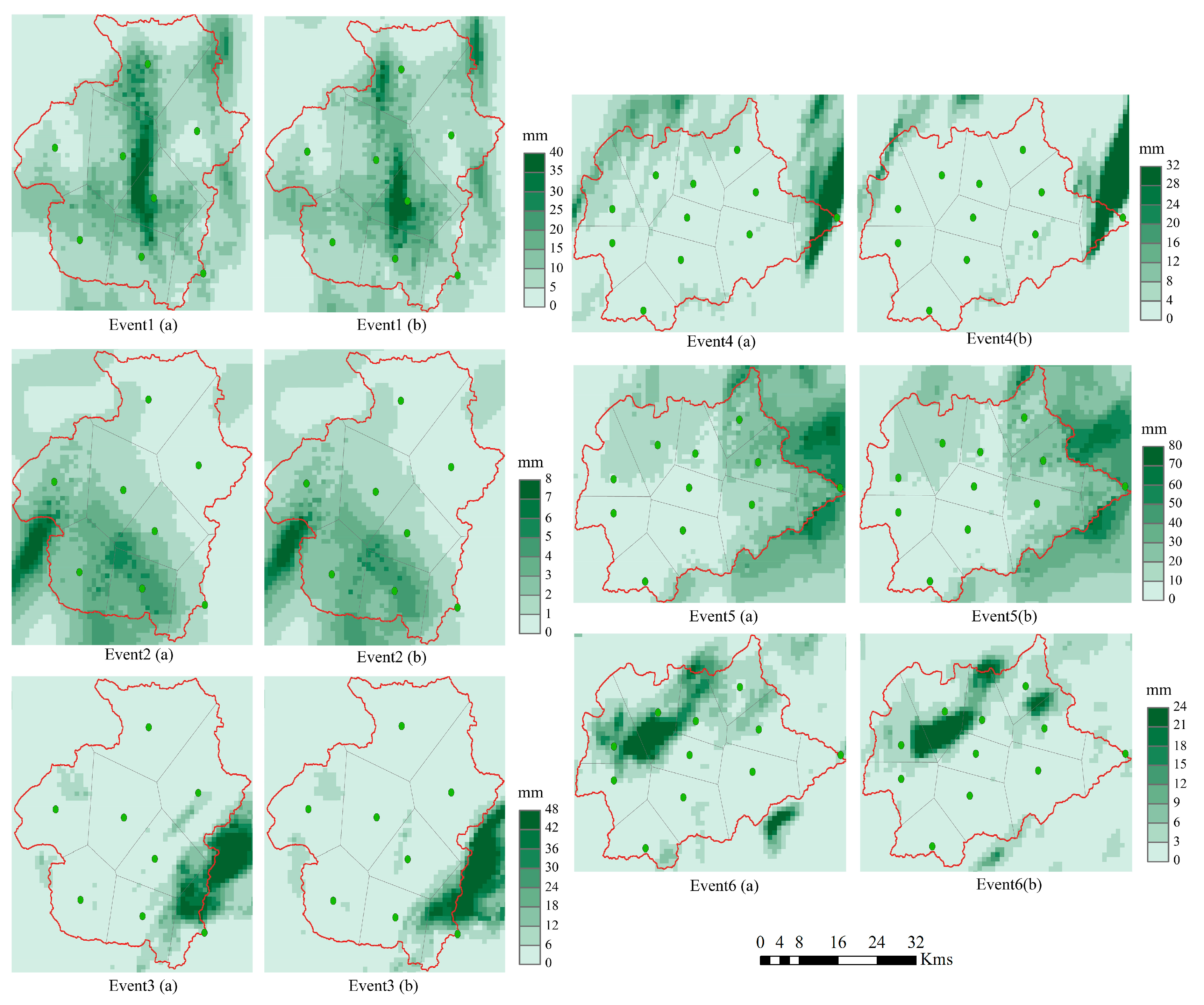
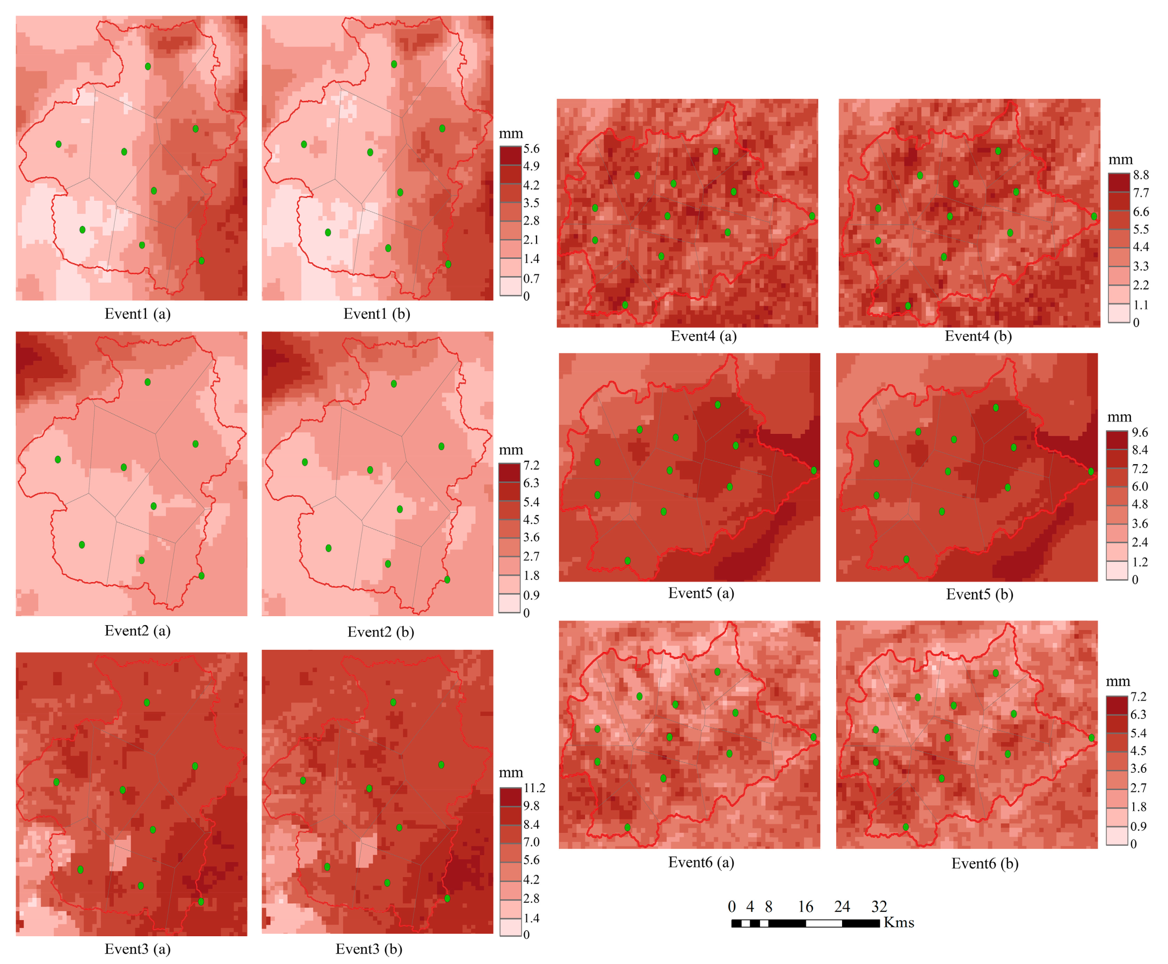
3.1.4. Spatial Variation of the Cumulative Rainfall

Figure 7 and Figure 8 illustrate the spatial variation of the 24 h cumulative rainfall in the Fuping and Zijingguan catchments. From left to right are the observed spatial patterns of the cumulative rainfall from the rain gauges, the simulated rainfall distribution of WRF-only and the fully coupled WRF/WRF-Hydro, and the spatial variations of the cumulative rainfall simulated by the two modes (i.e., the fully coupled WRF/WRF-Hydro minus WRF-only). Among all the subfigures (c), the spatial variations of Event 3, Event 4, and Event 6 were relatively more significant than the other events.
In particular, the coupled system simulations showed greater variations than WRF-only, which can be seen in the spatial variations in the subfigures (c) of Event 3, Event 4 and Event 6 (Type 3) and the fully coupled WRF/WRF-Hydro model improved WRF-only at the critical storm center due to its spatial redistribution of the rainfall. Spatially, the fully coupled WRF/WRF-Hydro and WRF-only showed essentially the same patterns for the cumulative rainfall distributions for both Type 1 and Type 2 events, and the simulations for the two events were better fitted with rain gauge observations than those of the Type 3 events. The storm centers of Event 1 and Event 2 were captured relatively well by the fully coupled WRF/WRF-Hydro as well as WRF-only. However, for Type 3 storm events, when matched with the observations, some parts of the catchments with high rainfall accumulations were missed by the fully coupled WRF/WRF-Hydro and WRF-only.
In comparison with WRF-only, Event 4 in the fully coupled WRF/WRF-Hydro was apart, with variations ranging from −60 mm to 60 mm as shown in Figure 8c, which raised the overall rainfall in the eastern and southern parts of Fuping and decreased the overall rainfall elsewhere. As a heavy convective historical storm, the rainfall intensity of Event 5 increased sharply in a very short period of time, with the maximum gauge cumulative values reaching up to 355 mm. The fully coupled WRF/WRF-Hydro underestimated this storm, and the WRF-only performed even worse, indicating a failure to capture these kinds of storm events in the Zijingguan catchment. The WRF-only had likewise the worst performance in reproducing the spatial rainfall distribution of Event 6, the storm center of which was dislocated. In stark contrast, the coupled system raised the rainfall in the north more than WRF-only for Event 6, with differences ranging from −60 mm to 40 mm, which showed a wider range than the differences of all other events, except those of Event 4. Event 4 and Event 6 occurred in relatively dry soil conditions in the previous period and there was no obvious rainfall in the catchment for nearly 15 days before the occurrence of the two storm events.

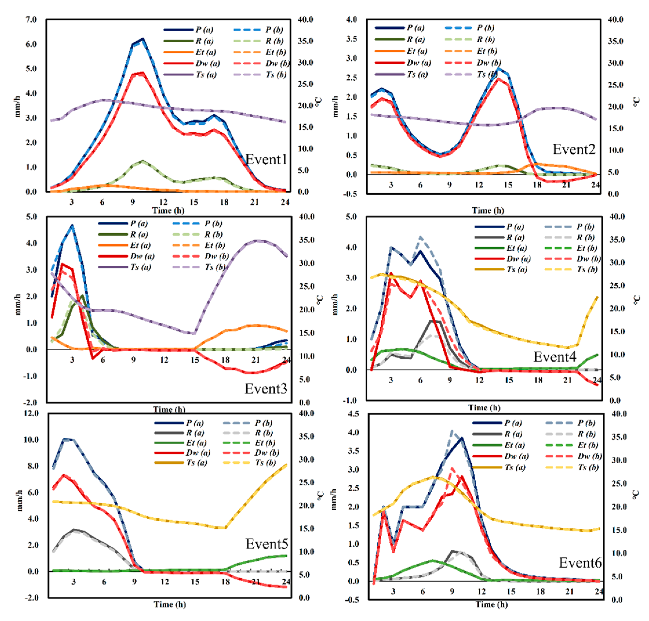
3.2. Simulations of Other Crucial Elements in the Water Cycle

3.2.1. Temporal Variation of the Water Cycle Elements

In addition to evaluating the spatiotemporal patterns of the rainfall, the spatiotemporal distribution variables of the other elements in water cycle were analyzed to understand the fully coupled system. These variables included evapotranspiration, runoff (the sum values of infiltration excess and saturated groundwater), water storage, and surface temperature. The basin water balance theory [22,51] was used in the calculation of the water storage change. This calculation can be expressed as follows:
Dw = PREt,
where Dw is the water storage change within 24 h for each flood event in the two catchments, and P, R, and Et are the rainfall, the generated runoff, and the evapotranspiration within the same time period, respectively.
For the analysis of the variables in the grid area, the 24 h changes can be seen in Figure 9. There were small amounts differed of the elements between WRF-only and the fully coupled WRF/WRF-Hydro as a short duration of 24 h. The R values of the fully coupled WRF/WRF-Hydro for the six events were less than that in WRF-only. In general, the fully coupled system increased the soil moisture and decreased the R. Note that the largest difference in R is Event 4 among all rainstorms, where the fully coupled WRF/WRF-Hydro was only 1.1 mm less than that of WRF-only. Compared to WRF-only, the coupled system Et values exhibited a decreasing trend, except for Event 2, which rose by only 0.001 mm. The amount of water storage slightly decreased in Type 1 and Type 2, while the water storage in the Type 3 events increased. At the same time, the change of the surface temperature within 24 h was not obvious, and the fluctuation range was quite narrow.
Figure 10 shows the graphs for the temporal variations of the grid average values of the crucial water cycle elements within 24 h. The Et trend was nearly the same as that of the Ts. During the period with high rainfall intensity, the Dw in the two catchments rose and Et increased until a stabilization in the later period. When the rainfall had gradually stopped, the Et increased with rising Ts (excepted for Event 1 and Event 6 with decreasing Ts), triggering the Dw decreasing to negative. For Event 4, and Event 6, the P and the Dw values generated by the fully coupled WRF/WRF-Hydro were slightly higher than those from WRF-only before and after the peak period.
A number of studies (e.g., Findell and Eltahir [52], and Koster et al. [53]) have argued that local soil moisture changes significantly in arid and semiarid regions dominated by convective rainfall, and such changes can affect the accuracy of a model simulation and reflect the Dw change to a certain extent. Figure 11 displays the hourly grid averaged soil moisture of the four soil layers (S1 to S4 with soil thickness ranges: 0–10 cm, 10–40 cm, 40–100 cm, 100–200 cm, respectively) simulated by the fully coupled WRF/WRF-Hydro and WRF-only, which are expressed in terms of the volumetric water content. That is, the values showed the average of the soil moisture in three dimensions including the grid, time, and layer number. For the soil layers in semi-humid watershed, due to the low soil moisture in the early stage and the short duration of the rainfall and infiltration processes, thinner S1 and S2 had a rapid soil moisture decrease due to high surface temperature and surface evaporation. Among 4 soil layers, soil moisture follows the rule that the attenuation gradually decreases with increasing layers. For S3 and S4, they have larger thickness and slower response. This could be reflected in Event 1, Event 3, and Event 5. Taking Event 5 as an example, the S1 in the first five hours of the storm reached nearly 0.4 from around 0.3, and it was then maintained at a high level for the next five hours. The same thing happened for the other three events, and only S1 and S2 changed.
The fully coupled WRF/WRF-Hydro soil moisture values all exceeded WRF-only values. For S1 and S2 in Event 4 and Event 6, there was higher S1 and S2 before and after the peak period, which might be used as an explanation for the sudden increase of P and Dw in Figure 10. In the coupling WRF-Hydro system, soil moisture, as a key feedback variable, could affect the spatial fluctuation range of precipitation. Compared with the accumulative difference of rainfall, we found that a larger fluctuation corresponded to initial drier soil conditions (Figure 7c, Figure 8 c, Figure 11). The more soil moisture the columnar soil layer lacks, the more the hydrological module could feedback to the land surface system and WRF to affect the elements spatiotemporal distribution in the fully coupled system.

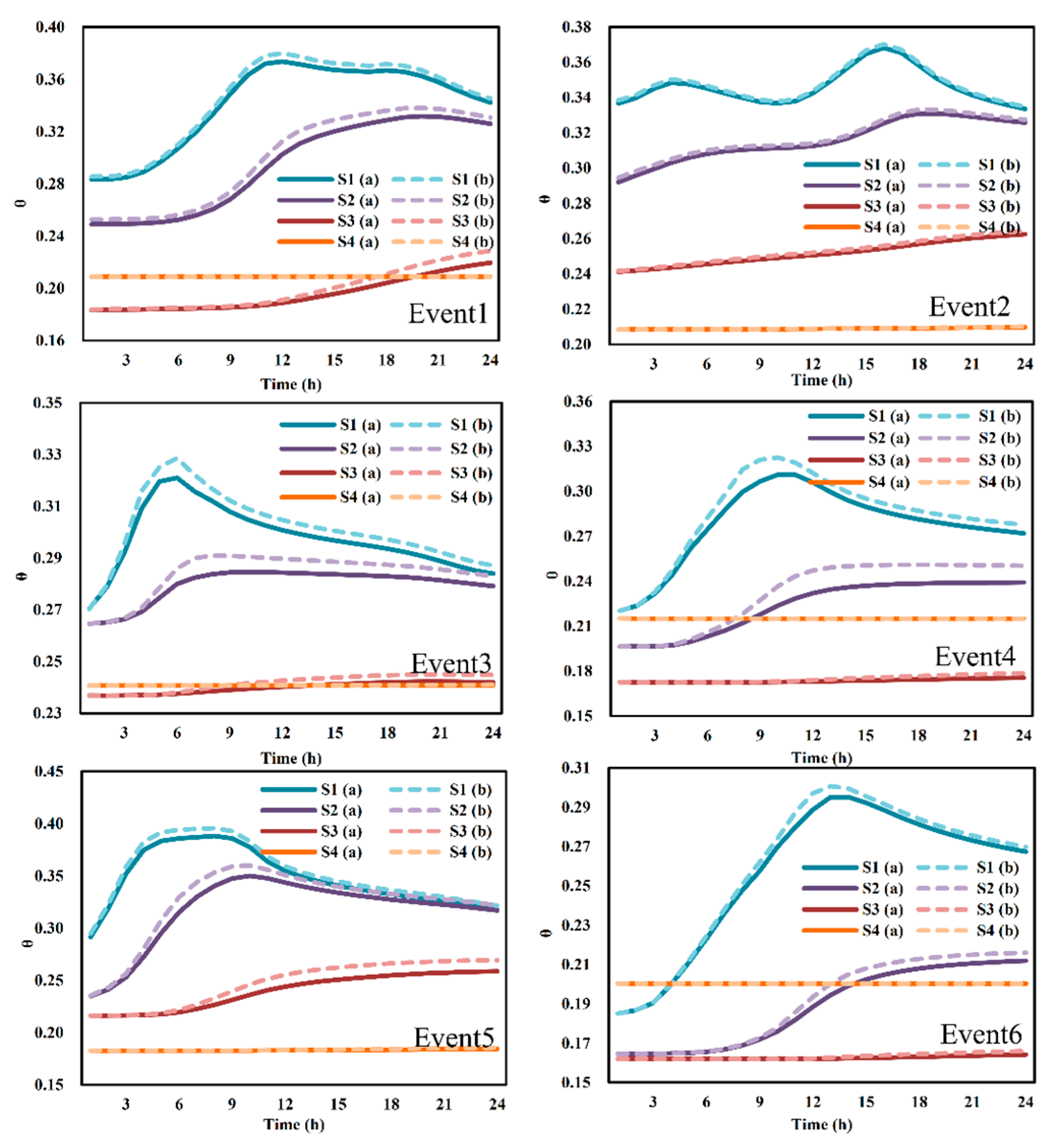
3.2.2. Spatial Variation of the Soil Moisture

Figure 12 shows the hourly averaged soil moisture of the four soil layers. It can be seen that the values of Event 4 and Event 6 were much less than the values of the other events in the whole rainfall period. The spatial distributions of the soil moisture were the same as the cumulative rainfall for both WRF-only and the fully coupled WRF/WRF-Hydro, as the soil based on the higher accumulated rainfall was more humid. However, in comparison with WRF-only, the fully coupled system generally produced higher soil moisture content. The soil moisture of the storm center simulated by the fully coupled WRF/WRF-Hydro increased more than that of WRF-only, especially for Event 1, Event 3, and Event 5. This may also be the reason for the lower R values of the fully coupled WRF/WRF-Hydro.

3.2.3. Spatial Variation of the Cumulative Runoff

The runoff of the fully coupled system is determined by both precipitation and soil moisture, as the variables transferred back to Noah by the hydrological module of the fully coupled system include the water accumulation depth and soil moisture content of each soil layer. The spatial distributions of the 24 h cumulative runoff are shown in Figure 13, for which both WRF-only and the coupled WRF/WRF-Hydro were generally consistent with the rainfall, and high runoff values in places with high rainfall as well. The generated runoff of the storm center simulated by the two systems was higher than the other regions of the study catchments. Event 5 had the greatest rainfall accumulation, and the local maximum runoff was almost 80 mm, while Event 2 had the least cumulative rainfall, and the local runoff was just 8 mm. At the same time, the volume of the generated runoff was also subject to the change in the local soil moisture. With relatively dry soil conditions such as Event 4 and Event 6, it can be seen from Figure 12 that when the soil moisture was less than 0.26, the generated runoff was also relatively low. Besides this, the runoff changed from the WRF-only to the coupled WRF/WRF-Hydro, and Event 3, Event 4, and Event 6 in particular could reflect subtle differences similar to the rainfall.

3.2.4. Spatial Variation of the Cumulative Evapotranspiration

The spatial variation of the Et between WRF-only and the fully coupled WRF/WRF-Hydro was far from consisting of the rainfall spatial distribution. Figure 14 shows the 24 h average spatial distribution of Et. The Et range of Event 1 was the narrowest, from 0–5.6 mm, while the range of Event 3 was the broadest, from 0–11.2 mm. For Event 3 and Event 5, which reached their peaks (Figure 10) in the first few hours, the spatial distribution of Et was consistent with the rainfall. For the rest of the events, the spatial distribution of the Et was different from the rainfall distribution. Especially for Event 4 and Event 6 with relatively dry soil conditions, the cases were more complicated. In fact, ET was affected not only by the rainfall and the soil moisture, but also by many other factors, e.g., the soil temperature, the latent heat fluxes, the air pressure and the wind speed, etc. In the early stage of the storm, the soil moisture was spatially inhomogeneous, and with the growth of the soil moisture, the evapotranspiration rapidly increased. When the rainfall gradually stopped, the soil moisture decreased and became spatially stable, and the evapotranspiration continued across the catchment. If there were no particularly strong interference factors in the subsequent time period, the evapotranspiration of each grid cell would gradually tend toward a stable value.

4. Discussion

Enhanced hydrological representations on short-term meteorological forecasts are more uncertain, and as yet under investigation and understanding its impact [25]. The concept of coupling the hydrological model (WRF-Hydro) with atmospheric model (WRF) was expected to reduce uncertainties associated with the spatial and temporal distribution of storm events, especially for complex terrain. In this study, six storm events were screened with different spatiotemporal characteristics during a 24-hour window. The focus is to explore the short-term temporal and spatial water exchanges of elements in the water cycle, especially different spatiotemporal types rainfall between WRF-only and the coupled WRF/WRF-hydro in the semi-humid areas of northern China, where the short real rainfall duration is regarded as a great challenge to the coupled system. Through categorical and continuous indices, we proved a potential for the fully coupled system to reduce spatial mean square error and could be confirmed from the enhancement spatial distribution of precipitation in the fully coupled WRF-Hydro, especially for the simulation of rainstorm centers. However, when the fully coupled WRF/WRF-Hydro is used, attention should be paid to the false alarm risk of rainfall occurrences and period rainfall values in time inhomogeneous storms which have large rainfall intensity.
The distribution of precipitation among land water cycle elements is a complex process, and more details are not yet fully explored [54]. In our study, the redistributions fluctuation of spatial precipitation in the fully coupled system was highly correlated with soil moisture, and a low initial soil moisture corresponded to a large spatial fluctuated range. The feedback process of the increased soil moisture after the spatial redistribution led to the increase in precipitation in the corresponding position, indicating that there may be a positive feedback relationship between local soil moisture and precipitation. The spatial redistribution of soil moisture will change the surface flux, which may affect boundary layer dynamics, the initiation of moist convection and precipitation [55,56]. In this study, the fully coupled system generally produced higher soil moisture content than WRF-only. This was consistent with the previous study by Senatore et al. [25], which claimed before that the reason was related to the combined effects of lateral terrestrial water flow redistribution in the fully coupled system by allowing more water to circulate in the regional water cycle.
The fully coupled system is unstable and far from maturity [57]. After a disaggregation of the land surface module, the coupled WRF-Hydro carries out the overland and undersurface routing on a finer grid, and then, through average of the subgrid, aggregates and feeds back to the LSM to realize the horizontal interaction between the hydrological module and LSM. It solves the spatial variability structure of soil moisture resolution from one to the next time step. One of the model structure restraints is that even if there are adjustable thicknesses of four soil layers in WRF-Hydro, they are constant throughout the entire model domain. This does not bring much trouble to this study due to the relatively single local soil type (cinnamon soil), but for the areas with strong soil heterogeneity, it is still a problem to be solved because the main runoff generation processes are carried out in the ‘fixed column’.
Since the primary objective of the study is to show the effects of different spatiotemporal types rainfall between WRF-only and the fully coupled WRF/WRF-Hydro in the semi-humid areas of northern China, rather than extensively assessing the performance of the hydrological module, the streamflow is limited to only a simple foregoing calibration of four sensitivity parameters in the stand-alone WRF-Hydro. The lateral redistribution process includes the overland routing and subsurface routing, which means the runoff process will not be regulated by the feedback of the channel routing. On the contrary, the streamflow is affected by the runoff. The comparison of runoff processes could reflect the difference between the fully coupled WRF/WRF-Hydro and WRF-only. In fact, except for Event 1, there was general underestimated streamflow in the standalone WRF-Hydro calibration compared to the observations, which might be because of the underestimated accumulative rainfall of forcing data from WRF and insufficient response to the channel characteristics parameters. It should be mentioned that the simulations of WRF-only and the fully coupled system were all based on one set of physical parameterizations which was found to be adaptive to most of the storm events in the study area [29]. One can notice that for some events, the simulated rainfall and other variables by the WRF model had some considerable errors, which were inevitably caused by the forcing data or the parameterization schemes. The accuracy of the forcing data could be a significant factor restricting the performance of the atmospheric-hydrologic coupling system. Precise spatiotemporal information about the storm center and the soil moisture (e.g., radar-rain gauge merging methods, soil moisture data assimilation) may help provide improved simulations of the terrestrial atmospheric and hydrological processes.
The topographic and climatic characteristics of study area make it strenuous to screen enough homogeneous events, and increase the uncertainty of the simulations. When applying the fully coupled WRF/WRF-Hydro modeling system, the determination of model parameter, the spatial static data, the integration time step, and the downscaling resolution may all have some impact on the final results. The generalization of the conclusions in this study may also be restricted to some extent by the above issues as same as indicate some prospects for future studies.

5. Conclusions

To enhance the understanding of the hydrometeorological conditions in semi-humid area of northern China, six rainfall events that occurred in two medium-scale catchments were sorted with different homogeneousness in space and time. The spatiotemporal characteristics of rainfall and several key water cycle elements (e.g., soil moisture, evapotranspiration and generated surface runoff) were investigated by the stand-alone WRF model and the fully coupled WRF/WRF-Hydro modeling system. We proved that the precipitation events in the fully coupled system were slightly improved than those in WRF-only, and the simulation performances were related with the temporal and spatial homogeneousness of storm events. For both WRF-only and the fully coupled WRF/WRF-Hydro, the events with inhomogeneous spatiotemporal distributions of rainfall could lead to somewhat worse simulations than those with homogeneous rainfall distributions in space or time and both the two modeling simulations showed to be more realistic in space than in time. The fully coupled system could improve the spatial distribution, especially the advantage of a lower mean bias error and the enhanced prediction of rainstorm center than WRF-only. In the fully coupled system, the fluctuation of precipitation was corresponded to the initial soil moisture, and for the temporal inhomogeneous precipitation, the system might produce a large false alarm than WRF-only. Compared with WRF-only, the simulations of the crucial water cycle elements by the fully coupled system differed with relatively small amounts in the average of two catchments and generally increased soil moisture and decreased surface runoff. The spatial distributions in the fully coupled system were redistributed and the generated runoff and the soil moisture was generally consistent with that of the cumulative rainfall, while the evapotranspiration did not always show the same trend due to more complicated influencing mechanisms.
For semi-humid areas, how to exactly capture the rainfall process with inhomogeneous distributions in space and time or with precedent dry soil conditions is the key point to be solved in the following study.

Author Contributions

Conceptualization, W.W. and J.L.; methodology, W.W. and F.Y.; software, W.W. and Y.L.; validation, W.W. and Y.L.; formal analysis, W.W. and J.L.; investigation, W.W. and F.Y.; writing—original draft preparation, W.W. and J.L.; writing—review and editing, W.W., J.L. and C.L.; visualization, W.W. and E.Y.; funding acquisition, J.L. and C.L. All authors have read and agreed to the published version of the manuscript.

Funding

This research was funded by the Major Science and Technology Program for Water Pollution Control and Treatment (2018ZX07110001), the National Natural Science Foundation of China (51822906), the National Key Research and Development Project (2017YFC1502405), and the IWHR Research & Development Support Program (WR0145B732017).

Conflicts of Interest

The authors declare no conflict of interest.

References

  1. Nasri, S.; Cudennec, C.; Albergel, J.; Berndtsson, R. Use of a geomorphological transfer function to model design floods in small hillside catchments in semiarid Tunisia. J. Hydrol. 2004, 287, 197–213. [Google Scholar] [CrossRef]
  2. Nikolopoulos, E.I.; Anagnostou, E.N.; Hossain, F.; Gebremichael, M.; Borga, M. Understanding the Scale Relationships of Uncertainty Propagation of Satellite Rainfall through a Distributed Hydrologic Model. J. Hydrometeorol. 2010, 11, 520–532. [Google Scholar] [CrossRef]
  3. Srivastava, P.K.; Han, D.; Rico-Ramirez, M.A.; Islam, T. Sensitivity and uncertainty analysis of mesoscale model downscaled hydro-meteorological variables for discharge prediction. Hydrol. Process. 2014, 28, 4419–4432. [Google Scholar] [CrossRef]
  4. Hanel, M.; Buishand, T.A. On the value of hourly precipitation extremes in regional climate model simulations. J. Hydrol. 2010, 393, 265–273. [Google Scholar] [CrossRef]
  5. Jiao, Y.; Lei, H.; Yang, D.; Huang, M.; Liu, D.; Yuan, X. Impact of vegetation dynamics on hydrological processes in a semi-arid basin by using a land surface-hydrology coupled model. J. Hydrol. 2017, 551, 116–131. [Google Scholar] [CrossRef]
  6. Kerandi, N.; Arnault, J.; Laux, P.; Wagner, S.; Kitheka, J.; Kunstmann, H. Joint atmospheric-terrestrial water balances for East Africa: A WRF-Hydro case study for the upper Tana River basin. Theor. Appl. Climatol. 2018, 131, 1337–1355. [Google Scholar] [CrossRef] [Green Version]
  7. Kurtzman, D.; Navon, S.; Morin, E. Improving interpolation of daily precipitation for hydrologic modelling: Spatial patterns of preferred interpolators. Hydrol. Process. 2010, 23, 3281–3291. [Google Scholar] [CrossRef]
  8. Shrestha, K.Y.; Webster, P.J.; Toma, V.E. An Atmospheric-Hydrologic Forecasting Scheme for the Indus River Basin. J. Hydrometeorol. 2014, 15, 861–890. [Google Scholar] [CrossRef]
  9. Wen, X.; Lu, S.; Jin, J. Integrating Remote Sensing Data with WRF for Improved Simulations of Oasis Effects on Local Weather Processes over an Arid Region in Northwestern China. J. Hydrometeorol. 2012, 13, 573–587. [Google Scholar] [CrossRef]
  10. Sato, T.; Kimura, F.; Kitoh, A. Projection of global warming onto regional precipitation over Mongolia using a regional climate model. J. Hydrol. 2007, 333, 144–154. [Google Scholar] [CrossRef]
  11. Welch, R.M.; Kuo, K.S.; Sengupta, S.K.; Wielicki, B.A.; Parker, L. Marine stratocumulus cloud fields off the coast of southern California observed using Landsat imagery. I: Structural characteristics. J. Appl. Meteorol. 1988, 27, 341–362. [Google Scholar] [CrossRef] [Green Version]
  12. Niu, G.Y.; Yang, Z.L.; Mitchell, K.E.; Chen, F.; Ek, M.B.; Barlage, M.; Kumar, A.; Manning, K.; Niyogi, D.; Rosero, E. The community Noah land surface model with multiparameterization options (Noah-MP): 1. Model description and evaluation with local-scale measurements. J. Geophys. Res. Atmos. 2011, 116, 1248–1256. [Google Scholar] [CrossRef] [Green Version]
  13. Van Den Broeke, M.S.; Kalin, A.; Alavez, J.A.T.; Oglesby, R.; Hu, Q. A warm-season comparison of WRF coupled to the CLM4.0, Noah-MP, and Bucket hydrology land surface schemes over the central USA. Theor. Appl. Climatol. 2018, 134, 801–816. [Google Scholar] [CrossRef] [Green Version]
  14. Yu, Z.; Lakhtakia, M.N.; Yarnal, B.; White, R.A.; Miller, D.A.; Frakes, B.; Barron, E.J.; Duffy, C.; Schwartz, F.W. Simulating the river-basin response to atmospheric forcing by linking a mesoscale meteorological model and hydrologic model system. J. Hydrol. 1999, 218, 72–91. [Google Scholar] [CrossRef]
  15. Zabel, F.; Mauser, W. 2-way coupling the hydrological land surface model PROMET with the regional climate model MM5. Hydrol. Earth Syst. Sci. 2013, 17, 1705–1714. [Google Scholar] [CrossRef] [Green Version]
  16. Zhongbo, Y.U.; Pollard, D.; Cheng, L.I. On continental-scale hydrologic simulations with a coupled hydrologic model. J. Hydrol. 2006, 331, 110–124. [Google Scholar] [CrossRef]
  17. Maxwell, R.M.; Chow, F.K.; Kollet, S.J. The groundwater–land-surface–atmosphere connection: Soil moisture effects on the atmospheric boundary layer in fully-coupled simulations. Adv. Water Res. 2007, 30, 2447–2466. [Google Scholar] [CrossRef] [Green Version]
  18. Kollet, S.J.; Maxwell, R.M. Integrated surface–groundwater flow modeling: A free-surface overland flow boundary condition in a parallel groundwater flow model. Adv. Water Res. 2006, 29, 945–958. [Google Scholar] [CrossRef] [Green Version]
  19. Xue, M.; Droegemeier, K.K.; Wong, V. The Advanced Regional Prediction System (ARPS)–A multi-scale nonhydrostatic atmospheric simulation and prediction model. Part I: Model dynamics and verification. Meteorol. Atmos. Phys. 2000, 75, 161–193. [Google Scholar] [CrossRef]
  20. Maxwell, R.M.; Lundquist, J.K.; Mirocha, J.D.; Smith, S.G.; Tompson, A.F.B. Development of a Coupled Groundwater-Atmosphere Model. Mon. Weather Rev. 2011, 139, 96–116. [Google Scholar] [CrossRef]
  21. Gochis, D.J.; Yu, W.; Yates, D.N. The WRF-Hydro Model Technical Description and User’s Guide, Version 3.0. NCAR Technical Document. 120 pages. Available online: https://ral.ucar.edu/projects/wrf_hydro/technical-description-user-guide (accessed on 24 April 2020).
  22. Lu, L.; Gochis, D.J.; Sobolowksi, S.; Mesquita, M.D.S. Evaluating the present annual water budget of a Himalayan headwater river basin using a high-resolution atmosphere-hydrology model. J. Geophys. Res. Atmos. 2017, 122, 4786–4807. [Google Scholar] [CrossRef]
  23. Lin, P.R.; Rajib, M.A.; Yang, Z.L.; Somos-Valenzuela, M.; Merwade, V.; Maidment, D.R.; Wang, Y.; Chen, L. Spatiotemporal Evaluation of Simulated Evapotranspiration and Streamflow over Texas Using the WRF-Hydro-RAPID Modeling Framework. J. Am. Water Resour. As. 2018, 54, 40–54. [Google Scholar] [CrossRef]
  24. Xiang, T.T.; Vivoni, E.R.; Gochis, D.J.; Mascaro, G. On the diurnal cycle of surface energy fluxes in the North American monsoon region using the WRF-Hydro modeling system. J. Geophys. Res. Atmos. 2017, 122, 9024–9049. [Google Scholar] [CrossRef]
  25. Senatore, A.; Mendicino, G.; Gochis, D.J.; Yu, W.; Yates, D.N.; Kunstmann, H. Fully coupled atmosphere-hydrology simulations for the central Mediterranean: Impact of enhanced hydrological parameterization for short and long time scales. J. Adv. Model. Earth Syst. 2015, 7, 1693–1715. [Google Scholar] [CrossRef]
  26. Xiang, T.; Vivoni, E.; Gochis, D. Influence of Initial Soil Moisture and Vegetation Conditions on Monsoon Precipitation Events in Northwest Mexico. Atmosfera 2017, 31. [Google Scholar] [CrossRef] [Green Version]
  27. Wehbe, Y.; Temimi, M.; Weston, M.; Chaouch, N.; Branch, O.; Schwitalla, T.; Wulfmeyer, V.; Zhan, X.; Liu, J.; Al Mandous, A. Analysis of an extreme weather event in a hyper-arid region using WRF-Hydro coupling, station, and satellite data. Nat. Hazards Earth Syst. Sci. 2019, 19, 1129–1149. [Google Scholar] [CrossRef] [Green Version]
  28. Liu, J.; Bray, M.; Han, D. Sensitivity of the Weather Research and Forecasting (WRF) model to downscaling ratios and storm types in rainfall simulation. Hydrol. Process. 2012, 26, 3012–3031. [Google Scholar] [CrossRef]
  29. Tian, J.; Liu, J.; Wang, J.; Li, C.; Yu, F.; Chu, Z. A spatio-temporal evaluation of the WRF physical parameterisations for numerical rainfall simulation in semi-humid and semi-arid catchments of Northern China. Atmos. Res. 2017, 191, 141–155. [Google Scholar] [CrossRef]
  30. Cardoso, R.M.; Soares, P.M.M.; Miranda, P.M.A.; Belo-Pereira, M. WRF high resolution simulation of Iberian mean and extreme precipitation climate. Int. J. Climatol. 2013, 33, 2591–2608. [Google Scholar] [CrossRef]
  31. Qian, Y.; Ghan, S.J.; Leung, L.R. Downscaling hydroclimatic changes over the Western US based on CAM subgrid scheme and WRF regional climate simulations. Int. J. Climatol. 2009, 30. [Google Scholar] [CrossRef]
  32. Toride, K.; Iseri, Y.; Duren, A.M.; England, J.F.; Kavvas, M.L. Evaluation of physical parameterizations for atmospheric river induced precipitation and application to long-term reconstruction based on three reanalysis datasets in Western Oregon. Sci. Total Environ. 2018, 658, 570–581. [Google Scholar] [CrossRef]
  33. Wang, X.; Barker, D.M.; Snyder, C.; Hamill, T.M. A Hybrid ETKF–3DVAR data assimilation scheme for the WRF model. Part I: Observing system simulation experiment. Mon. Weather Rev. 2007, 136, 5116–5131. [Google Scholar] [CrossRef] [Green Version]
  34. Hong, S.; Noh, Y.; Dudhia, J. A New Vertical Diffusion Package with an Explicit Treatment of Entrainment Processes. Mon. Weather Rev. 2006, 134, 2318–2341. [Google Scholar] [CrossRef] [Green Version]
  35. Kain, J.S. The Kain-Fritsch Convective Parameterization: An Update. J. Appl. Meteorol. 2004, 43, 170–181. [Google Scholar] [CrossRef] [Green Version]
  36. Lin, Y.; Farley, R.D.; Orville, H.D. Bulk Parameterization of the Snow Field in a Cloud Model. J. Appl. Meteorol. 1983, 22, 1065–1092. [Google Scholar] [CrossRef] [Green Version]
  37. Skamarock, W. A Description of the Advanced Research WRF Version 3. NCAR Tech. Note; NCAR/TN-475+ STR; University Corporation for Atmospheric Research: Boulder, CO, USA, 2008. [Google Scholar] [CrossRef] [Green Version]
  38. Ek, M.B.; Mitchell, K.E.; Lin, Y.Y.; Rogers, E.; Grunmann, P.; Koren, V.; Gayno, G.; Tarpley, J.D. Implementation of Noah land surface model advances in the National Centres for Environmental Prediction operational mesoscale Eta model. J. Geophys. Res. 2003, 108, 8851. [Google Scholar] [CrossRef]
  39. Warrach-Sagi, K.; Schwitalla, T.; Wulfmeyer, V.; Bauer, H.-S. Evaluation of a climate simulation in Europe based on the WRF–NOAH model system: Precipitation in Germany. Clim. Dyn. 2013, 41, 755–774. [Google Scholar] [CrossRef] [Green Version]
  40. Research Applications Laboratory of National Center for Atmospheric Research. Available online: https://ral.ucar.edu/projects/wrf_hydro/overview (accessed on 22 April 2020).
  41. Schaake, J.C.; Koren, V.I.; Duan, Q.-Y.; Mitchell, K.; Chen, F. Simple water balance model for estimating runoff at different spatial and temporal scales. J. Geophys. Res. Atmos. 1996, 101, 7461–7475. [Google Scholar] [CrossRef]
  42. Downer, C.W.; Ogden, F.L.; Martin, W.D.; Harmon, R.S. Theory, development, and applicability of the surface water hydrologic model CASC2D. Hydrol. Process. 2002, 16, 255–275. [Google Scholar] [CrossRef]
  43. Wigmosta, M.S.; Lettenmaier, D.P. A comparison of simplified methods for routing topographically driven subsurface flow. Water Resour. Res. 1999, 35, 255–264. [Google Scholar] [CrossRef]
  44. Gochis, D.J.; Chen, F. Hydrological Enhancements to the Community Noah Land Surface Model; University Corporation for Atmospheric Research: Boulder, CO, USA, 2002. [Google Scholar] [CrossRef]
  45. Naabil, E.; Lamptey, B.L.; Arnault, J.; Olufayo, A.; Kunstmann, H. Water resources management using the WRF-Hydro modelling system: Case-study of the Tono dam in West Africa. J. Hydrol. 2017, 12, 196–209. [Google Scholar] [CrossRef]
  46. Ryu, Y.; Lim, Y.J.; Ji, H.S.; Park, H.H.; Chang, E.C.; Kim, B.J. Applying a coupled hydrometeorological simulation system to flash flood forecasting over the Korean Peninsula. Asia Pac. J. Atmos. Sci. 2017, 53, 421–430. [Google Scholar] [CrossRef]
  47. Yucel, I.; Onen, A.; Yilmaz, K.K.; Gochis, D.J. Calibration and evaluation of a flood forecasting system: Utility of numerical weather prediction model, data assimilation and satellite-based rainfall. J. Hydrol. 2015, 523, 49–66. [Google Scholar] [CrossRef] [Green Version]
  48. Sivapalan, M.; Bloschl, G. Transformation of point rainfall to areal rainfall: Intensity-duration- frequency curves. J. Hydrol. 1998, 204, 150–167. [Google Scholar] [CrossRef]
  49. Jolliffe, I.T.; Stephenson, D.B. Forecast Verification: A Practitioner’s Guide in Atmospheric Science, 2nd ed.; Academic Press: Burlington, MA, USA, 2003. [Google Scholar] [CrossRef]
  50. Wilks, D.S. Statistical Methods in Atmospheric Science, 2nd ed.; Academic Press: Burlington, MA, USA, 2006. [Google Scholar] [CrossRef]
  51. Oki, T.; Musiake, K.; Matsuyama, H.; Masuda, K. Global atmospheric water balance and runoff from large river basins. Hydrol. Process. 1995, 9, 655–678. [Google Scholar] [CrossRef]
  52. Findell, K.L.; Eltahir, E.A.B. Atmospheric Controls on Soil Moisture–Boundary Layer Interactions. Part I: Framework Development. J. Hydrometeorol. 2003, 4, 552–569. [Google Scholar] [CrossRef]
  53. Koster, R.D.; Dirmeyer, P.A.; Zhichang, G.; Gordon, B.; Edmond, C.; Peter, C.; Gordon, C.T.; Shinjiro, K.; Eva, K.; David, L. Regions of strong coupling between soil moisture and precipitation. Science 2004, 305, 1138–1140. [Google Scholar] [CrossRef] [Green Version]
  54. Brooks, P.D.; Chorover, J.; Fan, Y.; Godsey, S.E.; Maxwell, R.M.; McNamara, J.P.; Tague, C. Hydrological partitioning in the critical zone: Recent advances and opportunities for developing transferable understanding of water cycle dynamics. Water Resour. Res. 2015, 51, 6973–6987. [Google Scholar] [CrossRef] [Green Version]
  55. Pielke, R.A., Sr. Influence of the spatial distribution of vegetation and soils on the prediction of cumulus convective rainfall. Rev. Geophys. 2001, 39, 151–177. [Google Scholar] [CrossRef]
  56. Arnault, J.; Rummler, T.; Baur, F.; Lerch, S.; Wagner, S.; Fersch, B.; Zhang, Z.; Kerandi, N.; Keil, C.; Kunstmann, H. Precipitation sensitivity to the uncertainty of terrestrial water flow in WRF-Hydro: An ensemble analysis for Central Europe. J. Hydrometeorol. 2018, 19, 1007–1025. [Google Scholar] [CrossRef]
  57. Fersch, B.; Senatore, A.; Adler, B.; Arnault, J.; Mauder, M.; Schneider, K.; Völksch, I.; Kunstmann, H. High-resolution fully-coupled atmospheric–hydrological modeling: A cross-compartment regional water and energy cycle evaluation. Hydrol. Earth Syst. Sci. Discuss. 2019, 478, 1–37. [Google Scholar] [CrossRef] [Green Version]
Figure 1. Locations and digital elevation models (DEMs) of the two study catchments in northern China with the gauges and the settings of the Weather Research and Forecasting model (WRF) nested domains.
Water 12 01209 g001
Figure 2. The observed and simulated 24 h rainfall accumulations for the six storm events.
Water 12 01209 g002
Figure 3. Evaluation values of the indices for the temporal rainfall distribution of the six storm events: (a) WRF-only; (b) the fully coupled WRF/WRF-Hydro.
Water 12 01209 g003
Figure 4. Temporal heat map of the indices error: (a) WRF-only; (b) the fully coupled WRF/WRF-Hydro.
Water 12 01209 g004
Figure 5. Evaluation values of the indices for the spatial rainfall distribution of the six storm events: (a) WRF-only; (b) the fully coupled WRF/WRF-Hydro.
Water 12 01209 g005
Figure 6. Spatial heat map of the indices errors: (a) WRF-only; (b) the fully coupled WRF/WRF-Hydro.
Water 12 01209 g006
Figure 7. Spatial distributions of the 24 h accumulative rainfall for the three storm events in the Fuping catchment, from left to right: gauge observation; (a) WRF-only; (b) the fully coupled WRF/WRF-Hydro; (c) the fully coupled WRF/WRF-Hydro minus WRF-only.
Water 12 01209 g007
Figure 8. Spatial distributions of the 24 h accumulative rainfall for the three storm events in the Zijingguan catchment, from left to right: gauge observation; (a) WRF-only; (b) the fully coupled WRF/WRF-Hydro; (c) the fully coupled WRF/WRF-Hydro minus WRF-only.
Water 12 01209 g008
Figure 9. Heat map of grid average values of the crucial elements in the water cycle: (a) WRF-only; (b) the fully coupled WRF/WRF-Hydro; P, R, Et and Dw are the statistics for the 24 h cumulative values (mm), and Ts represents the hourly grid averaged values (°C).
Water 12 01209 g009
Figure 10. Temporal variations of the grid average values for the crucial elements in the water cycle: (a) WRF-only; (b) the fully coupled WRF/WRF-Hydro.
Water 12 01209 g010
Figure 11. Temporal variations of the grid average soil moisture in the four soil layers: (a) WRF-only; (b) the fully coupled WRF/WRF-Hydro.
Water 12 01209 g011
Figure 12. Spatial distributions of the hourly averaged soil moisture of the four soil layers: (a) WRF-only; (b) the fully coupled WRF/WRF-Hydro.
Water 12 01209 g012
Figure 13. Spatial distributions of the 24 h cumulative runoff of the four soil layers: (a) WRF-only; (b) the fully coupled WRF/WRF-Hydro.
Water 12 01209 g013
Figure 14. Spatial distributions of the 24 h cumulative evapotranspiration: (a) WRF-only; (b) the fully coupled WRF/WRF-Hydro.
Water 12 01209 g014
Table 1. Storm events selected from the two study catchments and their spatiotemporal rainfall evenness characterized by Cv.
Event IDCatchmentRainfall WindowAccumulated
24 h Rainfall (mm)
Spatial CvTemporal CvType Label
1Fuping07/29/2007 20:00 to 07/30/2007 20:0063.40.4000.6011
2Fuping07/30/2012 10:00 to 07/31/2012 10:0050.50.1931.0822
3Fuping08/11/2013 07:00 to 08/12/2013 07:0030.90.7402.3933
4Zijingguan08/10/2008 00:00 to 08/11/2008 00:0045.50.4591.378
5Zijingguan07/21/2012 04:00 to 07/22/2012 04:00172.20.6101.887
6Zijingguan06/06/2013 22:00 to 06/07/2013 22:0052.10.4261.887
Table 2. Configurations of the WRF model.
SubjectChosen OptionSubjectChosen Option
Driving data6 h FNLPressure50 hPa
Integration time-step6 s for Dom3Projection resolutionLambert
WRF output interval1 hLongwave radiationRRTM
Fuping domain center39°04′15″N, 113°59′26″EShortwave radiationDudhia
Zijinguan domain center39°25′59″N, 114°46′01″ELand surfaceNoah
Horizontal grid number26×28, 42×48, 84×96MicrophysicsPurdue–Lin (Lin)
Horizontal resolution9 km, 3 km, 1 kmCumulus convectionKain–Fritsch (KF)/Explicit
Vertical discretization40 layersPlanetary boundary layerYonsei University (YSU)
Table 3. Configurations of the WRF-Hydro model.
SubjectChosen Option
Forcing input interval1 h
Subgrid size100 m
Routing model time step6 s
Aggregation factor10
Subsurface routingOn
Overland flow routingOn
Channel routingOn with the steepest descent
Baseflow bucket modelOff
Table 4. Descriptions and ranges of the five indices for the rainfall spatial and temporal distribution.
IndexRangeOptimal ValueMeaning
CSI0–11Proportion of correctly simulated rainfall frequency to all possible rainfall situations
POD0–11Proportion of observed rainfall being correctly simulated
FAR0–10Proportion of false positives in simulated rainfall events.
RMSE0–∞0Mean square error of the simulations
MBE−∞–∞0Average error of the simulations
CSI: critical success index; POD: probability of detection; FAR: false alarm ratio; RMSE: root mean square error; MBE: mean bias error.
Table 5. Rain/no rain contingency table for the simulation against the observation.
Simulation/ObservationYesNo
YesNANB
NoNCND
NA: The hit number of rainfall occurring in both simulation and observation; NB: The hit number of rainfall occurring in simulation but no observation; NC: The hit number of no rainfall occurring in simulation and observation; ND: The hit number of rainfall occurring in observation but no simulation.
Table 6. RE values of the 24 h rainfall accumulations simulation: (a) Weather Research and Forecasting model (WRF-only); (b) the fully coupled WRF/WRF-Hydro.
Type of StormsObs (mm)Sim(a) (mm)Sim(b) (mm)RE (a)RE (b)ARE (a)ARE (b)
Type 1Event 163.3872.1865.820.1390.0380.1390.038
Type 2Event 250.4828.5129.330.4350.4190.4350.419
Type 3Event 330.8214.4117.750.5320.4240.5150.477
Event 449.7623.1328.110.5350.435
Event 5172.1766.1359.030.6160.657
Event 652.0632.4631.60.3770.393

