Investigation on the Role of Water for the Stability of Shallow Landslides—Insights from Experimental Tests

Abstract

Shallow soil slips are a significant hydrogeological hazard which could affect extended areas of the high-gradient mountainous landscape. Their triggering is highly dependent on the rainfall water infiltration and its further redistribution, as well as the characteristic properties of the soil itself. The complex interaction between those factors generates a considerable degree of uncertainty in the understanding of the governing processes. In this work, we take a small step further towards the untangling of those intricate relationships through observation. The results of a set of 20 downscaled shallow land mass failures are analysed through a principal component analysis and a further detailed look at the resulting parametric trends. Moreover, electrical resistivity tomography measurements are added up to the interpretation of experimental data, by providing a glimpse on the rainfall water infiltration process at the subsurface level. The outcome of this work implies that the coupled interaction between rainfall intensity, hydraulic conductivity and soil moisture gradient is governing the stability of soil and while rainfall intensity and duration are essential instability predictors, they must be integrated with antecedent moisture and site-specific characteristics. A tentative comparison of the dataset with existing rainfall thresholds for shallow landslide occurrence suggests the potential application of experimental tests for thresholds’ definition or validation under the appropriate dimensional analysis. A dimensional analysis indicated the interconnection of parameters intrinsic to the problem, and the significance of scale effects in performing a downscaled simulation of land mass failure.

1. Introduction

Shallow landslides represent a non-negligible division in the vast areas of hydrogeological disasters and in particular, the failure of unstable land masses [1]. Although shallow landslides generally involve the first few meters of soil or soil-rock mixtures, the widespread nature of those events could extend their impact to vast areas [2]. Secondary effects related to shallow land failure include their possible transformation into rapidly moving debris flows, as well as the feeding of loose material to streams, thus generating elevated rates of sediment transport [3,4,5]. In generic terms, it is known that the process of destabilization is governed by the increased saturation of the medium, which weakens the slope. Rainfall water infiltration is deemed the fundamental driver of shallow land mass failures, where the infiltration process could cause the swift saturation of the superficial soil layers, or conversely, the generation of a perched water table [6]. Rainfall intensity is therefore considered a key parameter for failure triggering, together with the drainage capability of the soil. The latter, in combination with the initial moisture, controls the downward propagation and redistribution of rainfall water. It has been further argued that despite the apparent abruptness of shallow landslide failure, the process may as well initiate as a succession of small local variations, which progressively lead to the formation of an instability plane during rainfall events prior to the critical one [7]. It is thus reasonable to say that the failure process is multifaceted and depends on the complex multiphysical interaction of the aforementioned parameters [8]. This renders the definition of precursors and eventual early warning a rather difficult task to resolve analytically or through numerical models. The analysis of the risk related to the occurrence of shallow landslides has thus been carried out in a broader context through the statistical evaluation of hydrological conditions that provoked landslides. The result is the definition of a lower bound, or threshold, most commonly based on rainfall intensity and duration that are likely to trigger a landslide [9,10]. Even though extensive work has been carried out on the definition of thresholds, it has been argued that the antecedent wetness conditions are often incompletely or implicitly considered during the definition of thresholds [11,12,13], even though soil moisture could reportedly be a good metric for the description of antecedent hydrological conditions [14]. Understanding the interaction between predisposing hydrogeological conditions, and the triggering event characteristics, could therefore benefit an in-depth analysis. Few authors have devoted their efforts to study the governing processes from another point of view, describing the fundamental triggering mechanisms through observation [15,16,17,18]. Although some propose full-scale physical simulations of shallow landslides [19], the repetition of such a simulation would be a rather cumbersome task and, thus, isolating possible trends in the behaviour of a slope under study would be difficult to achieve. Instead, simulation of rainfall induced landslides has been carried out at the laboratory level by constructing downscaled models of what is to be the failing land mass [15,16,17,18]. Controlled laboratory conditions offer the possibility to entirely manage the process under study and thus the effect of single stability governing parameters could be examined. Such experiments have been carried out with various objectives, such as validating stability models and testing monitoring instrumentation, e.g., [17,20,21] even though due dimensional analysis is seldom carried out [22].

In this work, we present the results obtained from a set of 20 laboratory experiments of rainfall induced landslide simulations under a variety of soil hydrogeological conditions and rainfall event scenarios, where the stability governing process is the propagation of a wetting front. In order to peek into the water infiltration process at the subsurface level, three experiments featured an electrical resistivity tomography (ERT) measurement, which yielded geoelectrical resistivity sections corresponding to the current state of soil saturation. A dimensional analysis has been applied to the governing hypothetical relationship between event duration until failure, antecedent hydrogeological conditions, and triggering factor, in order to account for the effects of downscaling on the validity of the experiments, with respect to a full-scale problem. This further allowed to render the variables physically independent. Furthermore, a principal component analysis (PCA) was applied to the experimental data, as this statistical tool allowed tendencies to be outlined within the dataset. The resulting parametric trends are discussed in light of the collapse-governing parameters. A tentative comparison of the experimental results with current rainfall intensity thresholds defined from real scale past landslide events was carried out.

The objective of this research is to attempt to take a step further into the unravelling of the relative influence of a landslide triggering event and the initial soil moisture conditions on the rainfall water infiltration process, through the observation of those processes at the laboratory scale. The manuscript is organized in the following manner: first, a description of the experimental setup will be presented, along with the method used for data analysis. A graphical representation of the results will follow, and ultimately, a discussion of the results and a conclusion will finalize this work.

2. Materials and Methods

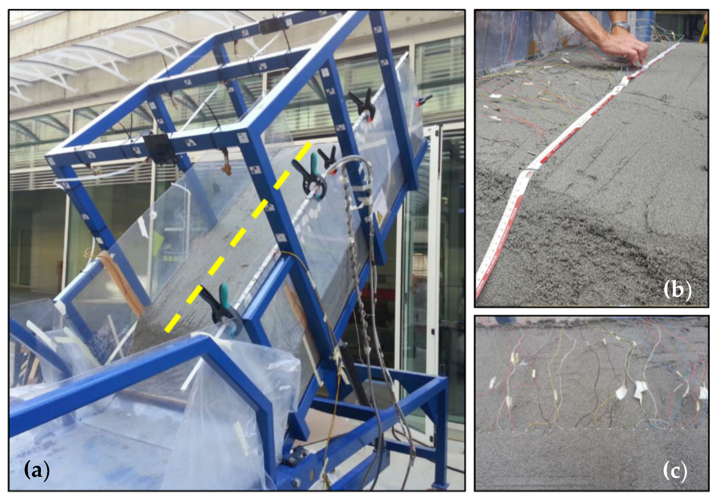
2.1. Experimental Setup

Experimental activities were setup in the laboratory of mountain hydraulics and applied geology situated in the Lecco campus of Politecnico di Milano, Italy. In order to accommodate the simulation of sliding soil masses, a steel structure facility was constructed (Figure 1a). It is composed of two adjustable surfaces [23]. The upper one hosts the terrain under investigation. It has dimensions of 2 m × 0.8 m and its inclination can be raised up to 45°. The lateral sides of the channel are made of Plexiglass for better visual inspection, while the bottom is equipped with a geogrid (TENAX HF geonet made with high density polyethylene/ethylene vinyl acetate HDPE/EVA polymers, angle of friction up to 36° [24]), in order to ensure friction between the soil mass and the structure and avoid the collapse of the soil at a predefined failure surface. The downstream boundary features an oblique finishing (c.a. 30°), with no obstructions to allow for drainage, as any natural slope would likely behave. For what concerns the lateral boundaries, the landslide body was constructed with at least 10:1 ratio of length/depth (0.075 in the present case), in order to minimize the effect of lateral boundaries, congruent with the infinite slope assumptions, typically adopted when carrying out a limit equilibrium analysis. The structure features a sprinkler system designed to simulate rainfall of various intensities. The system consists of 6 sprinklers distributed in two rows by 3 sprinklers running in parallel to the sloping surface (upstream to downstream). The sprinklers supply a spray cone with an angle of 45° over the landslide surface, at a height of 0.6m above. Spray-like discharge nozzles were chosen in order to avoid any erosive action of water droplets. The sprinklers’ distance from the surface and angle of orientation was set in order to supply simulated rainfall in a uniform manner. A set of 20 experiments has been carried out. Most of the experiments (16) featured generic homogeneous sand (d₅₀ = 0.35mm, C_u = 1.75, φ = 34°), while two other mixtures were used for the remaining 4 (see Supplementary Material) containing gravel (C_u = 1.9, d₅₀ = 0.42mm and C_u = 4.7, d₅₀ = 1mm, respectively where C_u = d₆₀/d₁₀ is the uniformity coefficient). Volumetric water content (VWC) of the soil was monitored through a time domain reflectometry (TDR) probe at 1-minute intervals, which was considered a sufficient resolution over the duration of the experiments (24 mins on average (

Table 1. Summary of experimental parameters. The full set of data is available as Supplementary Material.

Value	Rainfall Intensity I [mm/h]	Volume of Water Vw [l]	Porosity n [-]	VWC θ [-]	Degree of Saturation Sr0 [-]	Slope α [deg]	Hydraulic Conductivity ks [m/s]	First Failure tf [min]
Min	48	12	0.44	0.044	0.08	30	4.4 × 10−4	12
Mean	79	40	0.5	0.1	0.34	37.5	6.6 × 10−4	24
Max	122	69	0.54	0.18	0.2	40	1.1 × 10−3	36

)). The probe was placed at mid-depth of the soil, in order to avoid the effects of the highly resistive boundaries at the bottom of the simulator and the air on the surface. The volumetric water content measured by the probe is an average value estimated along the probe length (15 cm). Action cameras were installed on the frame of the simulator [25], in order to document ongoing processes. Images were taken at 2s intervals in order to identify swiftly developing failure processes during the experiment. Rainfall intensity was then estimated through the known relationship of pressure-sprinkler discharge, and the surface area covered by the spray cones.

Soil was placed in the flume in layers with uniform compaction across the channel, that was ensured by fitting a known mass of soil to a certain volume in the channel. The soil samples were compacted using wooden boards, over which weight was applied until a given mass of terrain fitted the predefined volume. The depth of the soil layer was set to 15 cm in all 20 experiments. Initial soil moisture content was set to a predefined value at the beginning of the experiment. After the terrain was settled, the upper platform was lifted to form the desired inclination. Rainfall was then initiated and controlled to maintain a constant value through a pressure control valve. Rainfall was simulated in three different ways. The rainfall pattern followed a constant rainfall in 11 experiments (C-M), or a ‘natural’ pattern with rising and recession limbs, respectively during two of the experiments (A, B). The remaining 7 experiments involved a constant rainfall intensity, followed by a pause, and another constant rainfall, until collapse (N-T). Low intensity rainfall was simulated by using four out of the six sprinklers (experiment M, the first 10 minutes of experiments N, O, P, Q, R), while the higher intensity precipitation involved all of the sprinklers. The hydraulic conductivity of the soil sample was calculated for each of the experiments as a function of its porosity and characteristic grain size, d₁₀ according to the Kozeny–Carman model [26]. A summary of the abovementioned parameters is proposed in Table 1, including the minimum, average and maximum values of rainfall intensity, total volume of water, porosity, volumetric water content, degree of saturation, inclination, hydraulic conductivity and duration until first failure. A detailed description of the experimental parameters is available as Supplementary Material.

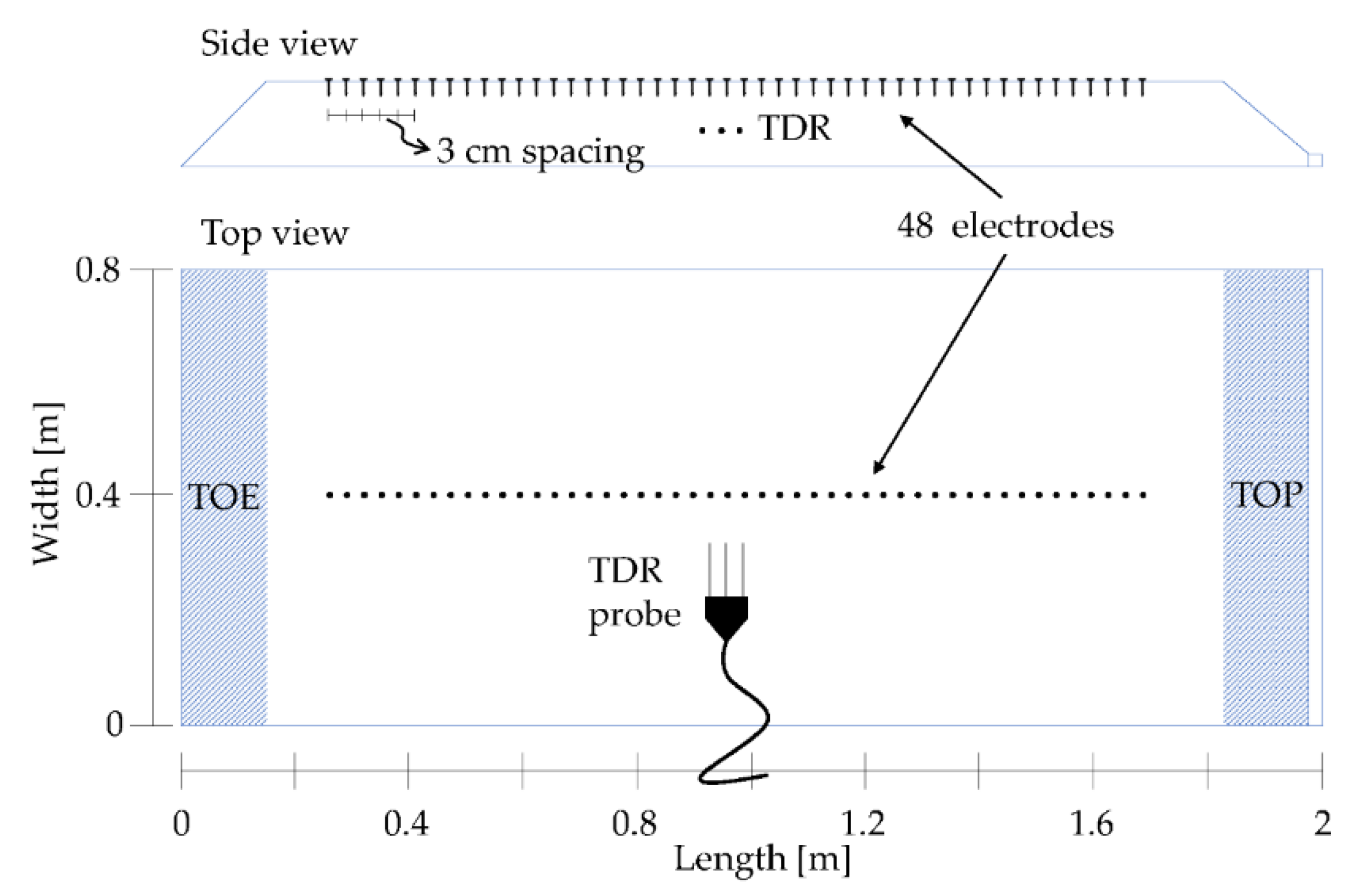
2.2. Geoelectrical Surveys

Geophysical methods have been commonly used to assess the stability of slopes and embankments [27,28,29,30]. In particular, electrical resistivity tomography (ERT) has shown to be efficient in monitoring the variations of water saturation and detecting seepage zones for a variety of studies focused on hydrogeological issues (e.g., [31,32,33,34,35]). In order to obtain a better view of the processes leading to collapse, several experiments featured electrical resistivity tomography (ERT) measurements. To perform time-lapse ERT measurements, two 24-channel mini cables were setup (Figure 1a,b; Figure 2), compatible with the IRIS Syscal Pro geo-resistivitymeter used for the tests. Cables were connected to 48 stainless steel 0.02m-long mini electrodes. A Wenner array with electrode spacing of 0.03m (Figure 2) was used for ERT measurements, resulting in a 1.41m long profile, considered sufficient for the proper analysis of resistivity in the slope. A schematic representation of this configuration is presented in Figure 2. An ERT spread was deployed along the slope axis in all tests, in order to detect resistivity changes along the entire length of the slope and to provide a 2D resistivity image. Mini electrodes were buried at 0.01m depth to prevent preferential infiltration pathways at the locations of the electrodes. A resistivity pseudosection was measured every 3–4 minutes, using the high-speed option of the IRIS Syscal Pro resistivity-meter. This setup allows for the maximum temporal resolution of the measurements in order to obtain a temporally dense record of resistivity changes, and thus, to better monitor the variations of saturation. As a result, we obtained a set of resistivity maps at different instants, which allowed to assess resistivity variations during the experiment that are directly related to soil water content changes. We decided to consider resistivity values instead of water content data, in order to avoid the introduction of uncertainties related to the type of terrain and its effective porosity. Detailed procedures on the choice of the best sampling configuration, corrections for the influence of boundary conditions, and data post-processing can be found in Tresoldi et al. (2019) and Hojat et al. (2019) [34,35].

2.3. Data Analysis

Experimental data were put together and analysed at several steps. The first method applied to the investigation was the Buckingham’s Π theorem [36], applied to the functional relationship between time of failure, predisposing factors and processes leading to the saturation of a given soil sample. This approach allows for the representation of the problem in a dimensionless form, and thus renders possible the comparison of the downscaled simulations to a full-scale problem, and it allows one to take into consideration possible scale effects. This analysis sheds light on the interconnection between the governing variables and allows for the estimation of relative differences originating from changes in temporal and spatial scales. The analysis proposed here with reference to the experimental data, follows the work of Iverson (2015) [22], who proposes a detailed discussion on the importance of carrying out the due dimensional analysis when downscaling land mass failures. While in the aforementioned work, the velocity of debris flow was identified as the dependent variable, we focus on the time of failure, t_f. The dimensional analysis is followed by a principal component analysis (PCA), applied to the experimental observations on some of the previously outlined dimensionless groups. This explorative statistical approach facilitates the quick outline of possible relationships among the participating variables in a dataset of non-negligible dimensions.

2.3.1. Dimensional Analysis

The moment of failure of the landslide body depends on a series of variables and can be framed in the following functional relationship:

$$t_f=f_1\left(\psi , \rho , g, k_s,V_w,H,L,I,i,S_{r0},n,\alpha ,\varphi \right)$$

(1)

where $\psi$ is a generic stress variable describing the state of the pore fluid within the material; $\rho$ is the bulk density of the landslide body mixture; $g$ is the acceleration due to gravity; $k_s$ is the hydraulic conductivity of the landslide body; V_w is the total amount of rainfall water, H and L are the depth and length of the landslide body, respectively; I is the precipitation intensity; i is a term describing the water infiltration rate; $S_{r0}$ is the degree of saturation of the soil at the start of the experiment, n is the soil porosity; $\alpha$ is the inclination of the landslide body; $\varphi$ is the coefficient of internal friction of the material.

According to the Buckingham’s theorem, this functional relationship between n₁ variables comprised of n₂ fundamental dimensions can be expressed as n₁ − n₂ dimensionless groups. The fundamental dimensions pertinent to the problem are mass [M], length [L], and time [T]. The intrinsically dimensionless variables $(S_{r0},n,\alpha ,\varphi$) play no role in the formation of the successive dimensionless groups. Instead, the rest of the quantities can be rendered non-dimensional by using three repeating variables as a base. Here, the triplet $\left(\rho , g, k_s\right)$ is chosen, forming the following dimensional set $\left[\frac{\mathrm{M}}{{\mathrm{L}}^3}, \frac{\mathrm{L}}{{\mathrm{T}}^2},\frac{\mathrm{L}}{\mathrm{T}}\right]$. The choice of repeating variables might be arbitrary and largely dependent on the problem under investigation. In particular, here we considered variables which are pertinent to the physical properties of the soil body ($\rho$), its capacity to convey infiltrating water, ($k_s$) as well as the main force under which failure occurs—gravitational acceleration ($g$). In order to render each of the remaining variables non dimensional, a dimensional homogeneity should be imposed between each term and the repeating variables, all of the latter expressed in terms of their dimensions and raised to unknown powers:

For instance, for $t_f$ we have:

$$\underset{t_f}{\underbrace{{\mathrm{M}}^0{\mathrm{L}}^0{\mathrm{T}}^1}}=\underset{\left(\rho g k_s\right)}{\underbrace{{\left(\frac{\mathrm{M}}{{\mathrm{L}}^3}\right)}^{\mathrm{a}}{\left(\frac{\mathrm{L}}{{\mathrm{T}}^2}\right)}^{\mathrm{b}}{\left(\frac{\mathrm{L}}{\mathrm{T}}\right)}^{\mathrm{c}}}}$$

(2)

Equating the exponents of each of the fundamental dimensions on the left- and right-hand sides, respectively, we have:

$$\{\begin{array}{c}M: 0=a\\ L: 0=-3a+b+c\\ T: 1=-2b-c\end{array}$$

(3)

Which results in a = 0, b = −1, c = 1, and yields the following dimensionless group: $\frac{t_{f}g}{k_s}$.

A similar procedure is applied to the remaining quantities in order to obtain the following dimensionless functional relationship:

$$\underset{{\mathsf{\Pi }}_1}{\underbrace{\frac{t_{f}g}{k_s}}}=f_2\left(\underset{{\mathsf{\Pi }}_2}{\underbrace{\frac{k_s^2}{\mathsf{\psi }}\rho }}, \frac{k_s^2}{\mathrm{gH}} ,\frac{k_s^2}{\mathrm{gL}},\underset{\dots .}{\underbrace{\frac{V_w{g}^3}{k_s^6}}}, \frac{I}{{\mathrm{k}}_s}, \frac{i}{{\mathrm{k}}_s}, S_{r0}, \alpha , n,\underset{{\mathsf{\Pi }}_{11}}{\underbrace{\varphi }}\right)$$

(4)

The dimensionless variables may, however, be somewhat difficult to interpret from a physical point of view. In fact, the non-uniqueness of this analysis indicates that it could be justifiable to revise the dimensionless groups, by combining them through algebraic manipulations motivated by experience and physical insight [22]. For instance, knowing that the characteristic time scale for an object accelerating under the force of gravity is $\sqrt{L/g}$, where L is a length scale and $g$ is the gravitational acceleration, it is reasonable to do the following transformation: ${\mathsf{\Pi }}_1{}^2/{\mathsf{\Pi }}_3$, resulting in ${\mathsf{\Pi }}_1=\frac{t_f}{\sqrt{H/g}}$. Thus, after some manipulations consisting in multiplication and/or the division of dimensionless groups, the above relationship can be rewritten in the following form:

$$\frac{t_f}{\sqrt{H/g}}=f_3\left(\frac{\mathsf{\psi }}{\rho gH}, \frac{{\mathrm{k}}_s}{\sqrt{Hg}},\frac{V_w}{H{k}_s^2/g},\frac{H}{L}, \frac{I}{{\mathrm{k}}_s}, \frac{i}{{\mathrm{k}}_s}, S_{r0}, \alpha , n,\varphi \right)$$

(5)

The construction of a dimensionless relationship permits (1) the exploration of dependencies between the underlying variables and (2) to assess the effects of downsizing/upsizing a given problem. As in this work, we are dealing with a downscaled, or a prototype model of a theoretical existing real scale system, some considerations should be made regarding the quantities involved in the analysis.

Assuming size downscaling of the problem, we will have that $H_2=\gamma H_1$, where $H_1$ and $H_2$ are the depths of the full-scale problem and the prototype, respectively, and $\gamma$ is a scale factor. In order to maintain similarity between the two frameworks, the following equation must hold:

$$\frac{t_{f1}}{\sqrt{H_1/g}}=\frac{t_{f2}}{\sqrt{H_2/g}}$$

(6)

Implying that

$$t_2=t_1\sqrt{\gamma }$$

(7)

Similarly, this relationship applies to the rest of the quantities

$$\frac{k_{s2}}{k_{s1}}=\frac{I_2}{I_1}=\sqrt{ \gamma }$$

(8)

A particular attention should be devoted on $k_s$, the hydraulic conductivity of the soil, as a transition from one scale to another, and a difference in the hydraulic conductivity of the terrain will inevitably imply a difference in the type of material. Empirical relationships relate the hydraulic conductivity of a soil to a characteristic grain diameter, in its simplest form:

$$k_s\propto D_{10}^2$$

(9)

In combination with Equation (8), this relationship implies that

$$D_2=\sqrt[4]{\gamma }{D}_1$$

(10)

This relationship allows one to estimate the correspondence between material used in laboratory conditions and the respective one in a real scale problem and vice versa.

2.3.2. Principal Component Analysis

In order to perform a preliminary explorative analysis on the experimental dataset, a principal component analysis (PCA) was applied. Such an analysis permits the quick identification of relationships among variables in a dataset of moderate dimensions [37]. This statistical tool extracts the best linear lower dimension subset of a multivariate dataset, by reiterating the dataset into a set of factors as linear combinations of the original variables. This is achieved by generating a set of new dimensions, or components, which explain the variations in the data matrix [38]. More particularly, the approach of the PCA is to perform the eigen decomposition of the variables’ covariance matrix. The resulting eigenvectors represent the principal components (or the directions of the new sub space), while the eigenvalues determine their magnitude. Thus, each component is a linear combination of the original variables, where the influence of each variable for the formation of a given component is expressed through the factor loading. The factor loadings are therefore a measure of the correlation between a principle component and the original variables, analogously to the Pearson’s R in regression analysis. In fact, the squared factor loading accounts for the percent of variance in a given variable, explained by the factor. Instead, the representation of the original variables into the newly formed coordinate system is expressed through the factor scores.

The PCA was applied considering the following variables: initial degree of saturation, S_r0, initial volumetric water content, θ soil porosity, n, landslide simulator inclination, α, dimensionless hydraulic conductivity of the material, k_s/(Hg)^0.5, dimensionless rainfall intensity, I/k_s, and the dimensionless volume of rainfall water, V_w/(Hk_s²/g), the dimensionless duration until collapse, t_f/(H/g)^0.5. Twenty observations of the variables are considered, each corresponding to one experiment (Supplementary Material).

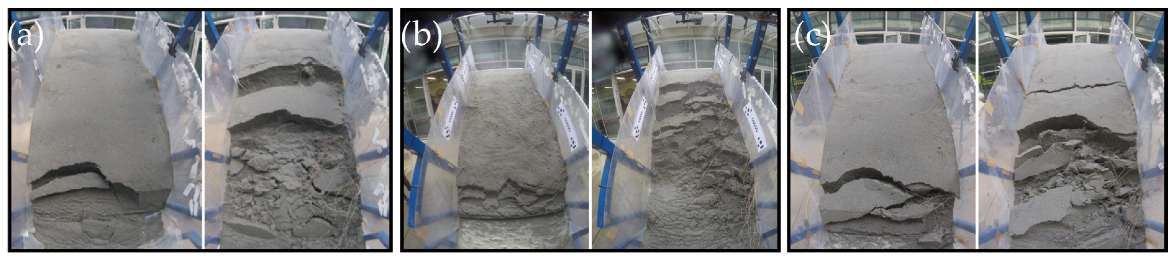
3. Results and Discussion

After sprinkler activation, progressive wetting front propagation eventually led to slope failure, usually after about 25–30 minutes, with some exceptions. Upon destabilization, cracks appeared on the surface of the sand layer and their aperture extended up to a failure. This process developed into a discontinuous failure, where blocks of material detached from the main mass, forming curvilinear sliding surfaces (a visual representation of the process is available in the following subsection). Failure generally started from the lowermost section of the slope and continued in a retrogressive manner towards the top of the flume. However, some experiments featured a crack opening mid-slope, while the upper section of the soil body usually remained less active. Initial failure was preceded by the formation of spring-like outflow observed at the toe of the soil body. The tendency of the lower end of the soil to fail first suggests that the relatively high slope gradients contribute to the swift downhill infiltration of rainfall water. In terms of depth, failure occurred within the soil layer and never on the sand-flume interface, which diminishes the effects of this boundary on the validity of the observations.

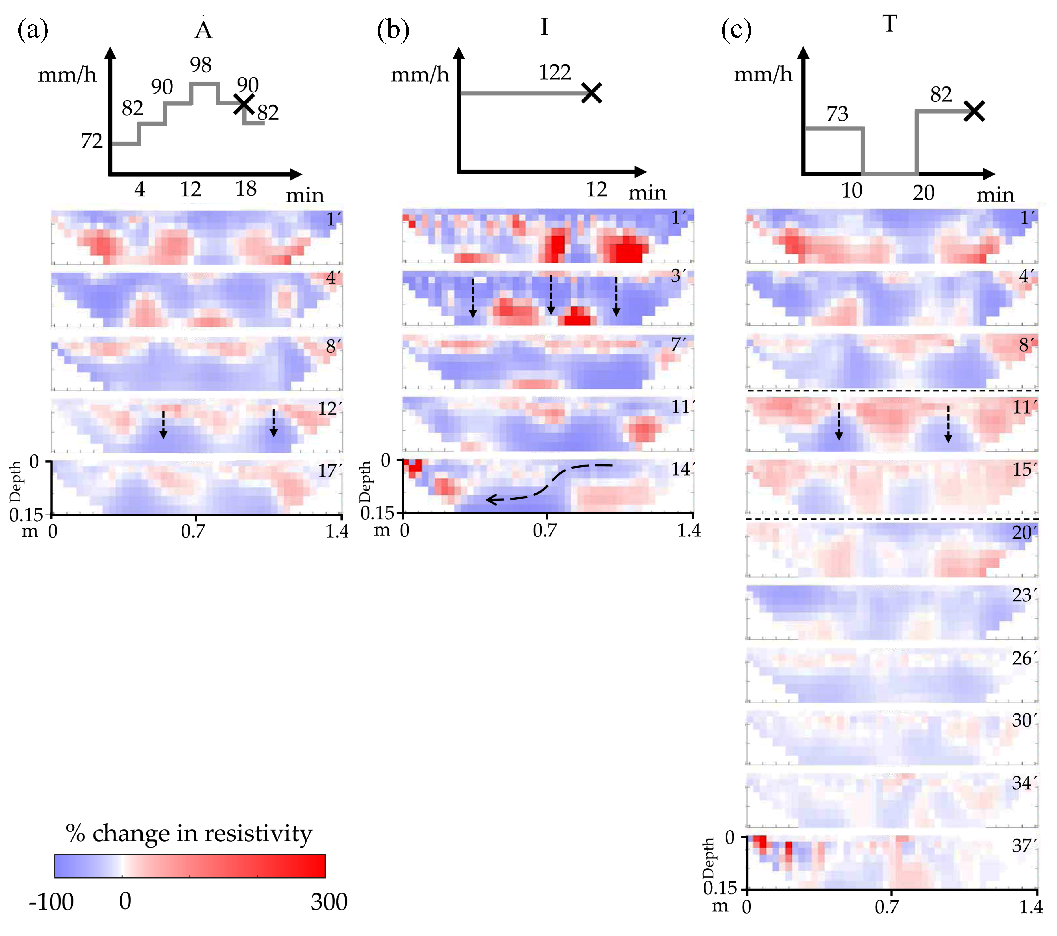
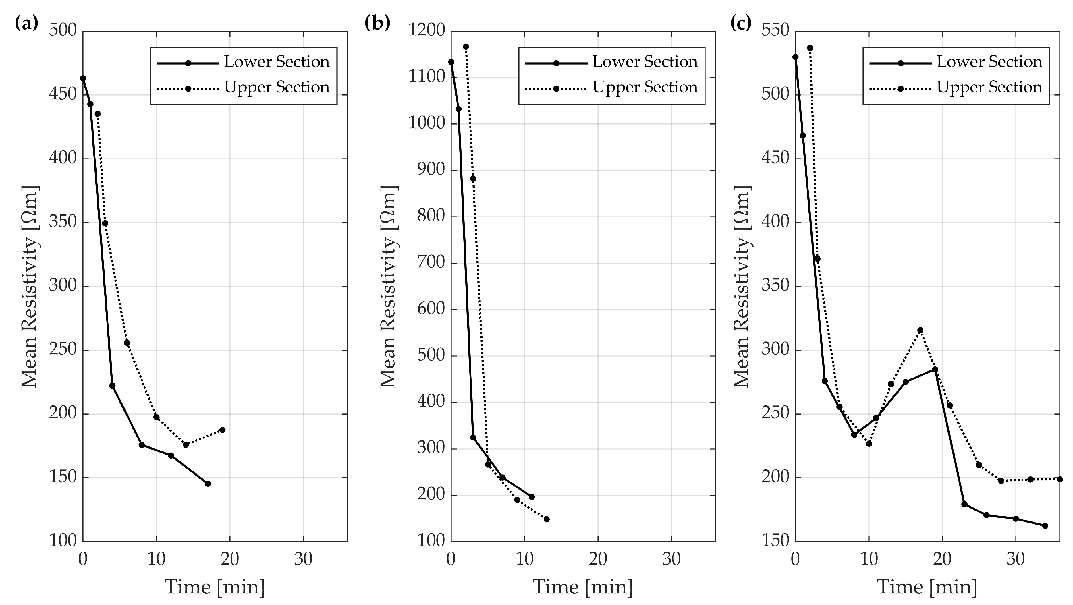
3.1. Geoelectrical Measurements

In order to explore how the waterfront propagates in time in detail, soil resistivity sections have been collected during three of the experiments. Results of the ERT measurements are presented on Figure 3, in terms of relative changes between consecutive resistivity sections. Here we take into account 3 tests, representative of (A) a gradually increasing hyetograph, (I) a constant one, and (T) an experiment featuring a pause, but involving similar volume of rainfall water (see Supplementary material). Increase (decrease) of resistivity is related to the decrease (increase) of water content in the terrain and therefore relative changes account for the infiltration of rainfall water within the landslide body. Measurements were taken at intervals of around 3–4 minutes until slope failure occurred, and thus the electrodes were exposed to the free surface with no ground coupling. Differences in the rainfall water propagation can be observed in each of the cases:

Experiment A simulated the gradual increase of rainfall intensity, in an attempt to represent a realistic shape of the rainfall curve. Propagation of the wetting front was rather quick and caused a sudden collapse, which took place before the complete saturation of the terrain, as demonstrated on Figure 3a.

Looking at Experiment I instead (Figure 3b), it appears that the intensity of rainfall dominates in this case, where an even quicker response of the soil to water infiltration can be observed. It could be argued that the fast development of the process involves a dynamic component in the course of redistribution of stresses, which could be absent during slower infiltration rates. During this process, the gas phase is being expelled from the pores, causing soil matrix deformation, as explained by Lora et al. (2016) [39]. Even though the initial volumetric content in this case is almost half with respect to the rest of the experiments (Supplementary Material), the high intensity rainfall was able to quickly generate instability in the terrain, as depicted by the most pronounced shades of blue on the resistivity change images. In the images collected at t = 14min, we can identify a preferential subsurface flow (arrow in the image). The occurrence of the first fracture is indicated by the red area in the upper left corner of the plot (t = 14min).

Looking at the results from Experiment T (Figure 3c), two infiltration zones can be identified by the consistently blue colour in consecutive images. During the rainfall pause, an increase in resistivity can be observed, as a result of water infiltration in the vertical direction, allowing for air to re-occupy the pore space. It is possible to recognize the water path in the soil mass, with the bottom part more conductive and the shallow layer becoming more resistive, due to the migration of pore water. Instead, after the period of pause, the re-activation of rainfall simulation leads to a more uniform distribution of water content over the entire landslide, with a general decrease of resistivity and some accumulations towards the lower part of the flume, due to its inclination. Steady water infiltration continues and, for the final 7 minutes of the experiment, no significant change was observed. This is interpreted as the near full saturation of the terrain, which ultimately leads to the collapse, evidenced by the fracture aperture at the flume’s toe, illustrated by the red zone in the last image. Areas of concentrated high resistivity near the surface indicate the presence of air associated to the opening of a discontinuity within the soil mass.

Differences in the mode of collapse could also be identified (Figure 4). While Experiments A and T are characterized by an abrupt detachment of chunks of terrain in a retrogressive manner, Experiment I demonstrates a continuous process of soil being liquified and eroded downstream. It is remarkable that, even though the same amount of water has been sprayed on the surface, the drier sample reached such conditions, while in the case of Experiment A, chunks of soil detached as more or less intact portions of sand (Figure 4). Differences in the mode of collapse emerge from the difference in the velocity of wetting front propagation, that is in turn controlled by the rainfall event characteristics, as well as the initial soil moisture content.

In order to track water saturation changes during the tests and to assess how they affect the stability of the slope, we computed mean resistivity values of the lower and upper section of the inverted resistivity maps, corresponding to the lower and upper sections of the slope, respectively. For each test (A, I and T), the curves plotted in Figure 5 display the mean values computed considering all the resistivity maps collected before the appearance of a fracture on the surface of the slope. Although the initial resistivity values of the considered tests are different, in the beginning one can observe a high negative gradient, due to the high permeability of the material and its low initial water content. The rainfall pattern appeared to have a major influence on how water is accumulating within the slope. Consequently, this difference led to the formation of fracturing at the toe of the slope in Tests A and T, while a more distributed sliding was observed in Test I (Figure 5, Supplementary Material).

The decrease in resistivity and corresponding change in soil moisture content indicate the accumulation of water in the lower section of the landslide body during Experiments A and T, with a more prominent effect of this distribution during Experiment T. The intermediate pause during Experiment T is clearly visible through the previously described increase of resistivity values. This is particularly true for the upper section and marks the slope-wise infiltration of pore water towards the lower section. Resistivity values measured during Experiment I illustrate the extremely swift change in water content, despite the low initial values (corresponding to higher resistivity). A negligible difference between the final values measured can be noticed, which indicates a more uniform distribution of the rainfall water in the upper and lower sections. The high rainfall rate here does not allow for a further redistribution and slope-wise infiltration, ultimately leading to a distributed collapse involving a larger portion of the slope.

3.2. Principal Component Analysis

The results of the principal component analysis will be investigated in light of the stability governing process simulated during the experimental tests—the propagation of a wetting front—a process that is strongly affected by the initial state of the soil, as well as the triggering rainfall event.

The analysis outlined three components, accounting for most of the variability in the dataset (85%). The first two components are considered the most relevant for the current analysis. The first principal component can be interpreted as the descriptor of the dynamics of the process, relating initial conditions of the soil, the forcing agent in terms of rainfall intensity and water volume, and the duration until the failure of the landslide. The second principal component is characterized by moderate loadings of initial moisture content followed by a lower contribution of the inclination. Essentially, this component can be interpreted as the initial state of the landslide body. Figure 6 illustrates a biplot containing the factor loadings and factor scores constituting PC1 and PC2 on the x- and y-axis, respectively. High factor loadings are attributed to I/k_s and t_f on PC1, indicating a possible inverse correlation between those variables, implying that higher rainfall intensity leads to a shorter duration until failure. A similar deduction can be captured from the moderate loading of S_r0 on the opposite sides of PC1, with respect to the time of failure, t_f. Although not so pronounced, this relationship indicates that the higher initial water content could be the cause for a faster collapse. Moreover, the analysis indicates a possible positive correlation between the time of failure and the porosity of the material, and in turn its hydraulic conductivity, k_s. The latter trend is, however, likely biased by the relatively high porosity values of the cluster of experiments featuring a pause.

The factor scores relative to the observations and thus labelled with the corresponding letter indicate the similarities between observations (experiments), in terms of the two principal components. A certain clustering of the experiments can be identified on the plot. The left-hand side of Figure 6 contains the experiments with low inclination and an initial degree of saturation. The opposite side of the plot contains experiments characterized by a higher rainfall intensity and shorter duration until failure:

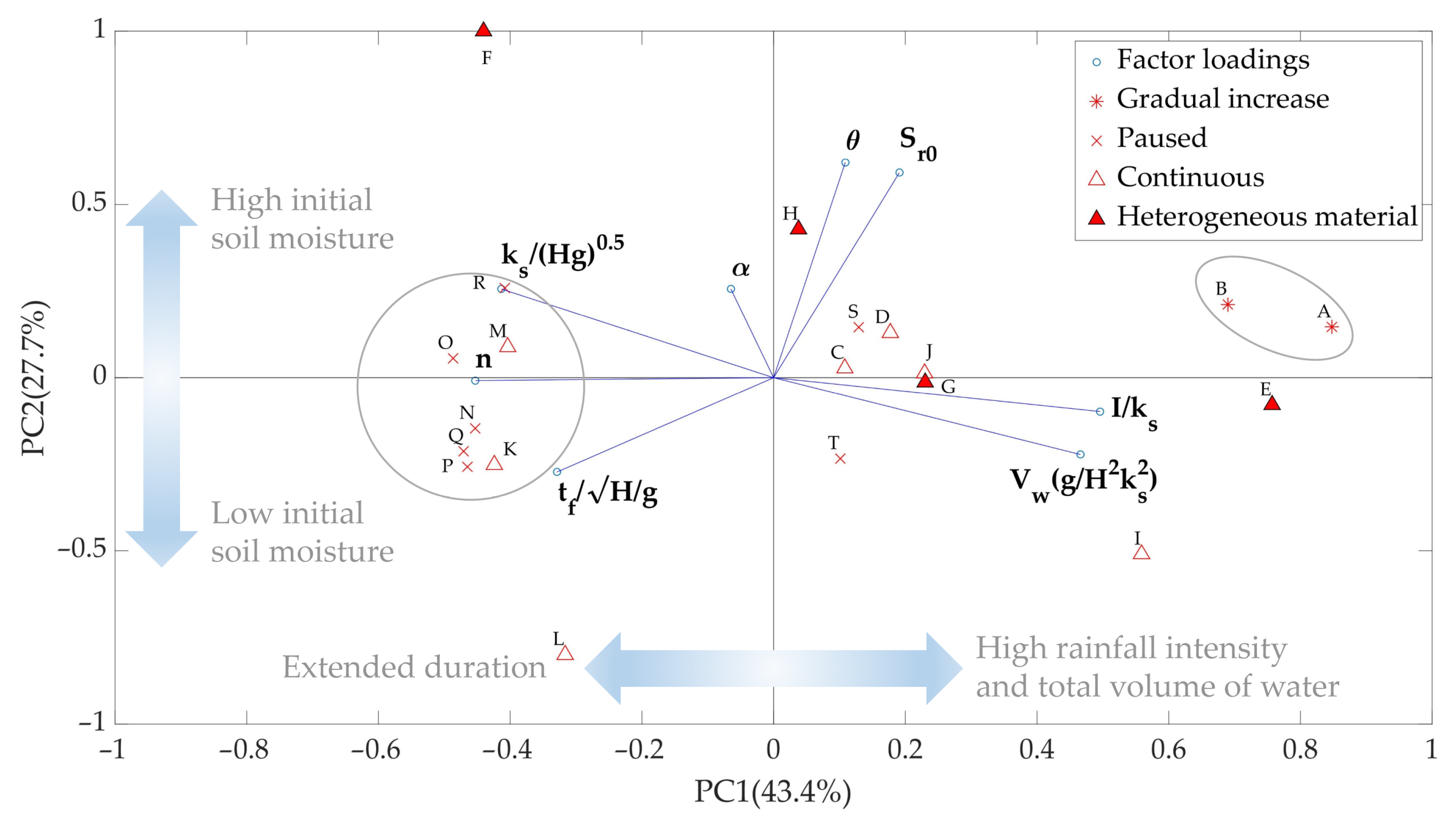
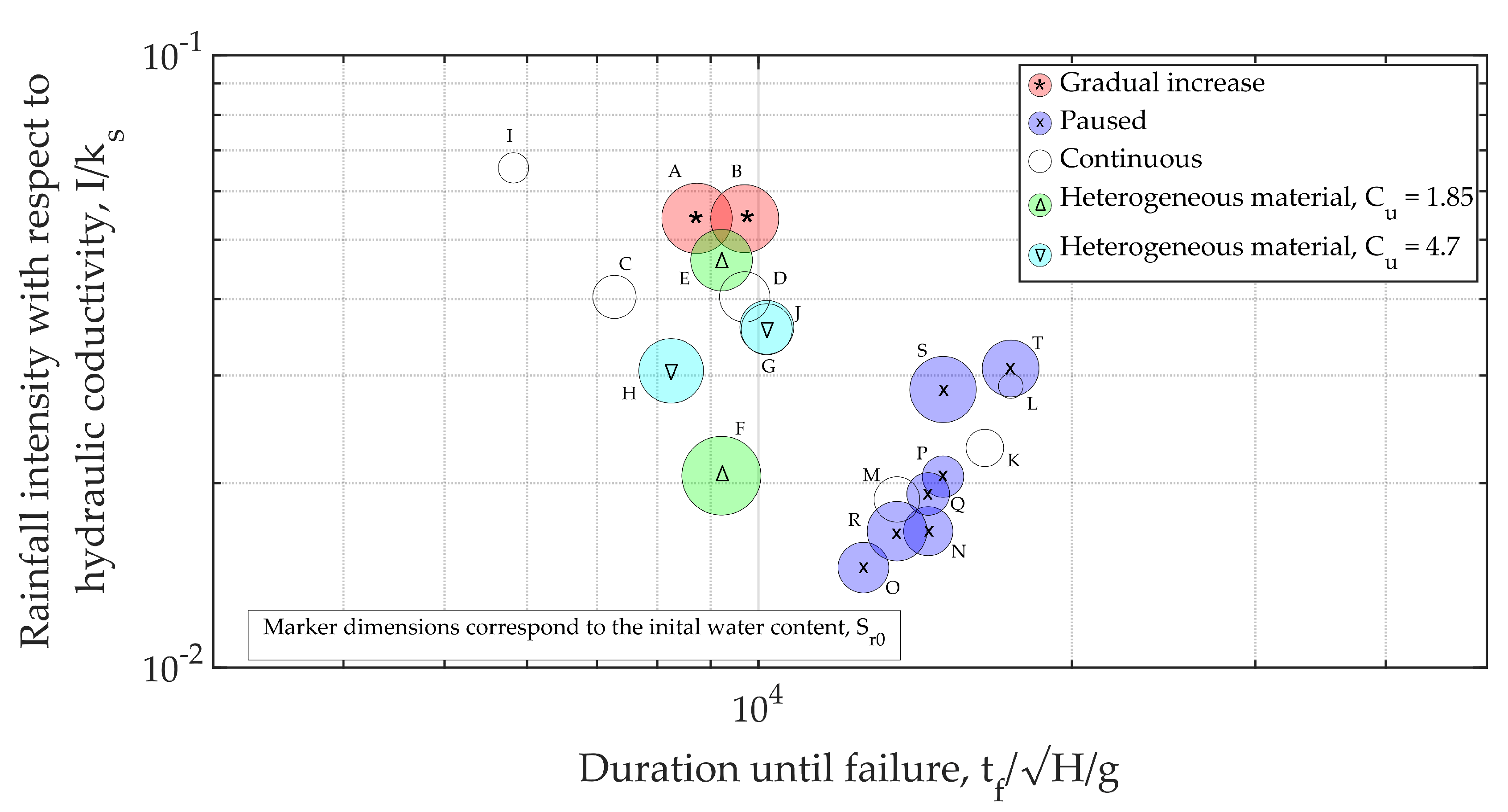
• Experiments which featured a pause tend to cluster together towards the left-hand side of the plot, indicating their higher duration until collapse. Experiments S and T make an exception, as the rainfall intensity during those tests was slightly higher and thus, they deviate from the cluster. Amidst those, the experiment with the lowest rainfall intensity can be found (M), as well as Experiment K, which featured a concentrated rainfall in the upper part of the landslide.
• Experiments with a gradual increase of rainfall simulation cluster together (A, B).
• Experiments with heterogeneous material demonstrate a different behaviour according to the initial state of the soil (E, F, G, H).
• Experiments representing extreme conditions can be outlined as well: Experiment I, characterized by an extremely high precipitation rate, is situated in the lower left corner of the plot, indicating that despite the lower initial soil moisture content, a prompt failure occurred. The experiment with the lowest inclination and initial degree of saturation can be found in the lower left corner of the plot as well (L).

3.3. Parametric Trends

The first and more obvious relationships indicated by the PCA, and subject to further investigation, are the relationship between the dimensionless duration until failure, the dimensionless precipitation intensity, and the initial degree of saturation of the soil. Figure 7 illustrates the experimental data in different colours according to the distinct features of the experiments, while the dimension of the marker reflects the value of initial degree of saturation. A decreasing trend can be identified in the experimental data, likely a nonlinear one. This outlines the range of events which bring the slope to failure—from high intensity and short duration, to a lower intensity combined with a longer duration. This relationship is however influenced by the initial state of soil moisture, indicating that events with higher initial soil moisture could lead to failure at lower rainfall intensity. The clustering of datapoints can be observed, which corresponds to the results obtained from the PCA.

An evident shift of the experiments featuring an intermediate interruption towards the right-hand side of the plot marks the longer duration of those with respect to the rest of the observations. This cluster also includes Experiments K and L, which did not feature a pause. The initial soil moisture of those two cases is, however, rather reduced, while rainfall intensity here is low, which explains this deviation. Moreover, during Experiment K, a concentration of rainfall was simulated in the upper portion of the channel, which suggest that the process of wetting front propagation here is different in what just a portion of the slope is affected by rainfall.

Observations of Experiment I indicate its quite swift collapse. It is worth noting here that, despite the low initial soil moisture, the high rainfall intensity developed instability, indicating that, in this case, the stability of the slope was entirely governed by the rapid wetting front propagation. Instead, if one is to interpret the simulations involving a pause as series of rainfall events, the importance to consider antecedent hydrological and hydrogeological conditions is clearly brought forward. More particularly, this can be interpreted as the effect of “internal damage” within the soil layer, gradually affecting the mechanical status of a hillslope and undermining its successive ability to remain intact during future events [7]. Modification of the granulometric distribution of the soil with a portion of a more coarse material (Cu = 1.85 and Cu = 4.7), ultimately representing a higher capacity of the soil to convey the rainfall water, does not demonstrate any particular effect, if not in the cases in which soil moisture content assumes higher values (F, H). The initial state of the soil appears to govern the process in this case, as it is in fact also the case of Experiments S and T, where the high initial soil moisture combined with the relatively high intensity of rainfall distinguish those experiments from the blue clusters. A provisional division can be outlined, considering the transition from a lower to a higher initial soil moisture content, which renders the destabilization process rainfall intensity-controlled or initial condition-controlled, respectively.

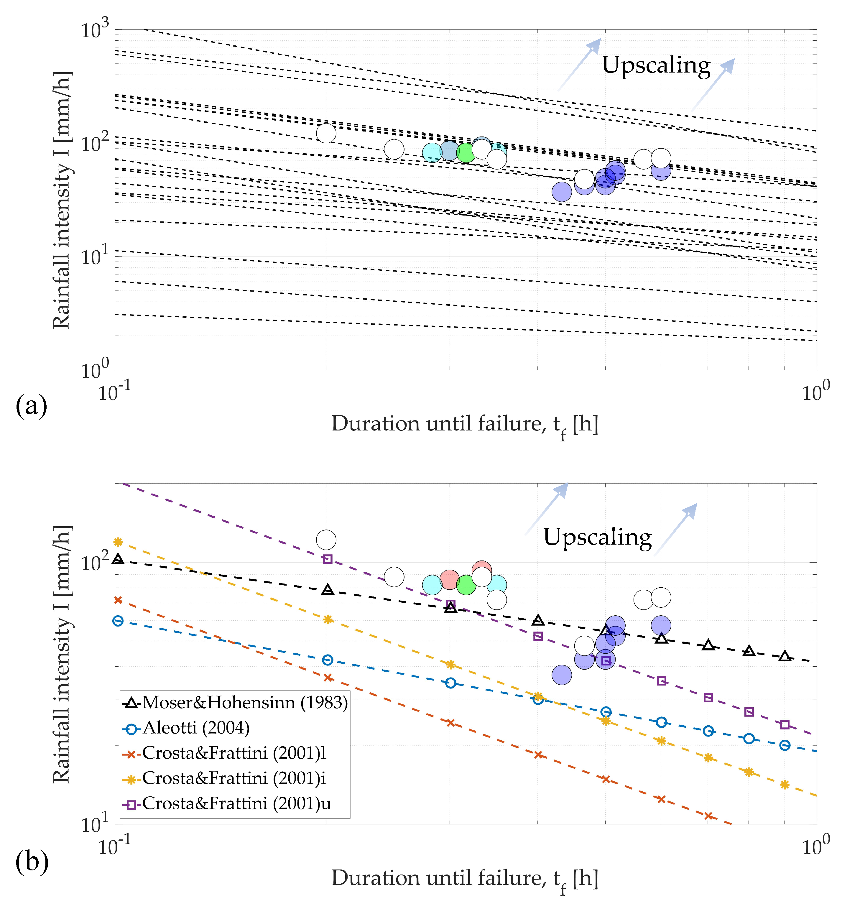
3.4. Rainfall Thresholds

The experimental data were tentatively put in the context of rainfall threshold definition. In general terms, rainfall thresholds are defined by delineating datapoints of rainfall intensity and duration, which led to the occurrence of a landslide. A variety of thresholds exist according to the scale of the problem, which in turn involves different climatic zones, geological contexts, and the typology of shallow landslides including soil slips and debris flows as well [8]. Figure 8a includes the thresholds defined for shallow landslides, listed in the work of Guzzetti et al. (2007) [40]. A great deal of variability of thresholds can be noted. The experimental dataset falls into the range of thresholds, and datapoints are correctly identified as failures by most of the thresholds.

The comparison illustrated here refers strictly to the simulation of the 15 cm depth soil layer. In order to migrate into a full-scale problem, an upscaling can be carried out according to the Buckingham’s Π theorem, considering an increase in the dimensions of the landslide body. This would translate the datapoints far into the so-called critical zone, above the threshold line, due to the quite high rainfall intensity values, which would further increase if an upscaling is performed. Clearly, the results presented here are valid in the domain of laboratory scale experiments, which only mimic a full-scale problem and neglect some full-scale effects, as discussed by Iverson (2015) [22]. The simplification of the problem, however, provides good grounds for the isolation of the most influential processes leading to the failure of a shallow soil mass. In particular, the use of a homogeneous soil in the initial experiments in this work aims to dismiss any effect of possible heterogeneity, and focus on the rainfall infiltration and further distribution of water within the soil. This has been later built up with the addition of material characterized by larger grain size distribution in some of the tests, which demonstrated a different behaviour indeed.

A selection of the thresholds has been chosen according to the type of landslide and type of material involved (Figure 8b). Thresholds defined on shallow landslides composed of mostly non frictional or weak cohesive materials [43], incoherent deposits, debris and loose soil [42], or slightly cohesive colluvial material [41], tend to be a good fit to the data, since they delineate a lower bound that is, at the same time, not too conservative. In particular, the three thresholds defined by [43] tend to fit the dataset in both its trend and the lower bound on the point cloud. The upper threshold of Crosta and Frattini (2001) [43], devised to interpret the maximum intensity events in their dataset, represents a good fit to the cases with high rainfall intensity also in the present case. Instead, the thresholds defined by Moser and Hohensinn (1983) and Aletotti (2004) [41,42] are characterized by a milder gradient. The former encompasses all data points, although with a broad margin, which is most likely due to the threshold being created on the basis of the dataset including debris flows which could be characterized by a different triggering mechanism. The threshold proposed by Moser and Hohensinn (1983) [41] does not encompass the experiments which involved an intermediate pause, situated below the relative threshold line, while the rest are located in the ‘failure zone’. The definition of rainfall thresholds is often characterized by a certain deal of uncertainty, relative to the dataset of landslide-provoking events. On the other hand, the experimental environment offers the possibility to control a set of parameters and therefore, validity of thresholds could be tested under a variety of event scenarios, types of material or event exceptional conditions, such as, e.g., terrains that have undergone a modification of their infiltration properties [44].

3.5. Scale Effects

The dimensional analysis presented in this work has a three-fold interpretation.

• The resulting scale relationships between parameters demonstrate the intrinsic interconnection or “chain” that relates variables. Thus, decreasing the dimensions of the landslide would inevitably have an effect on all other variables.
• This relation could be directly proportional to the scale factor or follow a different degree of proportionality. Hence, downscaling a real event should be carried out with care, as time scales differ from spatial scales for a land mass failure problem, leading to:
• Simulations carried out with soil samples collected from a real case study, and reproducing its triggering rainfall event, could lead to a misinterpretation, if the proper scales are not taken into account.

Since the results presented here do not refer to a specific landslide event, we propose the reciprocal case of upscaling them. Upscaling could yield an indication of the timing required for a slope to fail, or at least its expected order of magnitude. Upscaling geometrically would inevitably involve the corresponding modification in characteristic grain size diameter and thus hydraulic conductivity of the terrain, which in turn, would correspond to a different characteristic grain size. For instance, an increase in the H/L ratio by a factor of ten would increase failure time by $\sqrt{10}$, or roughly 3 times, while the corresponding material would increase by roughly 1.8, following the explanation in Section 2.3.1. Naturally, the rainfall intensity would increase by the same factor as well, leading to an exaggeration of the values in terms of a real rainfall event.

3.6. Summary

The experimental data bring forward two main effects, relative to the complex interaction between shallow landslide triggering event and predisposing conditions. First and foremost, the ratio of the rainfall rate and the ability of the soil to convey rainfall water for a given duration, I/k_s, is a proper descriptor of land mass failure. Secondly, this relationship could be undermined by the preceding soil moisture state, as well as the type of terrain. The former is evident from the simulation of a succession of rainfall events. During the pause period, rainfall water is able to settle down within the terrain and diminish its integrity, which in turn renders the second episode crucial for the stability of the slope event at low I/k_s values. When a full-scale problem is concerned, this effect can be translated into a scenario featuring the succession of rainfall events, which would undoubtedly have an effect on the hillslope behaviour. Under similar initial moisture conditions and with similar amounts of rainfall water, the rates of precipitation appear to control stability. Higher rainfall rates could bring down the slope to failure much faster under similar initial conditions (e.g., Experiment I vs. Experiments K, L in Figure 7). This appears to be valid both for constant rainfall events and gradually increasing ones. The initial degree of saturation however further affects this equilibrium. In fact, very low or very high values or initial moisture content both lead to the rather fast development of instabilities. In the first case, this could be explained by the high rate fluxes of infiltrating water, leading to air exhaust and deformation of the soil matrix, while in the second case, the excessive presence of water renders the bonds between particles intrinsically unstable. Thus, the control over instability could migrate from one parameter to the other in different scenarios.

The results obtained here on a relatively loose cohesionless material would certainly be altered, should the landslide be composed of soil or rock-soil mixture with different characteristics in terms of grain size and compaction and therefore, hydraulic conductivity. The change in hydraulic conductivity of the material would thus alter the ratio I/k_s and, as a consequence, the time required for the slope to reach instability. While the failure mechanism of weakly consolidated granular material would be largely defined by the advancement of a swiftly propagating front, fine-grained cohesive materials would respond with a much different behaviour to a similar triggering event. Apart from the much lower propensity of the soil to water infiltration, cohesion should be considered as well. This would likely lead to an extended failure time and likely a different failure mechanism involving plastic deformations. Some uncertainty in the obtained results could be attributed to the preparation of the experimental setup and more particularly to differences in compaction across the soil sample, even though no peculiarities were observed during the experimental tests. A practice to sample soil material from a given case study and carry out downsized simulations exists throughout the literature. However, this practice would imply dimensional analysis to be applied and the proper scaling of governing variables, in order to ensure similarity between the two domains.

4. Conclusions

In this work, we presented the experimental results of a set of downsized simulations of shallow land mass failures. The simplification of the problem under laboratory conditions allowed emphasis to be put on the key instability drivers, recognized as the triggering phenomenon and the hydrogeological conditions of the slope. A detailed look on the temporal evolution of the failure process was achieved through ERT measurements during some of the experiments featuring different hyetographs. The problem was first approached with a dimensional analysis through the application of the Buckingham’s Π theorem, which acts as a bridge between the experimental tests presented here and their potential implications in a full-scale problem. A preliminary screening of the variables involved was carried out through a principal component analysis, which indicated potential trends in the dataset. Furthermore, the resulting dimensionless groups facilitated the analysis of parametric trends governing the problem. Finally, a tentative comparison with existing rainfall intensity duration thresholds demonstrated that the simulated events are correctly identified as failures by most of the listed thresholds, and specifically by those defined on landslide cases involving non-cohesive or loose material.

The results obtained in this work illustrated the multifaceted role of water for the stability of shallow land masses. The dynamics of wetting front propagation were defined by the complex interaction between rainfall intensity, the ability of the soil to convey the infiltrating water and the antecedent moisture conditions of the soil, where the main control parameter depends on the state of the others. The outcomes of this work suggest that:

• the coupled interaction between rainfall intensity, hydraulic conductivity and soil moisture gradient is governing the stability of soil, and while rainfall intensity and duration are essential instability predictors, they must be integrated with antecedent moisture and site-specific soil property information;
• The above consideration partially explains the great variability of rainfall thresholds for shallow landslide stability found throughout the literature;
• The dynamics of the hydrologic event plays an important role for the advancement of the wetting front and further development of instability, evidenced by the differences outlined during ERT measurement;
• succession of rainfall events predisposes the terrain to failure—a scenario which can be easily translated into large-scale phenomena. The observation of a single hydrological event is therefore insufficient in terms of stability definition;
• the comparison of the dataset with a list of rainfall intensity-duration thresholds suggests that downscaled simulations could potentially be employed for the validation of rainfall thresholds.

The simplified experiments presented here are intended to serve as a preliminary investigation into the effect rainfall water has on the stability of shallow landslides. Inference of those results on a full-scale phenomenon can be obtained by means of a proper upscaling according to Buckingham’s theorem, while implications of such findings can be found into the definition and validation of rainfall thresholds and stability models, as well as the generation of shallow landslide susceptibility and risk maps.

References

1. Hungr, O.; Leroueil, S.; Picarelli, L. The Varnes classification of landslide types, an update. Landslides 2013, 11, 167–194. [Google Scholar] [CrossRef]
2. Lee, D.-H.; Lai, M.-H.; Wu, J.-H.; Chi, Y.-Y.; Ko, W.-T.; Lee, B.-L. Slope management criteria for Alishan Highway based on database of heavy rainfall-induced slope failures. Eng. Geol. 2013, 162, 97–107. [Google Scholar] [CrossRef]
3. Gabet, E.J.; Mudd, S. The mobilization of debris flows from shallow landslides. Geomorphology 2006, 74, 207–218. [Google Scholar] [CrossRef]
4. Radice, A.; Longoni, L.; Papini, M.; Brambilla, D.; Ivanov, V. Generation of a Design Flood-Event Scenario for a Mountain River with Intense Sediment Transport. Water 2016, 8, 597. [Google Scholar] [CrossRef] [Green Version]
5. Papini, M.; Ivanov, V.; Brambilla, D.; Arosio, D.; Longoni, L. Monitoring bedload sediment transport in a pre-Alpine river: An experimental method. Rend. Online 2017, 43, 57–63. [Google Scholar] [CrossRef]
6. Baum, R.; Godt, J.W.; Savage, W.Z. Estimating the timing and location of shallow rainfall-induced landslides using a model for transient, unsaturated infiltration. J. Geophys. Res. Space Phys. 2010, 115, 115. [Google Scholar] [CrossRef]
7. Fan, L.; Lehmann, P.; Or, D. Effects of hydromechanical loading history and antecedent soil mechanical damage on shallow landslide triggering. J. Geophys. Res. Earth Surf. 2015, 120, 1990–2015. [Google Scholar] [CrossRef]
8. Borja, R.I.; Liu, X.; White, J.A. Multiphysics hillslope processes triggering landslides. Acta Geotech. 2012, 7, 261–269. [Google Scholar] [CrossRef]
9. Segoni, S.; Piciullo, L.; Gariano, S.L. A review of the recent literature on rainfall thresholds for landslide occurrence. Landslides 2018, 15, 1483–1501. [Google Scholar] [CrossRef]
10. Guzzetti, F.; Peruccacci, S.; Rossi, M.; Stark, C. The rainfall intensity–duration control of shallow landslides and debris flows: An update. Landslides 2007, 5, 3–17. [Google Scholar] [CrossRef]
11. Lazzari, M.; Piccarreta, M.; Manfreda, S. The role of antecedent soil moisture conditions on rainfall-triggered shallow landslides. Nat. Hazards Earth Syst. Sci. Discuss. 2018, 1–11. Available online: https://www.nat-hazards-earth-syst-sci-discuss.net/nhess-2018-371/nhess-2018-371.pdf (accessed on 22 April 2020). [CrossRef] [Green Version]
12. Tiranti, D.; Nicolò, G.; Gaeta, A.R. Shallow landslides predisposing and triggering factors in developing a regional early warning system. Landslides 2018, 16, 235–251. [Google Scholar] [CrossRef]
13. Zhao, B.; Dai, Q.; Han, D.; Dai, H.; Mao, J.; Zhuo, L. Antecedent wetness and rainfall information in landslide threshold definition. Hydrol. Earth Syst. Sci. Discuss. 2019, 1–26. Available online: https://www.hydrol-earth-syst-sci-discuss.net/hess-2019-150/hess-2019-150.pdf (accessed on 22 April 2020). [CrossRef]
14. Thomas, M.A.; Mirus, B.; Collins, B.D. Identifying Physics-Based Thresholds for Rainfall-Induced Landsliding. Geophys. Res. Lett. 2018, 45, 9651–9661. [Google Scholar] [CrossRef]
15. Iverson, R.M. Landslide triggering by rain infiltration. Water Resour. Res. 2000, 36, 1897–1910. [Google Scholar] [CrossRef] [Green Version]
16. Montrasio, L.; Schilirò, L.; Terrone, A. Physical and numerical modelling of shallow landslides. Landslides 2015, 13, 873–883. [Google Scholar] [CrossRef]
17. Schenato, L.; Palmieri, L.; Camporese, M.; Bersan, S.; Cola, S.; Pasuto, A.; Galtarossa, A.; Salandin, P.; Simonini, P. Distributed optical fibre sensing for early detection of shallow landslides triggering. Sci. Rep. 2017, 7, 14686. [Google Scholar] [CrossRef]
18. Schilirò, L.; Djueyep, G.P.; Esposito, C.; Mugnozza, G.S. The Role of Initial Soil Conditions in Shallow Landslide Triggering: Insights from Physically Based Approaches. Geofluids 2019, 2019, 1–14. [Google Scholar] [CrossRef] [Green Version]
19. Moriwaki, H.; Inokuchi, T.; Hattanji, T.; Sassa, K.; Ochiai, H.; Wang, G. Failure processes in a full-scale landslide experiment using a rainfall simulator. Landslides 2004, 1, 277–288. [Google Scholar] [CrossRef]
20. Michlmayr, G.; Chalari, A.; Clarke, A.; Or, D. Fiber-optic high-resolution acoustic emission (AE) monitoring of slope failure. Landslides 2016, 14, 1139–1146. [Google Scholar] [CrossRef]
21. Papini, M.; Ivanov, V.I.; Brambilla, D.; Ferrario, M.; Brunero, M.; Cazzulani, G.; Longoni, L. First steps for the development of an optical fibre strain sesnor for shallow landslide stability monitoring through laboratory experiments. In Applied Geology: Approaches to Future Resource Management; De Maio, M., Tiwari, A.K., Eds.; Springer: Berlin, Germany, 2020; in press. [Google Scholar]
22. Iverson, R.M. Scaling and design of landslide and debris-flow experiments. Geomorphology 2015, 244, 9–20. [Google Scholar] [CrossRef]
23. Arosio, D.; Hojat, A.; Ivanov, V.; Loke, M.; Longoni, L.; Papini, M.; Tresoldi, G.; Zanzi, L. A Laboratory Experience to Assess the 3D Effects on 2D ERT Monitoring of River Levees. In Proceedings of the 24th European Meeting of Environmental and Engineering Geophysics, Porto, Portugal, 9–12 September 2018. [Google Scholar] [CrossRef]
24. Tenax Geosynthetics. Tenax HF-HF PLUS Technical Data Sheet. Available online: https://www.tenax.net/wp-content/uploads/2017/11/Scheda_Tecnica_TENAX_HF-HF-Plus_i.pdf (accessed on 22 April 2020).
25. Scaioni, M.; Crippa, J.; Yordanov, V.; Longoni, L.; Ivanov, V.; Papini, M. Some tools to support teaching photogrammetry for slope stability assessment and monitoring. Int. Arch. Photogramm. Remote Sens. Spatial Inf. Sci. 2018, 453–460. [Google Scholar] [CrossRef] [Green Version]
26. Wang, J.-P.; François, B.; Lambert, P. Equations for hydraulic conductivity estimation from particle size distribution: A dimensional analysis. Water Resour. Res. 2017, 53, 8127–8134. [Google Scholar] [CrossRef]
27. Wu, J.-H.; Lin, H.-M.; Lee, D.-H.; Fang, S.-C. Integrity assessment of rock mass behind the shotcreted slope using thermography. Eng. Geol. 2005, 80, 164–173. [Google Scholar] [CrossRef]
28. Chambers, J.; Gunn, D.; Wilkinson, P.; Meldrum, P.; Haslam, E.; Holyoake, S.; Kirkham, M.; Kuras, O.; Merritt, A.; Wragg, J. 4D electrical resistivity tomography monitoring of soil moisture dynamics in an operational railway embankment. Near Surf. Geophys. 2012, 12, 61–72. [Google Scholar] [CrossRef] [Green Version]
29. Lai, S.-L.; Lee, D.-H.; Wu, J.-H.; Dong, Y.-M. Detecting the cracks and seepage line associated with an earthquake in an earth dam using the nondestructive testing technologies. J. Chin. Inst. Eng. 2013, 37, 428–437. [Google Scholar] [CrossRef]
30. Zhang, Z.; Arosio, D.; Hojat, A.; Taruselli, M.; Zanzi, L. Construction of a 3D velocity model for microseismic event location on a monitored rock slope. In Proceedings of the EAGE-GSM 2nd Asia Pacific Meeting on Near Surface Geoscience and Engineering, Kuala Lumpur, Malaysia, 24–25 April 2019; pp. 1–5. [Google Scholar] [CrossRef]
31. Nasab, S.K.; Hojat, A.; Kamkar-Rouhani, A.; Javar, H.A.; Maknooni, S. Successful Use of Geoelectrical Surveys in Area 3 of the Gol-e-Gohar Iron Ore Mine, Iran. Mine Water Environ. 2011, 30, 208–215. [Google Scholar] [CrossRef]
32. Supper, R.; Ottowitz, D.; Jochum, B.; Kim, J.-H.; Römer, A.; Baroň, I.; Pfeiler, S.; Lovisolo, M.; Gruber, S.; Vecchiotti, F. Geoelectrical monitoring: An innovative method to supplement landslide surveillance and early warning. Near Surf. Geophys. 2013, 12, 133–150. [Google Scholar] [CrossRef] [Green Version]
33. Arosio, D.; Munda, S.; Tresoldi, G.; Papini, M.; Longoni, L.; Zanzi, L. A customized resistivity system for monitoring saturation and seepage in earthen levees: Installation and validation. Open Geosci. 2017, 9, 457–467. [Google Scholar] [CrossRef]
34. Tresoldi, G.; Arosio, D.; Hojat, A.; Longoni, L.; Papini, M.; Zanzi, L. Long-term hydrogeophysical monitoring of the internal conditions of river levees. Eng. Geol. 2019, 259, 105139. [Google Scholar] [CrossRef]
35. Hojat, A.; Arosio, D.; Ivanov, V.I.; Longoni, L.; Papini, M.; Scaioni, M.; Tresoldi, G.; Zanzi, L. Geoelectrical characterization and monitoring of slopes on a rainfall-triggered landslide simulator. J. Appl. Geophys. 2019, 170, 103844. [Google Scholar] [CrossRef]
36. Bridgman, P.W. Dimensional Analysis; Yale University Press: New Haven, CT, USA, 1922. [Google Scholar]
37. Jolliffe, I.T. Principal Component Analysis, 2nd ed.; Springer: New York, NY, USA, 2002; p. 29. [Google Scholar]
38. Pempkowiak, J.; Beldowski, J.; Pazdro, K.; Staniszewski, A.; Zaborska, A.; Leipe, T.; Emeis, K. Factors influencing fluffy layer suspended matter (FLSM) properties in the Odra River—Pomeranian Bay—Arkona Deep System (Baltic Sea) as derived by principal components analysis (PCA), and cluster analysis (CA). Hydrol. Earth Syst. Sci. 2005, 9, 67–80. [Google Scholar] [CrossRef]
39. Lora, M.; Camporese, M.; Troch, P.A.; Salandin, P. Rainfall-triggered shallow landslides: Infiltration dynamics in a physical hillslope model. Hydrol. Process. 2016, 30, 3239–3251. [Google Scholar] [CrossRef]
40. Guzzetti, F.; Peruccacci, S.; Rossi, M.; Stark, C.P. Rainfall thresholds for the initiation of landslides in central and southern Europe. Theor. Appl. Clim. 2007, 98, 239–267. [Google Scholar] [CrossRef]
41. Moser, M.; Hohensinn, F. Geotechnical aspects of soil slips in Alpine regions. Eng. Geol. 1983, 19, 185–211. [Google Scholar] [CrossRef]
42. Aleotti, P. A warning system for rainfall-induced shallow failures. Eng. Geol. 2004, 73, 247–265. [Google Scholar] [CrossRef]
43. Crosta, G.B.; Frattini, P. Rainfall thresholds for triggering soil slips and debris flow. In Proceedings of the 2nd EGS Plinius Conference on Mediterranean Storms, Siena, Italy, 16–18 October 2001; Volume 1, pp. 463–487. [Google Scholar]
44. Abbate, A.; Longoni, L.; Ivanov, V.; Papini, M. Wildfire Impacts on Slope Stability Triggering in Mountain Areas. Geosciences 2019, 9, 417. [Google Scholar] [CrossRef] [Green Version]
Figure 1. (a) Landslide simulator in a test configuration. Dashed line corresponds to the line of the ERT profile. (b) Electrodes’ insertion along the longitudinal profile of the channel during preparation phase. (c) Close-up image of the electrodes.
Water 12 01203 g001
Figure 2. Schematic representation of the experimental setup in both side and top views.
Water 12 01203 g002
Figure 3. Hyetographs and images representing relative changes between consecutive resistivity sections collected during tests (a) A, (b) I, and (c) T. Dashed lines enclose rainfall pause period. Nil values of the x-axis correspond to the toe of the slope. Numbers in the top right corner of each image indicate the instant (min) in which the measurement was obtained.
Water 12 01203 g003
Figure 4. Mode of collapse of Experiments (a) A, (b) I and (c) T.
Water 12 01203 g004
Figure 5. Mean resistivity values for the lower and upper sections of the slope obtained from the ERT surveys performed in (a) test A, (b) test I, and (c) test T. Lower and upper section resistivity points are delayed in time considering the time taken by the georesistivimeter to scan the entire deployment multi-electrode array (starting from the toe of the slope).
Water 12 01203 g005
Figure 6. A biplot as a result of the principal component analysis. Bold symbols represent the factor loadings on the respective principal components 1 and 2. Symbols A-T represent the factor scores of each of the observations.
Water 12 01203 g006
Figure 7. Dimensionless duration against dimensionless rainfall intensity. The dimensions of the markers represent the initial soil moisture content.
Water 12 01203 g007
Figure 8. (a) Rainfall intensity—duration thresholds for shallow landslide occurrence listed in the work of Guzzetti et al. 2007 [40]. (b) rainfall intensity-duration thresholds defined on the basis of landslide events which involved slightly cohesive or loose material (Moser and Hohensinn (1983) [41]; Aleotti (2004) [42]; Crosta and Frattini (2001) [43] l—lower; i—intermediate; u—upper). Arrows illustrate the effect of upscaling on the position of the datapoints relative to the rainfall thresholds.
Water 12 01203 g008