An Experimental Assessment of Extreme Wave Evaluation by Integrating Model and Wave Buoy Data

Abstract

Calculating the significant wave height (SWH) in a given location as a function of the return time is an essential tool of coastal and ocean engineering; such a calculation can be carried out by making use of the now widely available weather and wave model chains, which often lead to underestimating the results, or by means of in situ experimental data (mostly, wave buoys), which are only available in a limited number of sites. A procedure is hereby tested whereby the curves of extreme SWH as a function of the return time deriving from model data are integrated with the similar curves computed from buoy data. A considerable improvement in accuracy is gained by making use of this integrated procedure in all locations where buoy data series are not available or are not long enough for a correct estimation. A useful and general design tool has therefore been provided to derive the extreme value SWH for any point in a given area.

1. Introduction

The design of offshore structures, ships, and coastal works is based on an estimate of the extreme values of sea state parameters such as the significant wave height (SWH). Such an estimate is naturally a function of the probability of the extreme events, and it is normally carried out by fitting appropriate extreme value distribution curves to experimental data series. Data, whenever possible, are provided by in situ wave meters (buoys, or sometimes pressure gauges or wave stacks) and more recently by satellite altimeter data.

However, while the advantage of using experimental data are obvious, only very few wave meters sites are available all over the world, and even less have been kept long enough to provide a reliable historical series. The problem of evaluating extreme events in locations where no data are available remains therefore open.

The best available solution to this problem is nowadays provided by simulated data: during the last 20 years, many state and international meteorological centres, as well as some research institutions and private companies have started systematically running global and regional wave spectral generation and propagation models. Such simulation systems (henceforth indicated as “model”) are in turn driven by meteorological forecasting systems and constantly validated through the acquisition (“assimilation”) of measured data from both wave meters and satellite altimeters at fixed steps in time. Both forecast and analysis data are published in near real time, thus providing long time series of simulated data, also often indicated as “synthetic data”, which are nowadays an important source of information for statistical analyses, to the point that the use of wave data produced by such model chains has now become commonplace. Estimating the extreme values of SWH for high return times through synthetic data raises however various issues: apart from the obvious problem of reliability of the model chains of both the atmospheric and the sea wave parts, an important aspect is the way through which ground truth wave data are assimilated into the analysis. Most of the assimilation procedures are carried out with satellite altimeter data, which are scattered in time (at many hours’ intervals) and wide apart in space (tens or hundreds of kilometers), so extreme SWH values may often be missed. It is also worth noting that the sampling time of the models, i.e., the time interval at which data are stored and released, is often higher than the standard sampling time of buoys, thus causing a negative bias on the estimated extreme values [1,2,3].

In order to overcome these problems, an integrated procedure [4] was been proposed by some of the authors of the present paper whereby the curves of extreme SWH as a function of the return time T_R (in the following: SWH(T_R)) deriving from synthetic data are compared and calibrated with the similar curves computed from buoy data in different locations. This provides a way of deriving SWH(T_R) curves for sites where no experimental data are available.

The present paper presents an extension of the same technique and provides an experimental authentication of the methodology based on a new large set of reliable data along the coasts of the USA.

The determination of the probability of extreme SWH is one of the main problems of coastal, offshore, and marine engineering, so that the relevant literature is not only extensive, but also increasing with time as the technology improves and the requirements become more stringent. Therefore, in the following, only contributions which are connected to the aims of this paper will be considered.

All the procedures are substantially based on fitting Extreme Value Probability Distributions (in the following: EVPD) to buoy recorded time series of SWH; references on the general problem date back to many years ago [5], however Goda’s textbook [6] is still the most common reference for maritime engineering, even though many authors have improved the approach by considering various methods in various parts of the word: for instance in the Arab-Persian Gulf [7], in the North Atlantic [8,9], in the Korean Seas [10], in the Gulf of Mexico [11,12], in Malaysia [13] and in the Black Sea [14]. Much work has also gone on the special case of estimating extreme SWH for special applications such as offshore power plants [15,16,17,18].

As per the use of model data for the evaluation of wave climate, a recent and very useful contribution is the work by Lin-Ye et al. [14] who combine the results from a SWAN model with a non-stationary multivariate statistical approach. An interesting sensitivity study of high return period SWH, based on a SWAN model driven by a combination of the ECMWF (European Centre for Medium-Range Weather Forecasts) reanalysis wind and the Holland hurricane model, is also reported in [19]. The previously mentioned work by Niroomandi et al. [9] makes use of wave hindcast from the NCEP’s Climate Forecast System and a SWAN wave model validated with buoy measurement, to characterize their temporal and spatial variabilities of extreme SWH. Applications of wave models to risk assessment have been reported, among others, in [20,21].

Other useful results are provided in [22], where a 44-year long wave hindcast data base built up with a WAVEWATCH-III model were used to produce statistics on extreme SWH and compared with buoy data in the Biscay bay. In [23], data produced by SWAVE wave model driven by ECMWF ERA-Interim wind data were used to compute SWH 100 years extreme values in various locations. Joint distribution of the extreme wave height and wind speed are considered in [24].

Another important aspect, which has been tackled by many researchers, and which has significant connection with the present paper, is the influence of various factors on the accuracy of EVPD estimates, especially when synthetic rather than experimental data are used: You et al. [25] found that the uncertainty is caused mainly by short wave record, missing storm wave data, different methods, high or too low thresholds. The effect of threshold values on the estimates of extreme wave heights is considered in [26,27,28,29]. It is also interesting in this context to note that Beyá et al. [30], in carrying out a 35-year wave hindcast and calibration, found that the accuracy is lower for the highest wave heights.

Since the use of synthetic data is the only available possibility in locations where no wave meters are available, it is clear that there is ample room for improvement; the present paper seeks to provide and test a methodology which integrates of synthetic and experimental data in order to yield SWH(T_R) curves for such locations.

2. Methods

In order to overcome the problems described in Section 1 to estimate SWH extreme values and return times from model data, a new procedure—in the following indicated as “integrated”—was proposed [4].

2.1. Integrated Procedure

The basic idea is that that the parameters of any SWH(T_R) function, which links SWH with its return time T_R, are themselves randomly distributed and that the distribution of such parameters can be estimated by integrating the data from the model with those from the buoys in the area. A somewhat similar approach with rainfall data is reported in [31].

Thus, if SWH_m(T_R, X, Y) is the significant wave height for the generic location X Y and for a given T_R estimated from a wave spectral generation and propagation, it can be assumed that the “true” value of SWH_b is given by the following Equation (1):

SWH_b(T_R, X, Y) = SWH_m(T_R, X, Y) + E(T_R).

(1)

In the Equation (1), E represents the error originating from many sources, but mostly due to the meteorological uncertainty. It should here be remembered that model data derive from a chain made up of two parts: a wave model which takes explicitly into account the physical aspects of the wave formation and propagation, which is basically a deterministic algorithm; and a meteorological part, which provides the input winds and involves necessarily a higher degree of randomness.

It should be made clear here that the value SWH_b is “true” in a purely conventional sense, and it is assumed here to be the value computed from buoy recorded data, i.e., the value that would be used for design or research purposes if experimental data were available. Additionally, the procedure proposed here is independent from the particular form of extreme value distribution SWH(T_R), which is adopted and fitted to the data: there are indeed many alternatives, and the relevant state of the research on the field has been briefly discussed in Section 1.

In particular, according to current ocean engineering, the Weibull distribution was adopted (Equation (2)) with the Peak Over Threshold (POT) method in the form described for instance in [6].

F(H_P) = 1 − exp{−[(H_P − B)/A]^k},

(2)

where H_P are the peak values of SWH while A, B and k are the distribution parameters also respectively known as scale, position, and shape parameters. While A and B can be computed with the least square method, the shape parameter k, following the usual practise as indicated in [6,32], is chosen with the best fit criterion among the following 4 values (0.75; 1.00; 1.40 and 2.00).

In any case, since the present paper is not aimed at evaluating, discussing or recommending one particular form of SWH(T_R) or any particular procedure to estimate its parameters, the only requirement is that such form and procedure should be uniform throughout the whole analysis.

Once the distribution parameters are known in a given location, the SWH return value for a return period T_R (in years) is computed by making use of Equation (3):

SWH(T_R) = B + A[ln(λT_R)]^1/k,

(3)

where λ is mean frequency of the recorded extreme events: it is given by ratio between the total number of events N_T and the length n of the observation period expressed in years.

The same operation is carried out in each available buoy location with both the historical experimental direct datasets SWH_b(T_R) and with the model data series SWH_m(T_R); since however most of the times the buoy positions do not exactly coincide with model grid points, a spatial bi-linear interpolation procedure (co-location) is used, as described in [33].

Assuming then the error E in Equation (1) to be represented by an appropriate probability distribution E(μ, σ), which is of course unknown, the problem is reduced to the search of the appropriate parameters; i.e., the average μ and the root mean square σ of its distribution. They can be estimated, again for each T_R, by taking into account the “true” values SWH_bi(T_R) computed at the locations i where the wave buoys are available. E_i(T_R), again for each location i is thus evaluated as:

E_i(T_R) = SWH_bi(T_R, X_i, Y_i) − SWH_mi(T_R, X_i, Y_i).

(4)

The relative error e_i at location i is then given by Equation (5):

e_i(T_R) = E_i(T_R)/SWH_mi(T_R).

(5)

Its expected value μ(T_R) in the area can then be estimated as:

$$\mathsf{\mu }\left({\mathrm{T}}_{\mathrm{R}}\right)=\frac{1}{{\mathrm{N}}_{\mathrm{b}}}{\displaystyle \sum _{\mathrm{i}=1}^{{\mathrm{N}}_{\mathrm{b}}}{\mathrm{e}}_{\mathrm{i}}},$$

(6)

and its root mean square σ(T_R) as:

$$\mathsf{\sigma }\left({\mathrm{T}}_{\mathrm{R}}\right)=\sqrt{\frac{1}{{\mathrm{N}}_{\mathrm{b}}-1}{\displaystyle \sum _{\mathrm{i}=1}^{{\mathrm{N}}_{\mathrm{b}}}{\left({\mathrm{e}}_{\mathrm{i}}-\mathsf{\mu }\right)}^2}},$$

(7)

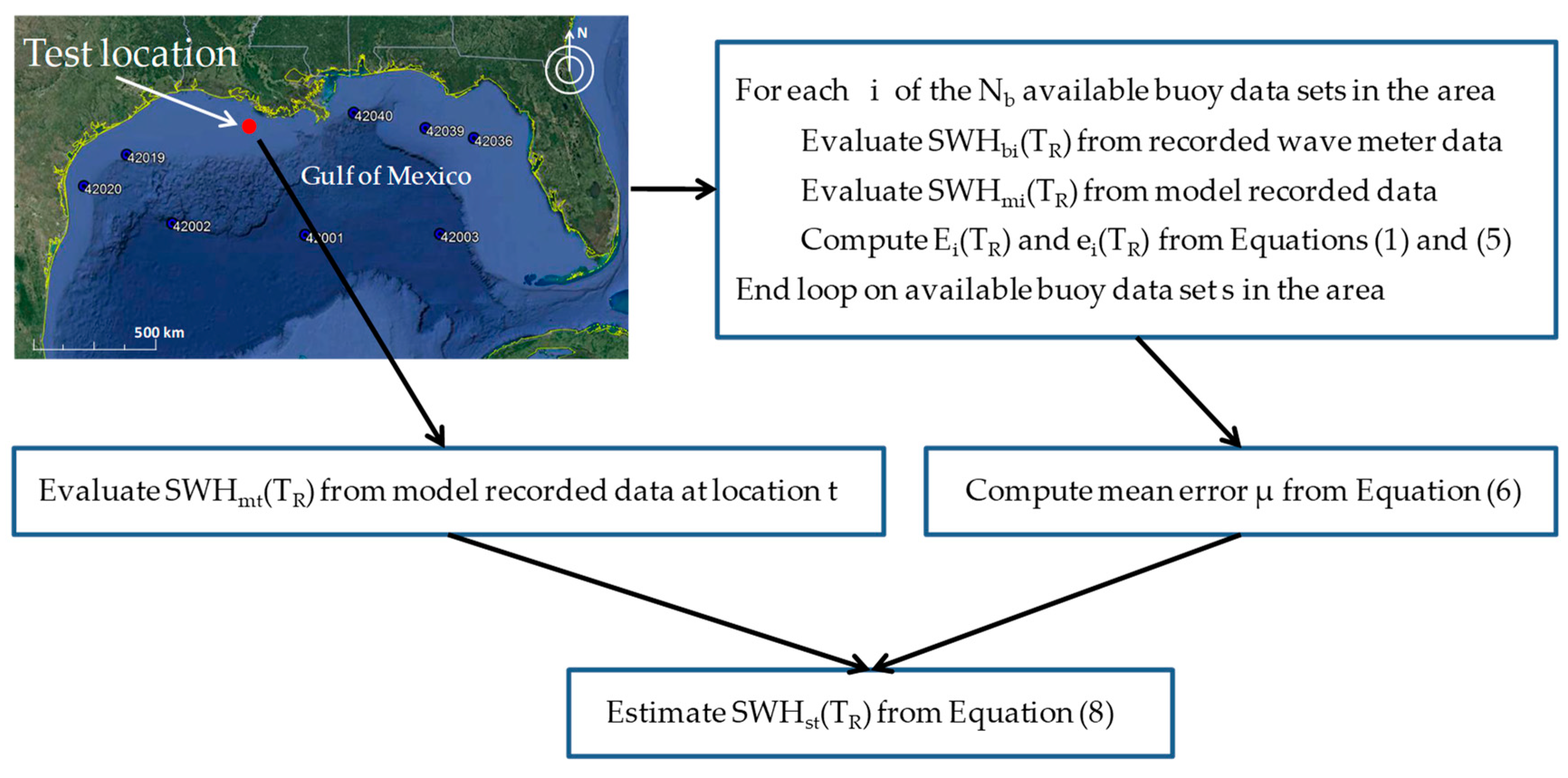
where the sums over the index i being extended to N_b wave buoys considered in the region. Therefore, for a generic location t where no buoy data are available, an estimated SWH_st of the “true” SWH_bt, can be obtained from SWH_mt(T_R) by following Equation (8)

SWH_st(T_R) = SWH_mt(T_R) + µ(T_R) × SWH_mt(T_R),

(8)

where SWH_mt(T_R) is evaluated by using model recorded data at location t.

The integrated procedure, is thus schematically illustrated in Figure 1 for a general test location.

The computational cost of the method is not very high, since it amounts to computing 2N_b + 1 EVPD, an easily standardized and commonly available algorithm, as opposed to a single one, as it would be needed for a conventional procedure based on model data only. The estimation of E_i(T_R), e_i(T_R) and SWH_st(T_R) is straightforward and can be carried out in a single EXCEL^® file.

2.2. Validation

In order to verify the soundness of the procedure and the reliability of the results in a given test location, enough historical data must be available to estimate the experimental true value of the SWH_b(T_R) with a given T_R return time in order to compare it with the estimated value. It is worth recalling that, as stated above, “true” means the value that would be computed from an experimental time series.

In order to do so, the spatial distribution parameters have to be evaluated by making use of a number of wave meters that should not include the test location.

Assuming then that in a given area there are N_b buoys available, the procedure is applied by taking one of them to provide the “true” values at the test location t, while the remaining N_a = N_b − 1 series are used to estimate the relative error distribution e(T_R) according to Equation (5). The procedure highlighted in Figure 1 can thus be applied N_b times, each time choosing in rotation one of the available data series to be taken as test location. Such a methodology, normally called “jackknife” is well known and has been tested in various application [34,35].

For each of the N_b available test locations a corrected estimated return time curve (SWH_st) is thus obtained, and it can be compared with the “true” SWH_bt curve. The following Figure 2 reports an example of the results for NOAA buoy 46014 located along the US Pacific Coast. Here N_b = 8 and therefore N_a = 7.

In Figure 2, the estimated SWH_st is much closer to the buoy value SWH_bt than the model SWH_mt, thus providing a better and safer evaluation of the sea state design value. The same computation can be carried out by rotating the test position among the N_b available buoy locations: this kind of analysis is performed over three test areas described in Section 2.2.

For each test location t the model error (ERM) and the integrated procedure error (ERS), both normalized with the buoy value and indicated as “relative errors”, are computed and defined respectively as:

• ERM = (Model − Buoy)/Buoy = (SWH_mt − SWH_bt)/SWH_bt;
• ERS = (Integrated − Buoy)/Buoy = (SWH_st − SWH_bt)/SWH_bt;
• Improvement = abs(ERM) − abs(ERS).

Improvement, which is the difference between the absolute relative errors, will show how accurate the integrated procedure is compared to the simple application of the model data; all values will be reported in percentage.

2.3. Study Sites

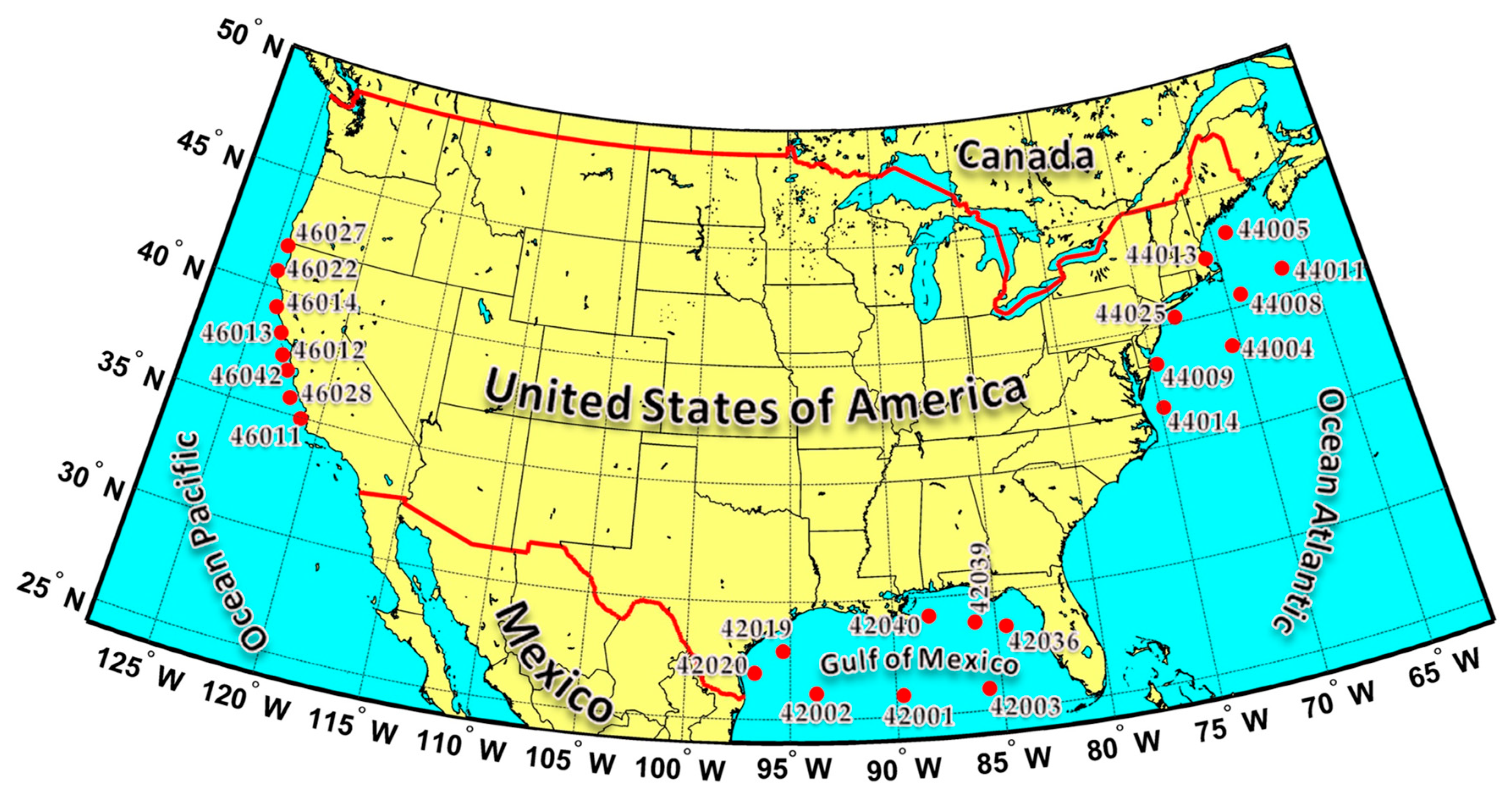
Three areas have been considered for this work: the West (Pacific) Coast and the East (Atlantic) Coast of the United States and the Gulf of Mexico, indicated in the following respectively as PC, AC and GoM. The reason for this choice is the availability of long and good quality wave buoy records given by NOAA (National Oceanic and Atmospheric Administration) National Data Buoy Center (NDBC) [36]. Figure 3 reports the areas considered with the geographical location of the buoys, and their relative NOAA-NDBC identification code number. All the data records are approximately 30 years long and the sampling rate is one hour.

Model data are obtained from the climate forecast system (CFS), run by NOAA National Center for Environmental Prediction (NCEP) [37], which produced the CFS Reanalysis (CFSR) dataset, i.e., a reanalysis of the sea and atmosphere state for the period of 1979 to 2009, on all grid points and with a 3-hourly time resolution. For this study we used the two following 10’ × 10’ nested grid data sets:

• Gulf of Mexico and NW Atlantic 10 min (ecg_10m) for buoys located in Gulf of Mexico and along US Atlantic Coast;
• US West Coast 10 min (wc_10m) for buoys located along US Pacific Coast.

The integrated procedure had already been applied for some of the GoM area buoys in [4], but here for the first time a jackknife validation as described in Section 2.2 is carried out. The model data have also been updated to the most recent version (Phase 2) of CFSR dataset, which was not yet available at the time.

3. Results

The most important result of the work is the comparison between SWH(T_R) evaluated through the different procedures for each zone:

• SWH_bt through wave meter data;
• SWH_mt through model data;
• SWH_st through integrated procedure proposed here.

The metrics “ERM”, “ERS” and “Improvement” as defined in Section 2.2 are also reported.

3.1. Pacific Coast

Results are reported in

Table 1. Pacific Coast: results for T_R = 50 years.

Test Location	SWHbt (m)	SWHmt (m)	SWHst (m)	ERM (%)	ERS (%)	Improvement (%)
46011	9.34	7.47	9.72	−20.03	4.06	15.97
46012	9.53	8.05	10.55	−15.53	10.72	4.81
46013	9.90	8.02	10.45	−19.01	5.57	13.44
46014	10.86	8.56	11.12	−21.25	2.41	18.73
46022	11.80	8.81	11.35	−25.36	−3.83	21.53
46027	10.87	7.87	10.09	−27.60	−7.14	20.46
46028	10.11	7.52	9.68	−25.61	−4.20	21.41
46042	10.34	7.62	9.80	−26.29	−5.21	21.09
Mean	10.34	7.99	10.35	−22.57	0.30	17.18

and

Table 2. Pacific Coast: results for T_R = 100 years.

Test Location	SWHbt (m)	SWHmt (m)	SWHst (m)	ERM (%)	ERS (%)	Improvement (%)
46011	9.73	7.78	10.16	−20.04	4.42	15.62
46012	9.91	8.38	11.03	−15.41	11.28	4.13
46013	10.30	8.35	10.92	−18.96	6.02	12.94
46014	11.30	8.89	11.58	−21.30	2.54	18.76
46022	12.32	9.14	11.81	−25.77	−4.10	21.67
46027	11.34	8.15	10.48	−28.15	−7.62	20.52
46028	10.53	7.79	10.06	−25.99	−4.43	21.57
46042	10.81	7.93	10.22	−26.67	−5.43	21.24
Mean	10.78	8.30	10.78	−22.79	0.34	17.06

, while Figure 4 provides some comparisons in graphical forms.

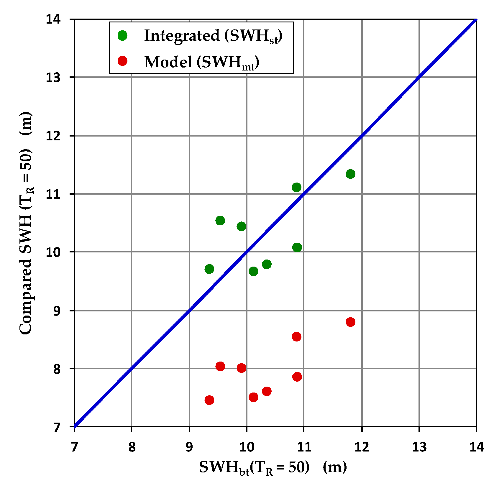
The percentage errors for T_R = 100 are very similar to those computed for T_R = 50. This derives from the similarity of the SWH(T_R) curves for high values of T_R, as noted in Section 2.2 and as shown in Figure 2. The analysis of the results can therefore be limited to just one value of the return periods, i.e., T_R = 50 years. Figure 4 compares the results of the integrated procedure versus the model for T_R = 50 years and provides an insight into the behaviour of the errors.

Figure 4 shows that the values computed with the integrated procedure (green circles) are visibly closer to the values computed with buoy data (blue line) than those computed with the model data (red circles). The low value of the R² between SWH_st and the identity line reflects the dispersion of the error; obviously its average and its extreme values represent a net improvement over the simple model data.

3.2. Atlantic Coast

Numerical results are reported in the following

Table 3. Atlantic Coast: results for T_R = 50 years.

Test Location	SWHbt (m)	SWHmt (m)	SWHst (m)	ERM (%)	ERS (%)	Improvement (%)
44004	13.02	10.07	13.34	−22.64	2.45	20.19
44005	9.91	7.55	9.98	−23.80	0.70	23.09
44008	12.34	9.56	12.66	−22.57	2.56	20.02
44009	9.45	6.65	8.69	−29.60	−8.05	21.55
44011	13.90	10.43	13.75	−24.98	−1.07	23.90
44013	10.04	7.05	9.21	−29.77	−8.31	21.46
44014	10.06	8.21	10.95	−18.41	8.84	9.57
44025	9.02	7.14	9.48	−20.87	5.12	15.76
Mean	10.97	8.33	11.01	−24.08	0.28	19.44

and

Table 4. Atlantic Coast: results for T_R = 100 years.

Test Location	SWHbt (m)	SWHmt (m)	SWHst (m)	ERM (%)	ERS (%)	Improvement (%)
44004	13.75	10.62	14.14	−22.77	2.80	19.97
44005	10.31	7.85	10.43	−23.85	1.16	22.69
44008	13.12	10.12	13.46	−22.90	2.59	20.31
44009	10.13	7.06	9.26	−30.26	−8.57	21.69
44011	15.04	11.23	14.87	−25.35	−1.12	24.23
44013	10.81	7.56	9.91	−30.09	−8.30	21.78
44014	10.72	8.71	11.67	−18.82	8.78	10.04
44025	9.61	7.56	10.09	−21.32	4.99	16.33
Mean	11.69	8.84	11.73	−24.42	0.29	19.68

with the same format and symbols as in Table 1 and Table 2.

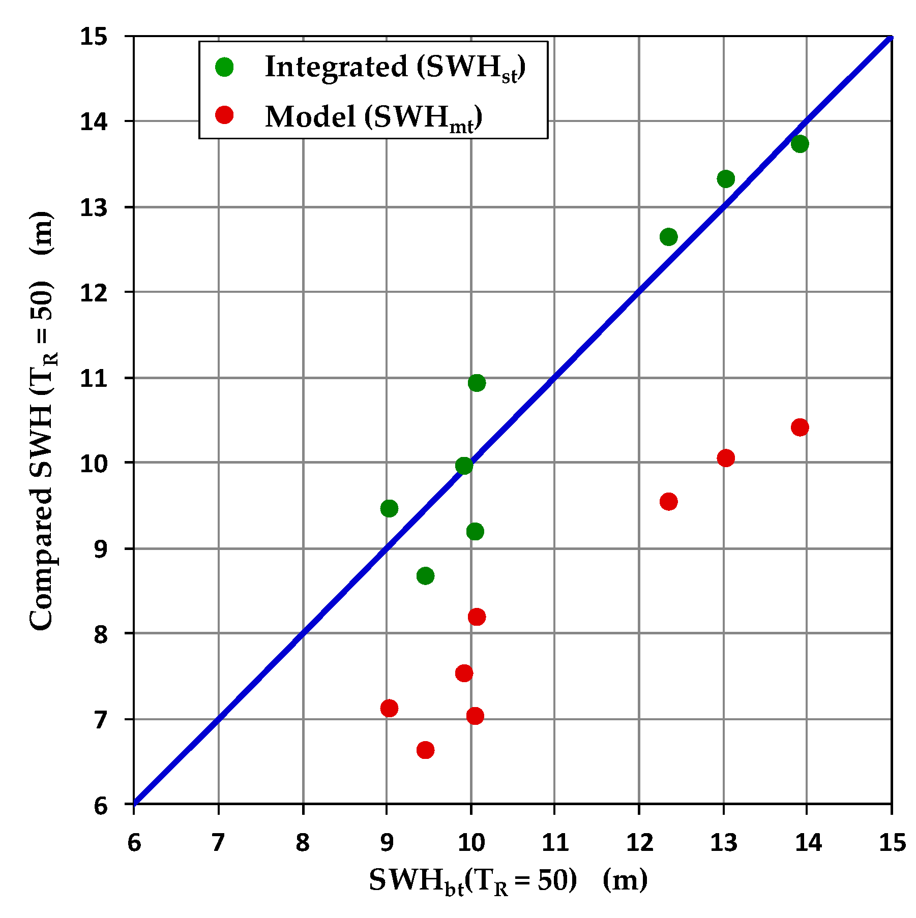
The results of the integrated procedure are compared with the model values and the respective errors are plotted against the true buoy values SWH_bt in Figure 5. The similarity between the results for T_R = 100 and 50 years is also confirmed.

As in the previous case (Figure 4), the improvement is evident with the green circles being much closer to the blue line than the red circles.

3.3. Gulf of Mexico

The following

Table 5. Gulf of Mexico: results for T_R = 50 years.

Test Location	SWHbt (m)	SWHmt (m)	SWHst (m)	ERM (%)	ERS (%)	Improvement (%)
42001	12.31	9.54	11.78	−22.54	−4.33	18.21
42002	9.44	8.47	10.67	−10.30	13.04	−2.74
42003	12.64	10.00	12.38	−20.94	−2.06	18.88
42019	6.77	5.79	7.25	−14.43	7.18	7.25
42020	9.25	7.18	8.86	−22.40	−4.13	18.27
42036	8.80	7.45	9.31	−15.41	5.78	9.63
42039	14.10	11.14	13.80	−20.99	−2.13	18.86
42040	19.21	14.12	17.29	−26.50	−9.96	16.54
Mean	11.57	9.21	11.42	−19.19	0.42	13.11

and

Table 6. Gulf of Mexico: results for T_R = 100 years.

Test Location	SWHbt (m)	SWHmt (m)	SWHst (m)	ERM (%)	ERS (%)	Improvement (%)
42001	13.78	10.60	13.06	−23.09	−5.24	17.85
42002	10.32	9.32	11.74	−9.70	13.74	−4.04
42003	14.14	11.13	13.77	−21.24	−2.62	18.62
42019	7.13	6.16	7.72	−13.52	8.33	5.19
42020	10.16	7.94	9.81	−21.86	−3.49	18.36
42036	9.42	8.00	9.99	−15.14	6.03	9.12
42039	15.83	12.47	15.41	−21.25	−2.63	18.62
42040	21.93	16.09	19.68	−26.63	−10.27	16.54
Mean	12.84	10.21	12.65	−19.05	0.48	12.53

report again the numerical result as in Table 1, Table 2, Table 3 and Table 4.

Figure 6 provides again a plot of the comparison as in Figure 4 and Figure 5.

Note that there is here a single instance (buoy 42002) where for both the T_R considered the absolute values of ERS are greater than correspondent ERM values with consequent negative improvements (−2.74% and −4.04%); however, even in this case, as in all the others, the model results lead to underestimating the SWH_bt(T_R) while the integrated procedure overestimates it, certainly a safer error than the former one. The effectiveness of the integrated procedure in removing the bias of the model is thus confirmed again.

4. Discussion

In considering the results, it should be borne in mind that the object of the investigation is inherently stochastic, since the formation of waves is a natural process driven by meteorological phenomena. The unknown functions SWH(T_R) are the outcome of a statistical elaboration on extreme wave data, and as such they are unavoidably affected by random variations.

The following

Table 7. Mean values of SWH (buoy, model, and integrated) and of metric (ERM, ERS, and Improvement) defined in Section 2.2 for the three areas and two (50 and 100 years) return periods.

Zone	TR (year)	SWHbt (m)	SWHmt (m)	SWHst (m)	ERM (%)	ERS (%)	Improvement (%)
Pacific Cosat	50	10.97	8.33	11.01	−24.08	0.30	17.18
	100	11.69	8.84	11.73	−24.42	0.34	17.06
Atlantic Coast	50	10.34	7.99	10.35	−22.57	0.28	19.44
	100	10.78	8.30	10.78	−22.79	0.29	19.63
Gulf of Mexico	50	11.57	9.21	11.42	−19.19	0.42	13.11
	100	12.84	10.21	12.65	−19.05	0.48	12.53

, which summarises the main results of Section 3, shows that the SWH_mt values, computed through the simple use of model data are systematically affected by an error that is never lower in absolute value than 9.70%, and on average of the order of 20%. Besides, the errors are always negative, i.e., the SWH_mt present a negative bias over the buoy values, so that using model results as design parameters would seriously put any coastal or offshore construction at risk.

It also appears that, as remarked in Section 3.1, the model errors are consistent between the 50 and 100 years return times, since the SWH(T_R) curves portray a similar behaviour for the high values of T_R, which are of interest in practical applications.

A further consideration is that, while the average extreme SWH in the three areas are not too far apart from each other, the model errors are relatively lower in the GoM—most likely reflecting a slightly better performance of the NOAA modelling system in the meteorological conditions of that area.

By applying the integrated procedure, the error ERS decreases to about 0.3–0.5%—a drastic and consistent improvement—even though there are some variations between the various test sites. Only one location (buoy 42002 in GoM, see Table 5 and Table 6) shows a negative improvement, i.e., an error of the integrated procedure which is, in absolute value, slightly (4%) greater than the model error. Additionally, in this case however, the resulting error has a positive value, i.e., the SWH computed with the integrated procedure is higher than the buoy-based value—certainly a safer result.

An inherent negative bias in the model has thus been completely removed. It is worth mentioning that the presence of such a negative bias confirms what had been highlighted in previous work [1,3,25,38], i.e., that the weather/wave models underestimate the extremes despite the constant assimilation of satellite measurement, which due to their coarse temporal and spatial resolution are likely to miss the strongest peaks of the storms.

Considering the inherently stochastic nature of the problem, the results are more than satisfying.

Applying the integrated methodology to any given location requires of course the handling of a considerable amount of data. Simply using model data only requires downloading a single series from one of the available weather/wave systems, such as NOAA [37] or ECMWF [39]; integrating it, if N_b wave buoy are available, requires downloading N_b extra model data series as well as N_b buoy data series. On the other hand, the computational effort is not particularly heavy since the extreme value fitting procedures, briefly recalled in Section 2.1, are nowadays fully standardized.

5. Conclusions

A new procedure, based on integrating wave model data with those obtained with experimental wave data series, has been proposed and tested to evaluate SWH values for a given return time T_R in a given location.

Extreme SWH values derived from model time series are integrated with the corresponding extreme value series from available buoys in the same geographical area.

While of course the calibration or the assimilation of measured wave data with weather/wave model results is nothing new, this is the first time that an integration is carried out to determine the parameters of the SWH extreme value distributions. Such parameters are themselves randomly distributed and they have been estimated by making use of the differences between the SWH obtained from the model and those computed from the in-situ data. In other words, the model data are used as indicators, and the buoy data are used for the correction of biases and the evaluation of uncertainties.

By making use of a jackknife procedure, 24 tests have been carried out on three areas along the coasts of the United States, where long records of good quality buoy data are available. It has been shown that the use of model data always causes a relevant undervaluation of the SWH values for a given return time T_R and that a considerable improvement in accuracy is gained by making use of this integrated procedure in place of using model data.

In a location where there are no buoy wave meters, or where the data series are not long enough for a correct estimate, the integration of the buoy data in the area with model archive data provides a useful and general design tool to derive the extreme value SWH.

Compared with the simple application of a model on the location of interest, the integrated procedure requires a much heavier amount of data, since it implies accessing many time series rather than a single one; on the other hand, the computational burden is not excessive, since it only requires well known and widely accepted procedures for EVPD.

Extension of the method to any other area in the world is certainly possible, provided that a number of wave meter data series in the general area are accessible: while model data are available all over the world, how to identify and evaluate the relevant wave meter buoys is a matter of specific investigation, which should be carried out along the lines outlined here.

References

- Arena, F.; Laface, V.; Barbaro, G.; Romolo, A. Effects of sampling between data of significant wave height for intensity and duration of severe sea storms. Intern. J. Geosci. 2013, 4, 240–248. [Google Scholar] [CrossRef] [Green Version]
- Reale, F.; Dentale, F.; Pugliese Carratelli, E.; Torrisi, L. Remote sensing of small-scale storm variations in coastal seas. J. Coast. Res. 2014, 30, 130–141. [Google Scholar] [CrossRef]
- Dentale, F.; Reale, F.; D’Alessandro, F.; Damiani, L.; Di Leo, A.; Pugliese Carratelli, E.; Tomasicchio, G.R. Sampling Bias in the Estimation of Significant Wave Height Extreme Values. In Proceedings of the 35th Conference on Coastal Engineering, Antalya, Turkey, 17–20 November 2016. [Google Scholar]
- Dentale, F.; Furcolo, P.; Pugliese Carratelli, E.; Reale, F.; Contestabile, P.; Tomasicchio, G.R. Extreme wave analysis by integrating model and wave buoy data. Water 2018, 10, 373. [Google Scholar] [CrossRef] [Green Version]
- Liberatore, G.; Rosso, R. Sulla valutazione stocastica dell’onda di progetto in base alla ricostruzione dello stato del mare: Un esempio di applicazione per l’Adriatico centro-meridionale. G. Genio Civ. 1983, 121, 3–25. (In Italian) [Google Scholar]
- Goda, Y. Statistical Analysis of Extreme Waves. In Random Seas and Design of Maritime Structures, 2nd ed.; Liu, P.L.-F., Ed.; World Scientific Publishing Co. Pte. Ltd.: Singapore, 2000; Volume 15, pp. 377–425. ISBN 981-02-3256-X. [Google Scholar]
- Neelamani, S.; Al-Salem, K.; Rakha, K. Extreme waves for Kuwaiti territorial waters. Ocean Eng. 2007, 34, 1496–1504. [Google Scholar] [CrossRef]
- Muraleedharan, G.; Lucas, C.; Guedes Soares, C.; Unnikrishnan Nair, N.; Kurup, P.G. Modelling significant wave height distributions with quantile functions for estimation of extreme waves heights. Ocean Eng. 2012, 54, 119–131. [Google Scholar] [CrossRef]
- Niroomandi, A.; Ma, G.; Ye, X.; Lou, S.; Xue, P. Extreme value analysis of wave climate in Chesapeake Bay. Ocean Eng. 2018, 159, 22–36. [Google Scholar] [CrossRef]
- Oh, S.-H.; Jeong, W.-M. Extensive monitoring and intensive analysis of extreme winter-season wave events on the Korean east coast. J. Coast. Res. 2014, 70, 296–301. [Google Scholar] [CrossRef]
- Guiberteau, K.; Liu, Y.; Lee, J.; Kozman, T.A. Investigation of developing wave energy technology in the gulf of Mexico. Distrib. Gener. Altern. Energy J. 2012, 27, 36–52. [Google Scholar] [CrossRef]
- Guiberteau, K.; Lee, J.; Liu, Y.; Dou, Y.; Kozman, T.A. Wave energy converters and design considerations for gulf of Mexico. Distrib. Gener. Altern. Energy J. 2015, 30, 55–76. [Google Scholar] [CrossRef]
- Far, S.S.; Wahab, A.K.A.; Harun, S.B. Determination of significant wave height offshore of federal territory of labuan (malaysia) using generalized pareto distribution method. J. Coast. Res. 2018, 34, 892–899. [Google Scholar] [CrossRef]
- Lin-Ye, J.; García-León, M.; Gràcia, V.; Ortego, M.I.; Stanica, A.; Sánchez-Arcilla, A. Multivariate hybrid modelling of future wave-storms at the northwestern black sea. Water 2018, 10, 221. [Google Scholar] [CrossRef] [Green Version]
- Viselli, A.M.; Forristall, G.Z.; Pearce, B.R.; Dagher, A.J. Estimation of extreme wave and wind design parameters for offshore wind turbines in the Gulf of Maine using a POT method. Ocean Eng. 2015, 104, 649–658. [Google Scholar] [CrossRef] [Green Version]
- Pastor, J.; Liu, Y.; Dou, Y. Wave Energy Resource Analysis for Use in Wave Energy Conversion. In Proceedings of the 36th Industrial Energy Technology Conference (IETC 2014), New Orleans, LA, USA, 20–23 May 2014. [Google Scholar]
- Pastor, J.; Liu, Y. Wave climate resource analysis based on a revised gamma spectrum for wave energy conversion technology. Sustainability 2016, 8, 1321. [Google Scholar] [CrossRef] [Green Version]
- Vicinanza, D.; Contestabile, P.; Ferrante, V. Wave energy potential in the north-west of Sardinia (Italy). Renew. Energy 2013, 50, 506–521. [Google Scholar] [CrossRef]
- Shao, Z.; Liang, B.; Li, H.; Lee, D. Study of sampling methods for assessment of extreme significant wave heights in the South China Sea. Ocean Eng. 2018, 168, 173–184. [Google Scholar] [CrossRef]
- Wei, C.-C.; Hsieh, C.-J. Using adjacent buoy information to predict wave heights of typhoons offshore of Northeastern Taiwan. Water 2018, 10, 1800. [Google Scholar] [CrossRef] [Green Version]
- Hsu, T.-W.; Shih, D.-S.; Li, C.-Y.; Lan, Y.-J.; Lin, Y.-C. A study on coastal flooding and risk assessment under climate change in the Mid-Western Coast of Taiwan. Water 2017, 9, 390. [Google Scholar] [CrossRef]
- Lerma, A.N.; Bulteau, T.; Lecacheux, S.; Idier, D. Spatial variability of extreme wave height along the Atlantic and channel French coast. Ocean Eng. 2015, 97, 175–185. [Google Scholar] [CrossRef]
- Li, J.; Pan, S.; Chen, Y.; Fan, Y.-M.; Pan, Y. Numerical estimation of extreme waves and surges over the northwest Pacific Ocean. Ocean Eng. 2018, 153, 225–241. [Google Scholar] [CrossRef]
- Liu, G.; Chen, B.; Gao, Z.; Fu, H.; Jiang, S.; Wang, L.; Yi, K. Calculation of joint return period for connected edge data. Water 2019, 11, 300. [Google Scholar] [CrossRef] [Green Version]
- You, Z.-J.; Yin, B.; Ji, Z.; Hu, C. Minimisation of the uncertainty in estimation of extreme coastal wave height. J. Coast. Res. 2016, 75, 1277–1281. [Google Scholar] [CrossRef]
- Sartini, L.; Mentaschi, L.; Besio, G. Comparing different extreme wave analysis models for wave climate assessment along the Italian coast. Coast. Eng. 2015, 100, 37–47. [Google Scholar] [CrossRef]
- Sartini, L.; Besio, G.; Dentale, F.; Reale, F. Wave Hindcast Resolution Reliability for Extreme Analysis. In Proceedings of the 26th International Ocean and Polar Engineering, Rhodes, Greece, 26 June–2 July 2016; International Society of Offshore and Polar Engineers (ISOPE): Cupertino, CA, USA, 2016. [Google Scholar]
- Vanem, E. Uncertainties in extreme value modelling of wave data in a climate change perspective. J. Ocean Eng. Mar. Energy 2015, 1, 339–359. [Google Scholar] [CrossRef] [Green Version]
- Salvadori, G.; Tomasicchio, G.R.; D’Alessandro, F. Practical guidelines for multivariate analysis and design in coastal and off-shore engineering. Coast. Eng. 2014, 88, 1–14. [Google Scholar] [CrossRef]
- Beyá, J.; Álvarez, M.; Gallardo, A.; Hidalgo, H.; Winckler, P. Generation and validation of the Chilean waves Atlas database. Ocean Model. 2017, 116, 16–32. [Google Scholar] [CrossRef]
- Pelosi, A.; Furcolo, P. An amplification model for the regional estimation of extreme rainfall within orographic areas in campania region (Italy). Water 2015, 7, 6877–6891. [Google Scholar] [CrossRef] [Green Version]
- Mathiesen, M.; Goda, Y.; Hawkes, P.J.; Mansard, E.; Martín, M.J.; Peltier, E.; Thompson, E.F.; Van Vledder, G. Recommended practice for extreme wave analysis. J. Hydraul. Res. 1994, 32, 803–814. [Google Scholar] [CrossRef]
- Anderson, E. User Guide to ECMWF Forecast Products. Available online: https://www.ecmwf.int/sites/default/files/User_Guide_V1.2_20151123.pdf (accessed on 28 February 2018).
- Efron, B.; Stein, C. The jackknife estimate of variance. Ann. Statist. 1981, 9, 586–596. [Google Scholar] [CrossRef]
- Kottegoda, N.T.; Rosso, R. Statistics, Probability, and Reliability for Civil and Environmental Engineers, 1st ed.; McGraw-Hill College: New York, NY, USA, 1998. [Google Scholar]
- NOOA National Data Buoy Center. Available online: https://www.ndbc.noaa.gov/ (accessed on 10 March 2020).
- Environmental Modeling Center—WAVEWATCH III 30-Years Hindcasts Phase 2. Available online: https://polar.ncep.noaa.gov/waves/hindcasts/nopp-phase2.php (accessed on 10 March 2020).
- Cavaleri, L. Wave Modeling-Missing the Peaks. J. Phys. Oceanogr. 2009, 39, 2757–2778. [Google Scholar] [CrossRef]
- ECMWF (European Centre for Medium-Range Weather Forecasts) Wave Model. Available online: https://www.ecmwf.int/en/ecmwf-archive-catalogue (accessed on 10 April 2020).
Figure 1.
Integrated workflow to evaluate SWHst at location t for TR return time.
Figure 2.
Example of results for test location on the site of buoy 46014 along US Pacific Coast: SWHbt is the curve computed from experimental data; SWHmt is the curve computed from model data; SWHst is the estimated curve, obtained through the integrated procedure.
Figure 3.
Study areas with relative NOAA-NDBC buoys location and their identification code number.
Figure 4.
Pacific Coast error analysis for TR = 50 years: SWH(TR) values computed through model data (red circles) and integrated procedure (green circles) are compared with SWH(TR) values computed through buoy data (solid blue line). R2 between SWHst and the identity line 0.0076.
Figure 5.
Atlantic Coast error analysis for TR = 50 years: SWH(TR) values computed through model data (red circles) and integrated procedure (green circles) are compared with SWH(TR) values computed through buoy data (solid blue line). R2 between SWHst and the identity line 0.911.
Figure 6.
Gulf of Mexico error analysis for TR = 50 years: SWH(TR) values computed through model data (red circles) and integrated procedure (green circles) are compared with SWH(TR) values computed through buoy data (solid blue line). R2 between SWHst and the identity line 0.925.