Landsat Hourly Evapotranspiration Flux Assessment using Lysimeters for the Texas High Plains

Abstract

Evapotranspiration (ET) is one of the biggest data gaps in water management due to limited ET measurements, and further, spatial variability in ET is difficult to capture. Satellite-based ET estimation has great potential for water resources planning as it allows estimation of agricultural water use at field, landscape, and watershed scales. However, uncertainties with satellite data derived ET are a major concern. This study evaluates hourly satellite-based ET from 2001–2010 for the growing season (May–October) under irrigated and dryland conditions for both tall and short crops. The evaluation was conducted using observed ET from four large weighing lysimeters at the United States Department of Agriculture Agricultural Research Service (USDA-ARS) Conservation and Production Research Laboratory in Bushland, Texas. Hourly ET from satellite data were derived using the Mapping Evapotranspiration at High Resolution with Internalized Calibration (METRIC) model. Performance statistics showed that satellite-based hourly estimates compared to lysimeter measurements provided good performance with an root-mean-square error(RMSE) of 0.14 mm, Nash–Sutcliffe efficiency (NSE) of 0.57, and R² of 0.62 for ET for dryland crops, and RMSE of 0.16, NSE of 0.63, and R² of 0.65 for irrigated crops. METRIC provided accurate hourly ET estimates that may be useful for irrigation scheduling and other water resources management purposes based on the hourly assessment.

1. Introduction

Evapotranspiration (ET) is one of the major components of the water budget. It plays a major role in the water cycle and irrigation water management [1,2]. Further, ET is the main consumer of rainfall and irrigation water in irrigated agricultural fields in arid and semiarid regions of the world. ET measurement methods such as pan evaporation, sap flow, and weighing lysimeters are widely used. These measurements are considered point estimates for particular irrigation practices in a homogenous field. Measuring ET on a watershed scale is challenging due to unavailability of direct measurement methods at that scale [3,4]. Other ET methods such as Bowen ratio, scintillometers, and eddy covariance can provide greater spatial coverage but may not adequately represent a watershed scale. Remote sensing models using satellite data can provide large-scale spatial coverage at various spatial resolutions [5,6]. Considering the limitation that multiple weather parameters are required for ET modeling (air temperature, relative humidity, and wind speed), uncertainties also exist with satellite ET estimates [7].

Weighing lysimeters are considered the most accurate method for measurement for ET [8,9] as they directly measure the change in mass of a representative soil volume as ET occurs. Lysimeters vary in size, design, and weighing method but have shown applicability to a variety of crops, fruit trees, and forests [10]. Large weighing lysimeters can have sufficient depth and surface area as to not impede crop and root growth; however, shallower or smaller lysimeters may cause restrictions on plant development in addition to affecting drainage and soil water dynamics. These issues can cause discrepancies between the field surrounding the lysimeters or between different lysimeters. However, properly designed and maintained lysimeters can be managed in such a way that the conditions on the lysimeter are the same as the surrounding field, giving field-scale, directly measured ET data. These data still may not be representative of various land uses and management methods at a watershed scale; however, they can provide enough spatial resolution for validation of other ET measurements, such as remote sensing models.

Remote-sensing (RS)-based ET models are better suited than point estimates for estimating crop water use at a regional scale [11]. Numerous remote-sensing-based ET algorithms with varying complexities have been developed and are available for estimating the magnitude and trends in regional ET [12]. Daily, weekly, monthly, and seasonal ET estimation are the most dominant temporal resolutions using remote sensing for regional and watershed scales [13,14]. Gowda et al. [12] reported that daily ET estimates differed by 3 to 35% compared to ET measurements obtained using Bowen ratio and EC methods. Error sources include: (a) modeling errors and (b) measurement uncertainties and discrepancies in model-measurement scales, which are often not adequately accounted for in model testing studies. Errors are associated with all ET determination methods, but many can be minimized by increasing measurement accuracy and by careful quality assessment and quality control of ancillary data [12,15].

Accurate testing of field surface energy balance models, including those based on thermal imagery, depends on the ground truth and remotely sensed data accuracy. At watershed and basin scales, few examples of calibration of satellite-based ET using ground truth data measurements have occurred. These studies used ground truth from mass balance methods, including weighing lysimeters and the soil water balance, and EC measurements based on the energy balance to perform analysis on RS-based energy balance estimates of ET.

One of the major sources of ET estimation uncertainty using satellite energy balance models is the hourly satellite calibration [16,17]. This uncertainty can be minimized by comparing the hourly satellite estimates of evapotranspiration (ET), surface temperature (T_s), net solar radiation (R_n), and soil heat flux (G_o) to the measurements. This calibration is achieved for each image to reduce bias with radiometric accuracy related to the changing aerodynamics of the satellite scene, thermal conditions, and bias related to modeler estimates of the extreme conditions (dry and wet pixels). A dry pixel is described as bare agricultural soil, with high temperature and low evaporation rate, and a wet pixel is described as fully covered agricultural soil, with low temperature and high transpiration rate.

Hourly ET assessment has many benefits, including understanding sources of uncertainty with daily, weekly, monthly, seasonal, and yearly ET estimation. Accuracy assessment of hourly ET is a major step to quantify estimation errors with irrigation water management practices.

This study evaluated the hourly ET estimates of a 10-year period since the hourly estimates are the main component for various time scale ET interpolations. Previous studies evaluated daily, monthly, seasonal, and/or yearly ET estimates; however, no existing study has evaluated the hourly ET for irrigation management purposes. Evaluating hourly ET estimates is crucial to quantify uncertainties associated with the daily, monthly, seasonal, and yearly estimates for irrigation management purposes.

2. Materials and Methods

2.1. Site Description

Four fields equipped with lysimeters at the USDA-ARS Conservation and Production Research Laboratory at Bushland, TX (35.19° N, 102.10° W) at an elevation of 1170 m above mean sea level were selected for this study. The research field is a square with a surface area of approximately 20 ha, subdivided into four quadrants of approximately 4.7 ha each. A precision, large weighing lysimeter is located at the center of each quadrant; two lysimeters were managed as dryland (NW and SW), and the other two lysimeters were managed as irrigated (NE and SE) during the study years. The observed data were combined for each lysimeter, and statistical performance assessment was performed for the estimated values for each parameter for the two dryland lysimeters (NW and SW) and the two irrigated lysimeters (NE and SE). The soil characteristics for the study field are deep, well-drained Pullman silty clay loam (fine, mixed, superactive, thermic Torrertic Paleustoll) [18]. The local climate is classified as semi-arid, with large daily temperature variations. Cotton, soybean, grain and silage sorghum, sunflower, and cotton were the predominant crops for the research fields.

2.2. Weather Parameter Measurements

Dataloggers (CR6, Campbell Scientific, Logan, Utah) were used to collect data using the following sensors: air temperature and relative humidity sensor (HMP155, Vaisala, Helsinki, Finland), four soil water sensors (Acclima 315, Acclima Inc., Meridian, Idaho), six soil heat flux plates (HFT-3, Radiation Energy Balance Systems, Bellevue, WA, USA), an infrared thermometer, and a net radiometer (Q*7.1, Radiation Energy Balance Systems, Bellevue, WA, USA) [19]. These sensors were utilized to measure surface temperature, soil heat flux, and net solar radiation over each lysimeter. The QA/QC protocol from Evett et al. [20] was performed on the collected data. Weather parameter data were recorded every 6 s and summed or averaged for 30-min intervals.

The solar radiation sensor calibration was performed to assess the sensor accuracy through evaluating the observed R_n with the sum of measured downwelling and upwelling short- and longwave radiation as well as comparing to the theoretical maximum clear sky solar irradiance. Based on the sensor calibration results, the sensor performance was accurate in solar radiation measurement.

Colaizzi et al. [21] highlighted the soil heat flux calculation and calibration process for 30-min time intervals. The calibration process was performed using the soil water and temperature sensor data to calculate the change in soil heat storage from the surface to the soil heat flux plates.

2.3. Landsat Imagery

Landsat Collection-1 was used for Landsat 5 Thematic Mapper (TM) satellite data throughout the growing season (May–October). The images were obtained through Earth Explorer (https://earthexplorer.usgs.gov/), with two satellite paths (30 and 31) and row 36 from 2001 to 2010. A total of 53 cloud-free images were acquired, as the presence of clouds can cause errors in the estimation process due to aerodynamics and radiometric disturbance [17]. Supplementary Materials includes day of year (DOY) for images used. The Landsat 5 TM consists of six spectral bands (bands 1–5 and band 7) with spatial resolutions of 30 m and one thermal band (band 6) with a spatial resolution of 120 m. Top-of-atmosphere reflectance was used to calculate NDVI Equation (5) using the red and near-infrared bands [22].

2.4. Image Analysis

The Bushland Evapotranspiration and Agricultural Remote Sensing (BEARS) software is an image processing and geographic information system software deriving hourly, daily, and seasonal evapotranspiration maps. It also produces other energy exchange outputs between land and atmosphere using Landsat 5, 7, and 8 [23]. The BEARS software was used for this analysis to estimate the hourly ET, T_s, R_n, and G_o for the four lysimeters. The BEARS software is public domain software that offers users the option to select one of five energy-balance-based ET methods: Mapping Evapotranspiration at High Resolution with Internalized Calibration (METRIC), Surface Energy Balance Algorithm for Land (SEBAL), Surface Energy Balance System (SEBS), Tow Source Model (TSM), and Simplified Surface Energy Balance (SSEB). The METRIC model has been utilized in this study. To extract the average value of each parameter, a grid of 3 by 3 pixels was selected, with each lysimeter located towards the center of this grid.

The Mapping Evapotranspiration at High Resolution with Internalized Calibration (METRIC) model is a satellite image processing model that is used for ET estimation as a residual of the energy balance for various short crops, tall crops, trees, and forest [24,25,26,27,28,29,30,31,32] Equation (1).

$$E=R_n-G-H$$

(1)

where $LE$ is the latent heat flux density [W m⁻²], $R_n$ is the net radiation [W m⁻²], $G$ is the soil heat flux [W m⁻²], and $H$ is the sensible heat flux density [W m⁻²].

METRIC has been employed for Landsat image analysis (with a spatial resolution of 30 m) for agricultural water use and other agricultural applications that require field-scale resolution. The energy balance is evaluated internally under two extreme conditions (dry and wet) using surface temperature, vegetation growth, and available weather data. The accuracy of ET estimation depends on user experience, and the estimation accuracy was found to be inversely related with ET levels, where low ET levels had high uncertainty and vice versa [33]. Those two extremes are the strength of METRIC, compared to the Surface Energy Balance System (SEBS) and other satellite-based ET models [25]. An automated statistical calibration method has been developed to better estimate the dry and wet pixels, enhancing ET estimation accuracy [17].

Atmospheric correction is not required for surface temperature ($Ts$) and reflectance (albedo) measurements using radiative transfer models due to the use of the indexed temperature gradient $dT$ and the internal calibration of the sensible heat computation within METRIC [34]. Another advantage of using the internal calibration is that it reduces the bias with aerodynamic stability corrections and surface roughness.

Net radiation at the surface ($R_n)$ is calculated by subtracting all outgoing radiant fluxes from all incoming radiant fluxes including solar and thermal radiation Equation (2):

$$R_n=R_{S\downarrow }-\alpha R_{S\downarrow }+R_{L\downarrow }-R_{L\uparrow }-\left(1-{\epsilon }_o\right)R_{L\downarrow }$$

(2)

where $R_{S\downarrow }$ is the incoming short-wave radiation [${\mathrm{W} \mathrm{m}}^{-2 }$], $\alpha$ is the surface albedo (dimensionless), $R_{L\downarrow }$ is the incoming long-wave radiation [${\mathrm{W} \mathrm{m}}^{-2 }$], $R_{L\uparrow }$ is the outgoing long-wave radiation [${ \mathrm{W} \mathrm{m}}^{-2 }]$,${\epsilon }_o$ is the broad-band surface thermal emissivity (dimensionless), and $\left(1-{\epsilon }_o\right)R_{L\downarrow }$ is the fraction of incoming long-wave radiation reflected from the surface.

The surface temperature ($T_s$) is calculated for Landsat images using the modified Planck equation, based on Markham [35], with both atmospheric and surface emissivity correction, as shown in Equation (3).

$$T_s=\frac{K_2}{\ln \left[\left({\epsilon }_{NB}\raisebox{1ex}{$K_1$}\!\left/ \!\raisebox{-1ex}{$R_c$}\right.\right)+1\right]}$$

(3)

where $K_1 and K_2$ are constants ($K_1=607.8 and K_2=1261 \left[{\mathrm{W} \mathrm{m}}^{-2 }{\mathrm{sr}}^{-1}{ \mathsf{\mu }\mathrm{m}}^{-1 }\right]$ for Landsat 5), ${\epsilon }_{NB}$ is the narrow-band emissivity corresponding to satellite thermal sensor wavelength band, and $R_c$ is the corrected thermal radiance from the surface using spectral radiance $L_{t,thermal}$ from the thermal band of Landsat.

The corrected thermal radiance ($R_c$) [${\mathrm{W} \mathrm{m}}^{-2 }{\mathrm{sr}}^{-1}{ \mathsf{\mu }\mathrm{m}}^{-1 }$] is calculated using Equation (4) [36]:

$$R_c=\frac{L_{t,thermal}-R_P}{T_{NB}}-\left(1-{\epsilon }_{NB}\right)R_{sky}$$

(4)

where $L_{t,thermal}$ is the spectral radiance of Landsat 5 thermal band [${\mathrm{W} \mathrm{m}}^{-2 }{\mathrm{sr}}^{-1}{ \mathsf{\mu }\mathrm{m}}^{-1 }$], $R_P$ is the path radiance in the 10.4–12.5 $\mathsf{\mu }\mathrm{m}$ band [${\mathrm{W} \mathrm{m}}^{-2 }{\mathrm{sr}}^{-1}{ \mathsf{\mu }\mathrm{m}}^{-1 }$], $T_{NB}$ is the narrow-band emissivity of air (10.4–12.5 $\mathsf{\mu }\mathrm{m}$ range), and $R_{sky}$ is the narrow-band downward thermal radiation from a clear sky [${\mathrm{W} \mathrm{m}}^{-2 }{\mathrm{sr}}^{-1}{ \mathsf{\mu }\mathrm{m}}^{-1 }$].

The normalized difference vegetation index (NDVI) is the ratio of the differences in reflectivity for the near-infrared band and the red band divided by the sum Equation (5).

$$NDVI=\frac{\left({\rho }_{t,nir}-{\rho }_{t,red}\right)}{\left({\rho }_{t,nir}+{\rho }_{t,red}\right)}$$

(5)

where ${\rho }_{t,nir}$ is the reflectance of the near-infrared band, and ${\rho }_{t,red}$ is the reflectance of the red band.

The soil heat flux represents the rate of heat storage in the soil and vegetation as a result of conduction. METRIC calculates $G$ as a ratio $\frac{G}{R_n}$ using Equation (6) [37] to represent values near mid-day.

$$\frac{G}{R_n}=\left(T_s-273.15\right)\left(0.0038+0.0074\alpha \right)\left(1-0.98 NDV{I}^4\right)$$

(6)

where $T_s$ is the surface temperature $(K$), and $\alpha$ is the surface albedo.

Alternatively, [38] developed the ratio $\frac{G}{R_n}$ using soil heat flux data collected by USDA-ARS [39] for an irrigated crop near Kimberly, Idaho, as represented in Equations (7) and (8).

$$\frac{G}{R_n}=0.05+0.18 e^{-0.521 LAI} \left(LAI\ge 0.5\right)$$

(7)

$$\frac{G}{R_n}=1.80\raisebox{1ex}{$(T_s-273.15)$}\!\left/ \!\raisebox{-1ex}{$R_n$}\right.+0.084 (LAI<0.5)$$

(8)

where $LAI$ is the leaf area index, and $T_s$ is the surface temperature.

METRIC sensible heat flux calculation is estimated from the aerodynamic function as listed in Equation (9).

$$H={\rho }_{air }{C}_{P \frac{dT}{r_{ah}}}$$

(9)

where ${\rho }_{air}$ is the air density [${\mathrm{kg} \mathrm{m}}^{-3}$], $C_P$ is the specific heat of air at constant pressure [${\mathrm{J} \mathrm{kg}}^{-1}{\mathrm{K}}^{-1}$], $r_{ah}$ is the aerodynamic resistance [${\mathrm{s} \mathrm{m}}^{-1}$] between two near-surface heights, $z_1 and z_2$ (always 0.1 and 2 m) computed in a particular pixel, and $dT$ is the near-surface temperature difference ($K$) between $z_1 and z_2$.

In METRIC, the $r_{ah}$ calculation uses wind speed extrapolation from blending heights (normally 100 to 200 m) above the ground surface. $dT$ is used in Equation (9) due to complications in estimating surface temperature accurately from satellites, which arise from uncertainties in atmospheric attenuation or contamination and radiometric calibration of the sensor [25]. The surface temperature obtained by the satellite, whether it is a radiometric or kinematic temperature, can also be different by several degrees from the aerodynamic temperature, the main driver for the heat transfer process [3,40,41]. $dT$ can be estimated using Equation (10) [42].

$$dT=a+b{T}_{s datum}$$

(10)

Where $a and b$ are the empirical constants for a given Landsat satellite image, and $T_{s datum}$ is the surface temperature adjusted to a common elevation for each image pixel using a digital elevation model and customized lapse rate.

Determining accurate hot (dry) and cold (wet) pixels is one of the most critical and challenging steps in implementing METRIC to spatially estimate ET [17,33]. A manual selection method was performed to determine the dry and wet pixels using the surface temperature and the NDVI outputs based on the criteria listed in

Table 1. Hot and cold pixel description and constraint limits.

Parameter	Condition	Constraint		Outcome
		Ts	NDVI
Lowest ET	Bare agricultural soil	High	$\le 0.2$	Hot pixel location (x,y)
Highest ET	Cultivated agricultural soil	Low	$\ge 0.7$	Cold pixel location (x,y)

. The manual selection process was performed using the surface temperature (T_s) and NDVI histogram distribution. Obtaining the T_s distribution is necessary to determine the range of the high and low temperature threshold for each image.

Several iterations were implemented to obtain the most accurate hot and cold pixels that met the conditions listed in Table 1. The more accurate the dry and wet pixel determination, the better the ET estimates across the satellite scene. Special consideration of the hot and cold pixel selection, such as avoiding the image edges, as well as the hot and cold pixels distribution across the scene instead of centralizing the pixels toward a specific location was used.

2.5. Statistical Analysis

In addition to visual inspection of observed and simulated ET values for pixels covering lysimeters, the satellite-based ET performance was evaluated for the selected day's images that were available. Various statistical parameters were estimated, including Nash–Sutcliffe efficiency (NSE), root-mean-square error (RMSE), and mean bias error (MBE), to evaluate the relationship strength between simulated and measured values [19,43,44]. RMSE and MBE were calculated using Equations (11) and (12), respectively. Linear regression was performed to determine the coefficient of determination (R²), the slope and intercept, and Nash–Sutcliffe efficiency (NSE; Nash and Sutcliffe, 1970) (Equation (13) [45]. The slope of 1.0, intercept of zero, and R² approaching 1.0 indicates a perfect fit. The MBE provides the ability to determine the deviation between the measured and satellite-based estimates, with MBE = 0 indicating no bias in estimation. The NSE values can range from -∞ to +1, with +1 being a perfect agreement between the model and observed data [46].

$$MSE=\sqrt{\frac{{\sum }_{i=1}^n{\left({\widehat{y}}_{t-}{y}_t\right)}^2}{n}}$$

(11)

$$MBE= \frac{{\sum }_{i=1 }^n( y_t-{\widehat{y}}_{t })}{n}$$

(12)

where $y_t$ = the i-th observed value, ${\widehat{y}}_{t }$ = the i-th simulated value, and $n$ = total number of observations.

$$NSE=1-\frac{{\sum }_i{\left(y_m-y_s\right)}_i{}^2}{{\sum }_i{\left(y_{m,j}-{\overline{y}}_m\right)}^2}$$

(13)

where ${\overline{y}}_m$ is the average measured value, ${\overline{y}}_s$ is the average simulated value, $y_m$ is the measured data on day i, $y_s$ is the simulated output on day $i$, and $j$ represents the rank.

3. Results

Lysimeter Comparison

The METRIC model [25] was used to estimate ET, and an hourly evaluation was performed for surface temperature, solar radiation, soil heat flux, and evapotranspiration (T_s, R_n, G_o, ET). The evaluation process was conducted for tall crops, including forage sorghum and forage corn; short crops including cotton, sunflowers, and soybeans; and bare soil for the dryland and irrigated lysimeters.

Table 2. Performance statistics of surface energy balance components using Mapping Evapotranspiration at High Resolution with Internalized Calibration (METRI)C for dryland lysimeters (NW and SW) from 2001–2010.

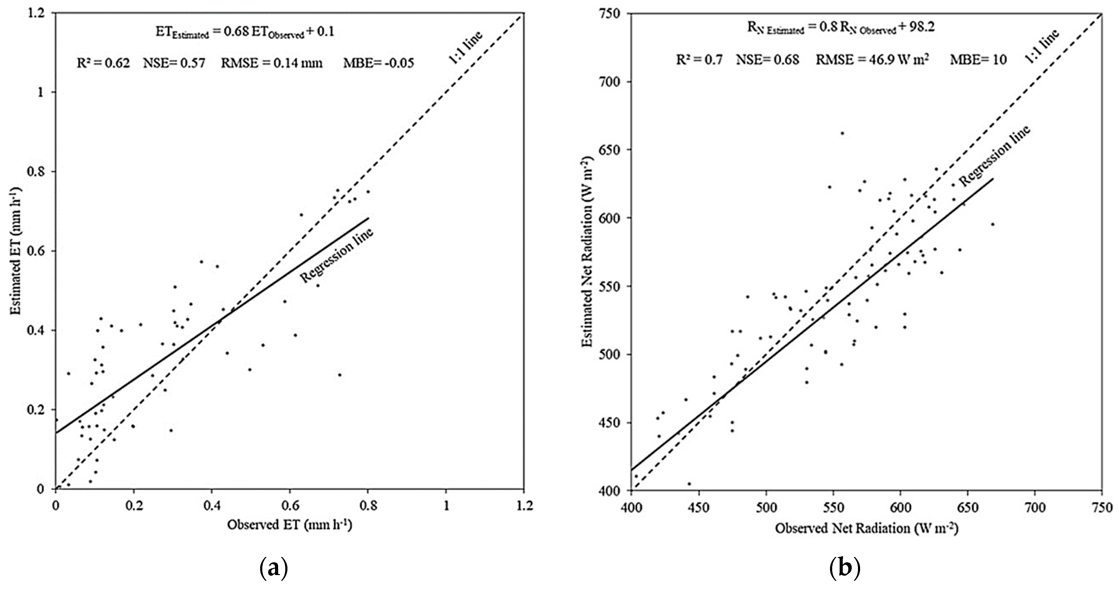
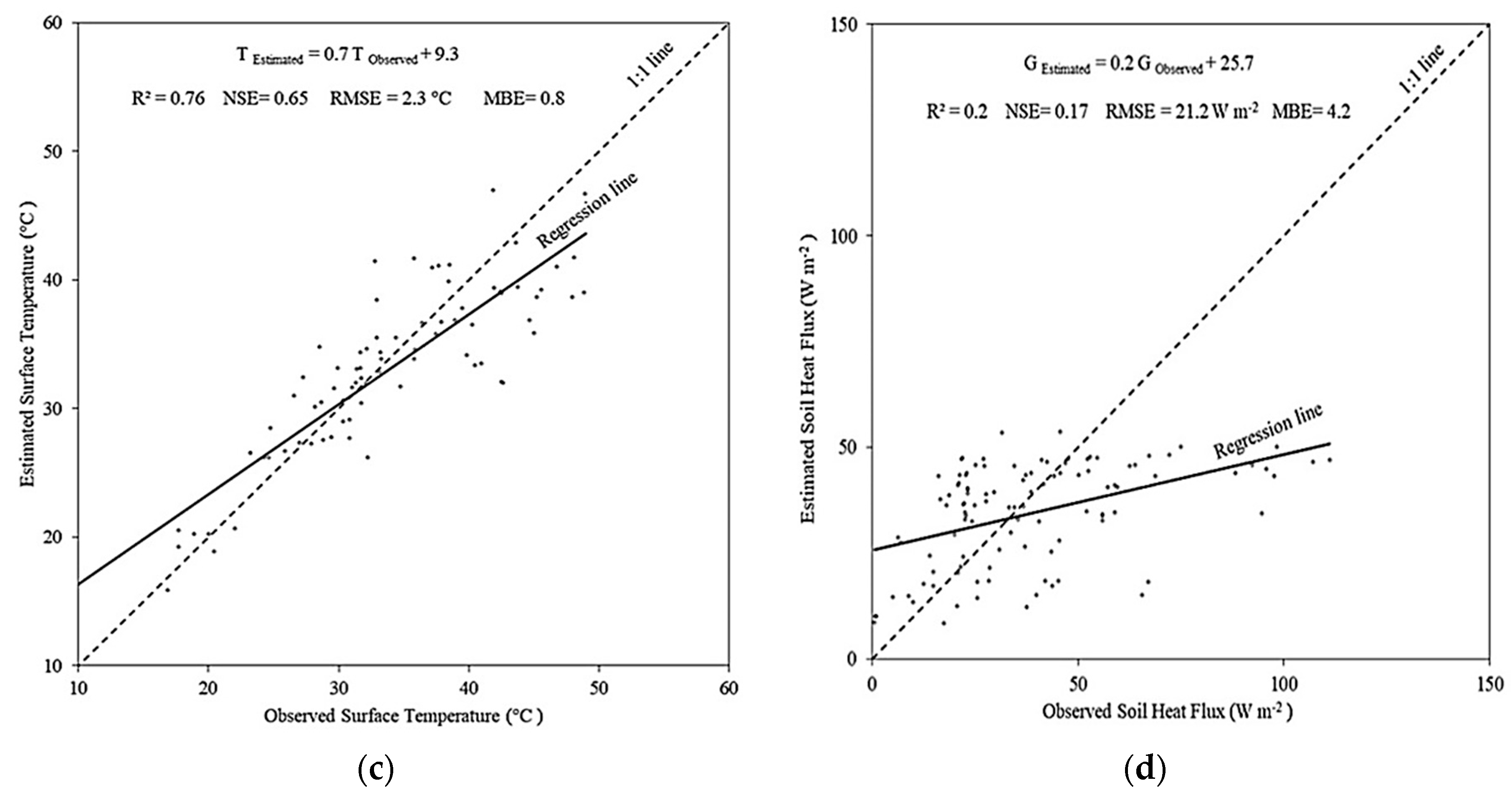
	Mean					Regression
Estimated Parameter	Observed	Estimated	RMSE	MBE	NSE	R2	Slope
T (°C)	33.8	33.0	2.3	0.8	0.65	0.76	0.70
Rn (W m−2)	533.5	521.5	46.9	10.0	0.68	0.71	0.80
Go (W m−2)	38.6	34.5	21.2	4.2	0.17	0.20	0.20
ET (mm h−1)	0.28	0.33	0.14	−0.05	0.57	0.62	0.68

and

Table 3. Performance statistics of surface energy balance components using METRIC for irrigated lysimeters (NE and SE) from 2001–2010.

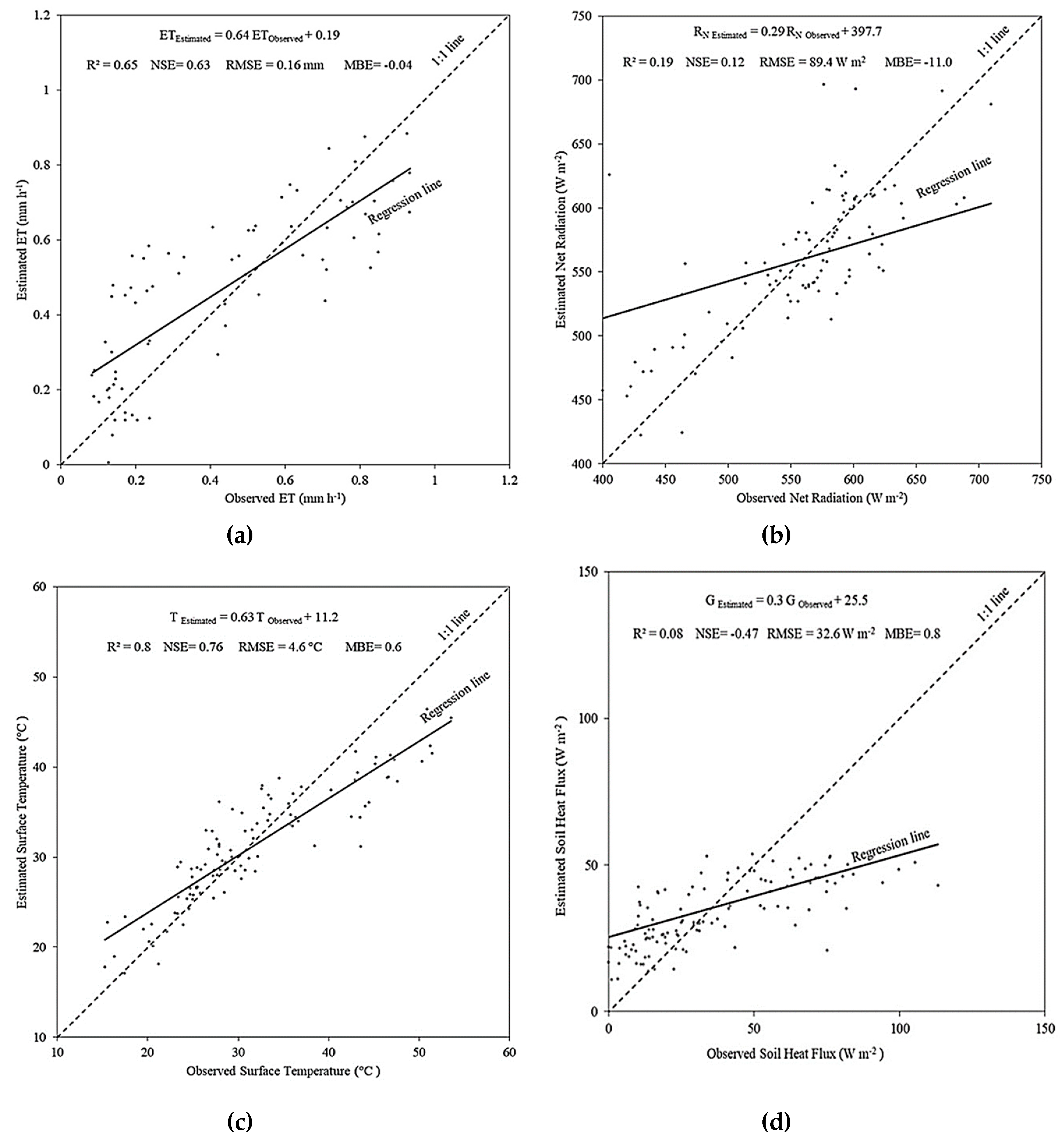
	Mean					Regression
Estimated Parameter	Observed	Estimated	RMSE	MBE	NSE	R2	Slope
T (°C)	31.5	31.2	4.6	0.55	0.76	0.80	0.63
Rn (W m−2)	542.3	551.3	84.8	−9.0	0.17	0.22	0.29
Go (W m−2)	36.4	35.6	32.6	0.8	−0.47	0.08	0.30
ET (mm h−1)	0.43	0.47	0.16	−0.04	0.63	0.65	0.64

summarize the statistical performance of the METRIC model estimation for T_s, R_n, G_o, and ET versus the observed lysimetric data. The regression line between the observed and simulated values for the dryland and irrigated lysimeters can be found in Figure 1 and Figure 2, respectively.

The observed mean hourly surface temperature value for the dryland lysimeter at the time of satellite overpass was 33.8 °C, and it closely matched the estimated mean value of 33.0 °C. The dryland lysimeter regression line for surface temperature had a good coefficient of determination of 0.76, with a slope and intercept of 0.7 and 9.3 °C. The RMSE was ~6.8% (2.3 °C of the mean observed values, with an MBE of 0.8 °C.

Figure 1b and Figure 2b represent the R_n comparison between dryland and irrigated lysimeters, respectively, compared to the measured data. The dryland model estimated R_n value was 521.5${ \mathrm{W} \mathrm{M}}^{-2}$, and it closely matched the measured value of 533.5${ \mathrm{W} \mathrm{M}}^{-2}$. The irrigated lysimeter estimate was 551.3${ \mathrm{W} \mathrm{M}}^{-2}$, and the observed R_n was 542.3 ${\mathrm{W} \mathrm{M}}^{-2}$. The dryland lysimeter model provided good performance for net radiation with an NSE of 0.68 and poor performance for the irrigated lysimeter with an NSE of 0.17. The regression model for dryland lysimeters accounted for 71% of the variability, with a slope of 0.8 and intercept of 98.2 ${\mathrm{W} \mathrm{M}}^{-2}$ (Table 2). The irrigated regression model captured 22% of the variability, which is lower than for the dryland regression model, with a slope of 0.29 and intercept of 392.3 ${\mathrm{W} \mathrm{M}}^{-2}$ (Table 3).

Figure 1d and Figure 2d represent the soil heat flux comparison between dryland and irrigated lysimeters and satellite estimates. Both irrigated and dryland conditions underestimated the soil heat flux compared to the observed values. Consequently, the summary statistics provided a weak correlation for irrigated and dryland lysimeter soil heat flux. The METRIC mean estimated G_o for dryland was 34.5 ${\mathrm{W} \mathrm{M}}^{-2}$ and the observed was 38.6 ${\mathrm{W} \mathrm{M}}^{-2}$, with 10.6% underestimation for the dryland condition. The irrigated lysimeter mean estimated value was 35.6${ \mathrm{W} \mathrm{M}}^{-2}$, and the observed value was 38.6 ${\mathrm{W} \mathrm{M}}^{-2}$, with 2.2% underestimation for the irrigated lysimeter.

The mean hourly estimated ET for dryland was 0.33 mm h⁻¹, and the mean observed ET was 0.28 mm h⁻¹. For the irrigated model, the mean simulated value was 0.47 mm h⁻¹, and the mean observed value was 0.43 mm h⁻¹.

4. Discussion

The hourly comparison for the lysimeter site was performed for surface temperature, evapotranspiration, net radiation, and soil heat flux. The observed surface temperature for the dryland lysimeter was higher than the irrigated lysimeter (Figure 1c and Figure 2c), as expected. The hourly evaluation of the METRIC model illustrated good performance for both water management conditions; however, the irrigated lysimeter overall hourly comparison provided slightly better statistics than the dryland lysimeter. The dryland lysimeter observed and estimated temperatures are higher than for the irrigated lysimeter, and this is due to the irrigation cooling effect.

The observed mean surface temperature value for the irrigated lysimeter was 31.5 °C, and it closely matches the estimated mean value of 31.2 °C. The irrigated lysimeter regression line for surface temperature has better estimates than for the dryland lysimeter, with a coefficient of determination of 0.8, a slope and an intercept of 0.63 and 11.2 °C. The RMSE was 14.6% (4.6 °C) of the mean observed values with MBE of 0.55 °C. These predicted errors are close to those reported in the literature [43,47,48,49,50]. Moorhead and Gowda have similar unpublished reports for METRIC hourly comparisons. The NSE values of 0.65 and 0.76 for the dryland and irrigated surface temperatures, respectively, are viewed as a good match [27,31,43].

The RMSE for the solar radiation for dryland lysimeters was lower than for irrigated lysimeters, with values of 8.8% (46.9${ \mathrm{W} \mathrm{M}}^{-2}$) and 15.6% (84.8${ \mathrm{W} \mathrm{M}}^{-2}$), for the dryland and irrigated lysimeters, respectively. These errors may have resulted from estimation errors in air emissivity and surface albedo as well as the water content in the air above the irrigated field being higher compared to the dryland lysimeter. This water content may distort the electromagnetic reflectance more than for dry fields, resulting in poor solar radiation estimates. These errors ranged within reported values in the literature [31,43,51,52,53,54].

As a result of soil heat flux underestimation, the NSE values were 0.17 and −0.47 for dryland and irrigated lysimeters, respectively, which indicated poor performance for the irrigated field compared to the dryland lysimeter. The RMSE and MBE for the dryland were 55% (21.2 ${\mathrm{W} \mathrm{M}}^{-2}$) and 4.2 ${\mathrm{W} \mathrm{M}}^{-2},$ respectively; the RMSE and MBE for the irrigated lysimeter were 89.6 and 0.8 ${\mathrm{W} \mathrm{M}}^{-2}$, respectively. The dryland regression model accounted for 20% of the variability in measured data with a slope of 0.2 and intercept of 25.7 ${\mathrm{W} \mathrm{M}}^{-2}$ (Table 2). The irrigated regression model accounted for only 8% of variability, with a slope of 0.3 and intercept of 25.5 ${\mathrm{W} \mathrm{M}}^{-2}$ (Table 3). The range of satellite-estimated soil heat fluxes is much lower than that with the observed data, indicating METRIC is underestimating soil heat flux, possibly due to the time difference between the physical process of conduction and the instantaneous acquisition of the satellite image. The wet conditions of the irrigated fields may have an impact on the estimation accuracy of R_n and G₀ due to the humidity above the soil surface. Accuracy in the estimation of R_n and G₀ may be affected by increased humidity near the top of the canopy on the irrigated lysimeter, which may disturb the electromagnetic radiation reflectance compared to the dryland lysimeter. These results agree with [27,31,43].

The METRIC ET estimation provided a good correlation for the dryland model; however, METRIC ET estimation performed better for the irrigated conditions. The hourly ET regression model explained 62% of the ET variability in the observed data for dryland lysimeters, with a slope of 0.68 and an intercept of 0.1 mm h⁻¹. The regression model for irrigated conditions estimated 65% of the variation in the observed data, with a slope of 0.64 and an intercept of 0.19 mm h⁻¹.

The dryland RMSE for the hourly ET was 0.14 mm, which was 50% higher than that of the mean observed ET; the MBE was −0.05 mm. The irrigated modeled hourly ET RMSE was 0.16 mm h⁻¹, about 37.2% higher than that of the mean observed hourly ET; the MBE was −0.04 mm. The irrigated lysimeters error values were less than those of the dryland lysimeter (Table 2 and Table 3), possibly due to increased overall ET and less sensible heat flux, which may have caused attenuation in the reflected radiation from the dryland field as captured by the satellite. Overall, these results agreed with [23,45], illustrating that the accuracy level of METRIC hourly T_s, R_n, and G_o for dryland and T_s and R_n for irrigated lysimeter estimation are considered good for the Texas High Plains, with potential applications for other geographic locations. These results are within the range reported in the literature [12,27,29,30,31,44,54,55,56].

5. Conclusions

The METRIC model was tested against lysimetric hourly surface temperature (T_s), net radiation (R_n), soil heat flux (G_o), and evapotranspiration (ET) in the Texas High Plains. For this purpose, 53 cloud-free images from Landsat 5 TM acquired during 2001–2010 were used. The hourly values were extracted and compared against observed T_s, R_n, G_o, and ET for different (tall and short) crops as well as bare soil conditions managed under dryland and irrigated conditions. The METRIC model performance was good in estimating T_s, R_n, and ET under dryland conditions and T_s and ET for irrigated conditions. The wet conditions in the irrigated lysimeter fields affected electromagnetic reflectance.

The overall accuracy level of the Landsat estimates of the evaluated parameters (surface temperature, net radiation, soil heat flux, and evapotranspiration) indicate that the METRIC model may be suitable for deriving hourly input at a watershed scale with fairly good accuracy.

References

- Sentelhas, P.C.; Gillespie, T.J.; Santos, E.A. Evaluation of FAO Penman-Monteith and alternative methods for estimating reference evapotranspiration with missing data in Southern Ontario, Canada. Agric. Water Manag. 2010, 97, 635–644. [Google Scholar] [CrossRef]
- Gavilán, V.; Lillo-Saavedra, M.; Holzapfel, E.; Rivera, D.; García-Pedrero, A. Seasonal Crop Water Balance Using Harmonized Landsat-8 and Sentinel-2 Time Series Data. Water 2019, 11, 2236. [Google Scholar] [CrossRef] [Green Version]
- Qualls, R.J.; Brutsaert, W. Effect of Vegetation Density on the Parameterization of Scalar Roughness to Estimate Spatially Distributed Sensible Heat Fluxes. Water Resour. Res. 1996, 32, 645–652. [Google Scholar] [CrossRef]
- Ayyad, S.; Al Zayed, I.S.; Ha, V.T.T.; Ribbe, L. The Performance of Satellite-Based Actual Evapotranspiration Products and the Assessment of Irrigation Efficiency in Egypt. Water 2019, 11, 1913. [Google Scholar] [CrossRef] [Green Version]
- PÔças, I.; Paço, T.A.; Cunha, M.; Andrade, J.A.; Silvestre, J.; Sousa, A.; Santos, F.L.; Pereira, L.S.; Allen, R.G. Satellite-based evapotranspiration of a super-intensive olive orchard: Application of METRIC algorithms. Biosyst. Eng. 2014, 128, 69–81. [Google Scholar] [CrossRef] [Green Version]
- Torres-Rua, A.; Ticlavilca, A.; Bachour, R.; McKee, M. Estimation of Surface Soil Moisture in Irrigated Lands by Assimilation of Landsat Vegetation Indices, Surface Energy Balance Products, and Relevance Vector Machines. Water 2016, 8, 167. [Google Scholar] [CrossRef] [Green Version]
- Idso, S.B.; Jackson, R.D.; Reginato, R.J. Estimating evaporation: A technique adaptable to remote sensing. Science 1975, 189, 991–992. [Google Scholar] [CrossRef]
- Evett, S.; Schwartz, R.; Howell, T.A.; Baumhardt, R.L.; Copeland, K.S. Can weighing lysimeter ET represent surrounding field ET well enough to test flux station measurements of daily and sub-daily ET? Adv. Water Resour. 2012, 50, 79–90. [Google Scholar] [CrossRef]
- Howell, T.A.; Schneider, A.D.; Jensen, M.E. History of lysimeter design and use for evaportanspiration measurements. In Proceedings of the International Symposium on Lysimetry, Honolulu, HI, USA, 23–25 July 1991. [Google Scholar]
- Allen, R.; Fisher, D.K. Direct load cell-based weighing lysimeter system. In Proceedings of the International Symposium on Lysimetry, Honolulu, HI, USA, 23–25 July 1991. [Google Scholar]
- Allen, R.G.; Tasumi, M.; Morse, A.; Trezza, R.; Wright, J.L.; Bastiaanssen, W.; Kramber, W.; Lorite, I.; Robison, C.W. Satellite-Based Energy Balance for Mapping Evapotranspiration with Internalized Calibration (METRIC)—Applications. J. Irrig. Drain. Eng. 2007, 133, 395–406. [Google Scholar] [CrossRef]
- Gowda, P.H.; Chavez, J.L.; Colaizzi, P.D.; Evett, S.R.; Howell, T.A.; Tolk, J.A. ET mapping for agricultural water management: Present status and challenges. Irrig. Sci. 2008, 26, 223–237. [Google Scholar] [CrossRef] [Green Version]
- Senay, G.B.; Schauer, M.; Velpuri, N.M.; Singh, R.K.; Kagone, S.; Friedrichs, M.; Litvak, M.E.; Douglas-Mankin, K.R. Long-Term (1986–2015) Crop Water Use Characterization over the Upper Rio Grande Basin of United States and Mexico Using Landsat-Based Evapotranspiration. Remote Sens. 2019, 11, 1587. [Google Scholar] [CrossRef] [Green Version]
- Senay, G.B.; Bohms, S.; Singh, R.K.; Gowda, P.H.; Velpuri, N.M.; Alemu, H.; Verdin, J.P. Operational Evapotranspiration Mapping Using Remote Sensing and Weather Datasets: A New Parameterization for the SSEB Approach. JAWRA J. Am. Water Resour. Assoc. 2013, 49, 577–591. [Google Scholar] [CrossRef] [Green Version]
- Allen, R.G.; Pereira, L.S.; Howell, T.A.; Jensen, M.E. Evapotranspiration information reporting: I. Factors governing measurement accuracy. Agric. Water Manag. 2011, 98, 899–920. [Google Scholar] [CrossRef] [Green Version]
- Allen, R.G.; Pereira, L.S.; Howell, T.A.; Jensen, M.E. Evapotranspiration information reporting: II. Recommended documentation. Agric. Water Manag. 2011, 98, 921–929. [Google Scholar] [CrossRef]
- Allen, R.G.; Burnett, B.; Kramber, W.; Huntington, J.; Kjaersgaard, J.; Kilic, A.; Kelly, C.; Trezza, R. Automated Calibration of the METRIC-Landsat Evapotranspiration Process. J. Am. Water Resour. Assoc. 2013, 49, 563–576. [Google Scholar] [CrossRef]
- Unger, P.W.; Pringle, F.B. Pullman Soils: Distribution Importance, Variability, and Management; Texas Agricultural Experiment Station: College Station, TX, USA, 1981.
- Moorhead, J.E.; Marek, G.W.; Gowda, P.H.; Lin, X.; Colaizzi, P.D.; Evett, S.R.; Kutikoff, S. Evaluation of Evapotranspiration from Eddy Covariance Using Large Weighing Lysimeters. Agronomy 2019, 9, 99. [Google Scholar] [CrossRef] [Green Version]
- Evett, S.R.; Marek, G.W.; Copeland, K.S.; Colaizzi, P.D. Quality Management for Research Weather Data: USDA-ARS, Bushland, TX. Agrosyst. Geosci. Environ. 2018, 1. [Google Scholar] [CrossRef] [Green Version]
- Colaizzi, P.D.; Evett, S.R.; Agam, N.; Schwartz, R.C.; Kustas, W.P.; Cosh, M.H.; McKee, L. Soil heat flux calculation for sunlit and shaded surfaces under row crops: 2. Model test. Agric. For. Meteorol. 2016, 216, 115–128. [Google Scholar] [CrossRef] [Green Version]
- Senay, G.B.; Friedrichs, M.; Singh, R.K.; Velpuri, N.M. Evaluating Landsat 8 evapotranspiration for water use mapping in the Colorado River Basin. Remote Sens. Environ. 2016, 185, 171–185. [Google Scholar] [CrossRef] [Green Version]
- Evett, S.R.; Kustas, W.P.; Gowda, P.H.; Anderson, C.A.; Prueger, J.H.; Howell, T.A. Overview of the Bushland Evapotranspiration and Agricultural Remote sensing EXperiment 2008 (BEAREX08): A field experiment evaluating methods for quantifying ET at multiple scales. Elsevier 2012, 50, 4–19. [Google Scholar] [CrossRef]
- Allen, R.; Morse, A.; Tasumi, M.; Trezza, R.; Bastiaanssen, W.; Wright, J.L.; Kramber, W. Evapotranspiration from a satellite-based surface energy balance for the Snake Plain Aquifer in Idaho. In Proceedings of the USCID Conference, San Luis Obispo, CA, USA, 9–12 July 2002. [Google Scholar]
- Allen, R.G.; Tasumi, M.; Trezza, R.; Morse, A.; Trezza, R.; Wright, J.L.; Bastiaanssen, W.; Kramber, W.; Lorite, I.; Robison, C.W. Satellite-Based Energy Balance for Mapping Evapotranspiration with Internalized Calibration (METRIC)—Model. J. Irrig. Drain. Eng. 2007, 133, 380–394. [Google Scholar] [CrossRef]
- Tasumi, M.; Trezza, R.; Allen, R.G.R.; Wright, J.L.J. Operational aspects of satellite-based energy balance models for irrigated crops in the semi-arid U.S. Irrig. Drain. Syst. 2005, 19, 355–376. [Google Scholar] [CrossRef]
- Hashem, A.A. Irrigation Water Management Using Remote Sensing and Hydrologic Modeling. Ph.D. Thesis, Purdue University, West Lafayette, IN, USA, 2018. [Google Scholar]
- Gowda, P.H.; Terry, A.H.; Jose, L.C.; George, P.; Moorhead, J.E.; Daniel, H.; Marek, T.H.; Porter, D.O.; Marek, G.H.; Colaizzi, P.D.; et al. A Decade of Remote Sensing and Evapotranspiration Research at USDA-ARS Conservation and Production Research Laboratory; American Society of Agricultural and Biological Engineers: St. Joseph, MI, USA, 2015; pp. 1–14. [Google Scholar]
- Santos, C.; Lorite, I.J.; Allen, R.G.; Tasumi, M. Aerodynamic Parameterization of the Satellite-Based Energy Balance (METRIC) Model for ET Estimation in Rainfed Olive Orchards of Andalusia, Spain. Water Resour. Manag. 2012, 26, 3267–3283. [Google Scholar] [CrossRef]
- Numata, I.; Khand, K.; Kjaersgaard, J.; Cochrane, M.; Silva, S. Evaluation of Landsat-Based METRIC Modeling to Provide High-Spatial Resolution Evapotranspiration Estimates for Amazonian Forests. Remote Sens. 2017, 9, 46. [Google Scholar] [CrossRef] [Green Version]
- Madugundu, R.; Al-Gaadi, K.A.; Tola, E.; Hassaballa, A.A.; Patil, V.C. Performance of the METRIC model in estimating evapotranspiration fluxes over an irrigated field in Saudi Arabia using Landsat-8 images. Hydrol. Earth Syst. Sci. 2017, 21, 6135–6151. [Google Scholar]
- El Ghandour, F.-E.; Alfieri, S.M.; Houali, Y.; Habib, A.; Akdim, N.; Labbassi, K.; Menenti, M. Detecting the Response of Irrigation Water Management to Climate by Remote Sensing Monitoring of Evapotranspiration. Water 2019, 11, 2045. [Google Scholar] [CrossRef] [Green Version]
- Morton, C.G.; Huntington, J.L.; Pohll, G.M.; Allen, R.G.; McGwire, K.C.; Bassett, S.D. Assessing Calibration Uncertainty and Automation for Estimating Evapotranspiration from Agricultural Areas Using METRIC. J. Am. Water Resour. Assoc. 2013, 49, 549–562. [Google Scholar] [CrossRef]
- Tasumi, M.; Allen, R.G.; Trezza, R.; Wright, J.L. Satellite-Based Energy Balance to Assess Within-Population Variance of Crop Coefficient Curves. J. Irrig. Drain. Eng. 2005, 131, 94–109. [Google Scholar] [CrossRef]
- Markham, L.B. Landsat MSS and TM post-calibration dynamic ranges, exoatmospheric reflectances and at-satellite temperatures. Landsat Tech. Notes 1986, 1, 3–8. [Google Scholar]
- Wukelic, G.E.G.E.; Gibbons, D.E.; Martucci, L.M.M.; Foote, H.P.P. Radiometric calibration of Landsat Thematic Mapper thermal band. Remote Sens. Environ. 1989, 28, 339–347. [Google Scholar] [CrossRef]
- Bastiaanssen, W.G.M.; Molden, D.J.; Makin, I.W. Remote sensing for irrigated agriculture: Examples from research and possible applications. Agric. Water Manag. 2000, 46, 137–155. [Google Scholar] [CrossRef]
- Tasumi, M. Progress in Operational Estimation of Regional Evapotranspiration Using Satellite Imagery. Ph.D. Thesis, University of Idaho, Moscow, ID, USA, 2003. [Google Scholar]
- Wright, J.L. New evapotranspiration crop coefficients. Proc. Am. Soc. Civ. 1982, 108, 57–74. [Google Scholar]
- Kustas, W.P.; Moran, M.S.; Humes, K.S.; Stannard, D.I.; Pinter, J.; Hipps, L.E.; Swiatek, E.; Goodrich, D.C. Surface energy balance estimates at local and regional scales using optical remote sensing from an aircraft platform and atmospheric data collected over semiarid rangelands. Water Resour. Res. 1994, 30, 1241–1259. [Google Scholar] [CrossRef]
- Norman, J.; Kustas, W.; Humes, K. Source approach for estimating soil and vegetation energy fluxes in observations of directional radiometric surface temperature. Agric. For. Meteorol. 1996, 77, 263–293. [Google Scholar] [CrossRef]
- Bastiaanssen, W.G.M. Regionalization of surface flux densities and moisture indicators in composite terrain: A Remote Sensing Approach under Clear Sskies in Mediterranean Climates. Ph.D. Thesis, Wageningen University, Wageningen, The Netherlands, 1995. [Google Scholar]
- Gowda, P.; Howell, T.; Paul, G.; Colaizzi, P.D.; Marek, T.H.; Su, B.; Copeland, K.S. Deriving hourly evapotranspiration rates with SEBS: A lysimetric evaluation. Vadose Zo. J. 2013, 12, 1–11. [Google Scholar] [CrossRef] [Green Version]
- Hashem, A.A.; Engel, B.A.; Bralts, V.F.; Radwan, S.; Rashad, M. Performance evaluation and development of daily reference evapotranspiration model. Irrig. Drain. Syst. Eng. 2016, 5, 1–6. [Google Scholar]
- Nash, J.E.; Sutcliffe, J.V. River flow forecasting through conceptual models part I - A discussion of principles. J. Hydrol. 1970, 10, 282–290. [Google Scholar] [CrossRef]
- Santhi, C.; Arnold, J.G.; Williams, J.R.; Dugas, W.A.; Srinivasan, R.; Hauck, L.M. Validation Of The SWAT Model On A Large Rwer Basin With Point And Nonpoint Sources. J. Am. Water Resour. Assoc. 2001, 37, 1169–1188. [Google Scholar] [CrossRef]
- Anderson, M.C.; Norman, J.M.; Mecikalski, J.R.; Torn, R.D.; Kustas, W.P.; Basara, J.B.; Anderson, M.C.; Norman, J.M.; Mecikalski, J.R.; Torn, R.D.; et al. A Multiscale Remote Sensing Model for Disaggregating Regional Fluxes to Micrometeorological Scales. J. Hydrometeorol. 2004, 5, 343–363. [Google Scholar] [CrossRef]
- Chávez, J.L.; Gowda, P.H.; Howell, T.A.; Copeland, K.S. Radiometric surface temperature calibration effects on satellite based evapotranspiration estimation. Int. J. Remote Sens. 2009, 30, 2337–2354. [Google Scholar] [CrossRef]
- Elhaddad, A.; Garcia, L.A.; Chávez, J.L. Using a Surface Energy Balance Model to Calculate Spatially Distributed Actual Evapotranspiration. J. Irrig. Drain. Eng. 2011, 137, 17–26. [Google Scholar] [CrossRef]
- Hashem, A.A.; Engel, B.A.; Rashad, M.; Ramadan, M.H.; Radwan, S.M. Development and validation of mathematical model for calculating daily reference evapotranspiration. In Proceedings of the American Society of Agricultural and Biological Engineers, Evapotranspiration: Challenges in Measurement & Modeling from Leaf to the Landscape Scale & Beyond, Raleigh, NC, USA, 7–10 April 2014. [Google Scholar]
- Key, J.R.; Schweiger, A.J.; Stone, R.S. Expected uncertainty in satellite-derived estimates of the surface radiation budget at high latitudes. J. Geophys. Res. C Ocean. 1997, 102, 15837–15847. [Google Scholar] [CrossRef]
- Chávez, J.L.; Howell, T.A.; Copeland, K.S. Evaluating eddy covariance cotton ET measurements in an advective environment with large weighing lysimeters. Irrig. Sci. 2009, 28, 35–50. [Google Scholar] [CrossRef]
- Mkhwanazi, M.; Chávez, J.L.; Rambikur, E.H. Comparison of Large Aperture Scintillometer and Satellite-based Energy Balance Models in Sensible Heat Flux and Crop Evapotranspiration Determination. Int. J. Remote Sens. Appl. 2012, 2, 24. [Google Scholar]
- Mkhwanazi, M.M.; Chávez, J.L. Mapping evapotranspiration with the remote sensing ET algorithms METRIC and SEBAL under advective and non-advective conditions: Accuracy determination with weighing lysimeters. Hydrol. Days 2013, 1, 68–72. [Google Scholar]
- French, A.N.; Hunsaker, D.J.; Thorp, K.R. Remote sensing of evapotranspiration over cotton using the TSEB and METRIC energy balance models. Remote Sens. Environ. 2015, 158, 281–294. [Google Scholar] [CrossRef]
- Long, D.; Singh, V.P. Assessing the impact of end-member selection on the accuracy of satellite-based spatial variability models for actual evapotranspiration estimation. Water Resour. Res. 2013, 49, 2601–2618. [Google Scholar] [CrossRef]