Machine Learning Approaches for Predicting Health Risk of Cyanobacterial Blooms in Northern European Lakes


1
Department of Civil Engineering, University of Thessaly, 38334 Volos, Greece
2
Norwegian Institute for Water Research (NIVA), Gaustadalléen 21, 0349 Oslo, Norway
*
Author to whom correspondence should be addressed.
Water 2020, 12(4), 1191; https://doi.org/10.3390/w12041191
Submission received: 1 April 2020
/
Revised: 16 April 2020
/
Accepted: 17 April 2020
/
Published: 22 April 2020
(This article belongs to the Special Issue Water Resources Management: Advances in Machine Learning Approaches)
Abstract
:Cyanobacterial blooms are considered a major threat to global water security with documented impacts on lake ecosystems and public health. Given that cyanobacteria possess highly adaptive traits that favor them to prevail under different and often complicated stressor regimes, predicting their abundance is challenging. A dataset from 822 Northern European lakes is used to determine which variables better explain the variation of cyanobacteria biomass (CBB) by means of stepwise multiple linear regression. Chlorophyll-a (Chl-a) and total nitrogen (TN) provided the best modelling structure for the entire dataset, while for subsets of shallow and deep lakes, Chl-a, mean depth, TN and TN/TP explained part of the variance in CBB. Path analysis was performed and corroborated these findings. Finally, CBB was translated to a categorical variable according to risk levels for human health associated with the use of lakes for recreational activities. Several machine learning methods, namely Decision Tree, K-Nearest Neighbors, Support-vector Machine and Random Forest, were applied showing a remarkable ability to predict the risk, while Random Forest parameters were tuned and optimized, achieving a 95.81% accuracy, exceeding the performance of all other machine learning methods tested. A confusion matrix analysis is performed for all machine learning methods, identifying the potential of each method to correctly predict CBB risk levels and assessing the extent of false alarms; random forest clearly outperforms the other methods with very promising results.
1. Introduction
Cyanobacterial harmful algal blooms pose a major concern for freshwater and coastal ecosystems worldwide. The occurrence, frequency and duration of cyanobacterial blooms has increased significantly in recent years as eutrophication, a state of high primary productivity, is appearing in more and more lake ecosystems [1,2,3]. Cyanobacteria may potentially produce a variety of toxins (cyanotoxins), responsible for a wide range of adverse environmental and health impacts. As a result, authorities are occasionally forced to block the intended use of lakes in order to protect public health [4,5,6]; indeed, surface freshwater uses, such as water supply, irrigation, fishing and recreation, can be critically affected by the excessive presence of cyanobacteria and raise health safety issues [7]. Moreover, cyanobacteria biomass is a component of the classification system of the ecological status for lakes according to the European Water Framework Directive [8], since a high abundance of cyanobacteria can reduce aquatic biodiversity and food quality for zooplankton. The identification of synergistic factors favoring cyanobacterial abundance in lakes has been the focus of several past and current studies that have highlighted different hydrological, climatic and human-oriented conditions. Cyanobacterial blooms are not a modern phenomenon and have been reported in scientific literature for more than 130 years [9]; however, they tend to appear much more frequently in recent decades, mainly due to anthropogenic activities that tend to change the global climatic and environmental regime. Examples of such activities include changes in hydrological flow pathways, excessive use of fertilizers and the gradual removal of natural buffering zones between terrestrial and freshwater ecosystems [10]. On the contrary, there are some anthropogenic changes, such as flooding and flushing, that tend to reduce the growth of cyanobacteria more than other algae [11].
Empirical modeling has recognized the fundamental effect of phosphorus and nitrogen on the fluctuation of cyanobacterial biomass, incriminating over-enrichment of lakes with nutrients as a major driver of cyanobacterial blooms [12,13,14,15,16]. In addition, high air or water temperature [11,17], calm weather (low wind speed) [18], high water residence time [19,20], low nitrogen-to-phosphorus ratios [21,22] and low light availability [23,24] are documented as significant factors and possible predictors that determine the dominance of cyanobacteria. However, predicting the concentration of cyanobacterial biomass in lakes is a complex and challenging task and this article comes to address this challenge. The evidence to date highlights the ability of cyanobacteria to adapt under different conditions [25], indicating that cyanobacterial response to anthropogenic stressors is likely not identical across lakes. The growth and proliferation of cyanobacteria appears to be triggered under different thresholds of the above-mentioned predictor variables, showing a significant sensitivity to case-specific spatial, hydrological and climatic conditions [26,27,28,29,30]. Otherwise stated, the relative importance of factors influencing the abundance of cyanobacteria, which are characterized by a case-specific and almost idiosyncratic character, varies among different lake ecosystems. This fact makes establishing a generalized prediction methodology difficult. Previous studies have investigated the impact of lake type variables on how cyanobacteria respond to the combined effect of nutrients and water temperature, engaging trophic state [31], mixing type [32], shallow vs. deep lakes and artificial vs. natural lakes [17]. Nevertheless, although different modelling structures influence the outcome of the models used, the predictive power remains questionable and relatively low, failing to explain cyanobacteria dynamics effectively. In this article, we use a novel prediction scheme with four different machine learning methods that allows us to predict cyanobacteria taking into account not only nutrients, but also a series of variables, such as latitude, elevation, surface area and depth, which are indicative of the case-specific nature of lake ecosystems. To our knowledge, this type of analysis is innovative and has not been implemented before. Even though other scientists have used artificial intelligence methodologies to predict cyanobacterial concentrations or algal blooms [33,34], they usually model a single lake ecosystem and have available a long time series of several lake variables. In this article, we use data from 822 Northern European lakes and model their cyanobacteria dynamics as a whole.
According to the World Health Organization (WHO), recreational water safety is defined by a series of guideline values for cyanobacteria, which are associated with incremental severity and likelihood of health impacts [35]. Lake recreational risk assessment is a costly, time-consuming process that requires specially equipped laboratories and skilled personnel for precise testing of the presence and abundance of cyanobacteria. Machine learning algorithms can provide a reliable alternative approach to predicting the risk to human health associated with recreational activities, based on explanatory variables that can be easily measured and obtained at low cost. These classification algorithms are gaining ground due to their ability to effectively “understand” the dataset given and determine which label or category should be given new data by associating patterns to the unlabeled new data. Moreover, linking environmental conditions with cyanobacterial concentrations and assigning them to corresponding risk levels could improve model predictability and inform authorities whether water is appropriate or not to serve specific uses. It is well known that cyanobacterial toxins can cause high acute and chronic toxicities, since they are classified mostly as hepatotoxins and neurotoxins, affecting the liver and nervous system, respectively [36]. The novelty of this article is that it focusses on predicting the relative risk to human health associated with the level of cyanobacterial abundance in fresh waters, facilitating water management.
Validation is an important component of the modelling procedure; however, many of the empirical models presented in the literature lack a consistent validation methodology, which adds controversy on whether they are capable to perform with similar efficiency on different datasets out of the training ones. Training and validating the models used to predict CBB would empower their capability and effectiveness to adequately perform on a different dataset. In this article, we address this gap and perform model validation of the reported results.
In this study, we use a large-scale monitoring dataset compiled from 822 lakes belonging to six Northern European countries to (i) predict cyanobacterial biomass concentration from a series of possible explanatory variables and check the predictive power of multiple regression on the entire dataset and on subsets of shallow and deep lakes by following a 10-fold cross-validation procedure; (ii) investigate through path analysis how nutrients, chlorophyll-a and air temperature affect cyanobacteria by evaluating all possible direct and indirect pathways; and (iii) calibrate, validate and/or optimize a series of machine learning algorithms, namely Decision Tree (DT), K-Nearest Neighbors (k-NN), Support-vector Machine (SVM) and Random Forest (RF), towards the prediction of risk levels to human health associated with the use of lakes for recreational activities.
2. Materials and Methods
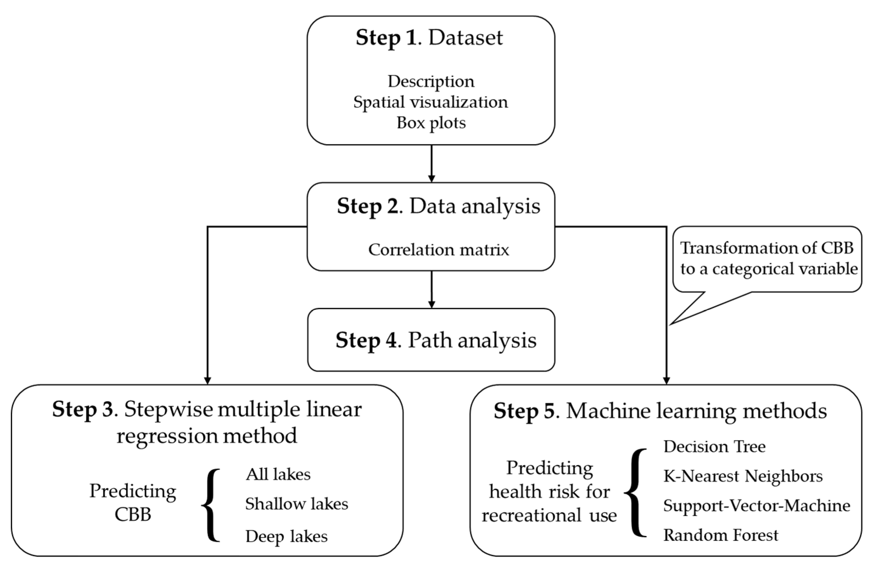
The methodology followed in this study consists of five steps. In Step 1, the dataset is thoroughly described, followed by spatial visualization of variables and box plots for CBB and the main candidate explanatory variables considered in the analysis. In Step 2, a correlation matrix is constructed, and pairwise linear correlation coefficients of all variables are presented. In Step 3, we perform stepwise multiple linear regression in order to define which variables explain most of the variation of CBB; the analysis is done on the whole dataset and on shallow and deep lakes subsets. In Step 4, we continue with path analysis and examine all possible direct and indirect effects of the predictor variables on CBB. Finally, in Step 5, we implement four different machine learning methods to predict the risk to human health associated with the level of cyanobacterial abundance for recreational water use. For this analysis, continuous CBB data are transformed to categorical classifying data in levels that correspond to three distinct health risk levels (low–medium–high), as defined by the WHO for recreational use [35]. In Figure 1, all five steps describing the sequence of the methodology are presented.
2.1. Dataset
The original dataset used in this study, which contains a wide range of hydrological, biological, chemical and geomorphological features of European lakes, was extracted from the central database [37] of the EU-funded project WISER, which aimed at developing integrative systems to assess the ecological status of water bodies according to the Water Framework Directive (WFD) [38]. Under the umbrella of the project, monitoring data from rivers, lakes and coastal waters were compiled from several European research institutions and environmental agencies, to analyze the responses of biological quality elements to physico-chemical stressors under varying environmental conditions. The extracted dataset contained data on the abovementioned features for 1851 lakes, covering the growing season period (from the 5th to 10th month) from 1980 to 2009. However, the dataset exhibited a great heterogeneity in terms of the number and frequency of the observations and monitored features for each lake. Consequently, each lake contributed a variable number of observations and features, for a variable time period and for different months during the growing season. In order to obtain the same number of monitored features per lake, a preliminary screening was conducted that produced an optimized dataset with data for as many features as possible. The resulting dataset consists of 822 lakes from six Northern European countries, namely, the UK, Denmark, Norway, Sweden, Finland and Lithuania. The data include observations for cyanobacteria biomass (CBB, mg/L), chlorophyll-a concentration (Chl-a, μg/L), total nitrogen concentration (TN, μg/L), total phosphorus concentration (TP, μg/L), mean air temperature (MeanATemp, °C), max air temperature (MaxATemp, °C) and the geomorphological characteristics of the lakes—elevation (Elev, m above sea level (a.s.l.)), surface area (SurArea, km2), mean lake depth (MeanDep, m) and maximum lake depth (MaxDep, m). Table 1 summarizes the number of lakes per country included in the dataset, the median and mean number of observations per lake (variable), the sampling months and the corresponding sampling years. As stated above, the dataset is temporally unbalanced, reflecting the different monitoring schemes of the countries that provided data to WISER [39]. For some lakes, there may be a complete dataset covering all sampling months with multiple measurements, while for others we may have a single measurement for the whole time period. To deal with this temporal heterogeneity, there were several options, such as averaging all values to one per lake, selecting only the latest observation per lake, or using a mixed-effects hierarchical model. In this research, no temporal aggregation was applied and all values per lake were used with no weighing/selection. This was done because any type of aggregation would shrink the size of the dataset, a factor that greatly impacts the performance of machine learning algorithms, rendering small datasets unsuitable [40].
Across the Northern European lakes included in the dataset, there is a wide variation in environmental variables. The large geographic extent covers various climatic conditions with the mean air temperature ranging between −0.33 and 21.1 °C. This is a typical temperature variation within the temperate zone and especially within the Atlantic and Continental types of climate. Although the cyanobacteria biomass is low in most lakes, it ranges between 0 and 71.47 mg/L under different combinations of biochemical and geomorphological conditions. The distribution of variables across the lakes in this study is summarized in Table 2, which shows the minimum, maximum, median and mean values for each lake variable.
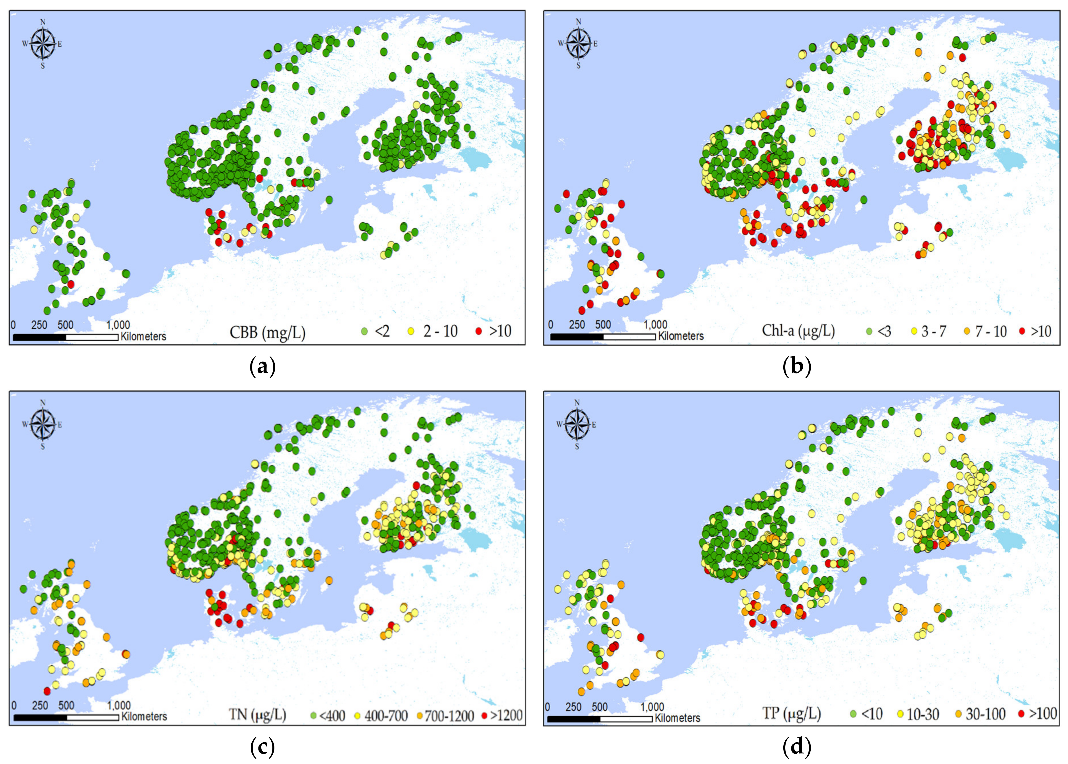
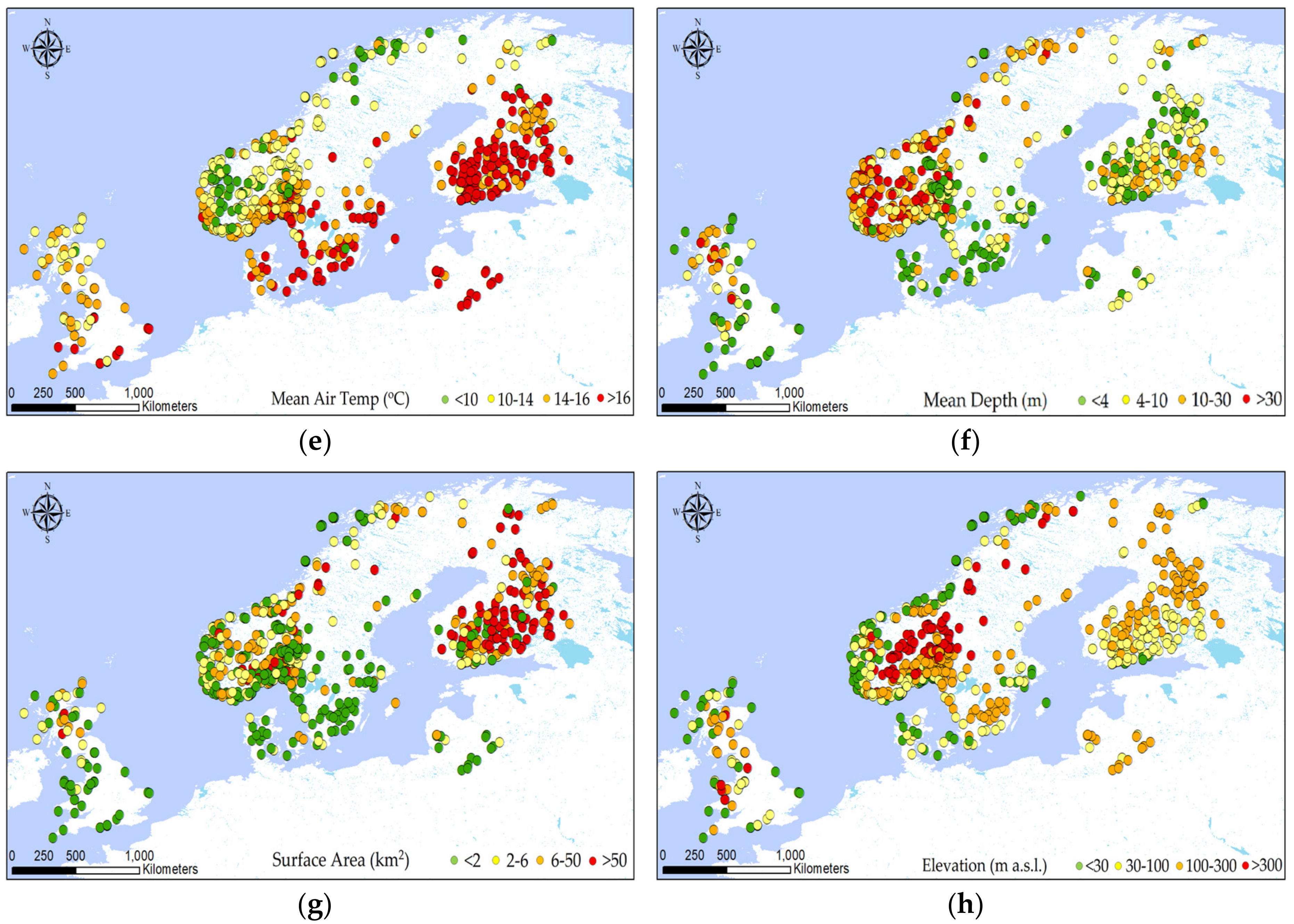
Figure 2 shows the variation in the observed values of the main variables considered for all the lakes under study. Since each lake has one or more observations for each variable, the record with the highest CBB value has been chosen for mapping in the figure. Therefore, for each of the 822 lakes, the visualization was driven by the maximum CBB observed in each lake and the corresponding observations for the remaining variables. The rest of the variables mapped are the ones that correspond to that maximum CBB record for each lake. The analysis was conducted with ArcGIS software.
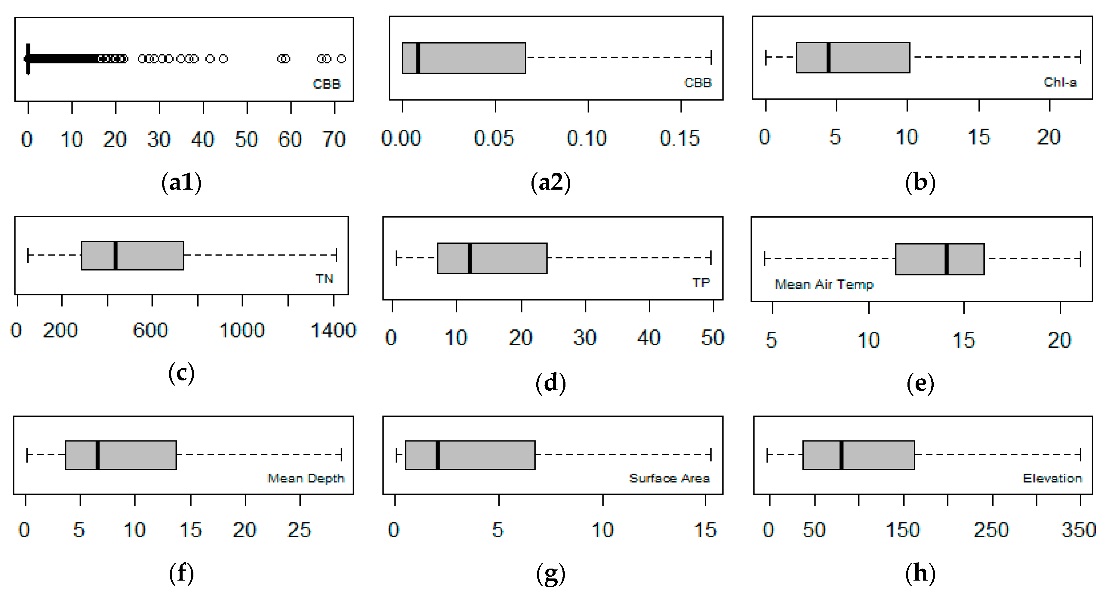
Exploratory data analysis was carried out and box plots for the dependent (CBB) and the explanatory variables were constructed for displaying the data distribution (Figure 3).
All box plots are displayed by filtering the outliers except for CBB (Figure 3a1). The latter shows that the main bulk of observations is concentrated around zero—indicating that most lakes have very low cyanobacteria biomass concentrations. In Figure 3a2, CBB is shown after the removal of higher values, with most values ranging between 0 and 0.07.
2.2. Explorative Analysis
Prior to the modeling analysis, the set of explanatory variables was processed to establish a unified scale of 0–1 for all features considered. For this purpose, the “min–max” normalization formula was applied:
where Zij is the normalized value for the ith observed value of the jth variable (feature), Xij is the ith observed value of the jth variable, and Xjmax and Xjmin are the maximum and minimum observed values of the jth variable, respectively.
Zij = (Xij – Xjmin) / (Xjmax – Xjmin),
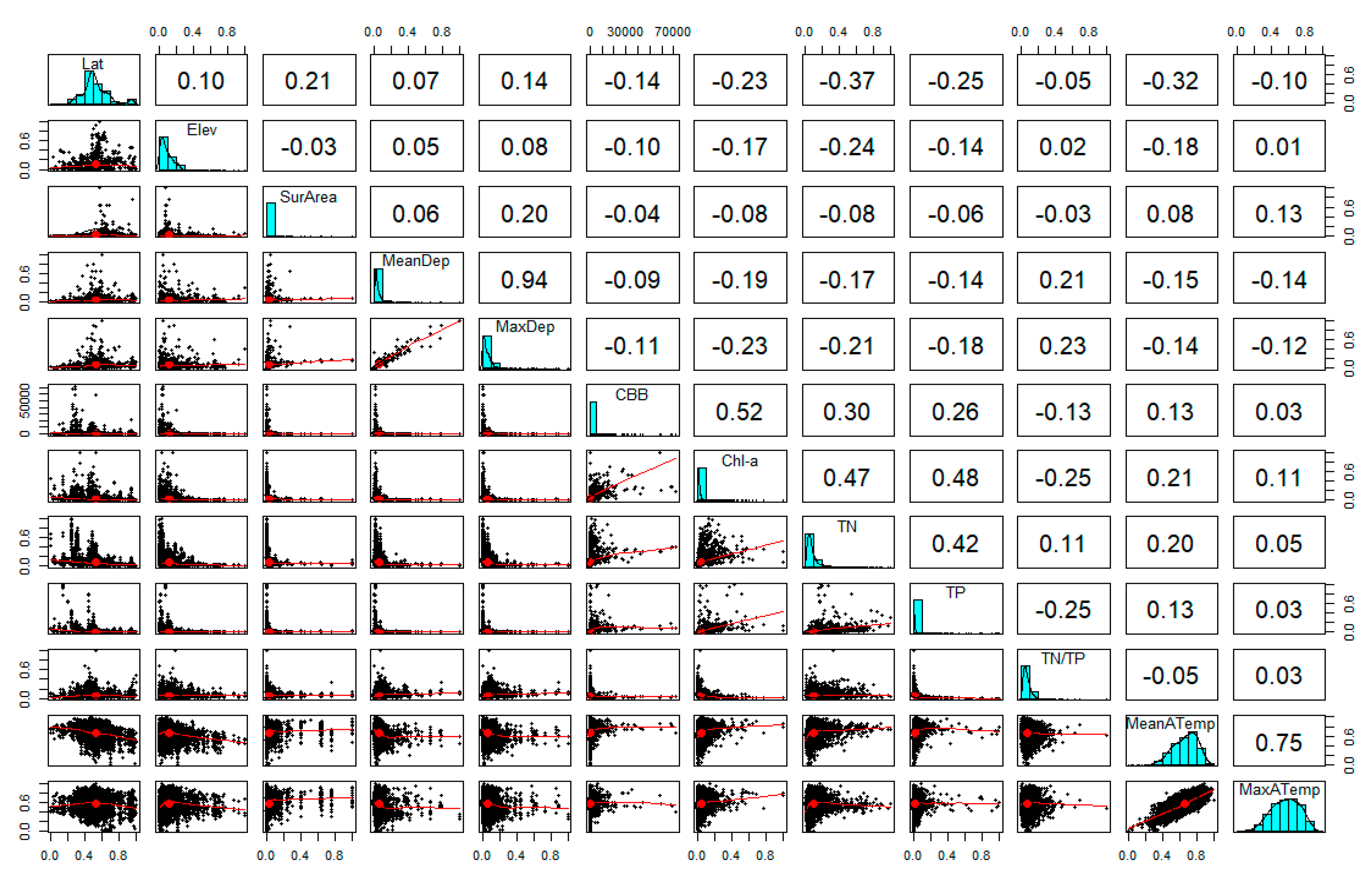
The next step was to investigate how CBB is correlated with all the candidate predictor variables (Table 2). In this regard, a correlation matrix was produced under the Pearson’s correlation coefficient method using the “psych” package [41] and the “pairs.panels” function in the programming environment R version 3.6.2 [42]. The relationships between the lake monitoring, meteorological and geomorphological data were examined by bivariate linear correlation and scatter plot smoothing, while the distribution of each variable was also investigated. In the upper right panel of Figure 4, pairwise linear correlation coefficients of the variables are illustrated, while the lower left panel displays the data as scatter plots with smooth regression curves. According to the correlation matrix in Figure 4, the explanatory variables with the highest linear correlation compared with CBB were Chl-a (r = 0.52), TN (r = 0.3) and TP (r = 0.26), which indicates that the correlation of CBB with Chl-a is the highest; in turn, the correlations of CBB with TN and TP are comparable, and even though lower than those with Chl-a, are still significant.
2.3. Stepwise Multiple Linear Regression
Stepwise multiple linear regression was applied to the whole dataset containing all the lakes, to the subset containing shallow lakes (mean depth less or equal to 3 m) and to the subset containing deep lakes (mean depth above 3 m), in order to decide which subset of predictor variables results in the best model that explains the biggest variation in CBB in each case. Even though the response of cyanobacteria to eutrophication is typically non-linear [8,43], multiple linear regression models are commonly used in predicting cyanobacteria abundance in several studies, which in many cases outperform non-linear ones in predictability and are much less complicated [17,28,44]. Furthermore, cyanobacteria abundance is far from normally distributed, which can be confirmed with the large difference between the mean and median in Table 2 and the histogram in Figure 4. The distribution has a strong positive skewness and normalization is not expected to be very helpful; as a result, assumptions underlying linear regression are violated. This is not uncommon and is tolerated because of the simplicity of multiple linear models and their satisfying predictability.
Among the predictor variables (Figure 4), max depth and max air temperature showed high collinearity with mean depth (0.94) and mean air temperature (0.75), respectively, and were omitted from the final set considered in our analysis. The final set of the predictor variables includes latitude (Lat), elevation (Elev), surface area (SurArea), mean depth (MeanDep), mean air temperature (MeanATemp), total nitrogen (TN), total phosphorus (TP), total nitrogen-to-total phosphorus ratio (TN/TP) and chlorophyll-a (Chl-a). The stepwise regression consists of iteratively adding and removing predictors, in the predictive model, in order to find the subset of variables in the dataset resulting in the best performing model; that is, a model that lowers the prediction error. In our analysis we performed backward selection or backward elimination, which starts with all predictors, iteratively removing the least contributive predictors, and stops when the model includes the predictors that are statistically significant. The Akaike Information Criterion (AIC) was used as an estimator of out-of-sample prediction error and thereby determined the best predictive model produced by the backward selection method. The performance criteria R-squared, Schwarz Bayesian Criterion (BIC) and RMSE were also calculated to compare the produced models. The dataset used in each case—the all-lakes dataset, as well as the shallow-lake and deep-lake subsets—was split in training and testing sets by the 10-fold cross-validation method in order to better assess the prediction strength of each model and to prevent overfitting. The stepwise multiple linear regression analysis was conducted in R by using the “tidyverse”, “caret”, “leaps” and “MASS” packages [45,46,47,48].
2.4. Path Analysis
Path analysis was used to decompose correlations into different pieces for interpretation of effects (e.g., how does TN, TP and MeanATemp influence CBB, directly or indirectly through Chl-a). Although cyanobacteria biomass is a component of total algal biomass, which is also measured by Chl-a, Chl-a is often used as a predictor for CBB [19]. With this type of causal modeling, we can test the cause and effect relationship of various variables that are theoretically assumed to be causally related; we can now see whether and to what degree this assumption is supported by the data. The resulting models show the causal mechanisms and the direct and indirect effects of the explanatory variables on CBB. In our case, Chl-a, TN, TP along with MeanATemp were used to construct models under various scenarios that explore all possibilities, with different combinations of direct and indirect effects of the predictor variables on CBB. All variables were chosen as the strongest predictors resulting from the literature [15], but also from the stepwise multiple regression performed. Validation of the produced models was carried out by examining the z-values and Pr (>|z|); the former is computed as the test statistic for the hypothesis test that the true corresponding regression coefficient β of variable X (Chl-a, TN, TP and MeanATemp) in predicting variable Y (CBB) is 0. The latter is the significance level of the hypothesis test, with the value of 0.05 taken as the threshold. In other words, with path analysis, we determined whether a variable matters or not, i.e., whether it has a significant relationship with variable Y. A series of permutations are explored to define the importance of each variable in predicting either Chl-a or CBB. Overall statistics, such as AIC, BIC, Root Mean Square Error of Approximation (RMSEA) and Chi-square indices are also used to assess goodness of fit in each case. All statistical calculations and representations were done in R with the “lavaan” package [49].
2.5. Machine Learning Methods
The prediction of risk to human health associated with the level of cyanobacterial abundance for recreational water use was conducted by means of a series of machine learning algorithms. The WHO [35] has published a guideline for safe practice in managing recreational water according to which there is a relatively low probability of adverse health effects when cyanobacterial cell count is less than or equal to 20,000 cells/mL; a medium or moderate probability when cyanobacterial cell count ranges from 20,000 cells/mL to 100,000 cells/mL and a high probability when that cell count is above 100,000 cells/mL. Since the dataset includes concentrations and not cell counts, the latter had to be transformed to cyanobacterial biomass, to enable the classification of data in the WHO data ranges. Considering that the mean cyanobacterial cell weighs approximately 10−7 mg we converted cyanobacterial cell density to biomass [43]. Table 3 presents the three risk categories for recreational use, according to cyanobacteria biomass.
By matching CBB to the three risk categories, the continuous dependent variable was transformed to a categorical one representing three levels—low, moderate and high. Subsequently, the whole dataset was divided into training and testing subsets following an 80% to 20% ratio, respectively. Four machine learning algorithms were applied in order to determine which algorithm has better efficiency in predicting the risk categories with the input parameters being the eleven explanatory variables presented in Table 2 and in the correlation matrix in Figure 4. Since machine learning algorithms are based on the simple idea of “the wisdom of the crowd” and the aggregation of the results of multiple predictors gives better predictions, all explanatory variables were used [50]. The machine learning methods used were Decision Tree (DT), K-Nearest Neighbors (k-NN), Support-vector Machine (SVM) and Random Forest (RF), which are briefly described as follows:
- DT is a supervised machine learning technique for inducing a decision tree from training data. A decision tree, also referred to as a classification tree, is a flowchart-like diagram that shows the various outcomes from a series of decisions. Practically, it is the mapping of observations about an item to conclusions about its target value [51].
- k-NN is a relatively simple approach to classification that is completely nonparametric. Given a point x0 that one wishes to classify into one of the K groups, the algorithm finds the k observed data points that are nearest to x0. The classification rule is to assign x0 to the population that has the most observed data points out of the k-nearest neighbors. Points for which there is no majority are either classified to one of the majority populations at random or left unclassified [52].
- SVM is an algorithm that classifies data by determining the optimal hyperplane that separates observations according to their class labels. The central concept of this method is to accommodate classes that are separable by linear and non-linear class boundaries [53].
- RF is a classifier algorithm that evolved from decision trees. It collects the classifications and chooses the most voted prediction as the result. RFs sample data from the original dataset and a subset of features is randomly selected from the optional features to grow the tree at each node. The strength of the RFs relies on the capability to enable a large number of weak or weakly correlated classifiers to form a strong classifier [54].
3. Results and Discussion
3.1. Identifying Variables Explaining CBB Variation
By applying stepwise linear regression with backward elimination to the original dataset and to the subsets of shallow and deep lakes with AIC as performance indicator, the following results were obtained. Regarding the all-lakes dataset, the best overall model structure that explains the most variation in CBB is the one including Chl-a and TN as predictors (R2 = 0.33). Although Chl-a, as a single predictor, showed a proportional ability to capture the variation in CBB (R2 = 0.33), when Chl-a is combined with TN, the overall performance of the model exceeds that of Chl-a, as indicated by the performance criteria summarized in Table 4 (BIC, AIC and RMSE). In the subgroup of shallow lakes, stepwise regression resulted in a four-variable linear model, including Chl-a, TN, MeanDep and TN/TP as best predictors according to the AIC criterion (R2 = 0.27). Similarly to the all lakes dataset, although the best single-variable linear model (Chl-a) and the best two-variable (Chl-a and TN) and three-variable models (Chl-a, TN and MeanDep) had similar R-square values, their overall performance was weaker compared to the four-variable model. Furthermore, the predictive power of the best linear model for the subgroup of shallow lakes was weaker compared to the model that represents the subgroup of the original dataset for all lakes. Finally, in the subgroup of deep lakes, the model that better predicted the variation of the CBB included Chl-a, TN and TN/TP (R2 = 0.44). The two-variable (Chl-a and TN/TP) and single-variable (Chl-a) best models in this case, showed lower R2 values and weaker predictive performance criteria. In general, the linear models predicting CBB in deep lakes exhibited a remarkable improvement against the all-lakes and shallow-lakes models. Although it is somewhat surprising, since cyano-blooms is a more common problem in shallow lakes, this finding is justified by the fact that prediction is more difficult in shallow lakes because of more fluctuating conditions. However, similar results, where modelling efficacy improves in deep lakes, can be found in other studies [17,28]. In Table 4, the best univariate and multivariate models as well as their performance indicators are summarized. Our analysis shows that using linear models to predict CBB concentration from biological and physical–chemical lake variables has a relatively low reliability, which is reflected by the low R2 values. To deal with this, we explored the possibility of producing more reliable results by predicting health risk levels, instead of concentrations. This is presented in Section 3.3.
3.2. Describing Dependent Relationships among Variables
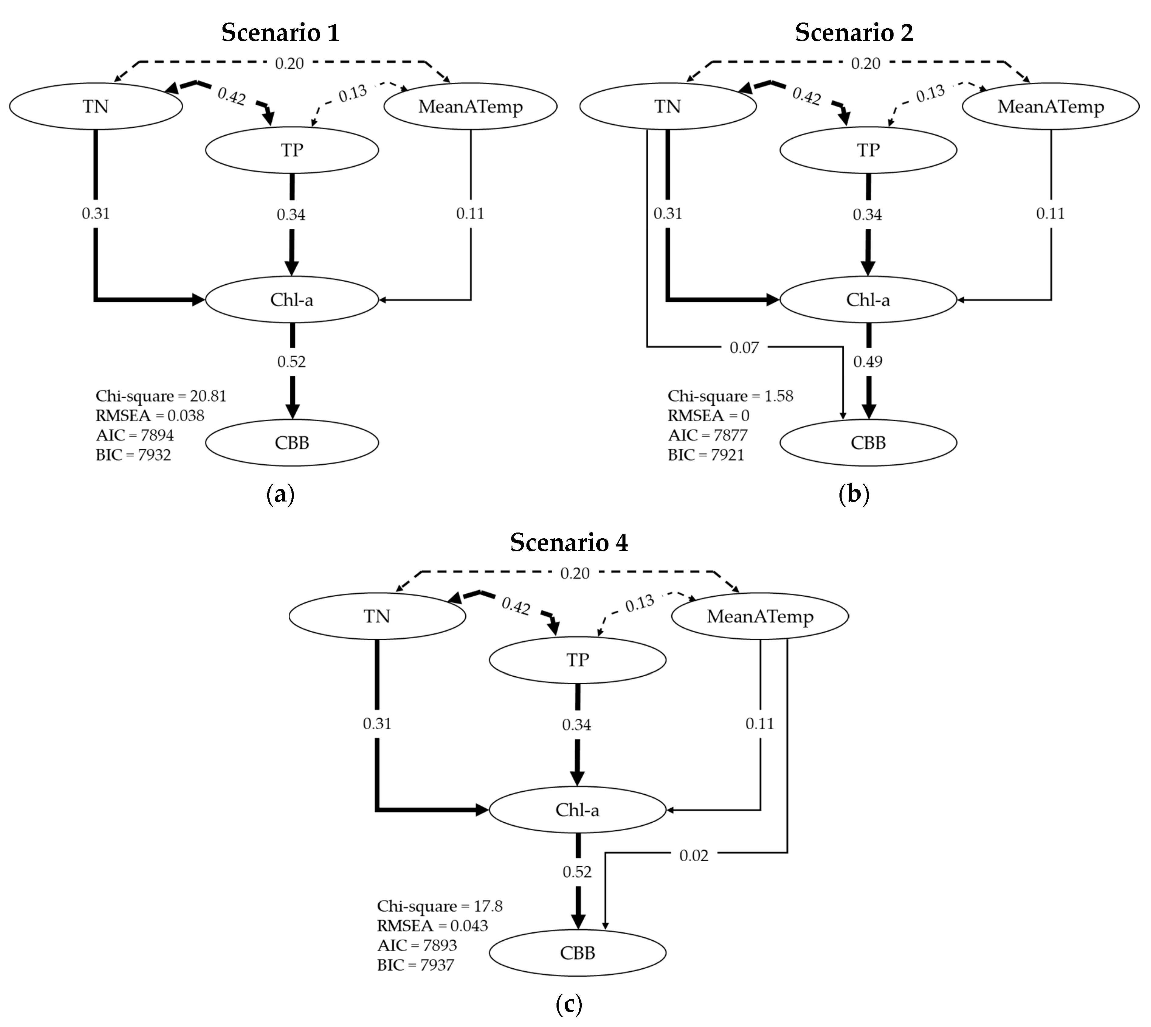
Path analysis was performed for four different competing scenarios, in order to explore how strongly certain variables (TN, TP and MeanATemp) act in mediating the relationship between Chl-a and CBB. We explore how the model regresses Chl-a on TN, TP and MeanATemp and how the model directly regresses CBB on Chl-a, TN, TP and MeanATemp. Results of the path analysis, as produced from the R studio package, are shown in Table 5. In Scenario (1), we explore how the model regresses Chl-a on TN, TP and MeanATemp. For all three variables, we see that z-value > 2 and Pr (>|z|) < 0.05, so they are all significant in determining Chl-a. We also explore how CBB is regressed on Chl-a and again we see that Chl-a is significant. In Scenario (2) and having secured that TN, TP and MeanATemp are significant, we further explore how the model regresses CBB directly on TN (in addition to Chl-a). Results show that TN is indeed significant. Similarly, in Scenarios (3) and (4) we explore sequentially the significance of TP and MeanATemp, respectively, in influencing CBB directly. In Scenario (3), results show that TP is not significant, since the z-value is less than 2 and Pr (>|z|) > 0.05. In Scenario 4, the z-value (1.736) is close to 2 and Pr (>|z|) (0.083) is close to 0.05, indicating a marginal significance of MeanATemp in influencing CBB directly.
In Figure 5, we see a schematic representation that shows the standardized path coefficients for Scenarios (1), (2) and (4), while other statistics, such as Chi-square, RMSEA, AIC and BIC are shown as well. According to the statistics, Scenario (2) is the best, since the statistics are the lowest. The dashed lines depict the correlation coefficients between the two variables they connect (repeated from Figure 4). Our path analysis shows that TP is not included in the variables that are significant for CBB, while TN is included. This fact indicates a potential nitrogen limitation, meaning that even when TP increases, it stops being significant since CBB is nitrogen dependent; similar results are reported in the literature [60]. This is especially true since the lakes in our dataset seem to be highly P enriched (see Table 2).
3.3. Evaluating the Performance of the Machine Learning Methods
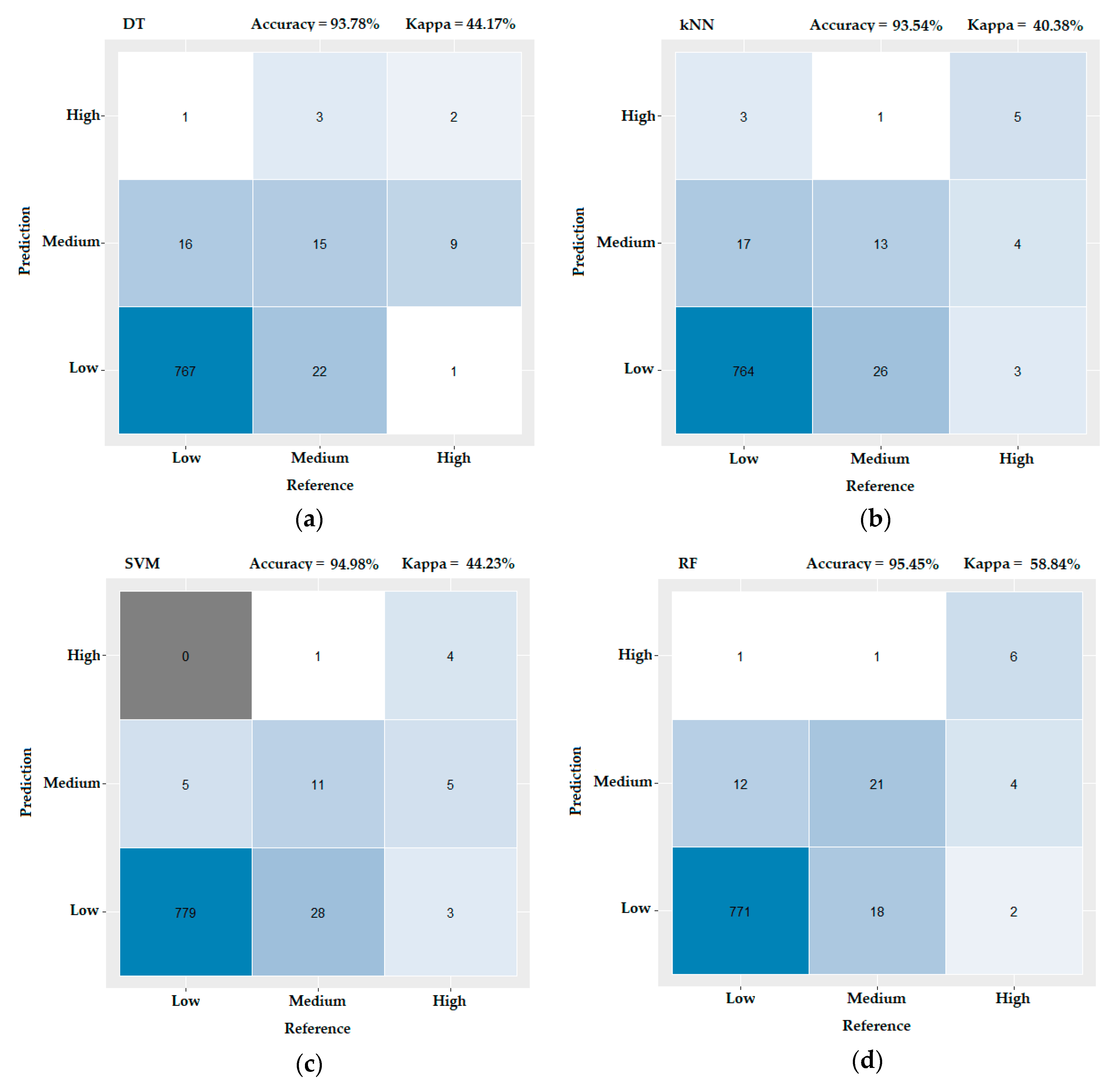
A series of machine learning algorithms were used to compare their predictive potential towards identifying the risk to human health associated with CBB level for recreational activities. In Figure 6, confusion matrices and the corresponding performance indices for algorithms DT, k-NN, SVM and RF are presented. These matrices depict the number of instances that the predicted values of the CBB risk levels matched the reference (actual) risk levels or failed to predict the risk levels correctly. The instances presented on the diagonal are all True Positives, since the algorithm prediction matches the actual classification (what is predicted as a low is actually a low, a predicted medium is a medium, etc.) In Figure 6a, this number is 784. The sum of the actual instances that are not predicted correctly are the False Negatives; in Figure 6a, the False Negatives are 17 for “Low”, 25 for “Medium” and 10 for “High”, and they are calculated as the sum of each column minus the True Positives. False Positives are the instances that are predicted falsely and are the sum of each row minus the True Positives. In Figure 6a, the False Positives are 23 for “Low”, 25 for “Medium” and 4 for “High”. Finally, the True Negatives for a certain class are those instances that do not belong in that class (either predicted or reference), so in Figure 6a, we have 29 True Negatives for “Low”, 771 True Negatives for “Medium” and 820 True Negatives for “High”.
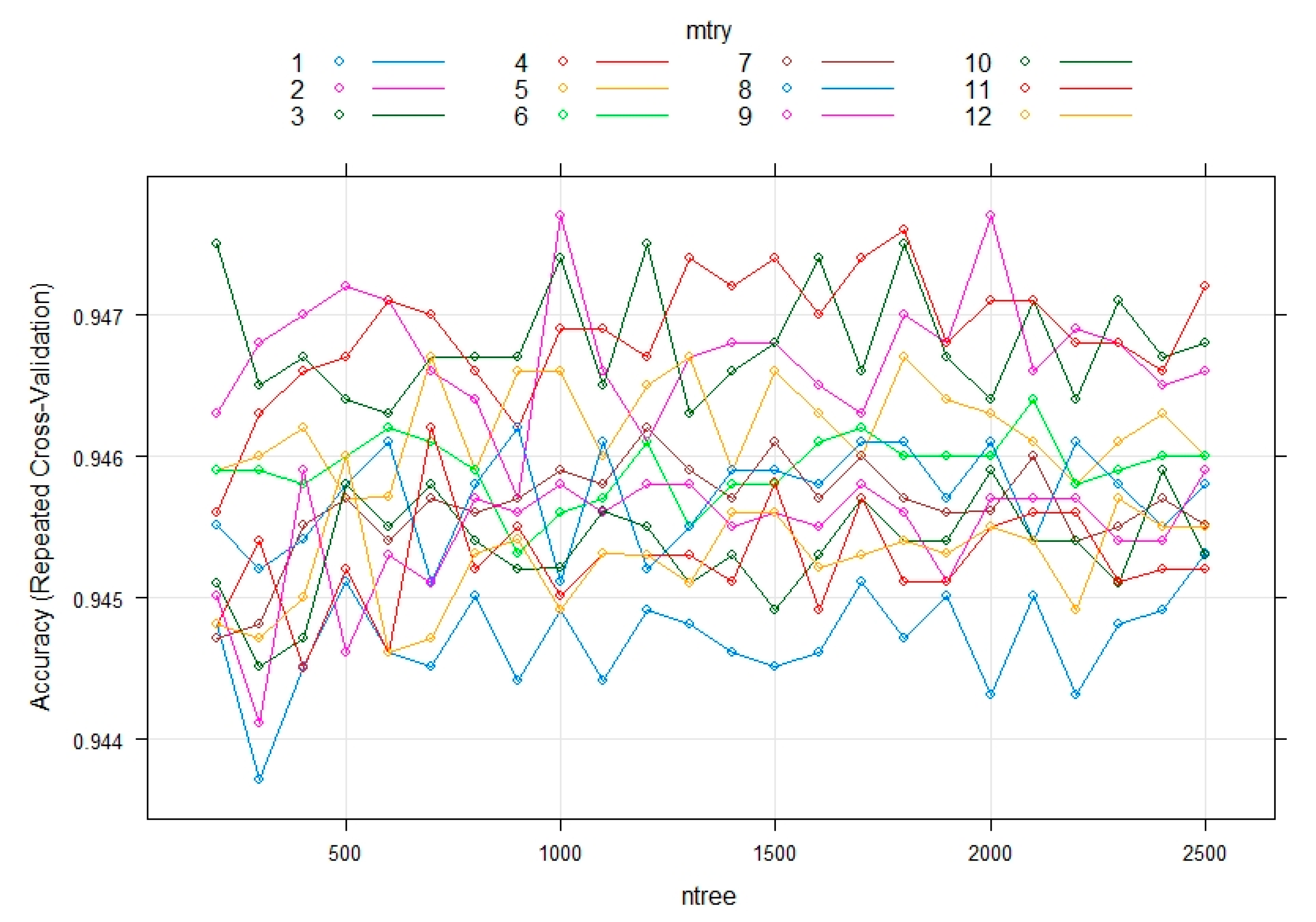
The overall metrics we use to assess the performance of these algorithms are “Accuracy” and “Kappa”—a single value per confusion matrix is calculated for these two variables. Accuracy is defined as the ratio of all True Positives of the matrix divided by the sum of all instances in the dataset and it expresses the ability of the model to correctly identify Low, Medium and High instances. Kappa statistics considers the fact that some of the correct predictions may be identified as such by chance, so it adjusts the reported model accuracy by considering the effect of randomness in correct predictions [61]. Comparing the four implemented machine learning algorithms, in Figure 6 we see that both for accuracy and Kappa statistics, the RF performs best. Thus, according to the results, RF has the highest metrics (Accuracy = 95.45% and Kappa = 58.84%) and was selected for tuning its parameters, in order to further improve its performance. The tuning procedure was conducted in R by using the packages “randomForest”, “mlbench” and “caret” [46,59,62]. We applied the grid search method under 10-fold repeated cross validation, in order to search for the best combination of parameters, namely the functions “mtry” and “ntree”. Mtry is the number of variables randomly sampled as candidates for each split, while ntree is the number of trees to grow [63]. After exhaustively checking all parameters and combinations with the grid search method, we concluded that the highest levels of accuracy are achieved for a mtry equal to 2 and for ntree taking the values of 1000 and 2000. Results of this analysis is shown in Figure 7: Each colored line represents the fluctuation of accuracy (y-axis) when different ntree values (x-axis) are applied on each of the possible values for mtry (colored lines). We focus on the highest accuracy, i.e., which one of the colored lines achieves the highest y value (this is true for the purple line that has the highest peaks and corresponds to mtry = 2, according to the legend in Figure 7). For this line, the highest peaks correspond to ntree (x-axis) values of 1000 and 2000; thus, these are the chosen model parameters that optimize accuracy.
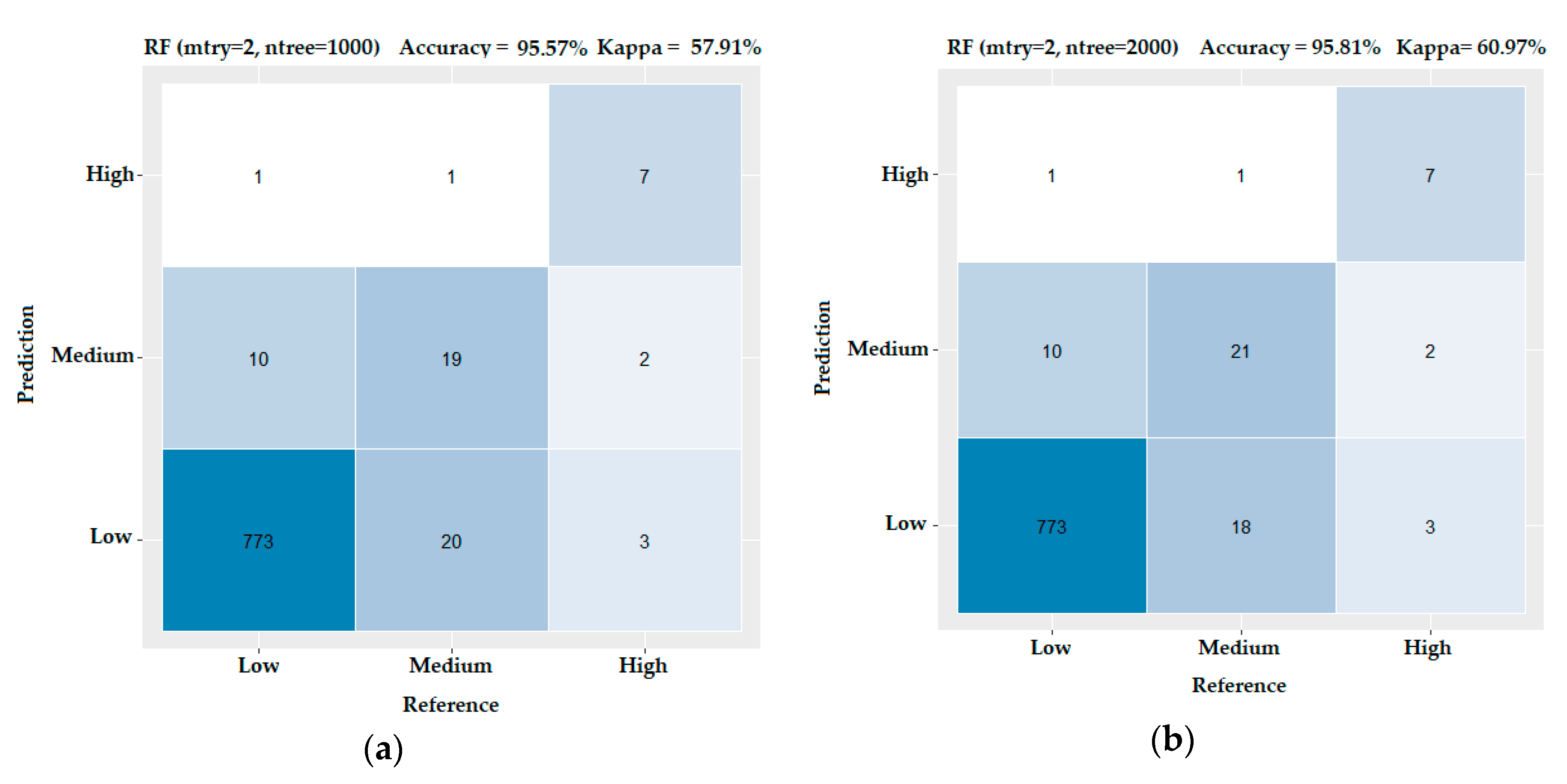
In order to check the performance of RF under these two prevailing combinations of parameters on the dataset, we produced two confusion matrices—one for mtry = 2 and ntree = 1000 and another for mtry = 2 and ntree = 2000. As we show in Figure 8, the best performance was achieved for mtry = 2 and ntree = 2000 (Accuracy = 95.81% and Kappa = 60.97%) (Figure 8b). According to [64], a model is considered to produce accurate predictions when Kappa exceeds 60%, which in our case is succeeded.
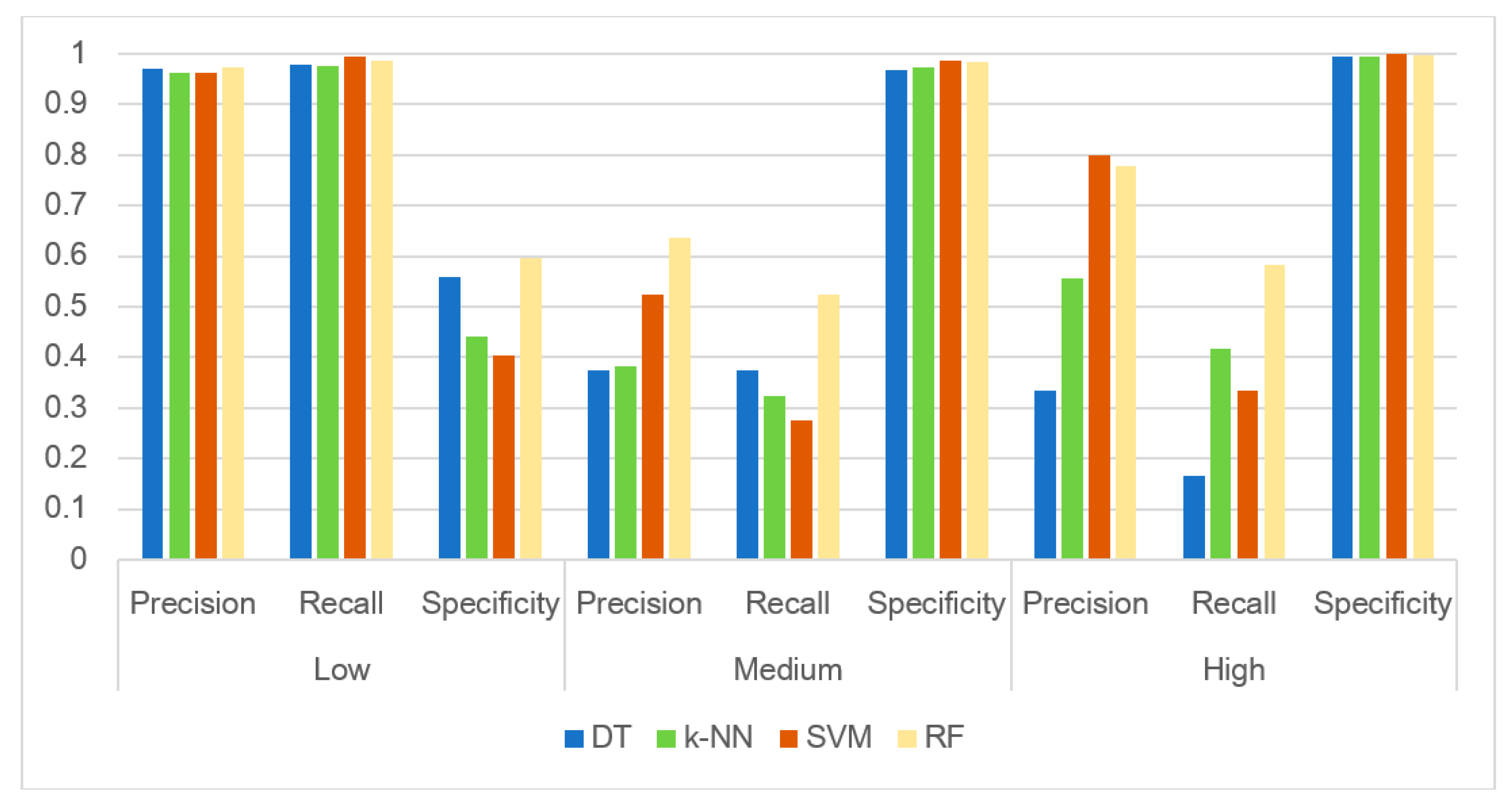
To further analyze the modeling results, we compared in detail the performance of the four algorithms by using three metrics: precision, recall and specificity [61]. Precision is defined for each class (Low, Medium and High) as the ratio of True Positives by the sum of True Positives and False Positives for that class. In Figure 9, we see that precision is the highest for the Low class, most probably due to the large number of observations in that class; it approaches 1, which means that given many observations, all algorithms predict with great precision. In the High class, where we have the least observations, precision is close to 80% for SVM and RF, with SVM giving slightly better results. It is weakest in the Medium class, with RF still giving the best results. It should be noted that precision becomes important when the cost of False Positives is high. In our case, this means the cost of predicting that CBB concentrations are High (Low) when they are actually medium or Low (High). The former case of having high CBB concentrations being falsely predicted as low, which is an undesirable scenario in terms of public health, has a precision of about 80%. Given the very small number of observations in the High category, this is a strong outcome in terms of the capacity of the optimized RF scheme to predict events with excellent precision.
Recall is calculated as the ratio of True Positives by the sum of True Positives and False Negatives, which is the ratio of True Positives by Total Actual Positives. Recall calculates how many of the actual Lows (Highs) the algorithm captures through labeling them as Lows (Highs). We see that, again, in the Low class where we have many observations, recall is almost 1. In the Medium and High classes, recall is lower, but the optimized RF algorithm performs significantly higher in all classes. The recall metric becomes important when there is a high cost associated with False Negatives; in our case, a False Negative would mean that a High risk level is falsely predicted by the model as either Medium or Low. In terms of protecting public health, this would have a really high cost and authorities want to have the right tools to avoid such situations. In the High and Medium classes, where we have few data, we see that recall values are between 50% and 60%, which indicates that the instances that the model will predict False Negatives is relatively high. The fact that the numbers are close to 1 for the Low class, in which we have many observations, signifies the importance of the number of data observations.
Finally, specificity is the true negative rate and is calculated as the number of correct negative predictions (for the Low class, this is the sum of observations that are actually Medium and High minus the ones that are falsely predicted as Low) divided by the total number of Negatives (True Negatives + False Positives—for the Low class, this includes all observations that are actually Medium and High). This metric is an indication of how good the model is at avoiding false alarms. So, when we report High (Medium), we have a probability of almost 100% to avoid false alarms, which means that the CBB concentrations are indeed High (Medium). When the Low class is reported, then the results show that there is an average probability for avoiding false alarms, which means that it is possible that a false alarm is created. This possibility for a false alarm is the highest in the Low class, which is not ideal, since it means that we may report Low but actual risk levels may indeed be Medium or High. Specificity would improve if we had more data in the Medium of High class. The fact that our dataset is very unbalanced, with many more observations in the Low class than in the other two classes, creates the corresponding imbalance in our results, with excellent predictions for the Low class and less accurate predictions in the other two classes. This of course is an important finding, since it indicates that the multitude of observations is critical in obtaining solid predictions. When authorities have the capacity to obtain such observations through online real-time monitoring, for example, resulting in large datasets, they can count on machine learning algorithms for reliable results that will assist them in taking informed decisions that protect public health and wellbeing.
4. Conclusions
This article explores the complexity of mechanisms that determine cyanobacteria abundance in lake ecosystems through stepwise multiple linear regression and a series of machine learning methods, namely Decision Tree, K-Nearest Neighbors, Support-vector Machine and Random Forest. The analysis advocates the multifactorial nature of cyanobacteria response to environmental conditions. Path analysis on the direct–indirect and cause–effect relationships of the stressors reveals that when Chl-a is included as one of the predictors of CBB, TN significantly affects CBB, air temperature only marginally affects its abundance, while TP is found to be not significant. Multiple linear regression analysis reports R2 values that are in line with values reported by previous studies, even though they are relatively low (R2 = 0.33 for all lakes, R2 = 0.27 for shallow and R2 = 0.44 for deep lakes). When differentiating the predicting approach and translating CBB to risk categories associated with impacts on public health by the recreational use of lakes, predictive ability was fundamentally improved. Machine learning methods and especially Random Forest proved to be a reliable and highly accurate tool towards the categorization of lakes to risk levels, achieving model accuracy levels as high as 95.81% after having optimized the parameters of the algorithm. Confusion matrix analysis resulted in the quantification of the probability of false alarms for the three different risk levels. Focusing on current machine learning techniques to assess cyanobacteria risk levels to human health can give crucial insights to water managers and consequently raise public awareness in a timely manner as to when the lake water is inappropriate to serve recreational uses.
Author Contributions
Conceptualization: N.M.; methodology: N.M.; software: N.M.; validation: N.M., C.L.; formal analysis: N.M. and C.L.; resources: C.L.; data curation: S.J.M.; writing—original draft preparation: N.M.; writing—review and editing: C.L. and S.J.M.; visualization: N.M.; supervision: C.L.; project administration: C.L., funding acquisition: C.L. All authors have read and agreed to the published version of the manuscript.
Funding
The work described in this paper has been conducted within the project WATER4CITIES—Holistic Surface Water and Groundwater Management for Sustainable Cities—which is implemented in the framework of the EU Horizon2020 Program, Grant Agreement Number 734409. This paper and the content included in it do not represent the opinion of the European Union, and the European Union is not responsible for any use that might be made of its content.
Acknowledgments
We thank the following organisations and persons for making phytoplankton and environmental data available through the WISER Central Database. UK: Environment Agency England & Wales (EA) and Scottish Environment Protection Agency (SEPA) (Geoff Phillips, Lawrence Carvalho); Norway: Norwegian Institute for Water Research (NIVA) (Anne Lyche Solheim, Birger Skjelbred); Sweden: Swedish University of Agricultural Sciences (SLU) (Stina Drakare); Finland: Finnish Environment Institute (SYKE) (Marko Järvinen); Denmark: Aarhus University (Martin Søndergaard, Ivan Karottki); Lithuania: Environmental Protection Agency Lithuania (AAA) (Audrone Pumputyte).
Conflicts of Interest
The authors declare no conflict of interest.
References
- Carmichael, W. A world overview—One-hundred-twenty-seven years of research on toxic cyanobacteria—Where do we go from here? In Cyanobacterial Harmful Algal Blooms: State of the Science and Research Needs; Hudnell, H.K., Ed.; Springer: New York, NY, USA, 2008; Volume 619, pp. 105–125. [Google Scholar]
- Paerl, H.W.; Huisman, J. Blooms like it hot. Science 2008, 320, 57–58. [Google Scholar] [CrossRef] [Green Version]
- O’Neil, J.M.; Davis, T.W.; Burford, M.A.; Gobler, C.J. The rise of harmful cyanobacteria blooms: The potential roles of eutrophication and climate change. Harmful Algae 2012, 14, 313–334. [Google Scholar] [CrossRef]
- Carmichael, W.W.; Boyer, G.L. Health impacts from cyanobacteria harmful algae blooms: Implications for the North American Great Lakes. Harmful Algae 2016, 54, 194–212. [Google Scholar] [CrossRef] [PubMed]
- Mellios, N.; Papadimitriou, T.; Laspidou, C. Predictive modeling of microcystin concentrations in a hypertrophic lake by means of Adaptive Neuro Fuzzy Inference System (ANFIS). Eur. Water 2016, 55, 91–103. [Google Scholar]
- Lévesque, B.; Gervais, M.-C.; Chevalier, P.; Gauvin, D.; Anassour-Laouan-Sidi, E.; Gingras, S.; Fortin, N.; Brisson, G.; Greer, C.; Bird, D. Prospective study of acute health effects in relation to exposure to cyanobacteria. Sci. Total Environ. 2014, 466, 397–403. [Google Scholar] [CrossRef]
- Hamilton, D.P.; Wood, S.A.; Dietrich, D.R.; Puddick, J. Costs of harmful blooms of freshwater cyanobacteria. In Cyanobacteria: An Economic Perspective; Sharma, N.K., Rai, A.K., Stal, L.J., Eds.; John Wiley & Sons: Chichester, UK, 2013; Volume 1, pp. 245–256. [Google Scholar]
- Solheim, A.L.; Rekolainen, S.; Moe, S.J.; Carvalho, L.; Philips, G.; Ptacnik, R.; Penning, W.E.; Tóth, L.G.; O’Toole, C.; Schartau, A.K.; et al. Ecological threshold responses in European lakes and their applicability for the Water Framework Directive (WFD) implementation: Synthesis of lakes results from the REBECCA project. Aquat. Ecol. 2008, 42, 317–334. [Google Scholar] [CrossRef]
- Francis, G. Poisonous Australian Lake. Nature 1878, 18, 11–12. [Google Scholar] [CrossRef] [Green Version]
- Carpenter, S.R.; Stanley, E.H.; Vander Zanden, M.J. State of the world’s freshwater ecosystems: Physical, chemical, and biological changes. Annu. Rev. Environ. Resour. 2011, 36, 75–99. [Google Scholar] [CrossRef] [Green Version]
- Elliott, J.A. The seasonal sensitivity of cyanobacteria and other phytoplankton to changes in flushing rate and water temperature. Glob. Chang. Biol. 2010, 16, 864–876. [Google Scholar] [CrossRef]
- Paerl, H.W.; Otten, T.G. Harmful cyanobacterial blooms: Causes, consequences, and controls. Microb. Ecol. 2013, 65, 995–1010. [Google Scholar] [CrossRef]
- Wells, M.L.; Trainer, V.L.; Smayda, T.J.; Karlson, B.S.O.; Trick, C.G.; Kudela, R.M.; Ishikawa, A.; Bernard, S.; Wulff, A.; Anderson, D.M.; et al. Harmful algal blooms and climate change: Learning from the past and present to forecast the future. Harmful Algae 2015, 49, 68–93. [Google Scholar] [CrossRef] [PubMed] [Green Version]
- Laspidou, C.; Kofinas, D.; Mellios, N.; Latinopoulos, D.; Papadimitriou, T. Investigation of factors affecting the trophic state of a shallow Mediterranean reconstructed lake. Ecol. Eng. 2017, 103, 154–163. [Google Scholar] [CrossRef]
- Mellios, N.; Kofinas, D.; Laspidou, C.; Papadimitriou, T. Mathematical modeling of trophic state and nutrient flows of Lake Karla using the PCLake model. Environ. Process. 2015, 2, 85–100. [Google Scholar] [CrossRef] [Green Version]
- Richardson, J.; Feuchtmayr, H.; Miller, C.; Hunter, P.D.; Maberly, S.C.; Carvalho, L. Response of cyanobacteria and phytoplankton abundance to warming, extreme rainfall events and nutrient enrichment. Glob. Chang. Biol. 2019, 25, 3365–3380. [Google Scholar] [CrossRef] [Green Version]
- Beaulieu, M.; Pick, F.; Gregory-Eaves, I. Nutrients and water temperature are significant predictors of cyanobacterial biomass in a 1147 lakes data set. Limnol. Oceanogr. 2013, 58, 1736–1746. [Google Scholar] [CrossRef]
- Moe, S.J.; Couture, R.M.; Haande, S.; Lyche Solheim, A.; Jackson-Blake, L. Predicting lake quality for the next generation: Impacts of catchment management and climatic factors in a probabilistic model framework. Water 2019, 11, 1767. [Google Scholar] [CrossRef] [Green Version]
- Romo, S.; Soria, J.; Fernandez, F.; Ouahid, Y.; Baron-Sola, A. Water residence time and the dynamics of toxic cyanobacteria. Freshw. Biol. 2013, 58, 513–522. [Google Scholar] [CrossRef]
- Paerl, H.W.; Fulton, R.S.; Moisander, P.H.; Dyble, J. Harmful freshwater algal blooms, with an emphasis on cyanobacteria. Sci. World J. 2001, 1, 76–113. [Google Scholar] [CrossRef]
- Wood, S.A.; Prentice, M.J.; Smith, K.; Hamilton, D.P. Low dissolved inorganic nitrogen and increased heterocyte frequency: Precursors to Anabaena planktonica blooms in a temperate, eutrophic reservoir. J. Plankton Res. 2010, 32, 1315–1325. [Google Scholar] [CrossRef] [Green Version]
- Noges, T.; Laugaste, R.; Noges, P.; Tonno, I. Critical N: P ratio for cyanobacteria and N 2-fixing species in the large shallow temperate lakes Peipsi and Võrtsjärv, North-East Europe. Hydrobiologia 2008, 599, 77–86. [Google Scholar] [CrossRef]
- Havens, K.E.; Phlips, E.J.; Cichra, M.F.; Li, B.L. Light availability as a possible regulator of cyanobacteria species composition in a shallow subtropical lake. Freshw. Biol. 1998, 39, 547–556. [Google Scholar] [CrossRef]
- Scheffer, M.; Rinaldi, S.; Gragnani, A.; Mur, L.R.; Van Nes, E.H. On the dominance of filamentous cyanobacteria in shallow, turbid lakes. Ecology 1997, 78, 272–282. [Google Scholar] [CrossRef]
- Carey, C.C.; Ibelings, B.W.; Hoffmann, E.P.; Hamilton, D.P.; Brookes, J.D. Eco-physiological adaptations that favour freshwater cyanobacteria in a changing climate. Water Res. 2012, 46, 1394–1407. [Google Scholar] [CrossRef] [PubMed]
- Brookes, J.D.; Carey, C.C. Resilience to blooms. Science 2011, 334, 46–47. [Google Scholar] [CrossRef]
- Kosten, S.; Huszar, V.L.; Bécares, E.; Costa, L.S.; Van Donk, E.; Hansson, L.A.; Jeppesen, E.; Kruk, C.; Lacerot, G.; Mazzeo, N.; et al. Warmer climates boost cyanobacterial dominance in shallow lakes. Glob. Chang. Biol. 2012, 18, 118–126. [Google Scholar] [CrossRef]
- Richardson, J.; Miller, C.; Maberly, S.C.; Taylor, P.; Globevnik, L.; Hunter, P.; Jeppesen, E.; Mischke, U.; Moe, S.J.; Pasztaleniec, A.; et al. Effects of multiple stressors on cyanobacteria abundance vary with lake type. Glob. Chang. Biol. 2018, 24, 5044–5055. [Google Scholar] [CrossRef] [Green Version]
- Psilovikos, A. Water Resources; Tziolas: Thessaloniki, Greece, 2020; ISBN 978-960-602-0. (In Greek) [Google Scholar]
- Karamoutsou, L.; Psilovikos, A. The use of Artificial Neural Network in Water Quality Prediction in Lake Kastoria, Greece. In Proceedings of the 14th Conference of the Hellenic hydrotechnical Association (HHA), Volos, Greece, 16–17 May 2019; pp. 882–889. [Google Scholar]
- Rigosi, A.; Carey, C.C.; Ibelings, B.W.; Brookes, J.D. The interaction between climate warming and eutrophication to promote cyanobacteria is dependent on trophic state and varies among taxa. Limnol. Oceanogr. 2014, 59, 99–114. [Google Scholar] [CrossRef] [Green Version]
- Taranu, Z.E.; Zurawell, R.W.; Pick, F.; Gregory-Eaves, I. Predicting cyanobacterial dynamics in the face of global change: The importance of scale and environmental context. Glob. Chang. Biol. 2012, 18, 3477–3490. [Google Scholar] [CrossRef]
- Wei, B.; Sugiura, N.; Maekawa, T. Use of artificial neural network in the prediction of algal blooms. Water Res. 2001, 35, 2022–2028. [Google Scholar] [CrossRef]
- Recknagel, F.; French, M.; Harkonen, P.; Yabunaka, K.I. Artificial neural network approach for modelling and prediction of algal blooms. Ecol. Model. 1997, 96, 11–28. [Google Scholar] [CrossRef]
- World Health Organization. Guidelines for Safe Recreational Waters: Coastal and Fresh Waters; Chapter 8; WHO Publishing: Geneva, Switzerland, 2003; Volume 1, pp. 136–158. [Google Scholar]
- Bláha, L.; Babica, P.; Maršálek, B. Toxins produced in cyanobacterial water blooms-toxicity and risks. Interdiscip. Toxicol. 2009, 2, 36–41. [Google Scholar] [CrossRef] [PubMed] [Green Version]
- Moe, S.J.; Schmidt-Kloiber, A.; Dudley, B.J.; Hering, D. The WISER way of organising ecological data from European rivers, lakes, transitional and coastal waters. Hydrobiologia 2013, 704, 11–28. [Google Scholar] [CrossRef] [Green Version]
- Hering, D.; Borja, A.; Carvalho, L.; Feld, C.K. Assessment and recovery of European water bodies: Key messages from the WISER project. Hydrobiologia 2013, 704, 1–9. [Google Scholar] [CrossRef]
- Schmidt-Kloiber, A.; Moe, S.J.; Dudley, B.; Strackbein, J.; Vogl, R. The WISER metadatabase: The key to more than 100 ecological datasets from European rivers, lakes and coastal waters. Hydrobiologia 2013, 704, 29–38. [Google Scholar] [CrossRef] [Green Version]
- Jordan, M.I.; Mitchell, T.M. Machine learning: Trends, perspectives, and prospects. Science 2015, 349, 255–260. [Google Scholar] [CrossRef] [PubMed]
- Revelle, W. psych: Procedures for Personality and Psychological Research, Northwestern University, Evanston, Illinois, USA. 2017. Available online: https://CRAN.R-project.org/package=psych/ (accessed on 25 November 2019).
- Team, R.C. R: A Language and Environment for Statistical Computing. R Foundation for Statistical Computing, Vienna, Austria. Available online: https://www.R-project.org/ (accessed on 20 November 2019).
- Carvalho, L.; McDonald, C.; De Hoyos, C.; Mischke, U.; Phillips, G.; Borics, G.; Poikane, S.; Skjelbred, B.; Solheim, A.L.; Van Wichelen, J.; et al. Sustaining recreational quality of European lakes: Minimizing the health risks from algal blooms through phosphorus control. J. Appl. Ecol. 2013, 50, 315–323. [Google Scholar] [CrossRef] [Green Version]
- Ghaffar, S.; Stevenson, R.J.; Khan, Z. Cyanobacteria Dominance in Lakes and Evaluation of Its Predictors: A Study of Southern Appalachians Ecoregion, USA. In MATEC Web of Conferences. EDP Sci. 2016, 60, 02001. [Google Scholar]
- Wickham, H.; Averick, M.; Bryan, J.; Chang, W.; D’Agostino McGowan, L.; François, R.; Grolemund, G.; Hayes, A.; Henry, L.; Hester, J.; et al. Welcome to the Tidyverse. J. Open Source Softw. 2019, 4, 1686. [Google Scholar] [CrossRef]
- Kuhn, M.; Wing, J.; Wenston, S.; Williams, A.; Keefer, C.; Engelhardt, A.; Cooper, T.; Mayer, Z.; Kenkel, B.; Team, R.C.; et al. Caret: Classification and regression training. R Package Version 2016, 6, 78. [Google Scholar]
- Lumley, T.; Miller, A. Leaps: Regression subset selection. R Package Vesion 2009, 2, 2366. [Google Scholar]
- Venables, B.D.; Ripley, W.N. Modern Applied Statistics with S, 4th ed.; Springer: New York, NY, USA, 2008; pp. 1–496. [Google Scholar]
- Rosseel, Y. Lavaan: An R package for structural equation modeling and more. Version 0.5–12 (BETA). J. Stat. Softw. 2012, 48, 1–36. [Google Scholar] [CrossRef] [Green Version]
- Rokach, L. Ensemble-based classifiers. Artif. Intell. Rev. 2010, 33, 1–39. [Google Scholar] [CrossRef]
- Rokach, L.; Maimon, O. Top-down induction of decision trees classifiers-a survey. IEEE Trans. Syst. ManCybern. Part C 2005, 35, 476–487. [Google Scholar] [CrossRef] [Green Version]
- Neath, R.C.; Johnson, M.S. Discrimination and Classification. In International Encyclopedia of Education, 3rd ed.; Baker, E., McGaw, B., Peterson, P., Eds.; Elsevier Ltd.: London, UK, 2010; Volume 1, pp. 135–141. [Google Scholar]
- Hsu, C.W.; Lin, C.J. A comparison of methods for multiclass support vector machines. IEEE Trans. Neural Netw. 2002, 13, 415–425. [Google Scholar] [PubMed] [Green Version]
- Mao, W.; Wang, F.Y. Cultural Modeling for Behavior Analysis and Prediction. In New Advances in Intelligence and Security Informatics, 1st ed.; Academic Press: Waltham, MA, USA, 2012; pp. 91–102. [Google Scholar]
- Wickham, H. ggplot2: Elegant Graphics for Data Analysis, 1st ed.; Springer: New York, NY, USA, 2016. [Google Scholar]
- Therneau, T.; Atkinson, B.; Ripley, B. Rpart: Recursive Partitioning and Regression Trees, R Package Version 4.1-13. 2018. Available online: https://CRAN.R-project.org/package=rpart/ (accessed on 10 January 2020).
- Meyer, D.; Dimitriadou, E.; Hornik, K.; Weingessel, A.; Leisch, F. e1071: Misc Functions of the Department of Statistics, Probability Theory Group (Formerly: E1071), TU Wien. R Package Version 1.7-3. 2019. Available online: https://CRAN.R-project.org/package=e1071 (accessed on 10 January 2020).
- Auguie, B. gridExtra: Miscellaneous Functions for "Grid" Graphics. R Package Version 2.3. 2017. Available online: https://CRAN.R-project.org/package=gridExtra (accessed on 10 January 2020).
- Liaw, A.; Wiener, M. Classification and regression by randomForest. R News 2002, 2, 18–22. [Google Scholar]
- Dolman, A.M.; Rücker, J.; Pick, F.R.; Fastner, J.; Rohrlack, T.; Mischke, U.; Wiedner, C. Cyanobacteria and cyanotoxins: The influence of nitrogen versus phosphorus. PLoS ONE 2012, 7, e38757. [Google Scholar] [CrossRef]
- Shakhari, S.; Banerjee, I. A multi-class classification system for continuous water quality monitoring. Heliyon 2019, 5, e01822. [Google Scholar] [CrossRef] [Green Version]
- Leisch, F.; Dimitriadou, E. mlbench: Machine Learning. Benchmark Problems. R Package Version 2.1-1. 2010. Available online: https://cran.r-project.org/web/packages/mlbench/index.html (accessed on 15 January 2020).
- Hastie, T.; Tibshirani, R.; Friedman, J. The Elements of Statistical Learning: Data Mining, Inference, and Prediction, 2nd ed.; Springer Science & Business Media: New York, NY, USA, 2017. [Google Scholar]
- Landis, J.R.; Koch, G.G. An application of hierarchical kappa-type statistics in the assessment of majority agreement among multiple observers. Biometrics 1977, 33, 363–374. [Google Scholar] [CrossRef]
Figure 1.
Flowchart describing the steps followed in this study.

Figure 2.
Spatial distribution of the biochemical and geomorphological variables across the subset of the WISER lakes database: (a) cyanobacteria biomass (CBB); (b) Chl-a; (c) total nitrogen (TN); (d) total phosphorus (TP); (e) mean air temperature; (f) mean depth; (g) surface area; (h) elevation. All variables correspond to the record with the maximum CBB concentration for each lake.


Figure 3.
Box plots of the biochemical and geomorphological variables across the subset of the WISER lakes database: (a1) CBB; (a2) CBB after outlier filtering; (b) Chl-a; (c) TN; (d) TP; (e) mean air temp; (f) mean depth; (g) surface area; (h) elevation. Boxplots (b) to (h) present data after outlier filtering.

Figure 4.
Correlation matrix of the response variable CBB against the candidate explanatory variables for the multiple linear regression and machine learning models. The upper right panel displays the correlation coefficient (r) of each variable pair, the lower left panel displays the scatter plot with a smoothed regression curve and on the diagonal the distribution of all the variables is illustrated.

Figure 5.
Schematic representation of path analysis scenarios predicting CBB using the main variables TN, TP, MeanATemp and Chl-a. Standardized path coefficients and relevant statistics are shown for each scenario. (a) TN, TP and MeanATemp have indirect effects while Chl-a has a direct effect on CBB. (b) Similar to (a) with the addition of TN having a direct effect on CBB. (c) Similar to (a) with the addition of MeanATemp having a direct effect on CBB.

Figure 6.
Confusion matrices for Distance Tree (DT), K-Nearest Neighbor (k-NN), Support-vector machine (SVM) and Random Forest (RF). On top of each matrix the performance indices—Accuracy and Kappa—are illustrated. (a) Results of the DT algorithm, (b) results of the k-NN algorithm, (c) results of the SVM algorithm and (d) results of the RF algorithm.

Figure 7.
Custom tuning of Random Forest parameters in R. This diagram illustrates how Random Forest performs in terms of accuracy for different combinations of the parameters under tuning (mtry and ntree) and for 10-fold repeated cross-validation.
Figure 7.
Custom tuning of Random Forest parameters in R. This diagram illustrates how Random Forest performs in terms of accuracy for different combinations of the parameters under tuning (mtry and ntree) and for 10-fold repeated cross-validation.

Figure 8.
Confusion matrixes for the RF algorithm under different combinations of tuning parameters regarding the test subset. On the top of each matrix the performance indices—Accuracy and Kappa— are illustrated. (a) The RF results for mtry = 2 and ntree = 1000 and (b) RF results for mtry = 2 and ntree = 2000.

Figure 9.
Analysis of the confusion matrix results for the four machine learning algorithms: DT, k-NN, SVM and RF. Results are presented for the three risk level classes—Low, Medium and High—and for three relevant metrics—precision, recall and specificity.
Figure 9.
Analysis of the confusion matrix results for the four machine learning algorithms: DT, k-NN, SVM and RF. Results are presented for the three risk level classes—Low, Medium and High—and for three relevant metrics—precision, recall and specificity.


Table 1.
Lake dataset geographical distribution, along with the corresponding number of observations, sampling month and yearly range.
Table 1.
Lake dataset geographical distribution, along with the corresponding number of observations, sampling month and yearly range.
| Country | Number of Lakes | Median/Mean No. of Observations Per Lake | Sampling Month | Time Period |
|---|---|---|---|---|
| UK | 81 | 3/3.39 | June to October | 2007–2008 |
| Denmark | 20 | 19/17.06 | June to September | 1989–2012 |
| Norway | 408 | 4/5.41 | May to October | 1988–2009 |
| Sweden | 77 | 4.5/6.71 | May to October | 2001–2009 |
| Finland | 217 | 1/3.42 | May to October | 1993–2009 |
| Lithuania | 19 | 1/2.47 | June to September | 2011–2012 |
Table 2.
Distribution of variables across the dataset.
| Variable | Minimum | Maximum | Median | Mean |
|---|---|---|---|---|
| Latitude | 50.078 | 69.897 | 59.866 | 60.341 |
| Elevation (m a.s.l.) | −4 | 1057 | 126 | 79.9 |
| Surface area (km2) | 0.019 | 1377 | 39.1 | 2.1 |
| Mean depth (m) | 0.096 | 239 | 12.1 | 6.6 |
| Max depth (m) | 1 | 516 | 35.79 | 22 |
| Mean air temperature (°C) | −0.3 | 21.1 | 13.6 | 14.1 |
| Max air temperature (°C) | 9.8 | 34.1 | 23.58 | 23.8 |
| Total nitrogen (μg/L) | 47 | 6841.7 | 656.9 | 435 |
| Total phosphorus (μg/L) | 0.5 | 1270 | 28.86 | 12 |
| TN/TP | 0.92 | 565 | 34.5 | 43.3 |
| Chlorophyll-a (μg/L) | 0 | 310.1 | 10.89 | 4.4 |
| Cyanobacteria biomass (mg/L) | 0 | 71.5 | 0.642 | 0.00844 |
Table 3.
The three risks to human health categories for the recreational use of lakes according to cyanobacteria biomass.
Table 3.
The three risks to human health categories for the recreational use of lakes according to cyanobacteria biomass.
| Risk Category | Limits According to Cyanobacterial Biomass |
|---|---|
| Low | CBB ≤ 2 mg/L |
| Medium | 2 mg/L< CBB ≤ 10 mg/L |
| High | CBB > 10 mg/L |
Table 4.
Predictive linear models for CBB.
| Linear Model | R2 | BIC | AIC | RMSE |
|---|---|---|---|---|
| All lakes | ||||
| CBB = −0.32 + 27.33 × Chl-a | 0.33 | 20,662 | 20,643 | 2.698 |
| CBB = −0.45 + 25.71 × Chl-a + 2.1 × TN | 0.33 | 20,651 | 20,626 | 2.697 |
| Shallow lakes | ||||
| CBB = 0.03 + 24.99 × Chla | 0.28 | 4704 | 4690 | 5.667 |
| CBB = −0.56 + 21.44 × Chl-a + 5.83 × TN | 0.27 | 4698 | 4680 | 5.676 |
| CBB = −2.26 + 21.86 × Chl-a + 6.16 × TN + 250.2×MeanDep | 0.27 | 4695 | 4672 | 5.648 |
| CBB = −2.64 + 22.26 × Chl-a + 9.63 × TN + 268.13 × MeanDep – 18.13 × TN/TP | 0.27 | 4694 | 4669 | 5.643 |
| Deep Lakes | ||||
| CBB = −0.4 + 29.48 × Chl-a | 0.43 | 11,695 | 11,676 | 1.294 |
| CBB = −0.4 + 26.98 × Chl-a + 35.67 × TN/TP | 0.43 | 11,598 | 11,568 | 1.291 |
| CBB = −0.21 + 26.2 × Chl-a – 3.47 × TN + 86.68 × TN/TP | 0.44 | 11,594 | 11,565 | 1.278 |
Table 5.
Results of the path analysis concerning the four competing scenarios tested. For each direct relationship the z-value and Pr (>|z|) are presented.
Table 5.
Results of the path analysis concerning the four competing scenarios tested. For each direct relationship the z-value and Pr (>|z|) are presented.
| Scenario | z-Value | Pr (>|z|) |
|---|---|---|
| 1 | ||
| Chl-a ~ TN | 21.985 | 0.000 |
| Chl-a ~ TP | 24.122 | 0.000 |
| Chl-a ~ MeanATemp | 8.346 | 0.000 |
| CBB ~ Chl-a | 39.611 | 0.000 |
| 2 | ||
| Chl-a ~ TN, TP, MeanATemp | As in Scenario 1 | |
| CBB ~ Chl-a | 32.946 | 0.000 |
| CBB ~ TN | 4.389 | 0.000 |
| 3 | ||
| Chl-a ~ TN, TP, MeanATemp | As in Scenario 1 | |
| CBB ~ Chl-a | 34.31 | 0.000 |
| CBB ~ TP | 0.929 | 0.353 |
| 4 | ||
| Chl-a ~ TN, TP, MeanATemp | As in Scenario 1 | |
| CBB ~ Chl-a | 38.327 | 0.000 |
| CBB ~ MeanATemp | 1.736 | 0.083 |
© 2020 by the authors. Licensee MDPI, Basel, Switzerland. This article is an open access article distributed under the terms and conditions of the Creative Commons Attribution (CC BY) license (http://creativecommons.org/licenses/by/4.0/).
Share and Cite
MDPI and ACS Style
Mellios, N.; Moe, S.J.; Laspidou, C. Machine Learning Approaches for Predicting Health Risk of Cyanobacterial Blooms in Northern European Lakes. Water 2020, 12, 1191. https://doi.org/10.3390/w12041191
AMA Style
Mellios N, Moe SJ, Laspidou C. Machine Learning Approaches for Predicting Health Risk of Cyanobacterial Blooms in Northern European Lakes. Water. 2020; 12(4):1191. https://doi.org/10.3390/w12041191
Chicago/Turabian StyleMellios, Nikolaos, S. Jannicke Moe, and Chrysi Laspidou. 2020. "Machine Learning Approaches for Predicting Health Risk of Cyanobacterial Blooms in Northern European Lakes" Water 12, no. 4: 1191. https://doi.org/10.3390/w12041191
Note that from the first issue of 2016, this journal uses article numbers instead of page numbers. See further details here.