A Critical Evaluation of the Water Supply and Stormwater Management Performance of Retrofittable Domestic Rainwater Harvesting Systems

Abstract

Rainwater harvesting systems are often used as both an alternative water source and a stormwater management tool. Many studies have focused on the water-saving potential of these systems, but research into aspects that impact stormwater retention—such as demand patterns and climate change—is lacking. This paper investigates the short-term impact of demand on both water supply and stormwater management and examines future and potential performance over a longer time scale using climate change projections. To achieve this, data was collected from domestic rainwater harvesting systems in Broadhempston, UK, and used to create a yield-after-spillage model. The validation process showed that using constant demand as opposed to monitored data had little impact on accuracy. With regards to stormwater management, it was found that monitored households did not use all the non-potable available water, and that increasing their demand for this was the most effective way of increasing retention capacity based on the modelling study completed. Installing passive or active runoff control did not markedly improve performance. Passive systems reduced the outflow to greenfield runoff for the longest time, whereas active systems increased the outflow to a level substantially above roof runoff in the 30 largest events.

1. Introduction

Previous research on domestic rainwater harvesting (RWH) has centred primarily on the ability of systems to deliver a reliable water supply [1,2,3] and, more recently, on their capacity to provide additional benefits in the form of stormwater management [4]. Campisano et al. [4] recognized that there is a shortage of high-quality datasets relating to water savings and stormwater management and identified a need for improved modelling to quantify and assess these dual benefits. In the UK, the Urban Flood Resilience research consortium has identified RWH as key multifunctional infrastructure which can decrease surface water flooding [5]. However, the majority of these systems are still focused solely on the potential for water conservation without considering other potential benefits. This may partly be due to the lack of guidance relating to the design of these systems, with the current British standard for non-potable RWH systems referring only to the provision of water supply [6].

Research measuring the performance of these systems in the UK is limited to monitored commercial buildings [7]; few household-scale empirical studies have been performed and are limited to single homes [8,9]. Studies in the USA have examined the stormwater performance of specifically designed active release systems which were emptied automatically before storm events [10]. However, these systems were large and installed on high-demand industrial facilities and not intended for domestic use. The long-term stormwater management of domestic systems designed for water supply is unclear.

Other studies have conceptualised the systems’ performance through modelling either at an allotment, neighbourhood or catchment scale. Xu et al. [11] modelled the ability of three types of allotment-scale RWH systems to simultaneously deliver the dual benefits discussed above in addition to river baseflow restoration. Using a historic 11 year rainfall dataset, they defined six metrics (the efficiency and frequency of water supply, baseflow and retention) to quantify system performance. These indicators were average values and did not indicate behaviour during storm events with specific return periods, which are of interest to drainage designers.

More detailed models, such as the study of a sewer catchment in Palermo by Freni and Liuzzo [12] and the catchment response framework developed by Jamali et al. [13] capture the stormwater management of RWH systems on a larger scale. Due to the size of their spatial grid, the temporal resolution of these models was often low, in the order of daily [12] or hourly [13] time steps. Campisano and Modica [14] illustrated that their mass-balance approach proved unreliable for the evaluation of water supply and retention for small tanks when daily time steps were used in conjunction with high water demand values, concluding that inaccuracies may occur unless higher temporal resolution analyses are adopted. Although an hourly time step is appropriate for retention studies, it does not permit the modelling and interpretation of the detention performance of stormwater management devices [15].

In terms of modelling, current research typically utilizes demand that is based on metered or stochastic household data [11,12,13]. This may not be representative of demand from actual RWH systems which might only be linked to one (downstairs) toilet in a household. This is particularly relevant for retrofitted systems, where access constraints may mean that only a subset of potential water uses are connected to the RWH system. In addition, residents may not use the connected facilities as much or as often as intended. It is also often difficult to obtain a representative long time series of metered demand. During the design phase, average daily or monthly values are typically used as the size and usage of the household is unknown. The degree to which using a higher resolution demand profile derived from monitored demand affects the accuracy of RWH models has not been quantified. Additionally, previous studies utilise historic data which, although robust in terms of validity, does not take into account future challenges which impact stormwater management such as climate change.

Most research also focuses on urban environments [4], where overflow is released into conventional drainage systems. In a UK context, the design of stormwater systems that manage and release rainwater in line with the SuDS Manual [16] represents a potential opportunity for RWH to be integrated into the drainage design process [17].

This research addresses some of the most pertinent issues raised above including presenting high-resolution monitored data for domestic UK RWH systems, analysis of the impact of demand patterns on model accuracy and system performance under a climate change scenario. The main aim of this paper was to evaluate the current, future and potential water supply and stormwater management performance of three domestic RWH systems in a rural water-scarce community in Broadhempston, UK. In order to achieve this, a number of objectives were identified:

• Analyse the collected data and use it to validate a modelling tool for future simulations and examine the impact of different demand patterns on model accuracy.
• Determine the current water supply and stormwater performance of the three domestic systems monitored.
• Investigate the long-term future performance of these systems and identify and evaluate potential avenues for improvement.

2. Materials and Methods

2.1. Data Collection

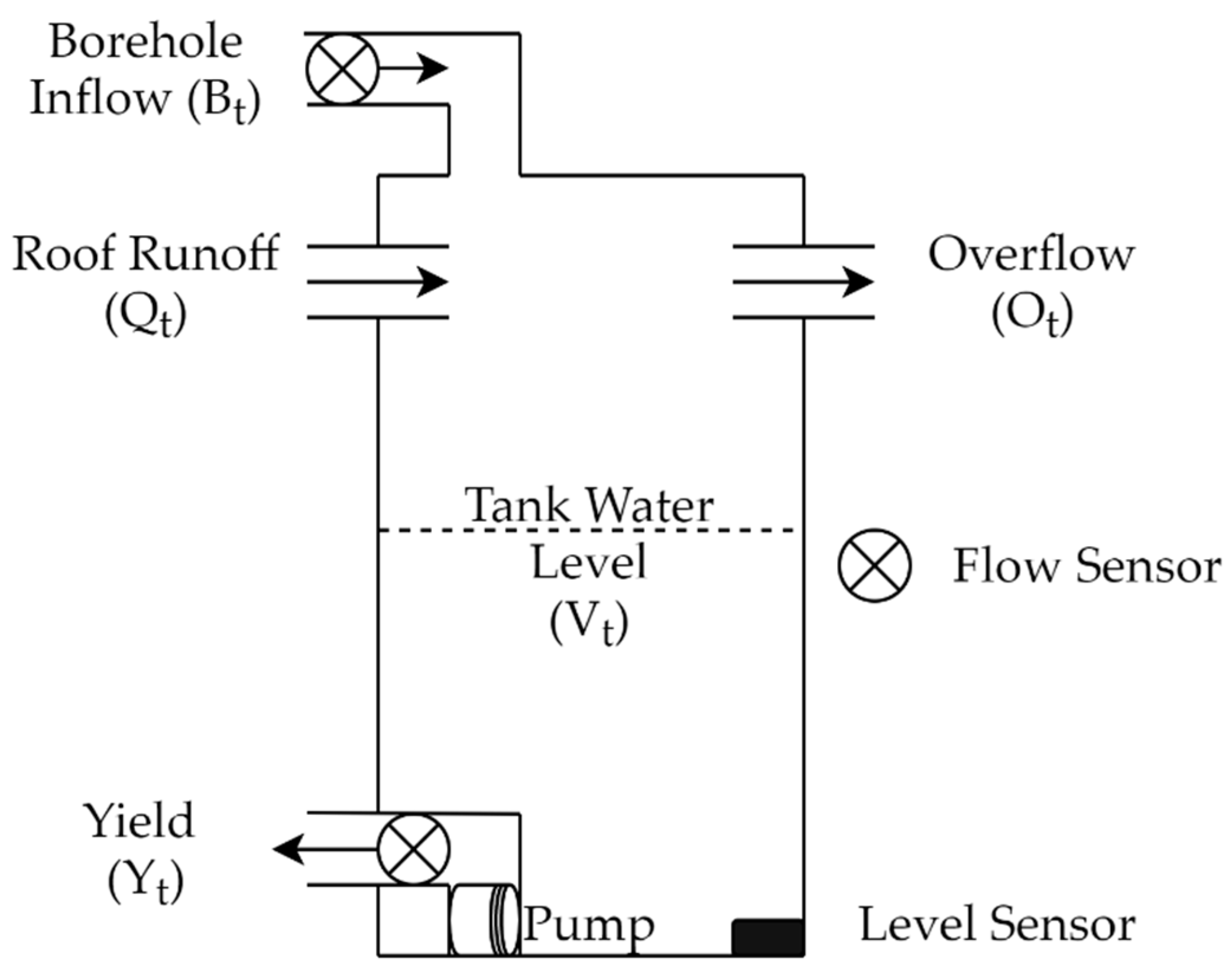
The inflows, outflows and tank levels of three household RWH tanks were monitored. The tanks were connected to a single toilet and, in one case, additionally a washing machine. These houses are part of a unique community located in Broadhempston, Devon, United Kingdom, and are partially owned by the Broadhempston Community Land Trust, which is a Community Interest Company that was set up in 2012 to enable local people, in housing need, to develop affordable eco-housing. This development is not connected to a centralised water supply system and the six families rely on a private borehole to meet their needs. At times, this has proven insufficient. The development’s borehole was upgraded in early 2018 with an additional storage tank added. Technical and financial barriers prevented further upgrades being undertaken and the community continues to experience interrupted water supply. This, in addition to the eco-friendly aspirations of the local community, made the retro-fitting of RWH tanks an attractive option to the householders.

Each property was broadly of the same design and identical RWH tanks (0.8 m³) were installed at the rear of each house in May 2018. Two outflows were possible: spillage through an overflow downpipe located at the top of the tank (not measured) and yield to the toilet delivered by a submersible pump (measured with a flow meter). Two possible inflows were also present: roof runoff (not measured) and additionally residents could choose to top up the water in the tank using the borehole (measured with flow meter). The tank level was continuously measured using a pressure sensor. All sensors were connected to a datalogger and data was recorded at one-minute intervals. The systems were installed by technicians from a telemetry provider and were checked periodically throughout the monitoring period. In addition, the systems were not managed and were emptied solely by the householder for their non-potable water demand. Remote access to the systems was limited, as it was reliant upon consistent availability of householder Wi-Fi. The monitoring period was between 10 June 2018 and 28 August 2019. A schematic of this system is shown in Figure 1.

As water falling below the pump’s inlet could not be supplied to the household, the tanks were found to have an effective tank storage capacity of 0.67 m³. All houses had identical 6/4 L dual-flush toilets and each house had an occupancy rate of two adults and three children. Each roof feeding the downpipes had a plan area (A) of 41.5 m² and the closest rain gauge (Environment Agency 46103) was located 6.5 km from the site at Buckfast.

Drainage on site is provided by a traditional pipe network that feeds a series of swales and other sustainable drainage systems.

2.2. Model Creation and Validation

Each system was modelled using a yield-after-spillage approach (This model is available in supplementary material S1), which is the most conservative method of simulating RWH system behaviour [18]:

$${\mathrm{O}}_{\mathrm{t}}=\max \{\begin{array}{c}0\\ {\mathrm{V}}_{\mathrm{t}-1}{+\mathrm{B}}_{\mathrm{t}}{+\mathrm{Q}}_{\mathrm{t}}-\mathrm{S}\end{array}$$

(1)

$${\mathrm{Y}}_{\mathrm{t}}=\min \{\begin{array}{c}{\mathrm{D}}_{\mathrm{t}}\\ {\mathrm{V}}_{\mathrm{t}-1}\end{array}$$

(2)

$${\mathrm{V}}_{\mathrm{t}}=\min \{\begin{array}{c}{\mathrm{V}}_{\mathrm{t}-1}{+\mathrm{Q}}_{\mathrm{t}}{+\mathrm{B}}_{\mathrm{t}}{-\mathrm{Y}}_{\mathrm{t}}\\ {\mathrm{S}-\mathrm{Y}}_{\mathrm{t}}\end{array}$$

(3)

where O_t is the tank overflow, B_t is the borehole inflow, Q_t is the roof runoff, Y_t is the yield and D_t is the demand during the current time interval t, V_t and V_t−₁ are the volume in store at time step t (current) and t−1 (previous) and S is the tank storage capacity. These all have units of m³ and a 5 min time step. The roof runoff was calculated using:

$${\mathrm{Q}}_{\mathrm{t}}{=\mathrm{R}}_{\mathrm{t}}\mathrm{A}$$

(4)

where R_t is the rainfall at time t (m/5 min); losses were assumed to be zero.

The tank level and recorded inflows and outflows were measured at 1 min resolution, enabling individual toilet usage events to be captured in the data. However, as the rainfall data was only available at hourly intervals, a 1 h time step was necessary for model validation. Although an hourly or coarser time step has previously been used to model the water management potential of stormwater management devices, it has been suggested that a shorter resolution is needed to accurately measure detention performance [15]. In this case, a higher resolution rainfall dataset was unavailable for the monitored data. However, a 5 min interval was used for the long-term simulation, which is detailed in Section 2.4.

The accuracy of the model was assessed using the root mean square error (RMSE) and the coefficient of determination (R²). Each of these indexes gives different model evaluations. By utilizing both, an overall picture of its accuracy can be gathered.

Data from the pressure transducer was used to infer a water demand profile for each house. A uniform demand profile was generated and used in the modelled simulations. This enabled the model to be run based on a site-specific value for daily water demand, and it is acknowledged that such a value would not be available at the design stage. This was performed to examine the impact on accuracy of assuming constant demand, as a time series-based demand profile is not always available.

2.3. Assessment Metrics

The metrics chosen for performance analysis evaluated both objectives of the RWH system: water supply and stormwater management. Relevant metrics were taken from Xu et al. [11] and represented both volumetric (efficiency) and frequency characteristics. The water supply metrics were as follows:

$${\mathrm{E}}_{\mathrm{WS}}=\frac{{{\displaystyle \sum }}^{}{\mathrm{Y}}_{\mathrm{t}}}{{{\displaystyle \sum }}^{}{\mathrm{D}}_{\mathrm{t}}}$$

(5)

$${\mathrm{N}}_{\mathrm{t}}=\{\begin{array}{c}{1,\mathrm{Y}}_{\mathrm{t}}\ge {\mathrm{D}}_{\mathrm{t}}\\ 0,\mathrm{else}\end{array}$$

(6)

$${\mathrm{F}}_{\mathrm{WS}}=\frac{{{\displaystyle \sum }}^{}{\mathrm{N}}_{\mathrm{t}}}{\mathrm{n}}$$

(7)

where E_WS is the water supply efficiency, N_t is counted if demand is satisfied in timestep t, n is the total number of timesteps and F_ws is the water supply frequency. The stormwater management metrics were as follows:

$${\mathrm{E}}_{\mathrm{R}}=\left[1-\frac{{{\displaystyle \sum }}^{}{\mathrm{O}}_{\mathrm{t}}}{{{\displaystyle \sum }}^{}{\mathrm{Q}}_{\mathrm{t}}}\right]$$

(8)

$${\mathrm{N}}_{\mathrm{to}}=\{\begin{array}{c}1, {\mathrm{O}}_{\mathrm{t}}\ge 0\\ 0,\mathrm{else}\end{array}$$

(9)

$${\mathrm{F}}_{\mathrm{o}}=\frac{{{\displaystyle \sum }}^{}{\mathrm{N}}_{\mathrm{t}}}{\mathrm{n}}$$

(10)

where E_R is stormwater retention, N_to is counted if overflow occurs at timestep t and F_o is overflow frequency.

In addition, as the site drainage is limited to swales and other forms of sustainable drainage, the retention below greenfield runoff (E_GF) and the frequency above it (F_GF) are also reported. It is important to limit the inflow into these sustainable drainage features to as low a rate as possible to preserve channel morphology, limit scour and, overall, maintain their utility. The greenfield runoff rate modelled was assumed to be 2 L/s/ha in line with guidance issued on sustainable drainage systems [16].

2.4. Long-Term Modelling and Assesment

In order to investigate the long-term impact of the different household demand behaviours, rainfall inputs for the model were taken from the UK Climate Projections for Cornwall, as detailed in Stovin et al. [15]. This is a 30 year dataset that has been disaggregated into 5 min time steps using the STORMPAC disaggregation tool [18,19].

In addition to examining current demand patterns, scenarios intended to improve the stormwater management performance of these systems were also modelled:

• Scenario 1—Increase demand for non-potable water
  Use of the downstairs toilet was increased and all washing machines were connected to the tank. Each of the five occupants was assumed to use the toilet four times per day on weekdays and six times per day on weekends with a partial flush ratio of 1(6 L):2(4 L) [3]. The washing machine was assumed to have 0.2 uses per day per person, with 50 L per use [3]. In total, demand from the RWH tank was assumed to be 156 L per household per day.
• Scenario 2—Model passive system
  The model was configured to enable passive releases from the tanks to occur. These systems have a slow-release discharge outlet and water below this outlet was stored for domestic consumption. The outlet was sized so that the water above it slowly discharged at the greenfield runoff rate (2 L/s/ha). The passive outlet was located at 0.68 m above the base of the tank, which created a storage capacity of 25% of the effective volume (0.17 m³). The objective of this system is to store runoff during events and allow it to slowly release to the environment.
• Scenario 3—Model active system
  Active release systems were modelled. These were remotely controlled in real time, and they managed the release of water according to the rainfall forecast and available retention volume in the tank. The target was to minimize rainfall discharge by maximizing functional tank capacity prior to the forecasted storm event. The system was emptied at midnight as needed. The pre-storm release volume was calculated as the difference between the available tank storage volume at the end of the previous day and predicted runoff volume for the next 24 h. This pre-storm release was delivered through a 10 mm automated valve located at 0.1 m above the outlet to ensure that there was water above the pump at all times. The pre-storm release was driven by gravity. The objective of this system is to release water quickly in advance of an event in order to provide additional storage capacity.

For scenarios 2 and 3, controlled (passive and active) release was assumed to occur before yield, resulting in a modified overflow (O_t) equation:

$${\mathrm{O}}_{\mathrm{t}}=\max \{\begin{array}{c}0\\ {\mathrm{V}}_{\mathrm{t}-1}+ {\mathrm{B}}_{\mathrm{t}}{+\mathrm{Q}}_{\mathrm{t}}+ {\mathrm{C}}_{\mathrm{t}}-\mathrm{S}\end{array}$$

(11)

where C_t is the controlled release at time t and is calculated using the orifice equation [9]:

$${\mathrm{C}}_{\mathrm{t}}=\mathrm{Cd}\left(\frac{1}{4}{\mathsf{\pi }\mathrm{d}}^2\right)\sqrt{{2\mathrm{gh}}_{\mathrm{t}}}$$

(12)

where d is the orifice diameter, h_t is the head acting over the centreline of the orifice, Cd is the orifice discharge coefficient (Cd = 0.7 was adopted), and g is the acceleration due to gravity (9.81 m/s²).

As well as applying the metrics defined above to the 30 year time series, individual storm events were isolated from the continuous simulation record based on an assumed six-hour inter-event period, as reported by Stovin et al. [20]. The 30 largest events (by volume) were chosen for further analysis. They represented the events with a 1 year return period. These events were considered to be important, as their peak runoff rates were likely to be significant for the morphology and ecology of the catchment [16]. They were analysed using both retention proportion and flow duration curves. Flow duration curves were used as they capture the consequences of both controlled flows and spill from the top of the RWH systems. A flow duration curve is a plot of runoff versus the percent of time for which a particular runoff was equalled or exceeded.

3. Results

3.1. Collected Data

A summary of the data collected is shown in

Table 1. Summary of data collected.

Measurement	House A (Demand: Toilet)	House B (Demand: Toilet and Washing Machine)	House C (Demand: Toilet)
Water Level (m)	10 June 2018–28 August 2109 Missing data: 30 July 2018–25 October 2018 7 July 2019–18 July 2019 There was an unexplained jump from 1.62 to 1 m at 8 am on 20 June 2019	12 March 2019–28 August 2019	1 September 2018–28 August 2019 Missing data: 12 October 2018–29 October 2018 15 November 2018–20 November 2018 25 December 2018–30 December 2018 13 January 2019–19 January 2019 17 February 2019–10 March 2019 14 April 2019–01 June 2019 10 June 2019–16 June 2019 23 June 2019–20 July 2019
Borehole Inflow	10 June 2018–5 February 2019 Missing data: 30 July 2018–25 October 2018	None	1 September 2018–28 August 2019 Missing data: Same as above
Yield	10 June 2018–5 February 2019 Missing data: 30 July 2018–25 October 2018	None	1 September 2018–28 August 2019 Missing data: Same as above

(This data is available in supplementary material S2). It is clear from Table 1 that there were large periods with gaps in the field data. This was due to issues with communication (WiFi), freezing weather, and low maintenance capacity.

Figure 2 shows the recorded water level during the monitoring period for each of the houses. Shaded areas indicate the periods which were chosen for further examination and model validation, as these periods had the most complete dataset. For House A (Figure 2a), this was the period between 26 October 2018 and 4 February 2019. Out of the 102 days examined, the tank was full (water level > 1.8 m) for 46 days and was never empty (water level < 0.2 m). During this period, the average water use from the tank was 46.1 L/day.

For House B (Figure 2b), the period between 12 March 2019 and 13 April 2019 was studied. Out of the 33 days examined, the tank was full for four days (water level > 1.8 m) and empty for 1 day (water level < 0.2 m). However, neither the inflow to the tank from the borehole or outflow to the toilet was measured at this house. It was assumed that no top-up inflow from the borehole occurred, as no inflows equivalent to the pumping rate (8 L/s) were observed. To calculate yield, days were selected where no inflow into the system (no tank level rises) and no rainfall at the weather station was observed. Sixteen of these days were identified and had an average water demand of 48.3 L/day.

For House C (Figure 2c), the period between 11 March 2019 and 13 April 2019 was chosen for further examination. Out of the 34 days examined, the tank was full for 9 days (water level > 1.8 m) and never empty (water level < 0.2 m). During this period, the average water use was 26.5 L/day.

3.2. Model Validation and Short-Term Performace Assesment

Validation of the yield-after-spillage model for each house is shown in Figure 3. Two demand patterns were applied—the first used demand recorded by the flow meter and the second used a constant hourly demand based on the average daily use derived in Section 3.1. The efficiency indexes for the comparisons between the model and measured data are shown in

Table 2. Efficiency indexes for model validation.

House	Root Mean Square Error (RMSE) (m)		Coefficient of Determination (R2)
	Measured	Constant	Measured	Constant
House A (Daily Demand = 46.1 L)	0.25	0.24	0.78	0.8
House B (Daily Demand = 48.3 L)	-	0.12	-	0.95
House C (Daily Demand = 26.5 L)	0.2	0.12	0.97	0.94

.

For House A (Figure 3a), the model replicated the recorded data accurately until 18 January 2019, when the model predicted a significantly higher tank level (maximum of 139% higher). This was attributed to discrepancies between the rainfall used as a model input (from a rain gauge located 6.5 km away from site) and rainfall on site or potentially blocked guttering. For House B (Figure 3b), as demand was not monitored, only constant demand was modelled, and the results agreed well with the monitored water level. For House C (Figure 3c), between 24 March 2019 and 4 April 2019, there was a sizable difference between the model and monitored data, once again attributed to non-localized rainfall data. In all cases, the model represents the monitored data well (R² > 0.78), with no substantial difference between the demand patterns.

The short-term water supply and stormwater management performance calculated using the constant demand pattern is shown in

Table 3. Short-term water supply and stormwater management performance.

Performance Metric	House A 26 October 2019–04 February 2019	House B 12 March 2019–13 April 2019	House C 11 March 2019–13 April 2019
Water Supply Efficiency (Ews) (-)	>0.99	>0.99	>0.99
Water Supply Frequency (Fws) (-)	>0.99	>0.99	>0.99
Overflow Frequency (Fo) (-)	0.17	0.06	0.07
Retention (ER) (-)	0.13	0.41	0.23
Frequency Above Greenfield Runoff (FGF) (-)	0.15	0.05	0.06
Retention Below Greenfield Runoff (EGF) (-)	0.14	0.41	0.23

. It is clear that, as these systems were optimised for water supply, their performance as rainwater management devices was highly dependent upon household use. This is particularly evident in the comparison between House B (12 March 2019–13 April 2019) and House C (11 March 2019–13 April 2019), where there was a 22% difference in runoff reduction purely owing to the lower demand of House C. It is also evident that the retention varies depending on the time period monitored, with House A having significantly less retention during its validation period (26 October 2019–4 February 2019) than House B (11 March 2019–13 April 2019) despite similar water demands.

As the demand was constant, the water supply efficiency and frequency were analogous. In addition, in all cases, the supply met the demand over 99% of the time, indicating that the tanks were correctly sized for water supply. The total retention and retention below greenfield runoff were similar.

3.3. Long-Term Modelling

Table 4. Long-term water supply and stormwater management performance for current demand.

Performance Metric	House A	House B	House C
Ews (-)	0.98	0.98	0.99
Fws (-)	0.98	0.98	0.99
Fo (-)	0.06	0.06	0.07
ER (-)	0.29	0.30	0.18
FGF (-)	0.03	0.03	0.04
EGF (-)	0.34	0.35	0.23

shows the performance results for the 30 year long-term modelling simulation. Similar to the short-term validation study, the water supply frequency and efficiency were equivalent. This is due to the constant demand profile. Although, the houses with larger demand (Houses A and B) retained more water than House C, this retention was still relatively low (max 0.3).

As detailed in Section 2.4, three scenarios were proposed to improve stormwater management through either increasing demand or physically augmenting the tank. The results are shown in

Table 5. Long-term average water supply and stormwater management performance for suggested modelled scenarios.

Performance Metric	Conventional (Conv)	Passive (Pass)		Active (Act)
	Maximum Demand	House B	House C	House B	House C
Ews (-)	0.65	0.78	0.91	0.96	0.99
Fws (-)	0.65	0.78	0.91	0.96	0.99
Fo (-)	0.02	0.29	0.34	0.01	0.01
ER (-)	0.66	0.24	0.16	0.30	0.17
FGF (-)	0.01	0.005	0.005	0.01	0.01
EGF (-)	0.67	0.87	0.86	0.30	0.18

. Only Houses B and C are displayed for the passive and active systems, as they represented the highest and lowest demands respectively. For the maximum demand scenario, the water supply efficiency decreased as the demand increased, which meant that only 65% of household demand could be obtained from the RWH system. Nonetheless, this resulted in a retention efficiency higher than the other scenarios examined. For the passive system, although between 86% and 87% of the system overflow had been reduced to below greenfield runoff, the overall retention was decreased to a level lower than the original systems (Table 4). The active scenario had almost identical retention to the original systems. However, the frequency of overflow decreased. This decrease was caused by the high flow rate of controlled pre-storm release, which results in a similar volume of water release but in a shorter time scale, and this additionally caused a drop in retention below greenfield runoff.

Although Table 5 gives an overall indication of the system performance, the information is insufficient for drainage designers who are typically interested in performance during rainfall events with a 1 year return period or greater.

The 30 Largest Events by Cumulative Volume

Figure 4 shows the retention and flow duration curve of the different systems for the 30 largest events. For the original demand (Figure 4a), retention during these 30 events was significantly worse than the average values observed in Table 5, with mean values between 0.04 and 0.07. However, House B, which has the highest water demand, still performs the best, with an average value of 0.07. For the suggested improvements (Figure 4b), the maximum demand scenario performed the most favourably, whereas the passive systems exhibited the worst retention. Conversely, when the retention below greenfield runoff is examined, both passive systems perform significantly better than the maximum demand scenario, which in turn still outperforms the active systems. In addition, when the flow duration curves are examined for both House B (Figure 4e) and C (Figure 4f), the active system causes an increase in flow rate above roof runoff due to the release being solely controlled by gravity.

4. Discussion

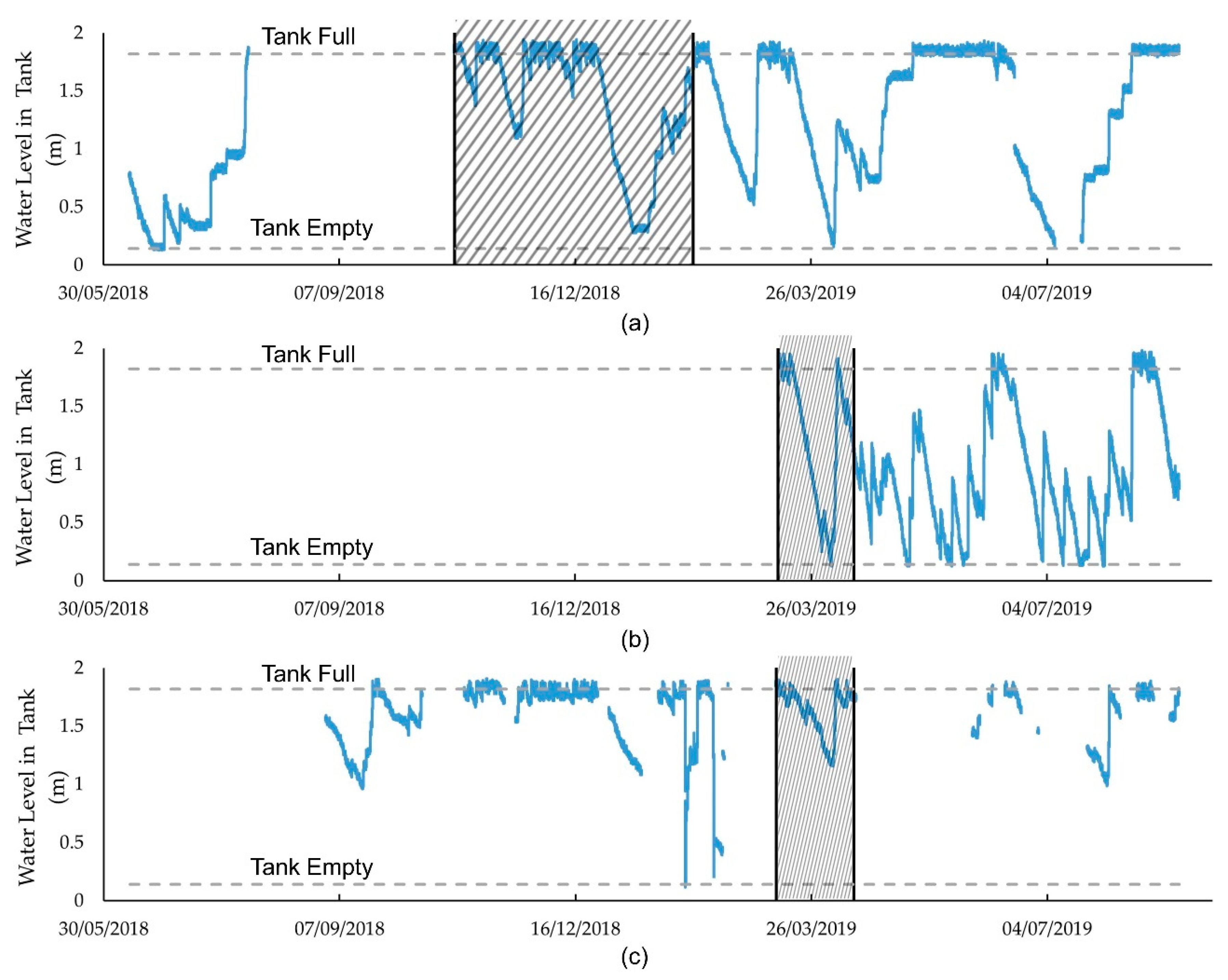
In contrast to previous modelling studies, in which all houses were assumed to have the same demand [9], the findings from Broadhempston showed that households with similar demographics can have substantially different usage rates. In addition, the tanks remained full for between 12% and 45% of the observed validation period, indicating that available water was not being used by the households. This would have an impact on stormwater management, as a full tank offers no stormwater storage potential. These findings indicated that there was potential to further raise the demand from these systems by engaging with the community to increase the usage of the downstairs toilet or connect additional washing machines.

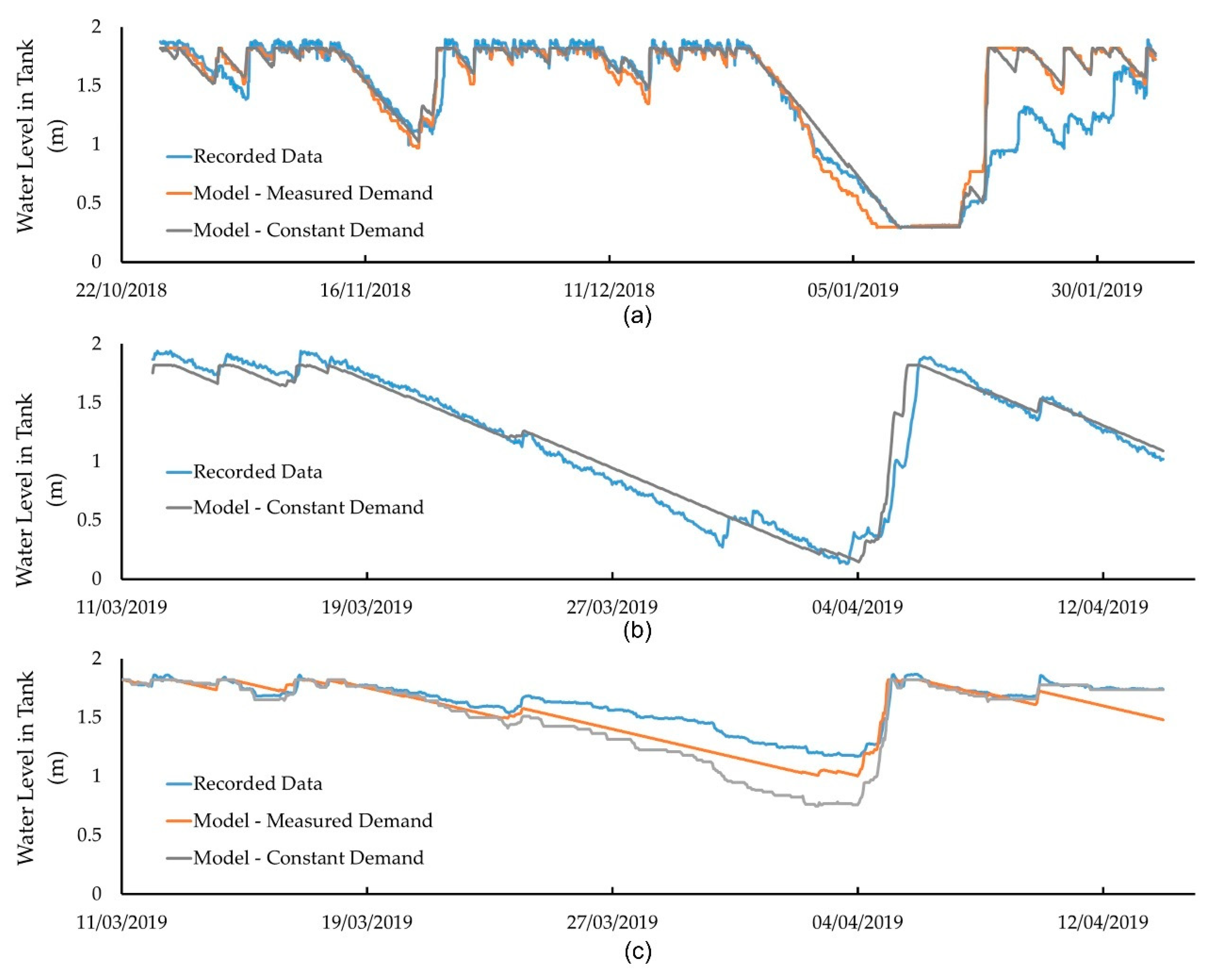
From the model validation study, no significant decrease in accuracy was shown when an average constant demand profile was used as opposed to a metered demand time series. This indicates that a constant demand pattern provides an alternative method of representing demand in a yield-after-spillage model if higher resolution data is unavailable. This is useful in scenarios for which water requirements are not consistently monitored. For a constant demand profile, the water supply frequency and efficiency metrics were equivalent, suggesting that only one of these metrics needs calculation when using this method.

It was found that the greatest source of inaccuracy during model validation was the non-localised rainfall data. This is problematic for models which predict the performance of these systems before they are installed, as data may not be available at the site level. This also raises questions for the emptying accuracy of active systems, as they rely on weather forecasts which may have a high degree of variability depending on local conditions and topography. It is noted that the study also implemented a “perfect forecast” approach, and the accuracy of site-specific forecasts represents a topic for further exploration before such methods can be demonstrably useful.

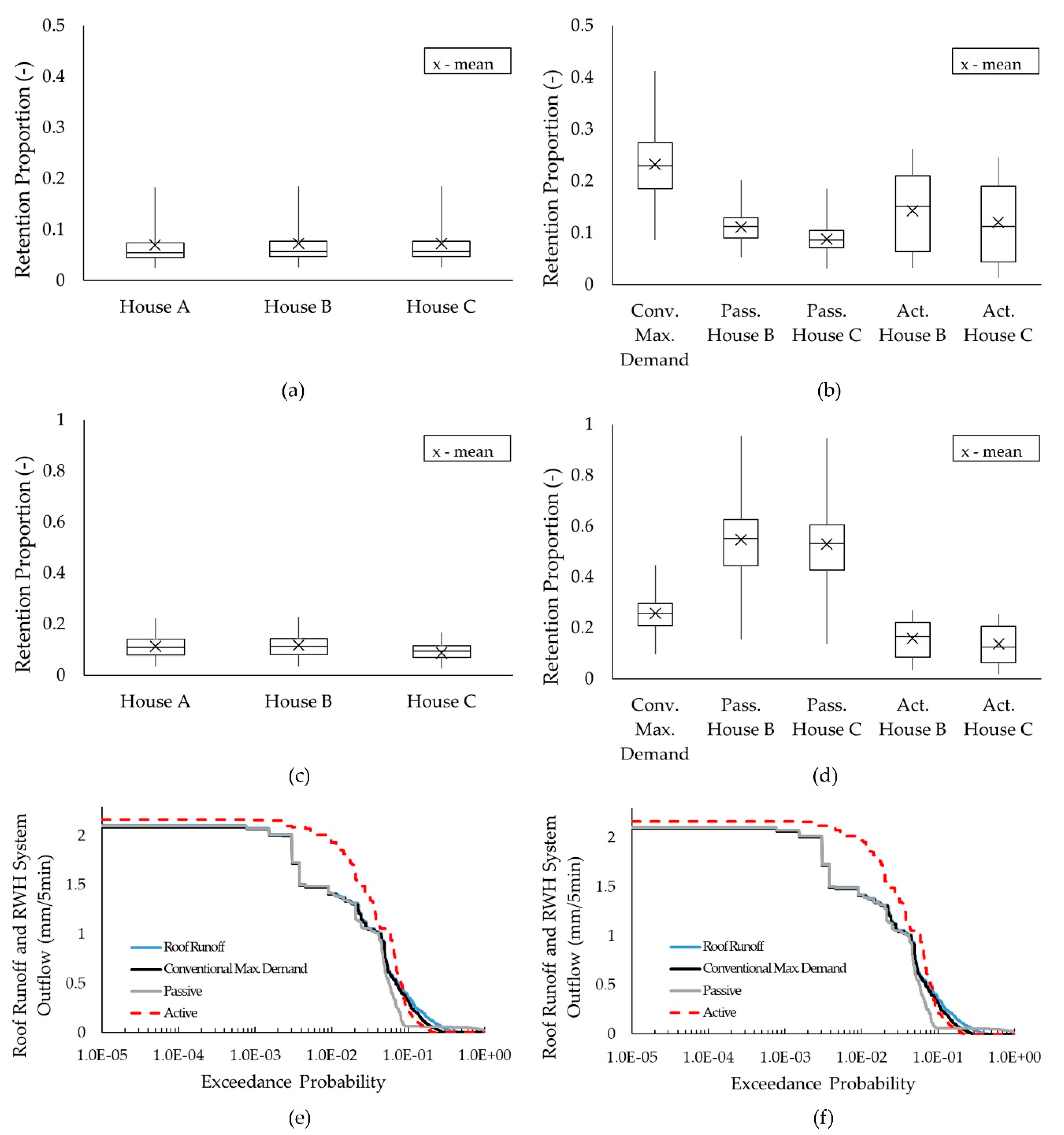
As shown by the periods of downtime in the monitoring data (Figure 1), obtaining a complete dataset of results proved difficult. This was due to intermittent communications which relied upon householder WiFi connections. Without a steady stream of communication from the telemetry, sensor failures could not be identified, or rectified, in a timely manner. These communication challenges will need to be overcome for the successful implementation of active systems and further work is warranted to explore the benefits of a range of communication protocols that could support active technologies to be reliably adopted. For both short- and long-term simulations, as the original systems were designed with the objective of water supply, their functionality was solely dependent on demand. This results in the house with the highest demand (House B) having higher stormwater retention than the house with the lowest demand (House C). For the long-term simulation, although the tanks were designed for water supply, they still exhibited a degree of stormwater management capacity with retention efficiencies of between 0.18 and 0.30. However, overall retention was not a clear indicator of performance, as typically system response to rainfall events with return periods of 1 year or greater is of importance to drainage designers. These events have the capacity to impact surface water quality, disrupt the natural morphology of the catchment or, in extreme cases, initiate flooding. When the retention during the 30 largest events (1 year return period) was examined, it was found that the modelled systems offered little protection, with a mean modelled retention performance of between 0.04 and 0.07. This suggested that, for the demand levels recorded during this study, additional action would be needed to improve stormwater management performance if these systems were to provide adequate runoff control for extreme storm events.

Three scenarios which could improve stormwater management were examined: raising demand and installing passive and active systems. Active systems have been found to be generally superior in simultaneously achieving water supply and stormwater retention compared with the other types of system tested, though it was acknowledged that the control algorithm needs to be implemented carefully [9]. However, this study found that the highest overall retention was exhibited by the maximum demand scenario. In addition, the passive systems have a low overall retention and high overflow frequency rate. Nonetheless, if the frequency and retention of greenfield runoff is examined, it is clear that these systems successfully restricted a minimum of 86% of overflow to below greenfield runoff throughout the 30 year simulation period. Although the active release system limited the amount of time overflow occurred, it did not effectively limit overflow to greenfield runoff, which is indicated by the minimal difference between overall retention and retention below greenfield runoff. This was due to the modelled active pre-release outlet having a diameter designed to deliver high flow rates in advance of a storm. It is noted that this outlet could also be sized to deliver a greenfield runoff rate, though there is a trade-off, as this would impair its ability to empty quickly.

The overflow rates were examined in greater detail during the 30 largest case events through the creation of flow duration curves. They showed that the modelled active system caused a substantial increase in outflow rate above roof runoff. This could have unintended consequences such as eroding the banks of the swales or damaging the morphology of the other on-site sustainable drainage systems. The advantage of active systems is their ability to minimize periods of overflow (shown here through low overflow frequency) and restrict it to outside of rainfall events, which limits the burden of conventional sewers. In addition, these systems did not provide higher retention (mean values of 0.12 and 0.14) than simply increasing demand (0.24). This illustrates that engaging with the community and maximising their demand from the system can yield greater benefits than engineering solutions alone. However, if limiting to greenfield runoff is a principle objective, then passive systems perform best. Although this paper has shown that RWH systems principally designed to provide water supply can effectively work as stormwater management devices, further work is needed to determine the best methods of increasing the performance of the tanks with low demand. This may take the form of community engagement activities or conversion to passive devices if limiting overflow to greenfield runoff is deemed to be sufficient. In addition, as illustrated above, the conventionally used stormwater metrics which represent overall average performance are insufficient at providing guidance relating to system behaviour during individual rainfall events. Further research is needed into the development of more robust metrics which could be used by drainage designers who wished to incorporate these devices in their plans. Further work on the application of active control systems in rainwater and stormwater management is also warranted. Such studies are necessary to explore design philosophies, benchmark their performance and gather empirical data on their performance at pilot sites.

5. Conclusions

In this paper, the current, future and potential water supply and stormwater management performance of domestic RWH systems was evaluated though interrogation of empirical data and modelled scenarios. The conclusions include:

• The short-term monitoring of RWH systems showed large differences in demand between identically sized households. In addition, all tanks were full for long periods, showing that the homes often had spare rainwater available for use.
• Uniform demand profiles, as opposed to a high-resolution time series of metered demand, did not significantly affect the accuracy of a yield-after-spillage RWH system model.
• The retention (E_R) of the systems over a thirty year period was modelled to be between 0.17 and 0.30 depending on demand. However, this decreased to between 0.04 and 0.07 when the 30 largest events were examined.
• Modelling indicated that increasing demand from the system increases overall retention to a greater degree than converting them to passive or active systems. This illustrates the value of engaging the community and that, through maximizing their demand for the available non-potable water, greater benefits can be achieved than through engineering solutions alone.
• During the long-term modelling simulation, passive systems were the most effective at reducing overflow to below greenfield runoff, whereas active systems substantially increased flow rates above roof runoff during the 30 largest events.