Rainstorm Magnitude Likely Regulates Event Water Fraction and Its Transit Time in Mesoscale Mountainous Catchments: Implication for Modelling Parameterization

Abstract

Event water transit time estimation has rarely been done for violent rainstorms (e.g., typhoons) in steep and fractured mountainous catchments where the range of transit time, potential controlling factors, and the validity of time-invariant parametrization are unclear. Characterized by steep landscape and torrential typhoon rainfall, Taiwan provides great opportunities for inquiring into the above questions. In this study, the hydrometrics and δ¹⁸O in rainwater and streamwater were sampled with a ~3-h interval for six typhoon events in two mesoscale catchments. The TRANSEP (transfer function hydrograph separation) model and global sensitivity analysis were applied for estimating mean transit time (MTT_ew) and fraction (F_ew) of event water and identifying the chronosequent parameter sensitivity. Results showed that the MTT_ew and F_ew varied from 2.0 to 11.0 h and from 0.2 to 0.8, respectively. Our MTT_ew in the mesoscale catchments is comparable with that in microscale catchments, showing a fast rainfall-runoff transfer in our steep catchments. The average rainfall intensity is a predominant indicator, which negatively affects the MTT_ew and positively affects the F_ew, likely activating preferential flow-paths and quickly transferring event water to the stream. Sensitivity analysis among inter- and intra-events demonstrates that parameter sensitivity is event-dependent and time-variant. A quick and massive subsurface flow without distinct mixing with groundwater would be triggered during large rainstorms, suggesting that time-variant parameterization should be particularly considered when estimating the MTT_ew in steep and fractured catchments at rainstorm scale.

1. Introduction

Transit time chronicling the elapsed time of water from entering a system, traveling through the system to its exit [1], is a single integrated measure at the outlet, which is affected by sources, pathways, and water storage, and thus is indicative of how catchments retain and release water and solutes associated with biogeochemical processes [2], chemical weathering [3], and contamination transport [4,5]. Therefore, accurately estimating characteristics of transit time distribution (TTD, e.g., means, medians, and shape parameters of distributions) is an informative way to understand hydrological behaviors, biogeochemical effects [6], and land-cover changes [7,8]. Typically, TTDs are mainly derived from an assumed functional form (e.g., exponential or gamma distribution) whose time-variant and time-invariant parameters are estimated from passive tracers and hydrological data [9,10]. While the time-variant parameterization with different methodologies is still under development (e.g., [10,11]), the time-invariant parameterization has been applied across many regions since 1990. The accumulated information through time-invariant parameterization has been ample, and a compilation of this information is available for shedding some light in this field of study. For example, Jasechko et al. [12] compiled δ¹⁸O data of rainwater and streamwater from 254 watersheds around the world and applied the sine-wave method (time-invariant assumption) to estimate mean transit time of the catchments. They concluded that young streamflow is less prevalent in steeper landscapes due to long flow-paths and high permeability due to fractured rocks. The new-found territory shows the necessity of further understanding mean transit time (MTT_ew) and fraction (F_ew) of event water during rainstorms.

Previous studies about MTT of total streamflow demonstrated that the topography (e.g., flow-path length and flow-path gradient), bedrock permeability, and connectivity between hillslope and stream rather than the catchment area are the predominant controls on MTT of total streamflow [13,14,15]. However, the dynamics of event water transit time during a rainstorm is rarely studied, not to mention the relationship between MTT_ew and landscape or rainfall forcing. Weiler et al. [16] proposed the TRANSEP (transfer function hydrograph separation) model, which integrates the unit hydrograph and the isotope hydrograph separation (IHS) techniques with the time-invariant assumption to estimate the transit time at event scale. Simply, this model can partition the temporal variability of streamflow into event and pre-event components and thus estimate MTT_ew and F_ew in a quantitative approach. The simplicity and applicability of the model helped in the investigation of 64 catchment-events (17 catchments) around the world (most of them in the temperate zone). Among those studies, the total precipitation of an event was between 2.4 to 177 mm and the catchment area mostly ranged from 0.02 to 8.8 km². Since the responses of rainfall-runoff transfer among rainstorms are diverse and controlled by both static landscape structure and antecedent condition, identifying the influences of landscape and rainfall forcing on MTT_ew, F_ew, and event water TTD-associated parameters needs help from the MTT_ew-associated compilation. For example, McGuire and McDonnell [17] demonstrated that hillslope discharge was a threshold-like response when antecedent rainfall in Oregon was greater than 20 mm. Besides, the rainfall-runoff transfer during a rainstorm is highly temporally variable and thus hypothesized. Two approaches can be taken for evaluating temporally variable parameterization. One approach is to utilize the presumed time-variant parameterization in the model to test the hypothesis [10,18], with an alternative approach to diagnose the temporal sensitivity analysis of time-invariant parameters [19]. Thus, the key parameters regulating event water TTDs during a rainstorm were identified. This provides a potential linkage between key parameters and rainfall forcing.

In this study, rainwater and streamwater of six typhoons during 2012–2015 were collected with a 3-h interval sampling scheme in two adjacent steep mesoscale catchments in subtropical northern Taiwan. The TRANSEP model with gamma distribution as event water TTD was applied to estimate the MTT_ew and F_ew for individual events. Meanwhile, a temporal sensitivity analysis was also applied to determine the variation of parameter sensitiveness during a rainstorm. Specifically, this study aims to investigate: (1) the control of hydrometric input (rainstorm) on MTT_ew and F_ew in steep catchments and (2) the variability of event water TTD-associated parameter sensitiveness during a rainstorm. This study on the event water MTT of extreme rainstorms in mesoscale mountainous catchments, as provided here, may shed new light on MTT model development in the future.

2. Materials and Methods

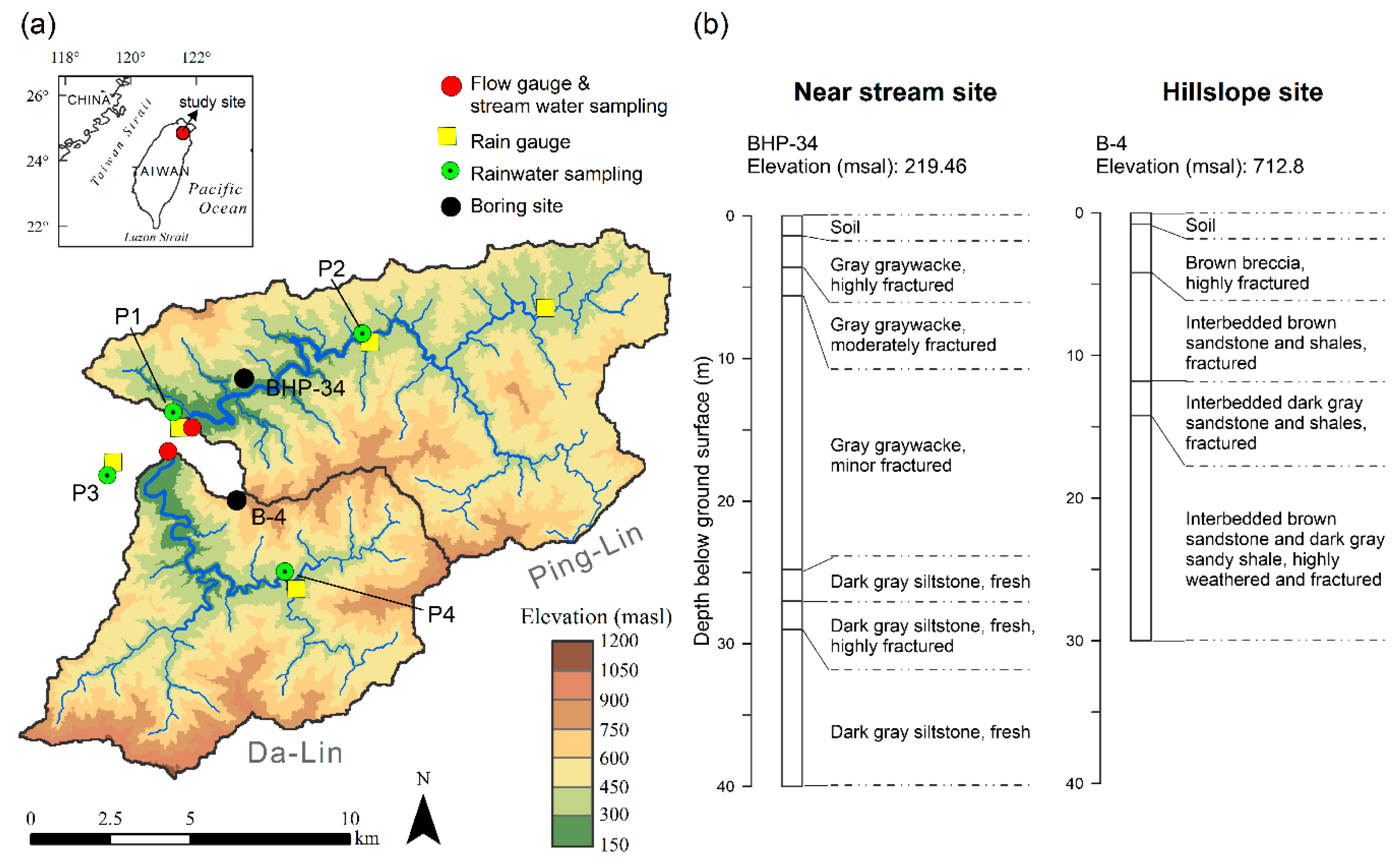
2.1. Study Site

Our study sites, Ping-Lin (PL, 111 km²) and Da-Lin (DL, 79 km²), are two mesoscale mountainous catchments located in northern Taiwan. The elevation ranges from 182 to 994 m, and the mean slope varies from 26° and 30° (Figure 1a). Interbedded sandstone and shale rock uplifted by the collision of the Eurasian plate and the Philippine Sea plate shapes the steep and fractured landscape [20]. Boring logs show that the lithological formations are highly fractured from ridges to streams (Figure 1b, provided by Taiwan Central Geological Survey). Inceptisols with depth less than 1.0 m cover most of the steep hillslopes, while entisols that have high permeability with soil depth around 1.5 m lie mostly in the valley bottoms [21]. Evergreen conifer–broadleaf forest accounts for 90% of the catchment area. Anthropogenic disturbance is strictly limited by the Taipei Water Management Office since the catchments are located within the Taipei Water Source Domain, where the Feitsui Reservoir is the main domestic water supply for the entire Taipei metropolis.

The two catchments are characterized by a subtropical monsoon climate with a mean annual temperature of 20 °C (13 °C in January and 26 °C in July) and precipitation of approximately 4000 mm yr⁻¹. There is no significant seasonality in precipitation but there are, however, different precipitation types. In summer (July–September), precipitation falls mainly with high intensity in the form of a typhoon (approximately 64% of daily rainfall exceeds 10 mm), whereas the precipitation in winter, brought by the East Asian monsoon features long duration and low intensity [21,22]. Echoing the abundant precipitation, the annual runoff is approximately 3400 mm, and the annual potential evapotranspiration is approximately 1000 mm.

2.2. Hydrometrics and Water Isotope Measurement

2.2.1. Hydrometrics

In the study area, there were five rain gauges maintained by the Taiwan Central Weather Bureau (CWB) and the Water Resources Agency (WRA) and two streamflow gauges maintained by WRA providing hourly data (Figure 1). The hourly precipitation data were interpolated using the inverse distance weighting method (exponent coefficient = 2.0) to represent the rainfall heterogeneity (in Supplementary Material). From 2012 to 2015, eight typhoons were sampled and the basic information was collected, including the total precipitation amount (P), duration (D), average intensity of rainfall (RI_avg), maximum 3-h rainfall amount (P_max3h), total runoff (Q), peak flow (Q_max), runoff ratio (Q/P), and the antecedent 7-day rainfall (AP_7day). In the literature, these are considered to be factors affecting event water transit time and event water fraction [23,24,25].

2.2.2. Water Isotope Measurement

Two streamwater sampling sites were set at the same location of streamflow gauges near the catchment outlet. Site PL was at the Ping-Lin Bridge and the other site, DL, at the Da-Lin Bridge (Figure 1). From 2012 to 2015, during every typhoon invasion, water samples were collected at 3-h (storms 1 to 4) to 2-h (storms 5 and 6) intervals. The sampling period lasted from the beginning of rainfall to at least 12 h after the storm. Sampling during typhoon periods in Taiwan takes incredible labor and time, not to mention the danger in the extreme weather. Occasional gaps in the streamwater sampling were due to inaccessibility caused by rock falls or even landslides. Rainwater was also sampled during typhoons. Four rainwater sampling sites were set up within the two catchments, but only the one close to site PL (P1) was sampled with the same frequency as the streamwater while at other sites rainwater of the typhoon was collected as a bulk. The spatial heterogeneity of rainfall and the isotopic composition of rainwater were examined. Typhoon-induced rainfall is short-lived, intense, and its spatial heterogeneity in mesoscale catchments is not considerable, because the strong circulation induced by typhoon becomes a predominant control on precipitation over landscape effect [26]. Our investigation of rainwater isotopic composition, though sparse, also showed an indistinct spatial heterogeneity. Details of the investigation could be referred to in the Supplementary Material (Figure S1 and Table S1).

All water samples were passed through pre-weighed and pre-combusted 0.7-μm glass fiber filters in situ. Filtrates were sealed in centrifuge tubes and stored at 4 °C until analysis back at the lab. δ¹⁸O of all the water samples were measured by PICARRO L2120-i isotopic water analyzer which is a time-based measurement system that uses a laser to quantify spectral features of gas-phase molecules in an optical cavity. Isotope signature was compared to VSMOW in ‰ with the precision of 0.1 ‰.

2.3. Estimation of Mean Transit Time (MTT_ew) and Event Water Fraction (F_ew)

The TRANSEP model, generally used for quantifying the mean transit time and event water fraction [16], was applied onto our catchments. TRANSEP is an event-scale tracer-aided rainfall-runoff model that incorporates the tracer input into an instantaneous unit hydrograph (IUH) so that it can analyze water amount and tracer signal synchronously. The model is briefly described below, and the details and its flow chart could be found in [16].

The TRANSEP model consists of two modules, i.e., the streamflow module and the tracer module. The streamflow module is simply an IUH. First, it estimates the effective rainfall (P_eff) by a loss function that directly contributes to the storm event [27]:

$$P_{eff}\left(t\right)=p\left(t\right)s\left(t\right)$$

(1)

$$\mathrm{s}\left(\mathrm{t}\right)=a_{1}p\left(t\right)+\left(1-a_2{}^{-1}\right)s\left(t-\Delta t\right)$$

(2)

where p(t) and s(t) is gross rainfall amount and wetness condition at t time step, respectively. The s(t) depends on the antecedent rainfall and ranges from 0 to 1. The parameter a₁ constrains the total amount of effective rainfall which equals direct runoff, and a₂ determines the weighting of the rainfall prior to each time step. The antecedent rainfall condition is set as s(0) = a₃. Then, the streamflow at t time step Q(t) is calculated by using a convolution of effective rainfall and runoff transfer function g(τ):

$$\mathrm{Q}\left(t\right)={{\displaystyle \int }}_0^{t}g\left(\tau \right)P_{eff}\left(t-\tau \right)d\tau$$

(3)

The parameters in g(τ) and s(t) could be calibrated by comparing the observed and simulated streamflow.

In the tracer module, the streamflow (Q) is separated into pre-event (Q_p) and event (Q_e) water components, which could be estimated via tracer data as below:

$$Q=Q_p+Q_e$$

(4)

$$CQ=C_p{Q}_p+C_e{Q}_e$$

(5)

where C, C_p, and C_e are tracer (e.g., δ¹⁸O) concentration in streamwater, pre-event water, and event water, respectively. Derived from Equations (4) and (5), the tracer concentration in streamwater can be simulated by the following equation:

$$C\left(t\right)=\frac{Q_e\left(t\right)}{Q\left(t\right)}\left(C_e\left(t\right)-C_p\right)+C_p$$

(6)

This equation assumes no fractionation effect in ¹⁸O from either soil evaporation or canopy interception during storms. Streamflow Q is calculated from Equation (3). Event water component Q_e is estimated by a convolution of event water input and event water transfer function (i.e., TTD_ew). Pre-event water concentration C_p is constant for each event. Note that the time-series amount and isotopic composition of rainwater collected at P1 are used for p and C_e. Specifically, the event water input is estimated through P_eff multiplied by the fraction f, which is defined as the proportion of effective rainfall reaching the stream during the event. The fraction f is estimated by the loss function again; therefore, s, a₁, and a₂ in Equation (2) are replaced by f, b₁, and b₂. Besides, the initial fraction, f(0), is zero as there is no event water at the beginning of the event. The event water component Q_e can, therefore, be estimated by:

$$Q_e\left(\mathrm{t}\right)={{\displaystyle \int }}_0^t{P}_{eff}\left(t-\tau \right)f\left(t-\tau \right)h\left(\tau \right)d\tau$$

(7)

where h(τ) is the event water transfer function representing a time-invariant TTD_ew. After capturing the event water component, the event water concentration C_e could be calculated by the ratio of labeled rainwater tracers to event water runoff:

$$C_e\left(\mathrm{t}\right)=\frac{{{\displaystyle \int }}_0^t{C}_r\left(t-\tau \right)P_{eff}\left(t-\tau \right)f\left(t-\tau \right)h\left(\tau \right)d\tau }{{{\displaystyle \int }}_0^t{P}_{eff}\left(t-\tau \right)f\left(t-\tau \right)h\left(\tau \right)d\tau }$$

(8)

where C_r is the tracer (i.e., δ¹⁸O) concentration in rainwater. Unlike other hydrograph separation and transit time methods, which need a predefined weighting relationship [28], the advantage of this procedure is that it allows direct weighting of the input concentrations.

In the TRANSEP framework, the selection of runoff transfer function and event water transfer function are critical to obtain the MTT_ew and the gamma function (GM) is selected to describe the transfer of water in this study for its flexibility [5,11]. Note that parameters α and β in two transfer functions were illustrated by using footprint (α_q and β_q as for runoff transfer function, and α_e and β_e as for event water transfer function):

$$\mathrm{g}\left(\tau \right)=h\left(\tau \right)=\frac{{\tau }^{\alpha -1}}{{\beta }^{\alpha }\mathsf{\Gamma }\left(\alpha \right)}{e}^{-\frac{\tau }{\beta }}$$

(9)

After optimization of both streamflow and tracer modules, the MTT_ew (= α_e × β_e) and F_ew (= Q_e/Q) could be estimated and the details of the parameter descriptions and their corresponding ranges are listed in

Table 1. TRANSEP model and their uniform sampling ranges for sensitivity analysis and calibration.

Parameter	Description	Range
a1	Weighting the precipitation	0.005–0.1
a2	Exponentially weighting the precipitation backward in time	1–15
a3	Initial antecedent precipitation index	0–1
αq	Shape parameter in runoff transfer function	0.1–3.5
βq	Scale parameter in runoff transfer function	1–100
b1	Weighting the Peff	0–100
b2	Exponentially weighting the Peff backward in time	1–15
αe	Shape parameter in event water transfer function	0.1–3.5
βe	Scale parameter in event water transfer function	1–100

.

2.4. Parameter Calibration

Since the model can simulate both streamflow and tracer, δ¹⁸O in this study, simultaneously, a two-step calibration procedure was suggested [16,29]. In order to constrain the accuracy of the simulated hydrograph, runoff-related parameter sets (a₁, a₂, a₃, and α_q, β_q used in the runoff transfer function,

Table 2. Hydrometric characteristics of the catchment-events. P = total precipitation, D = duration, RI_avg = intensity of rainfall, P_max3h = maximum 3-h rainfall amount, Q = total streamflow, Q_max = peak flow, Q/P = runoff ratio, and AP_7day = antecedent 7-day rainfall.

Catchment Event	Typhoon	Date	P	D	RIavg	Pmax3h	Q	Qmax	Q/P	AP7day
		(year/month/day)	(mm)	(h)	(mm h−1)	(mm)	(mm)	(mm)	(-)	(mm)
PL01	Saola	2012/7/31	699	78	9.0	116	440	20.9	0.63	73
PL02	Soulik	2013/7/12	253	23	11.0	88	120	12.5	0.47	2
PL03	Trami	2013/8/21	319	47	6.8	88	149	11.9	0.47	22
PL04	Matmo	2014/7/22	236	34	6.9	54	135	6.7	0.57	0
PL05	Chan-hom	2015/7/9	261	45	5.8	48	158	6.2	0.61	27
PL06	Soudelor	2015/8/7	414	48	8.6	107	299	22.5	0.72	19
		Average	364	46	8.0	84	217	13.5	0.58	24
DL01	Saola	2012/7/31	934	86	10.9	121	621	27.0	0.66	135
DL02	Soulik	2013/7/12	374	21	17.8	120	196	21.4	0.52	1
DL03	Trami	2013/8/21	345	43	8.0	92	171	13.3	0.50	16
DL04	Matmo	2014/7/22	249	29	8.6	55	178	9.2	0.71	6
DL05	Chan-hom	2015/7/9	247	38	6.5	46	162	6.0	0.66	48
DL06	Soudelor	2015/8/7	612	43	14.2	189	337	34.1	0.55	25
		Average	460	43	11.0	104	278	18.5	0.60	39

) were calibrated via modified Kling–Gupta efficiency coefficient (KGE) [30] as simulation performance. The main advantage of KGE is to consider the correlation (r), variability ratio (V), and bias ratio (B) between simulation and observation within a single performance measure:

$$\mathrm{KGE}=1-\sqrt{{\left(r-1\right)}^2+{\left(V-1\right)}^2+{\left(B-1\right)}^2}$$

(10)

where r is the linear correlation coefficient between the simulated and the observed values, V is a measure of standard deviation ratio of the simulated to the observed values, and B is the ratio between the mean simulated and mean observed, i.e., the bias. In fact, the KGE measures the Euclidean distance from three dimensions, which means that it can optimize correlation, variability, and bias simultaneously. Moreover, KGE_Q values higher than 0.8 was set as the criteria for selecting parameter sets in order to restrict the simulated streamflow for hydrograph separation. Similarly, the tracer-related parameters (b₁, b₂, and α_e, β_e in event water transfer function, Table 1) were calibrated by KGE_C as well. The two KGEs, one for streamflow and the other for the tracer, were simultaneously undertaken to retrieve the representative parameter sets, Pareto front, for each event [31]. The ‘best-performed’ parameter set was retrieved from the highest KGE_C of the Pareto front. In sum, 500,000 random parameter sets were then introduced to the model to get simulations. These simulations were further evaluated by KGE_Q and KGE_C in the Pareto front plot for retrieving the ‘best’ parameter sets.

2.5. Sensitivity Analysis

Sensitivity analysis (SA) is widely used to improve the understanding of model operation and key parameters. This study used EET (elementary effect test), a global SA proposed by Morris [32], to screen out parameters which are negligible on the output variability [33]. Specifically, this method samples parameter sets on grids covering the whole parameter space to identify the sensitiveness of each parameter. This method is a one-at-a-time method, which only perturbs parameter x_i along a grid of size Δ_i without changing other parameters at one time to create a trajectory (parameter set) within the parameter space. The elementary effect (EE) means the output perturbation between the original and the changed input trajectory. The mean of multiple EEs (Morris’s μ_i) is taken as a global sensitivity measure for parameter x_i:

$${\mu }_i=\frac{1}{N}{\displaystyle \sum }_{j=1}^N\left|E{E}_i^j\right|$$

(11)

$$E{E}_i=\frac{f\left(x_1,\dots ,x_i+{\Delta }_i,\dots ,x_M\right)-f\left(x\right)}{{\Delta }_i}$$

(12)

where f(x) represents the function evaluation at the previous point in the trajectory. And the root mean squared error (RMSE) is set to represent the f(x) for incorporating measures of model accuracy [19,33]. For measuring the sensitivity of streamflow and tracer simulation, the RMSE_Q and RMSE_C were computed as the f(x). The sampling size N was set at 20, as Herman et al. [34] did. Because parameters a₁, a₂, and a₃ were constrained by the total amount of effective rainfall and direct runoff, the parameter sensitivity of other six parameters b₁, b₂, α_q, β_q, α_e, β_e was measured for each event and then the key parameters under changing conditions were identified

3. Results

3.1. Hydrometric and Tracer Dynamics among Typhoons

The hydrometrics of the 12 catchment-events are shown in Table 2. Briefly, the mean typhoon rainfall (P) in PL and DL were 364 and 460 mm, respectively, within two days, and ranged from 236 to 934 mm. The average rainfall intensity (RI_avg) of all events varied from 5.8 to17.8 mm h⁻¹, whereas the average maximum 3-h rainfall intensity (P_max3h) was approximately 90 mm with a large variation from 48 to 189 mm among events. The mean total streamflow (Q) in PL and DL was 217 and 278 mm, respectively, which resulted in a runoff ratio (Q/P) of approximately 0.60, and the peak flow (Q_max) ranged from 6.0 to 34.1 mm. The statistics of water isotopic composition of rainwater and streamwater are shown in

Table 3. Statistics of δ¹⁸O isotope composition in rainwater and streamwater used as input data for the modelling.

Catchment Event	Typhoon	Rainwater (‰)					Streamwater (‰)
		n	Average *	SE	Maximum	Minimum	n	Average *	SE	Maximum	Minimum
PL01	Saola	21	−11.6	3.13	−3.4	−15.7	24	−8.6	1.18	−6.3	−10.7
PL02	Soulik	8	−8.5	4.75	2.5	−10.1	13	−7.1	0.99	−4.8	−8.0
PL03	Trami	11	−14.1	4.18	−5.7	−18.1	15	−8.5	0.94	−6.5	−10.0
PL04	Matmo	10	−10.4	3.15	−6.4	−16.0	13	−7.1	1.00	−5.1	−7.8
PL05	Chan-hom	16	−5.3	1.76	−3.2	−8.3	21	−5.6	0.41	−4.8	−6.3
PL06	Soudelor	13	−9.3	4.12	−1.0	−14.1	18	−7.2	1.12	−5.0	−8.5
DL01	Saola	21	−11.2	3.13	−3.4	−15.7	24	−8.8	0.94	−7.0	−11.0
DL02	Soulik	8	−8.0	4.75	2.5	−10.1	12	−6.9	0.60	−5.4	−7.6
DL03	Trami	11	−13.9	4.18	−5.7	−18.1	15	−8.8	0.96	−6.8	−10.3
DL04	Matmo	10	−10.7	3.15	−6.4	−16.0	13	−7.2	0.80	−5.9	−8.3
DL05	Chan-hom	16	−4.8	1.76	−3.2	−8.3	21	−6.8	0.62	−6.1	−8.6
DL06	Soudelor	13	−9.1	4.12	−1.0	−14.1	18	−7.5	0.97	−5.7	−8.7

* Isotope compositions averages weighted by the water amounts.

. Generally, there were over 10 samples for each event, except for event 2 due to its short duration. Regarding inter-event variation, the averaged δ¹⁸O in precipitation of all catchment-events was −8.6‰, with a range of −13.3‰ to −4.9‰, in comparison with −6.9‰ with a range of −8.1‰ to −5.4‰ in streamwater δ¹⁸O. As for intra-event variation, the mean standard deviation (SD) of δ¹⁸O was 2.94 in rainwater and 0.76 in streamwater. In addition, the SE of both rainwater δ¹⁸O and streamwater δ¹⁸O in large events (events 1, 2, and 6) were larger than those in small events (events 3, 4, and 5).

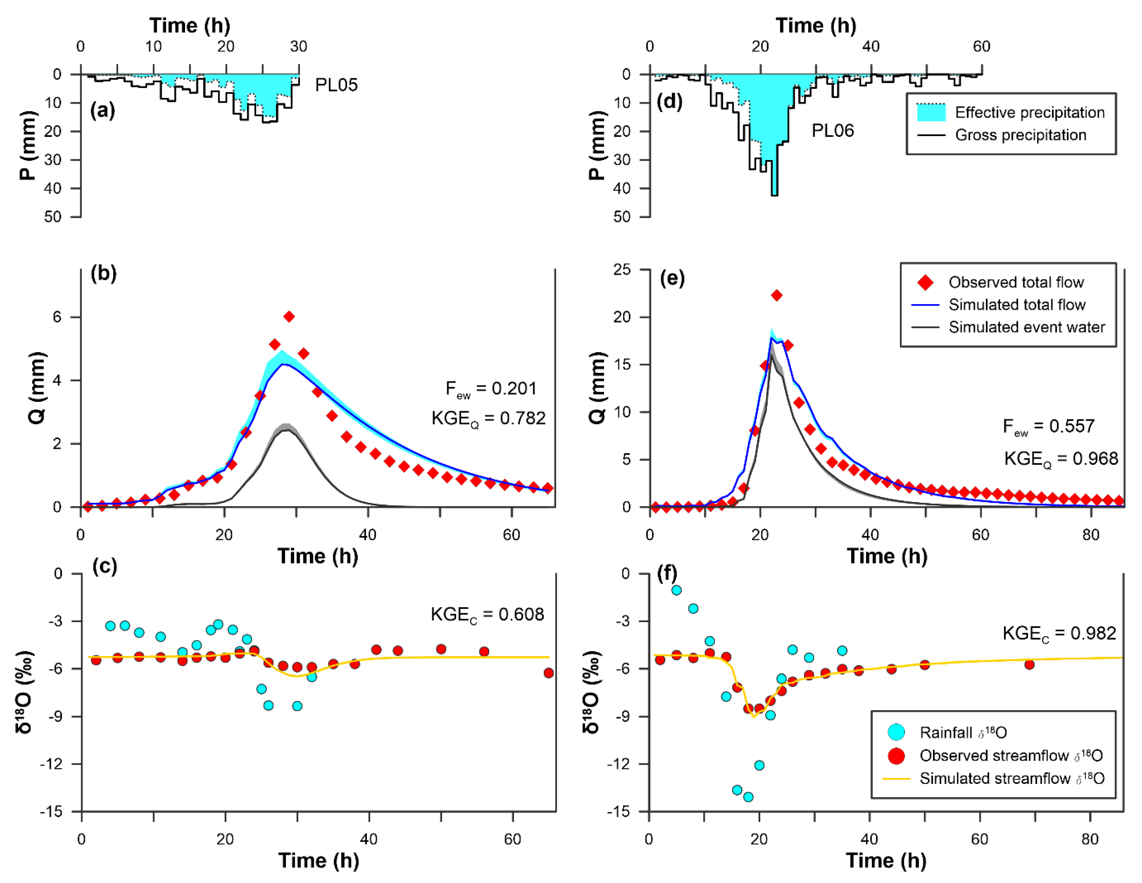
3.2. Simulation Performances and Estimations of MTT_ew and F_ew

The calibrated parameters (α_e, β_e) and the estimated MTT_ew and F_ew are listed in

Table 4. Determined best-performed parameters of event water transfer function and MTT_ew and simulated F_ew.

Catchment Event	αe		βe		Mean Transit Time of Event Water (MTTew)		Fraction of Event water (Few)
PL01	0.68	(0.65–0.80)	8.3	(6.2–8.4)	5.6	(4.9–5.8)	0.33	(0.31–0.33)
PL02	0.80	(0.76–0.80)	5.4	(5.4–5.7)	4.3	(4.3–4.5)	0.39	(0.39–0.40)
PL03	1.45	(1.25–1.46)	2.3	(2.3–2.8)	3.3	(3.3–3.5)	0.14	(0.13–0.14)
PL04	1.90	(1.79–1.94)	3.5	(3.5–4.0)	6.7	(6.7–7.4)	0.41	(0.40–0.42)
PL05	3.01	(2.85–3.21)	1.9	(1.7–2.0)	5.7	(5.5–5.9)	0.20	(0.20–0.21)
PL06	0.78	(0.72–0.79)	7.8	(7.5–8.4)	6.1	(5.5–6.2)	0.56	(0.55–0.57)
DL01	1.10	(0.77–1.19)	4.7	(4.3–7.6)	5.1	(4.9–6.0)	0.24	(0.24–0.29)
DL02	0.56	(0.54–0.62)	4.0	(3.9–4.9)	2.3	(2.3–2.7)	0.59	(0.56–0.59)
DL03	0.72	(0.72–0.81)	12.0	(11.8–13)	8.6	(8.6–10.0)	0.20	(0.17–0.26)
DL04	2.18	(1.72–2.52)	2.5	(1.8–11.2)	5.4	(4.5–22.8)	0.28	(0.28–0.56)
DL05	1.74	(1.63–1.77)	6.3	(5.2–6.3)	10.9	(8.5–11.1)	0.61	(0.56–0.61)
DL06	0.92	(0.88–1.12)	4.2	(3.6–4.4)	3.8	(3.8–4.3)	0.80	(0.79–0.81)

Numbers in parentheses indicate the lower and upper limit among the representative simulations.

. The performance measures, KGE and its element, r, V, and B, are listed in Table S2 of Supplementary Material. In general, both simulations of streamflow and δ¹⁸O were satisfactory for all catchment-events. All KGE_Q for the two catchments were higher than 0.85, and the KGE_C of δ¹⁸O simulation were also satisfactory with ranges of 0.96 to 0.99 and 0.75 to 0.90 in PL and DL, respectively. The details of the individual performance of the three perspectives are referred to Supplementary Material. The parameter α_e varied from 0.68 to 3.01 in PL and from 0.56 to 2.18 in DL. The parameter β_e varied from 1.9 to 8.3 in PL and from 2.5 to 12.0 in DL except for event DL05. The MTT_ew in PL and DL varied from 3.3 to 6.7 h and 2.3 to 10.9 h, respectively. The ranges and variations of the parameters and MTT_ew between the two catchments were similar and consistent. In terms of F_ew, PL and DL varied from 0.14 to 0.56 and 0.2 to 0.8 of the total streamflow, respectively, showing that F_ew in DL were larger than in PL.

The simulations of streamflow, event water, and streamwater δ¹⁸O of events 5 and 6 in the PL catchment are demonstrated in Figure 2. Event PL05 and PL06 were selected because of a similar duration; yet, in contrast, the rainfall amount of PL06 was much larger than that of PL05. Note that the peak flow simulations were more or less underestimated, probably due to the peak flow not being weighted in KGE. The maximum 3-h rainfall intensity of PL06 was 1.6-fold larger than that of PL05 (Table 2). Corresponding to the difference in rainfall, the streamflow amount and peak flow in PL06 were also 2.0-fold and 3.6-fold larger than in PL05. This figure shows that the much less effective rainfall in the beginning period is likely due to interception or retention. Later, the effective rainfall was approaching the total rainfall. The variation of δ¹⁸O of PL06 rainwater was much larger than that of PL05 rainwater. In contrast, the variation of δ¹⁸O of streamwater was much smaller in PL05 than in PL06. As for the simulations, the simulated stream flows were close to the observed ones in terms of both amount and timing. The KGE_Q of PL05 and PL06 streamflow simulations were 0.78 and 0.97, respectively, and the KGE_C of δ¹⁸O simulations for PL05 and PL06 were 0.61 and 0.98, respectively. The simulated hydrographs of event water have synchronous responses to streamflow and the F_ew values of event PL05 and PL06 were, respectively, 0.20 and 0.56 of the total streamflow, but F_ew during the peak period could account for ~0.5 and 0.9, respectively. No distinct time lag between the peaks of streamflow and event water flow could be found.

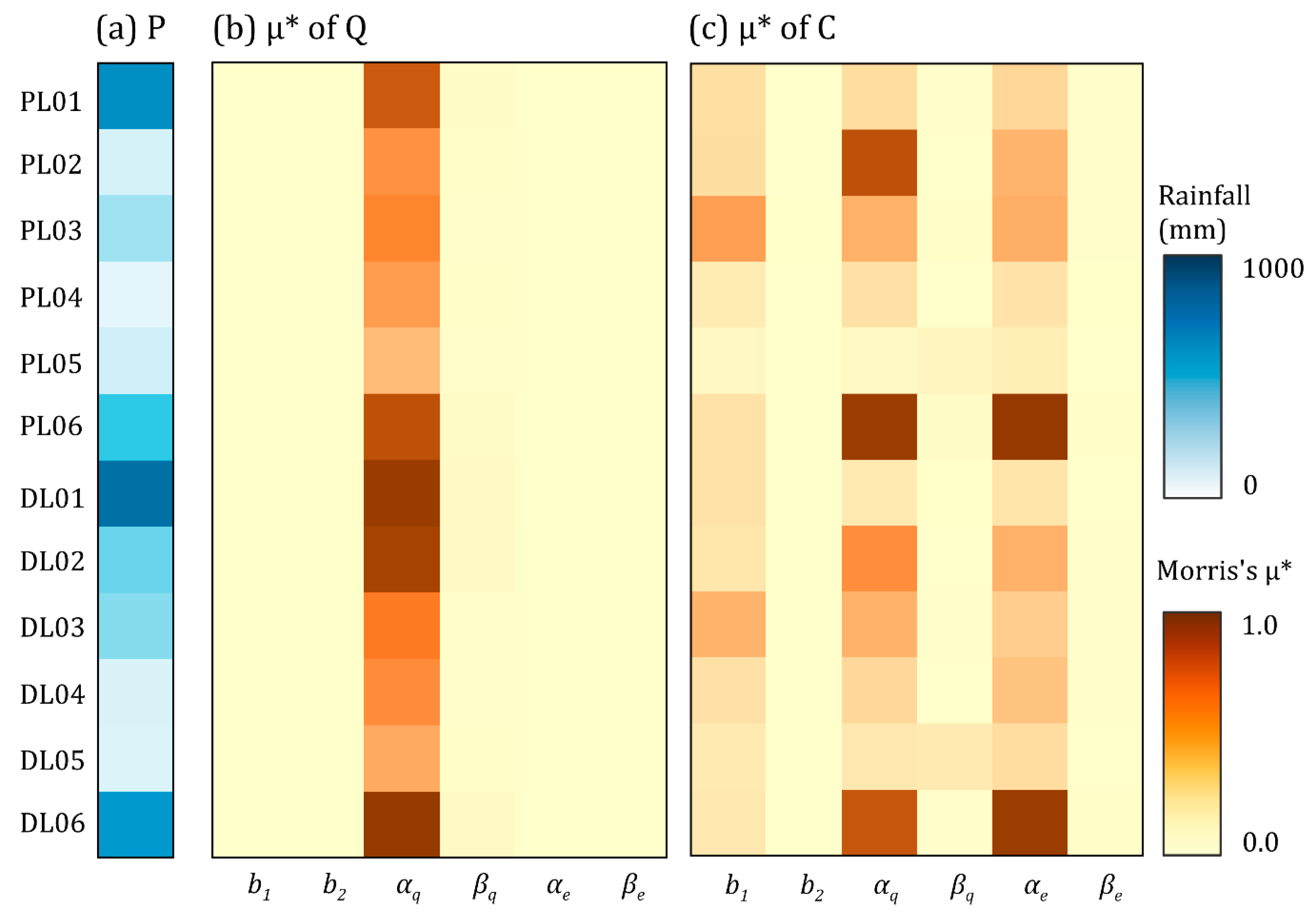
3.3. Parameter Sensitivity

The global parameter sensitivity analysis for streamflow and tracer modules is illustrated in Figure 3 using scaled Morris’s μ value. Parameter α_q, used for the runoff transfer function, was determined as the only sensitive parameter in the streamflow module, and it appeared to increase with the total rainfall, whereas other parameters were not as sensitive in the streamflow module. In the tracer module (Figure 3c), two parameters, b₁ and b₂, depict the separation of the fraction of the effective rainfall into event water and the decaying effect, respectively, (Table 1) but only b₁ was sensitive. Since the change of δ¹⁸O in the streamflow is governed by the rainwater volume, the fraction of the effective rainfall certainly dominated the tracer module, whereas parameter b₂ was less sensitive, because it only controlled how much of the previous effective rainfall would recharge into event water. Parameters α_q and α_e were dominant parameters in the tracer module; however, the scale parameters, β_q and β_e, were insensitive. Besides, the three sensitive parameters (b₁, α_q, and α_e) seemed irrelative to the total rainfall.

4. Discussion

4.1. Rapid Response from Rainfall to Streamflow during Typhoons

Conceptually, the variability of δ¹⁸O in streamwater is assumed to be dampened and lagging behind rainfall due to rainfall-runoff transfer [35], whereas our δ¹⁸O in streamwater almost synchronized with that in rainwater, with R² = 0.73 (Figure 2), indicating a rapid rainfall-runoff transfer. The MTT_ew in the two mesoscale catchments varying from 2.3 to 10.9 h (Table 4), was as short as that in microscale catchments (less than 100 ha). For example, Weiler et al. [16] applied the TRANSEP model onto a steep catchment in New Zealand (Maimai M8 with a drainage area of 0.17 km² and an average slope of 34°) and found that the MTT_ew was approximately 10 h. McGuire and McDonnell [36] derived an averaged MTT_ew of 20 h in a 0.11 km² catchment with a slope of 37° in Oregon via the same model. We further compiled eight previous studies, which all applied the TRANSEP model onto catchments with different environmental settings (see Supplementary Material, Table S3) to examine the relationship between catchment size and MTT_ew and F_ew. The MTT_ew ranged from 1.0 to 93.8 h and the F_ew from 0.01 to 0.77 (Figure 4a,b) with the catchment size between 0.002 and 100 km². The MTT_ew in both gentle and steep catchments seems to increase with catchment size that is less than 10 km². The MTT_ew is relatively short for large rainstorms, and a long MTT_ew only appears in small and moderate rainstorms. The relationship becomes vague as the intensity of rainstorms increases. One possible interpretation is that heavy rainstorms, which disperse rainwater more directly and quickly, can boost the hydrological connectivity between hillslope and the stream, particularly for fractured catchments, and thus reduce the transit time [36,37]. Furthermore, the relationship between F_ew and catchment size is shown in Figure 4b. Generally, F_ew vaguely increases with catchment size and rainfall intensity in our compilation although F_ew increases with rainfall intensity in a tropical small lowland catchment, Puerto Rico [38]. Collectively, there is no simple and clear relationship between either catchment size, slope, or rainstorm size and MTT_ew and F_ew. The unclear relationship with catchment size implies that perhaps intrinsic catchment structure (e.g., flow-path length, flow-path gradient, or subsurface permeability) might be a more important control than catchment size, not only for MTT of total streamflow [14,15,39] but also for MTT_ew. Further work is needed to identify the controls on catchment structure and rainstorm characteristics. This identification would be helpful for upscaling from observed microscale studies to unobserved meso or macroscale catchments.

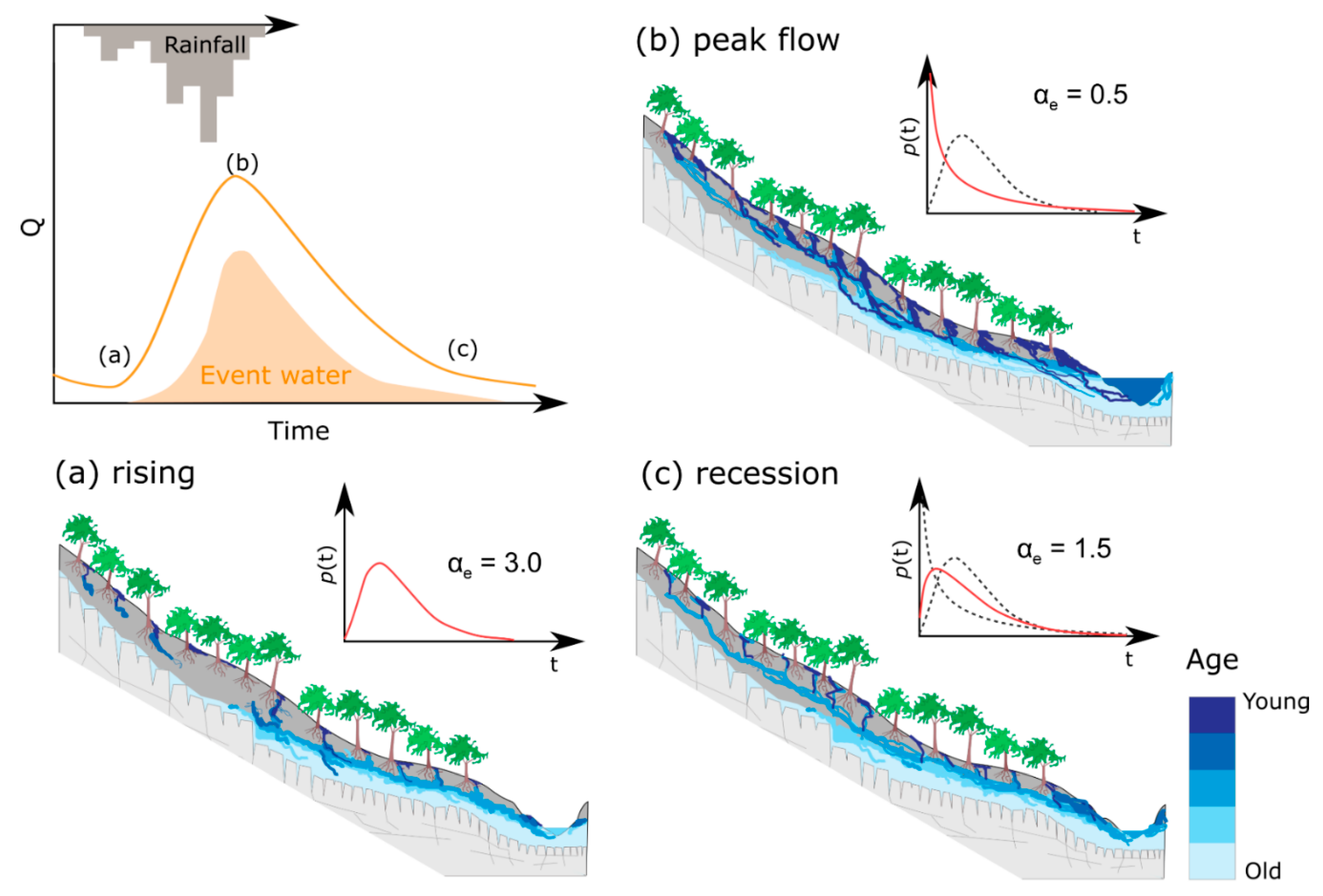
4.2. Rainfall Control on the Variability of MTT_ew, F_ew, and α_e

The correlation coefficient matrix of parameters against hydrometric factors (Supplementary, Table S4) presents that the average rainfall intensity (RI_avg), maximum 3-h rainfall amount (P_max3h), and antecedent wetness (AP_7day) are highly relevant to the TTD-associated parameters. Since RI_avg and P_max3h are highly collinear, RI_avg and AP_7day, the two well-known indicators in the literature [24,25], were selected for discussion.

The relationship of MTT_ew with RI_avg is presented in Figure 5a. MTT_ew exponentially decreases with the increase of RI_avg (R² = 0.39, p-value < 0.06) for all AP_7day conditions, indicating that high rainfall intensity can effectively shorten the MTT_ew at event scale, though the statistical significance is marginal. McGuire and McDonnell [36] studied the runoff dynamics in the H.J. Andrew Experimental Forest in Oregon through successive rainstorms and concluded that the subsurface contributing areas extend far upslope during rainstorms, and the reduction of MTT_ew was therefore implied. The extended subsurface contributing area and the enhanced hydrological connectivity help to interpret our exponential decreases of MTT_ew in relation to RI_avg. On the other hand, the statistically-positive correlation of F_ew against RI_avg indicates that the higher the rainfall intensity, the more the event water is transported (Figure 5b, R² = 0.55, p-value < 0.01). Brown et al. [40] argued that an increase of event water fraction delivered from throughfall and shallow subsurface flow is directly related to rainfall intensity. Recently, Kirchner [41] developed an age-tracking benchmark model to show that high antecedent wetness increases the partitioning of rainfall that reaches the stream resulting in high F_ew. However, Muñoz-Villers and McDonnell [42] applied the TRANSEP model onto tropical montane catchments and found that the event water contribution decreased with an increasing antecedent wetness condition. They argued that if high permeability of soils and lithologic substrate can lead to vertical rainfall percolation and recharge of deeper layers, the rainfall-runoff responses could be dominated by groundwater discharge, rather than shallow lateral pathways. Although our wet antecedent wetness cases (blue dots) also show a decrease of F_ew with the increase of antecedent wetness, it would be hasty to jump to a conclusion with only three sampled cases. The controversy of F_ew responding to antecedent wetness, therefore, still needs further investigation, including thinking about the fracture systems in lithologic substrates, as Gabrielli et al. [43] suggested.

From a modelling perspective, the relationship between α_e of gamma distribution and rainfall intensity presents an exponentially-negative regression (Figure 5c, R² = 0.50, p-value < 0.05) in both wet and dry antecedent conditions. Generally, larger α_e values can only be found when rainfall intensity is less than ~10.0 mm h⁻¹. When higher rainfall intensity exceeds 10.0 mm h⁻¹, α_e would decrease below 1.0. When rainfall transports without dispersion, like plug flow, a large α would be determined. For a catchment with α = 1, a linear or well-mixed reservoir could be identified. As α < 1, the catchment is more likely to exhibit a relatively high degree of nonlinearity (i.e., high initial peaks and longer tails in the TTDs), indicating preferential flow-paths are rapidly activated and quickly route water to the catchment outlet. Therefore, the parameter, α, can be used to depict the mixing degree during runoff generation and/or the catchment storage [10,44] to infer how event water is mixed in the event water reservoir. In our cases, with increase in rainfall intensity, the α_e reduced from 3.0 to 0.5, indicating that the mixing varied from plug flow, through well-mixed, to preferential flow. The emergence of preferential flow may imply that the rapid lateral subsurface flow from rainwater without well-mixing with groundwater dominated the MTT_ew in large rainstorms.

4.3. Transition of Parameter Sensitivity during Typhoons

Generally, parameter sensitivity provides identifiability information of parameters to understand the interaction of model functions, and more complicatedly, it may vary in response to different conditions (e.g., landscape setting or flow regimes). Parameter α_q is the only sensitive parameter in the streamflow module, while α_q, α_e, and b₁ are the sensitive parameters in the tracer module (Figure 3). Therefore, α_q is the only parameter which simultaneously regulates both the streamflow and the tracer module in our environmental setting, which is steep and humid. Since α_q regulates the shape of the runoff transfer function, it is not surprising that it gets more sensitive with the increase of rainfall input. Although α_q is also a sensitive parameter in the tracer module, no distinct relationship between α_q and the total rainfall could be found. In other words, the δ¹⁸O responses have a complicated interaction within the tracer module, which mimics the mixing processes and flow-path change via temporal rainfall allocation (wetness condition). This involves two more sensitive parameters, α_e, and b₁.

Since parameter sensitivity likely varies depending on different wetness conditions, the change in parameter sensitivity within an event should be demonstrated for understanding the dynamics of the model and the underlying processes, such as the timing of dominance of a given parameter or a process. Therefore, the normalized Morris’s μ with 12-h moving windows at an hourly step for three parameters, α_q, α_e, and b₁, are undertaken for the intra-event variability in parameter sensitivities (Figure 6 and Table S5). Event PL05 (small event) and PL06 (large event) with a similar dry antecedent condition are taken as examples. The small event resulted in a small event water fraction and the peak of event water fraction coincided with the streamflow peak. By contrast, the large event lead to a large event water fraction and the peak of event water fraction came sooner than the streamflow peak. Parameter b₁ in the small event became sensitive with time, whereas it became dormant in the large event. Parameter α_q was not very sensitive in the small event, but its response to streamflow was significant. As for α_e, it got sensitive with streamflow, formed a plateau around the peak flow, and then shrank along with the recession in the small event. However, in the large event, the sensitivity of α_e surged to form a plateau before the peak of streamflow, sustained the plateau through the peak flow and then diminished. The above comparison signifies: (1) parameter sensitivity is case-dependent, and (2) the chronosequent parameter sensitivity may present a clockwise or counter-clockwise hysteresis or linear response. As storm magnitude increases, the counter-clockwise hysteresis occurs. Hydrologic processes such as the bedrock detention storage hypothesis [45], bedrock exfiltration, or lagged contribution due to enhanced connectivity in upslope regions [46] may explain the observed hysteretic pattern between rainfall and α_e sensitivity.

Collectively, a conceptual diagram of our hypothesis, which shows how transit time distribution of event water varies during an event in fractured catchments, is presented (Figure 7). The variation of TTD_ew and water ages in catchment storage is described in three hydrograph stages: (1) The rising limb stage—event water infiltrates into near subsurface to partially replace the pre-event water stored in the subsurface, which slowly flows to stream and thus yields a damped TTD_ew.; (2) The peak flow stage—event water tends to connect existing effective flow-paths, known as preferential flows, from upslopes and riparian areas, resulting in a sharp TTD_ew. The event water traveling through preferential flows with high mobility leads to a younger streamwater age. (3) The recession stage—as rainfall diminishes and event water reduces, partial pre-event water can use the effective flow-paths and, consequently, the streamwater age becomes older and the TTD_ew turns from sharp to damped. In attempting to clarify the function of event water in the subsurface, one should either select the storage response function [10,18], or incorporate the rainfall pulse to adjust parameter [23] to further explore the controlling factors of MTT_ew. Our temporal parameter sensitivity shows that the MTT_ew and F_ew during an event are the integrated responses to the competition of rainfall input against storage through vertical permeability. For small events (the storage capacity is larger than the rainfall input), the event rainfall is able to infiltrate into the storage via fractures so that few event water and plug flow can be inferred (Figure 5). In that case, the pre-event water dominates the hydrograph and thus the MTT_ew controller α_e exerts its function after the peak flow (Figure 6). By contrast, rainfall of large events, which exceeds the storage capacity, can rapidly generate more event water via preferential flow but not overland flow, which was rarely witnessed during our sampling in typhoon periods. This may imply the emergence of subsurface flow that transports plenty of event water. To conclude, we suggest the concept of “the competition of rainfall input against the storage” and the switching to subsurface flow during a rainstorm can be taken into the time-variant parameterization in model development in the future.

5. Conclusions

Mean transit time of event water (MTT_ew) is highly associated with flow-paths underground and has earned much attention over the past decade, but has rarely been studied in steep and fractured catchments where flow-path shifting during typhoons is relevant to many biogeochemical processes. Our MTT_ew (in the drainage area of 79 and 110 km²) varied around 2–11 h, in the same order of magnitude with the MTT_ew in small-scale catchments of 0.02–8.8 km², indicating catchment size may not be the first-order control on MTT_ew in catchment area spanning from 0.02 to 100 km². Catchment structure (e.g., flow-path length, flow-path gradient, and subsurface permeability) might be a more important control than catchment size. From the compilation of our datasets, either MTT_ew or F_ew has a complex relationship with catchment size, slope, or rainstorm size. The unclear relationship with catchment size implies that perhaps intrinsic catchment structure (e.g., flow-path length, flow-path gradient, and subsurface permeability) might be a more important control on MTT_ew and F_ew. Focusing on our cases, it is suggested that MTT_ew exponentially decreases with the increase of rainfall intensity because large rainstorms activate preferential flow processes and hence enhance the hillslope–stream connectivity. Intriguingly, antecedent wetness baffles the positive relation between rainfall intensities and F_ew, indicating the mixing mechanism of pre-event and event water still remains a puzzle that warrants further investigation.

Inter-event sensitivity analysis demonstrated that in our case, parameters b₁, α_q, and α_e were most sensitive to the tracer simulation performance. The shape parameter α_e has been seen as a proxy of event water drainage behavior from plug flow, through the well-mixed, to preferential flow when its value decreases. In our study, the αe reduced from 3.0 to 0.5 as rainfall intensity magnified, which suggests αe being from plug flow to preferential flow. Meanwhile, αe echoed the streamflow within an event, implying that the soil wetness is relevant to α_e. Collectively, the MTT_ew and F_ew during an event are integrated responses to the competition of rainfall input against storage through vertical permeability. Further study should address: (1) how to mimic this competition into time-variant parameterization for presenting the mixing change from plug flow to preferential flow which is particularly required for estimating streamflow transit time in steep and fractured catchments and (2) how to identify water ages of preferential flow and plug flow during various rainstorms.

References

1. Stewart, M.; McDonnell, J.J. Modeling Base Flow Soil Water Residence Times from Deuterium Concentrations. Water Resour. Res. 1991, 27, 2681–2693. [Google Scholar] [CrossRef]
2. Stark, C.; Stieglitz, M. The sting in a fractal tail. Nature 2000, 403, 493–495. [Google Scholar] [CrossRef] [PubMed]
3. Maher, K.; Chamberlain, C.P. Hydrologic Regulation of Chemical Weathering and the Geologic Carbon Cycle. Science 2014, 343, 1502–1504. [Google Scholar] [CrossRef] [PubMed]
4. Kirchner, J.W. A double paradox in catchment hydrology and geochemistry. Hydrol. Process. 2003, 17, 871–874. [Google Scholar] [CrossRef]
5. Kirchner, J.W.; Feng, X.; Neal, C. Fractal stream chemistry and its implications for contaminant transport in catchments. Nature 2000, 403, 524–527. [Google Scholar] [CrossRef] [PubMed]
6. Turner, J.; Albrechtsen, H.J.; Bonell, M.; Duguet, J.P.; Harris, B.; Meckenstock, R.; McGuire, K.; Moussa, R.; Peters, N.; Richnow, H.H.; et al. Future trends in transport and fate of diffuse contaminants in catchments, with special emphasis on stable isotope applications. Hydrol. Process. 2006, 20, 205–213. [Google Scholar] [CrossRef]
7. Burns, D.A.; Vitvar, T.; McDonnell, J.J.; Hassett, J.; Duncan, J.; Kendall, C. Effects of suburban development on runoff generation in the Croton River basin, New York, USA. J. Hydrol. 2005, 311, 266–281. [Google Scholar] [CrossRef]
8. Buttle, J.M.; Hazlett, P.; Murray, C.; Creed, I.F.; Jeffries, D.; Semkin, R. Prediction of groundwater characteristics in forested and harvested basins during spring snowmelt using a topographic index. Hydrol. Process. 2001, 15, 3389–3407. [Google Scholar] [CrossRef]
9. McGuire, K.J.; McDonnell, J.J. A review and evaluation of catchment transit time modeling. J. Hydrol. 2006, 330, 543–563. [Google Scholar] [CrossRef]
10. Harman, C. Time-variable transit time distributions and transport: Theory and application to storage-dependent transport of chloride in a watershed. Water Resour. Res. 2015, 51, 1–30. [Google Scholar] [CrossRef] [Green Version]
11. Soulsby, C.; Birkel, C.; Geris, J.; Dick, J.; Tunaley, C.; Tetzlaff, D. Stream water age distributions controlled by storage dynamics and nonlinear hydrologic connectivity: Modeling with high-resolution isotope data. Water Resour. Res. 2015, 51, 7759–7776. [Google Scholar] [CrossRef] [PubMed] [Green Version]
12. Jasechko, S.; Kirchner, J.W.; Welker, J.M.; McDonnell, J.J. Substantial proportion of global streamflow less than three months old. Nat. Geosci. 2016, 9, 126–129. [Google Scholar] [CrossRef]
13. McGuire, K.J.; McDonnell, J.J.; Weiler, M.; Kendall, C.; McGlynn, B.L.; Welker, J.M.; Seibert, J. The role of topography on catchment-scale water residence time. Water Resour. Res. 2005, 41, W05002. [Google Scholar] [CrossRef]
14. Tetzlaff, D.; Seibert, J.; McGuire, K.J.; Laudon, H.; Burns, D.A.; Dunn, S.M.; Soulsby, C. How does landscape structure influence catchment transit time across different geomorphic provinces? Hydrol. Process. 2009, 23, 945–953. [Google Scholar] [CrossRef]
15. Hale, V.C.; McDonnell, J.J. Effect of bedrock permeability on stream base flow mean transit time scaling relations: 1. A multiscale catchment intercomparison. Water Resour. Res. 2016, 52, 1358–1374. [Google Scholar] [CrossRef]
16. Weiler, M.; McGlynn, B.L.; McGuire, K.J.; McDonnell, J.J. How does rainfall become runoff? A combined tracer and runoff transfer function approach. Water Resour. Res. 2003, 39, 315. [Google Scholar] [CrossRef] [Green Version]
17. McDonnell, J.J.; McGuire, K.J.; Aggarwal, P.; Beven, K.J.; Biondi, D.; Frampton, A.; Dunn, S.; James, A.L.; Kirchner, J.W.; Kraft, P.; et al. How old is streamwater? Open questions in catchment transit time conceptualization, modelling and analysis. Hydrol. Process. 2010, 24, 1745–1754. [Google Scholar] [CrossRef] [Green Version]
18. Botter, G. Catchment mixing processes and travel time distributions. Water Resour. Res. 2012, 48, W05545. [Google Scholar] [CrossRef]
19. Herman, J.D.; Kollat, J.B.; Reed, P.M.; Wagener, T. From maps to movies: High-resolution time-varying sensitivity analysis for spatially distributed watershed models. Hydrol. Earth Syst. Sci. 2013, 17, 5109–5125. [Google Scholar] [CrossRef] [Green Version]
20. Huang, J.-C.; Milliman, J.D.; Lee, T.-Y.; Chen, Y.-C.; Lee, J.-F.; Liu, C.-C.; Lin, J.-C.; Kao, S.-J. Terrain attributes of earthquake- and rainstorm-induced landslides in orogenic mountain Belt, Taiwan. Earth Surf. Process. Landforms 2017, 42, 1549–1559. [Google Scholar] [CrossRef]
21. Zehetner, F.; Vemuri, N.L.; Huh, C.-A.; Kao, S.-J.; Hsu, S.-C.; Huang, J.-C.; Chen, Z.-S. Soil and phosphorus redistribution along a steep tea plantation in the Feitsui reservoir catchment of northern Taiwan. Soil Sci. Plant Nutr. 2008, 54, 618–626. [Google Scholar] [CrossRef]
22. Lin, T.-C.; Shaner, P.-J.L.; Wang, L.-J.; Shih, Y.-T.; Wang, C.-P.; Huang, G.-H.; Huang, J.-C. Effects of mountain tea plantations on nutrient cycling at upstream watersheds. Hydrol. Earth Syst. Sci. 2015, 19, 4493–4504. [Google Scholar] [CrossRef] [Green Version]
23. Hrachowitz, M.; Soulsby, C.; Tetzlaff, D.; Malcolm, I.A.; Schoups, G. Gamma distribution models for transit time estimation in catchments: Physical interpretation of parameters and implications for time-variant transit time assessment. Water Resour. Res. 2010, 46, W10536. [Google Scholar] [CrossRef] [Green Version]
24. Klaus, J.; McDonnell, J.J. Hydrograph separation using stable isotopes: Review and evaluation. J. Hydrol. 2013, 505, 47–64. [Google Scholar] [CrossRef]
25. Segura, C.; James, A.L.; Lazzati, D.; Roulet, N.T. Scaling relationships for event water contributions and transit times in small-forested catchments in Eastern Quebec. Water Resour. Res. 2012, 48, W07502. [Google Scholar] [CrossRef]
26. Huang, J.-C.; Yu, C.-K.; Lee, J.-Y.; Cheng, L.-W.; Lee, T.-Y.; Kao, S.-J. Linking typhoon tracks and spatialrainfall patterns for improving flood lead time predictions over a mesoscale mountainous watershed. Water Resour. Res. 2012, 48, W09540. [Google Scholar] [CrossRef]
27. Jakeman, A.; Hornberger, G.M. How much complexity is warranted in a rainfall-runoff model? Water Resour. Res. 1993, 29, 2637–2649. [Google Scholar] [CrossRef]
28. Maloszewski, P.; Rauert, W.; Trimborn, P.; Herrmann, A.; Rau, R. Isotope hydrological study of mean transit times in an alpine basin (Wimbachtal, Germany). J. Hydrol. 1992, 140, 343–360. [Google Scholar] [CrossRef]
29. Lu, M.-C.; Chang, C.-T.; Lin, T.-C.; Wang, L.-J.; Wang, C.-P.; Hsu, T.-C.; Huang, J.-C. Modeling the terrestrial N processes in a small mountain catchment through INCA-N: A case study in Taiwan. Sci. Total. Environ. 2017, 593, 319–329. [Google Scholar] [CrossRef]
30. Kling, H.; Fuchs, M.; Paulin, M. Runoff conditions in the upper Danube basin under an ensemble of climate change scenarios. J. Hydrol. 2012, 424, 264–277. [Google Scholar] [CrossRef]
31. Madsen, H. Automatic calibration of a conceptual rainfall–runoff model using multiple objectives. J. Hydrol. 2000, 235, 276–288. [Google Scholar] [CrossRef]
32. Morris, M.D. Factorial Sampling Plans for Preliminary Computational Experiments. Technometrics 1991, 33, 161–174. [Google Scholar] [CrossRef]
33. Pianosi, F.; Beven, K.; Freer, J.; Hall, J.W.; Rougier, J.; Stephenson, D.B.; Wagener, T. Sensitivity analysis of environmental models: A systematic review with practical workflow. Environ. Model. Softw. 2016, 79, 214–232. [Google Scholar] [CrossRef]
34. Herman, J.D.; Kollat, J.B.; Reed, P.M.; Wagener, T. Technical Note: Method of Morris effectively reduces the computational demands of global sensitivity analysis for distributed watershed models. Hydrol. Earth Syst. Sc. 2013, 17, 2893–2903. [Google Scholar] [CrossRef] [Green Version]
35. Lyon, S.W.; Desilets, S.L.E.; Troch, P.A. Characterizing the response of a catchment to an extreme rainfall event using hydrometric and isotopic data. Water Resour. Res. 2008, 44, W06413. [Google Scholar] [CrossRef]
36. McGuire, K.J.; McDonnell, J.J. Hydrological connectivity of hillslopes and streams: Characteristic time scales and nonlinearities. Water Resour. Res. 2010, 46, W10543. [Google Scholar] [CrossRef] [Green Version]
37. Jencso, K.G.; McGlynn, B.L.; Gooseff, M.; Wondzell, S.M.; Bencala, K.E.; Marshall, L. Hydrologic connectivity between landscapes and streams: Transferring reach- and plot-scale understanding to the catchment scale. Water Resour. Res. 2009, 45, W04428. [Google Scholar] [CrossRef] [Green Version]
38. Schellekens, J.; Scatena, F.; Bruijnzeel, L.; Van Dijk, A.; Groen, M.M.A.; Van Hogezand, R.J.P. Stormflow generation in a small rainforest catchment in the Luquillo Experimental Forest, Puerto Rico. Hydrol. Process. 2004, 18, 505–530. [Google Scholar] [CrossRef]
39. Asano, Y.; Uchida, T. Flow path depth is the main controller of mean base flow transit times in a mountainous catchment. Water Resour. Res. 2012, 48, W03512. [Google Scholar] [CrossRef]
40. Brown, V.A.; McDonnell, J.J.; Burns, D.A.; Kendall, C. The role of event water, a rapid shallow flow component, and catchment size in summer stormflow. J. Hydrol. 1999, 217, 171–190. [Google Scholar] [CrossRef]
41. Kirchner, J.W. Quantifying new water fractions and transit time distributions using ensemble hydrograph separation: Theory and benchmark tests. Hydrol. Earth Syst. Sci. 2019, 23, 303–349. [Google Scholar] [CrossRef] [Green Version]
42. Muñoz-Villers, L.E.; McDonnell, J.J. Runoff generation in a steep, tropical montane cloud forest catchment on permeable volcanic substrate Runoff generation in a steep, tropical montane cloud forest catchment on permeable volcanic substrate. Water Resour. Res. 2012, 48, W09528. [Google Scholar] [CrossRef] [Green Version]
43. Gabrielli, C.P.; McDonnell, J.J.; Jarvis, W. The role of bedrock groundwater in rainfall–runoff response at hillslope and catchment scales. J. Hydrol. 2012, 450, 117–133. [Google Scholar] [CrossRef]
44. Berghuijs, W.; Kirchner, J.W. The relationship between contrasting ages of groundwater and streamflow. Geophys. Res. Lett. 2017, 44, 8925–8935. [Google Scholar] [CrossRef] [Green Version]
45. McDonnell, J.J. Where does water go when it rains? Moving beyond the variable source area concept of rainfall-runoff response. Hydrol. Process. 2003, 17, 1869–1875. [Google Scholar] [CrossRef]
46. Lehmann, P.; Hinz, C.; McGrath, G.; Van Meerveld, I.; McDonnell, J.J. Rainfall threshold for hillslope outflow: An emergent property of flow pathway connectivity. Hydrol. Earth Syst. Sci. 2007, 11, 1047–1063. [Google Scholar] [CrossRef] [Green Version]
Figure 1. (a) Location, topographic, and monitoring network of Ping-Lin (PL) and Da-Lin (DL) catchments. The red triangles are streamwater sampling sites and streamflow gauges. The yellow and purple squares represent the location of rain gauges and rainwater sampling sites, respectively. (b) Boring logs from BHP-34 drilled in the near stream site and from B-4 drilled in the hillslope site.
Water 12 01169 g001
Figure 2. Simulations of streamflow and δ18O of PL05 and PL06. The hyetograph and hydrograph of PL05 (a,b) and PL06 (d,e). The cyan- and gray-shaded areas in (b,e) represent uncertainty intervals of total flow and event water simulations from representative parameter sets, respectively. The observed and simulated δ18O of PL05 (c) and PL06 (f).
Water 12 01169 g002
Figure 3. Sensitivity metric for parameters in streamflow and tracer module against total rainfall. Total rainfall (a) of the individual catchment-event. Scaled Morris’s μ value of parameters in streamflow (b) and tracer (c) module, which are derived from their corresponding root mean squared error (RMSE).
Water 12 01169 g003
Figure 4. Scatter plots of catchment against MTTew (a) and Few (b) in compiled literature (Table S3) with different catchment average slopes. The circles and square dots represent gentle and steep catchments, respectively. The blue, cyan, and green color of dots represent the rainfall intensity. The error bars represent the maximum and minimum boundaries of representative simulations.
Water 12 01169 g004
Figure 5. Scatter plots of RIavg against MTTew (a), Few (b), and αe (c) for all catchment-events. The orange and blue dots represent that antecedent 7-day rainfall (AP7day) of 30 mm is set as the criterion for presenting dry and wet condition, respectively. Note that the regression line in plot (b) is only fitted with orange dots. The drainage behaviors of event water corresponding to αe are labelled on (c). The error bars represent the maximum and minimum boundaries of representative simulations.
Water 12 01169 g005
Figure 6. Time-varying sensitivity calculated with the tracer for three sensitive parameters in Figure 3. The rainfall-runoff simulation for PL05 (a) and PL06 (b). The scaled sensitivity indices (Morris’s μ* value) are calculated for a 12-h moving window with a 1 h time step for PL05 (c) and PL06 (d). The dashed vertical lines represent the timing of flow peak.
Water 12 01169 g006
Figure 7. The hypothesis of event water movement during typhoon periods with the change of TTDs. The three hydrograph stages are: rising stage (a), peak flow (b), and recession (c). The TTDs demonstrate the behaviors of event water yields corresponding to the three stages.
Water 12 01169 g007