Porous Medium Typology Influence on the Scaling Laws of Confined Aquifer Characteristic Parameters


Department of Civil Engineering, University of Calabria, via P. Bucci, Cubo 42B, 87036 Arcavacata di Rende (CS), Italy
*
Author to whom correspondence should be addressed.
Water 2020, 12(4), 1166; https://doi.org/10.3390/w12041166
Submission received: 4 March 2020
/
Revised: 14 April 2020
/
Accepted: 17 April 2020
/
Published: 19 April 2020
(This article belongs to the Special Issue Modeling of Flow and Transport in Saturated and Unsaturated Porous Media)
Abstract
:An accurate measurement campaign, carried out on a confined porous aquifer, expressly reproduced in laboratory, allowed the determining of hydraulic conductivity values by performing a series of slug tests. This was done for four porous medium configurations with different granulometric compositions. At the scale considered, intermediate between those of the laboratory and the field, the scalar behaviors of the hydraulic conductivity and the effective porosity was verified, determining the respective scaling laws. Moreover, assuming the effective porosity as scale parameter, the scaling laws of the hydraulic conductivity were determined for the different injection volumes of the slug test, determining a new relationship, valid for coarse-grained porous media. The results obtained allow the influence that the differences among the characteristics of the porous media considered exerted on the scaling laws obtained to be highlighted. Finally, a comparison was made with the results obtained in a previous investigation carried out at the field scale.
1. Introduction
Among the parameters’ characterizing aquifers, certainly the hydraulic conductivity is one of the most meaningful and useful for the description of the flow and mass transport phenomena in porous media. The scalar behavior of this parameter, namely the variation of the values that this assumes with the scale parameter variation, was the object of numerous studies that highlighted and verified this behavior under different conditions and contexts. Specifically, several scientists and researchers showed a tendency to increase the value of the hydraulic conductivity (K) with the scale [1,2,3,4,5,6,7,8,9,10]. The causes of this behavior are mainly attributed to the heterogeneity of the porous medium, constituting the aquifer in question. On small scales, it manifests itself mainly through the shape and size of the pores, while, on the larger scales, it is manifested through the tortuosity, the interconnection and the continuity of the pores and interstitial canaliculi [11,12,13,14]. This last aspect shows how important the influence of the considered porous medium structure is, namely the characteristics of the relative intergranular spaces, of their shape and size and of the relative granulometric assortment. All these characteristics are generally summarized in the parameters describing the texture of the porous medium under examination and in other parameters, such as porosity (n), which is often assumed as a representative parameter, thus assuming great importance. Specifically, many authors refer to the effective porosity (ne) so as to take into account also the interconnection conditions of the voids, which have a decisive influence on water flow and on the mass transport phenomena that are located in them [10,15]. Moreover, it seems possible, albeit in an uncertain manner, to affirm the existence of a scalar behavior even for the porosity; however, this does not always consist in a tendency to increase the porosity with the scale but sometimes with a decreasing trend with increasing of this, as verified by some researchers [16,17]. In any case, considerable caution should be used in asserting the existence of a scalar behavior of porosity, due to the great complexity of the phenomena that determine the influence of the heterogeneity of the porous medium [18]. In some studies, the porosity—or, more appropriately, the effective one—is assumed as a scale parameter [7,10]. In this way, it is possible to identify the modalities of the hydraulic conductivity variation when the porosity changes and the corresponding scaling law constitutes a valid alternative to the numerous empirical and semi-empirical formulas based on the grain size distribution [19,20,21,22,23]. The importance of determining a scaling law for a given parameter is also due to the fact that this allows identification of the distribution of the considered parameter in the spatial context taken into consideration, avoiding the use of traditional geostatistical methods [24,25]. However, in the experimental verification of the scaling behavior of the hydraulic conductivity, it is necessary to verify that the significant values of this parameter were obtained in contexts and in conditions to guarantee a correct comparison, namely under identical flow conditions. This is particularly important if a series of K values measured at different scales, in the field and in the laboratory on samples of porous media, are considered. In fact, on the latter, the measure generally supplies the vertical hydraulic conductivity value, while field tests are used to obtain the value of the horizontal one. Therefore, in such cases, the K values must be standardized, trying to obtain the values of the horizontal hydraulic conductivity using suitable methods for the measurements carried out on soil samples in laboratory, often based on the knowledge of the anisotropy of the porous medium under examination [10,23,26,27].
The aim of the present study consists in an experimental investigation on the variation modalities of the scaling laws of the parameters examined, namely hydraulic conductivity and effective porosity, according to the variation of the porous medium, constituting the artificial confined aquifer. The aquifer used in the investigation was purposely realized in a metallic sand box in the GMI Laboratory of the University of Calabria. Within the sand box, four confined aquifers were reproduced in successive phases with different types of porous media and all subjected to careful granulometric analysis to determine their main characteristic parameters. On each of these aquifers, several K measurements were carried out using slug tests, then using a characteristic measurement method of field. Therefore, after having separately verified the scaling behavior of K and ne, this last parameter was assumed as a scale parameter, identifying a single K variation law when ne, namely the porous medium, changes. The scaling law thus obtained represents a new relation able to give the value of K, known the value of ne, within the porous media examined and those of similar characteristics, therefore describable also in terms of grain size distribution. The usefulness of a relationship of this type is evident, as it allows users to make a fast and reliable estimate of the hydraulic conductivity, even if limited to the ambit, although vast, of the investigated soils and taking into account some conditions and restrictions specified below.
In this regard, it should be noted that the investigation ambit of this study certainly concerns the coarse-grained porous media, with a predominantly sandy matrix but, also, that it is delimited by the particular scale considered here. In fact, this scale, intermediate between the characteristice of the laboratory samples and that of the field, is of particular interest in numerous applications and has so far it was poorly investigated. Therefore, the results obtained in the present experimental investigation, even if of significant interest, are valid exclusively for coarse grained aquifers and at the mesoscale considered here.
In the following, after describing the experimental device and the characteristics of the porous media used to reproduce the four different aquifers, the measurement methods of the parameters taken into consideration are briefly recalled. Afterwards, with an extensive discussion, the results obtained are reported in terms of K and ne scaling laws and a new variation law of K with ne performing the appropriate comparisons with the results obtained using the grain size distribution methodologies.
2. Materials
2.1. Experimental Set-Up, Equipment and Tests Execution
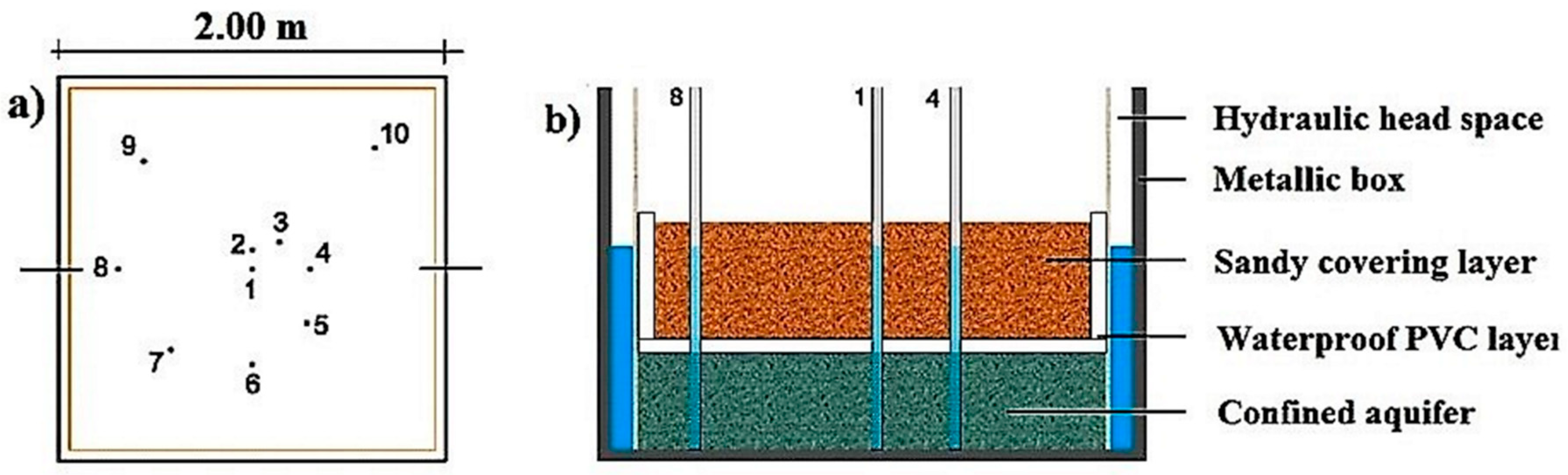
A series of slug tests in a 3D-confined aquifer were performed at the Laboratory “Grandi Modelli Idraulici” of the Department of Civil Engineering of the University of Calabria (Italy), using a 2-m-long, 2-m-wide and 1-m-deep metal box, as schematized in Figure 1. Ten PVC wells with a diameter D equal to 2.8 cm were located in the metal box, as shown in Figure 2.
All the wells were completely penetrating, with openings on the pipe walls throughout the thickness of the confined formation and covered in the same area with a geotextile layer in order to avoid soil materials entering into the wells. Well No. 1 (the central one) was considered as the injection well, while the other nine observation wells were distributed in different directions and at increasing distances from the center, as shown in Figure 1a. Four different heterogeneous configurations of porous media were considered covering the entire area of the metal box starting from the bottom and with a thickness of the formation, ts, as shown for each configuration in Table 1. Table 1 also shows the undisturbed hydraulic head related to the injection well. In order to ensure the confined formation, a thin impermeable plastic panel was laid down over each configuration and then covered with additional sandy material. The impermeability of the confined formation was verified by means of some preliminary tests [25]. In order to guarantee a constant hydraulic head condition during the tests, a perimetric chamber was built along the metal box lateral boundaries, and the perimetric chamber was connected with two external loading reservoirs. More details are given in [28]. Several slug tests were performed for each soil configuration using an injection volume V into the central well of 0.03 L, 0.04 L, 0.06 L, 0.07 L, 0.08 L and 0.09 L, respectively. The initial undisturbed hydraulic head varied between 0.32 m and 0.38 m to ensure that the confined formation remained under pressure, and the complete restoration of the initial loading conditions between tests was always verified [28,29]. In order to measure head changes during the slug tests, 10 submersible transducers, model Druck PDCR1830 (for more details, see [30,31,32]), were positioned at the bottom of each well. The pressure data were recorded using a measurement frequency of 100 Hz and filtered using the Mexican hat wavelet transform to eliminate the experimental high-frequency noise, as suggested by the authors of [28].
2.2. Soil Configurations
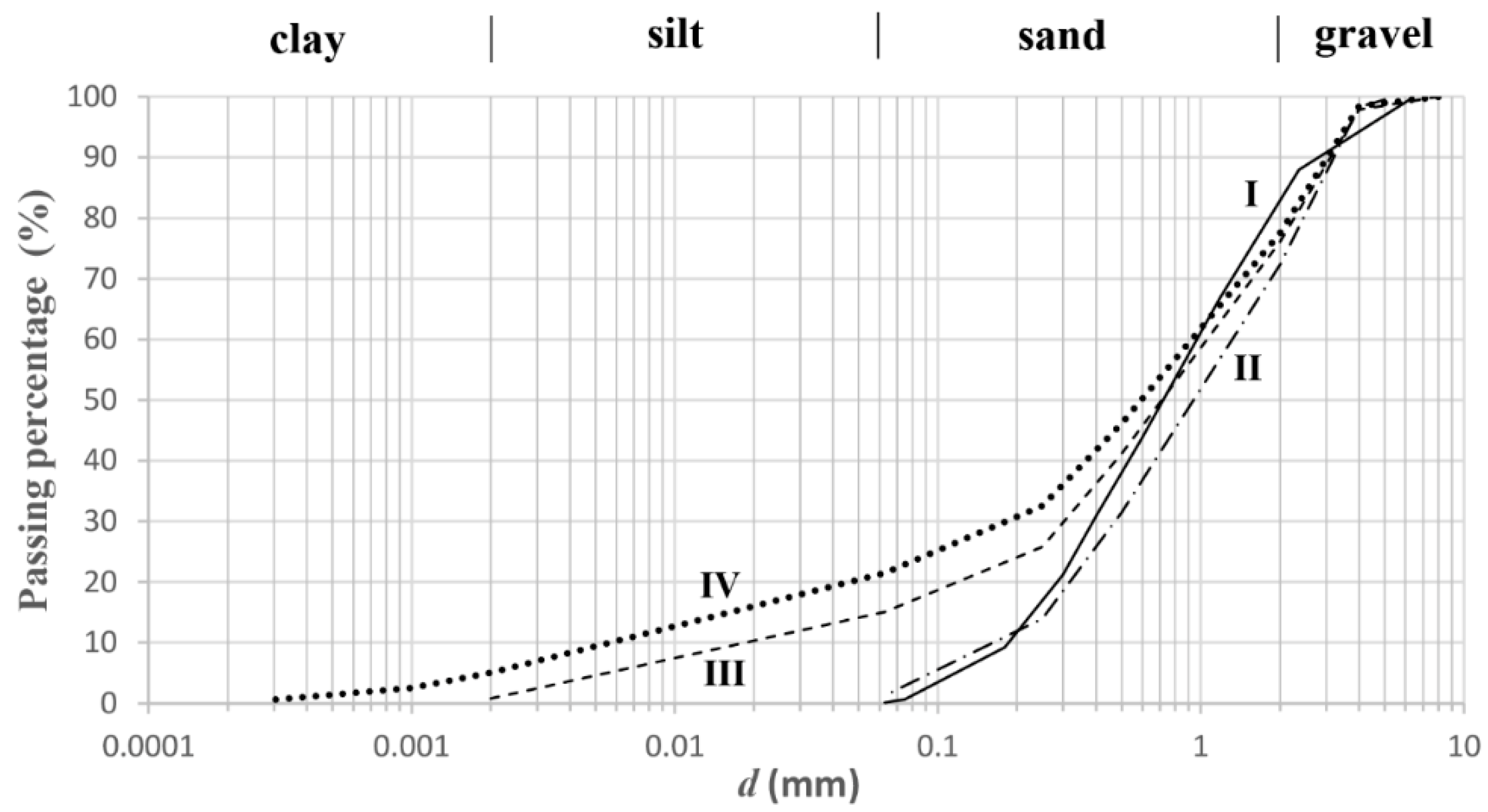
The measurement campaign of the hydraulic conductivity, consisting of conducting slug tests, was repeated for all the four types of porous media used to build, in subsequent times, the confined aquifer taken into consideration. Each of the four porous media considered was subjected to a careful granulometric analysis, leading to the determination of their main granulometric and textural characteristics. Table 2, for each of the four porous media considered, shows the respective percentages of the granulometric components; the diameter value d10 was assumed as an effective diameter, the uniformity coefficient (U = d60/d10) and the values of total and effective porosity [24,33]. The graph in Figure 3 shows the granulometric curves characterizing the four types of porous media used for the construction of the corresponding confined aquifers. The highest gravel content is present in the porous medium of type II with 27.70%, while the lower content is relative to that of the type I with 12.01%. Regarding the sand, the highest content was found in the first porous medium type, which contains about 88%, while the lower content of this component is found in the porous medium of type IV with 56.10%. The maximum silt content was found in the configuration of the type IV with 16.40%, while the minimum was found in the configuration type I with 0.60%.
The clay is absent in almost all the configurations taken into consideration, except the type IV, where a modest amount equal to 5% of this component was found. Therefore, all the porous media considered are predominantly coarse-grained. Specifically, the type I porous medium can be defined as sandy, while the remaining three types are predominantly sandy, with a non-negligible amount of gravel. As a result, the presence of silt is certainly not significant. Moreover, it is possible to notice that, from the configurations I to IV, the diameter d10 tends to decrease, varying from 0.19 mm to 0.0055 mm, while the uniformity coefficient tends to increase, going from 5.21 to 163.63. The total porosity for type I configuration assumes the highest value, equal to 37.6%, while, for the other three configurations, it assumes lower and comparable values, ranging between 27.3% and 29.3%. The effective porosity tends to increase, passing from configuration I to IV, assuming values ranging between 5.60% and 19%.
3. Methods
3.1. Data Analysis
The hydraulic head values detected during slug tests were appropriately processed by the method suggested by the authors of [34]. The boundary conditions imposed by this method are as follows:
where H is the variation in the well of the hydraulic head from the undisturbed value (L), H0 the initial variation in the well of the hydraulic head (L), h the variation of the hydraulic head from the undisturbed value at a generic radial distance (L), rw the effective radius of well screen (L), rc the effective radius of well casing (L), r the radial distance (L), t the time (T), Kr the component of the hydraulic conductivity in radial direction (LT−1), Ss the specific storage (L−1) and B the thickness of the aquifer (L). The relationships (1) and (2) state that at time t = 0, the hydraulic head variation is zero everywhere outside the well and equal to H0 inside the well. Moreover, the relationship (3) establishes that, for r approaching to infinity, the variation of the hydraulic head approaches zero, while, for the relation (4), the hydraulic head in the immediate vicinity of the well is equal to that inside it for t > 0. Finally, the boundary condition (5) requires compliance with the continuity principle for incoming and outgoing flows from the aquifer—well system. In compliance with these boundary conditions, the mathematical model suggested by the authors of [34] is expressed by the following relation:
valid for the homogeneous aquifer, unsteady state flow, instantaneous injection and negligible well losses [34,35].
3.2. Scaling Analysis
The scaling behavior of a hydraulic parameter characterizing a porous aquifer can certainly be represented by different types of laws. However, the most commonly used law for this purpose is certainly the power type, represented by the following relation:
where P is the parameter examined (in the case of the hydraulic conductivity (LT−1)), x is the scale parameter (as the representative scale dimension (L)), a is a parameter that takes into account the structure and the heterogeneity of the porous medium (having the dimensions to ensure congruence) and b (-) is the scaling index (also called crowding index), which is related to the type of flow in the porous medium [5]. The use of a power-type law to represent the scaling behavior of a parameter requires the fulfillment of the so-called lacunarity condition. This condition consists in identifying minimum and maximum cut-off limits within the range of values of the parameter under examination, within which the hydrological process remains correctly defined. This implies that the scaling parameter considered is representative of a scale-invariant phenomenon [36]. These cut-off limits can be determined identifying, within the investigation context, the range showing the maximum value of the determination coefficient (R2), as treated in numerous studies in the literature [9,25,36]. In the following, the scale invariance of the phenomenon and the condition of lacunarity were assumed, and on this basis, the scaling behaviors of K and ne were verified using Equation (7). Initially, this equation was used assuming as scaling parameter the radius of influence (R), the values of which were measured experimentally for each value of K. However, it must be clearly understood that, with the term radius of influence, one means the dimension that characterizes the confined aquifer volume involved in the measurement of the parameter under examination—for example, K—taking into account that the measured value of this parameter is representative only of this volume and that it changes if this varies. This volume can be assumed to be of cylindrical shape, and an estimate of its amplitude can be provided by R. Subsequently, the same effective porosity was assumed as a scaling parameter. Specifically, the total porosity was measured in the laboratory using the densiometric method by the following relationship [37,38]:
where ρbulk is the bulk mass density (ML−3) and ρgrain the particle mass density (ML−3), while the effective one, considering the saturated medium, was obtained based on the following relationship:
where V (L3) is the total volume and Vw (L3) the portion of the water volume which cannot be drained by gravity [39].
3.3. Grain Size Analysis
Empirical and semiempirical formulas are often used to determine hydraulic conductivity by measuring some parameters characterizing the granulometric distribution of the medium. The parameters include porosity and, specifically with reference to the water flow in the porous medium, the effective porosity. Therefore, by carrying out a careful grain size analysis of the medium considered, namely determining the main granulometric parameters, it is possible to determine the corresponding hydraulic conductivity value using the formula considered more suitable to the specific case [22,23,40]. To determine K, it is possible to use a scaling law of the type of Equation (7), assuming ne as a scaling parameter. Furthermore, other empirical and semiempirical formulas are based on the grain size distribution theory. These formulas commonly follow the general model of [40], represented by the following equation:
where K is the hydraulic conductivity of saturated porous media (LT−1), ne is the effective porosity (-), C a general coefficient (-), ν the kinematic viscosity (L2T−1), g the acceleration of gravity (LT−2), f(ne) the porosity function defining the relationship between the real and modeled porous media and de the effective grain diameter (L).
4. Results and Discussion
For each of the slug tests carried out on the four considered configurations, a careful analysis of the hydraulic head values was conducted, determining the K values by the method of the authors of [34]. The four soil configurations considered are evidently homogeneous, as requested by the authors of [34] method reported previously. Even if the soil configurations considered are constituted by different types of porous media, the overall composition of each configuration remains uniform throughout the aquifer volume. Although these configurations can be defined as homogeneous, as highlighted previously, an evident heterogeneity remains in the aquifer due to the different dimensions and shape of the grains, their arrangement within the porous medium and, consequently, the different interconnections of the voids, as well as to the variation of tortuosity. Especially in field investigations but also in laboratory models if there are doubts about the homogeneity of the porous medium and to better investigate some particular aspects, such as the interconnection of the pore voids, the carrying out of tracer tests and geophysical tests can be very useful [41,42,43]. The hydraulic conductivity values thus obtained are shown in Table 3, for each configuration and for all the values of the injection volume considered; Table 3 also reports the corresponding radius of influence values determined experimentally during the tests. For each data set of K and R given in Table 3, a careful statistical analysis was carried out, reporting the main parameters in Table 4.
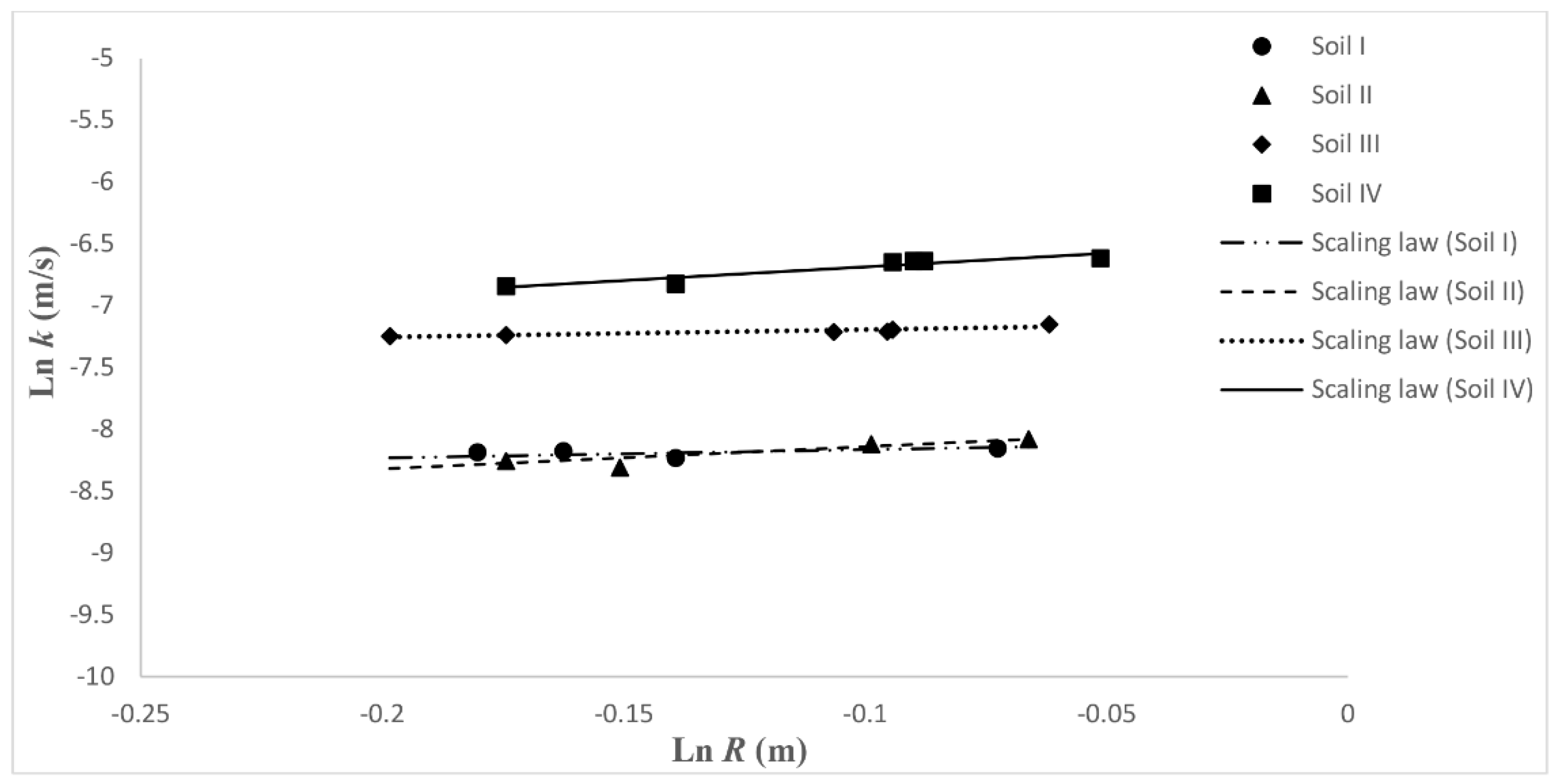
The K values vary between a minimum equal to 1.36 × 10⁻⁴ m/s (configuration of the type II) and a maximum value 1.34 × 10⁻³ m/s (configuration of the type IV). The mean value varies between a minimum value of 2.45 × 10⁻⁴ m/s in the configuration of the type II and a maximum equal to 1.24 × 10⁻³ m/s in that of the type IV. The variance (VAR) assumes always very low values, with an order of magnitude between 10−10 and 10−8. The standard deviation (SD) assumes values with order of magnitude between 10−5 and 10−4. The standard error (SE) 10−5 shows values with an order of magnitude of 10−5. The variation coefficient (VC) shows values with an order of magnitude between 10−2 and 2.56 × 10⁻¹. Similarly, the mean value of R is variable from 0.799 m to 0.90 m, with the variance (VAR) variable between a minimum equal to 0.001 and a maximum equal to 0.015, the standard deviation (SD) variable between a minimum equal to 0.039 and a maximum equal to 0.123, the standard error (SE) variable between a minimum equal to 0.016 and a maximum equal to 0.050 and the coefficient of variation (VC) variable between a minimum value of 0.043 and a maximum value of 0.154. Afterwards, assuming the radius of influence as the scale parameter, it was possible to identify the variation modalities of K with R for each of the four porous medium configurations taken into consideration, determining the corresponding scaling laws by means of power-type relations, according to Equation (7), which, for the specific case, is given by the following relation:
The parameters a and b of the four scaling laws thus obtained are shown in Table 5. From Table 5, it is possible to notice that the values of the parameter a relative to the configurations of types I and II are very close and that the determination coefficient values are high for all four configurations considered. The maximum value of R2 is relative to configuration II.
The logarithmic graph of Figure 4 shows the trend of the four scaling laws of Table 5, limited to the variation range of R common to all four configurations considered, namely delimited by the values 0.59 m and 0.95 m.
The graph shown in Figure 4 shows that the scaling laws related to the configurations of the types I and II are very similar, as expected, since the relative granulometric compositions do not show substantial differences, as evidenced by Table 2 and Figure 3.
Furthermore, as shown by the data of Table 5 and Figure 4, the type I and II configurations presented much lower hydraulic conductivity values than those of the type III and IV configurations, which are characterized by a more varied granulometric assortment, with lower quantities of sand and higher percentages of silt and gravel. The type I and II configurations, with a fairly uniform particle size composition, mainly consisting of sand, with a limited percentage of gravel and a negligible amount of silt, also highlight an evident scaling behavior, with an increase of K increasing the radius of influence (R), assumed as a scale parameter. In turn, the type III configuration gave lower K values than type IV, which has a larger granulometric assortment, with a higher silt content, with a limited presence of clay and a quantity of gravel comparable with that of the type III configuration.
After investigating the scaling behavior of hydraulic conductivity, it was also possible to investigate the scaling behavior of effective porosity due to the importance that this parameter has for flow and mass transport in porous media. Therefore, the ne values relative to each of the configurations taken into consideration, shown in Table 2, were correlated with the radii of influence (R) identified experimentally for each injection volume considered for the slug tests, as shown in Table 3. The corresponding scaling laws, determined according to relation (7), are represented in the specific case by the following relation:
are defined by the parameters shown in Table 6.
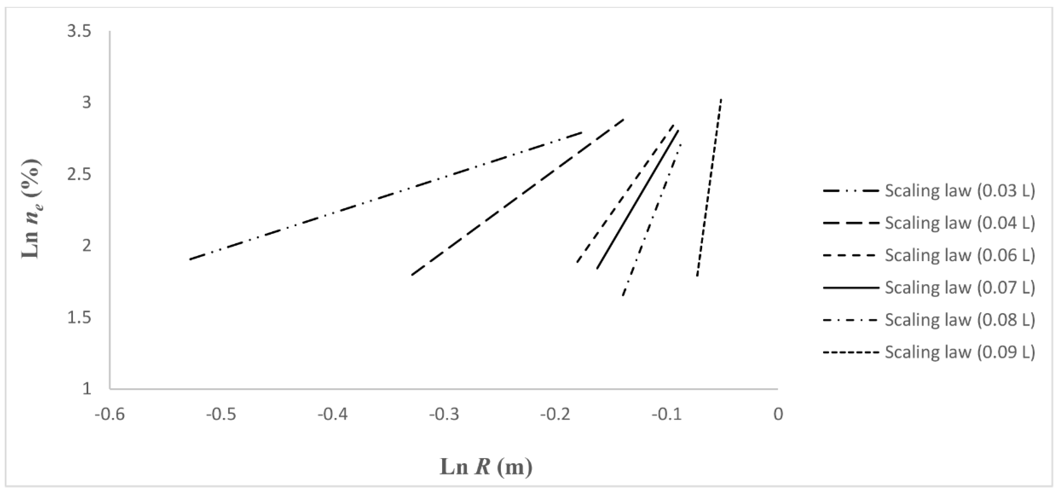
Table 6 shows that the a and b parameter values increase as the injection volume increases, while the values of R2 are all high, varying between a minimum value of 0.795, related to the injection volume of 0.08 L and a maximum value of 0.958, relative to the injection volume of 0.09 L. Figure 5 shows the trends of the scaling laws related to the injection volumes considered for the slug tests. The R2 values shown in Table 6 and the trends of the scaling laws represented by Equation (12) and obtained for the injection volumes considered, confirm the existence of a positive scaling behavior of ne, namely that there is an increase of ne as R increases. Furthermore, the graph in Figure 5 shows that the R values, measured for the four configurations considered, fall within ranges which have amplitudes tending to decrease with increasing the injection volume considered for slug tests.
This circumstance is highlighted, on the double logarithmic graph in Figure 5, by the increase in the slope of the straight lines representing the scaling law described by Equation (12), passing from that relating to the injection volume of 0.03 L to that relative to the volume of 0.09 L. This could mean that the substantial differences, which can be observed for small injection volumes, tend to decrease in a clear manner when the value of these volumes increases. Since each of the four configurations taken into consideration is characterized by a single value of ne, in order to investigate the variation of K with ne, it was decided to assume a fixed value of the radius of influence R and to verify the corresponding variation modalities of the parameters under examination, assuming as a scale parameter ne, to determine the following scaling law:
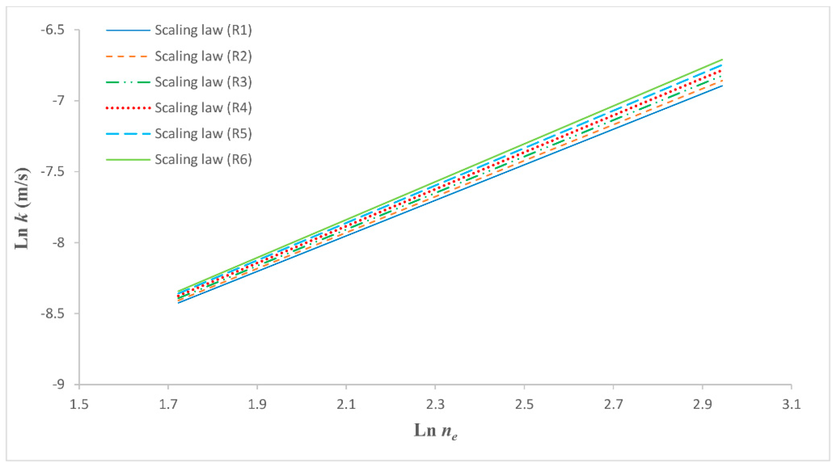
This was done for a congruous number of R values equal to six, set within the overlapping interval of the scaling laws expressed by Equation (11) for all four configurations considered, represented by parameters a and b of Table 5 and shown in Figure 4. The fixed R values are equal to: R1 = 0.8400 m, R2 = 0.8573 m, R3 = 0.8746 m, R4 = 0.8931 m, R5 = 0.9112 m and R6 = 0.9305 m. For each of these values, the scaling law represented by the relation (13) was determined, and the related parameters a, b and R2 are shown in Table 7.
The contents of Table 7 show that the parameter a values differ slightly, varying between 2.38 × 10⁻⁵ and 2.54 × 10⁻⁵. Additionally, the parameter b assumes very similar values, varying between 1.2513 and 1.3361, while R2 assumes always high values, between a minimum of 0.859 and a maximum of 0.910. Furthermore, it can be seen that, as the fixed value of R increases, the parameter a tends to decrease and b tends to increase, as well as R2. Figure 6 shows the trends of the scaling laws represented by Equation (13) for the six fixed values of R, according to what is reported in Table 7.
The results obtained confirm the scalar behavior of K vs. ne already found in previous studies [7,10]. As already noted, analyzing the data shown in Table 7, Figure 6 also shows that the six scaling laws representing the variation of K with ne for the different fixed R values are very similar, even if they show a not marked tendency to accentuate the relative differences. In fact, Figure 6 highlights the tendency to diverge the straight lines representing the scaling laws for the fixed R values on the double logarithmic graph of this figure. On the basis of these results, an attempt was made to determine a single scaling law, also of the type of Equation (13), which allows to determine the variation of K with ne for all the injection volumes and for the four soils, with the configurations taken into consideration and all those similar to these. For this purpose, determining the mean values of the parameters a and b of the individual scaling laws, the only law representative of the four configurations considered was identified, defined by the following parameter values:
a = 2.46 × 10⁻⁵ and b = 1.29
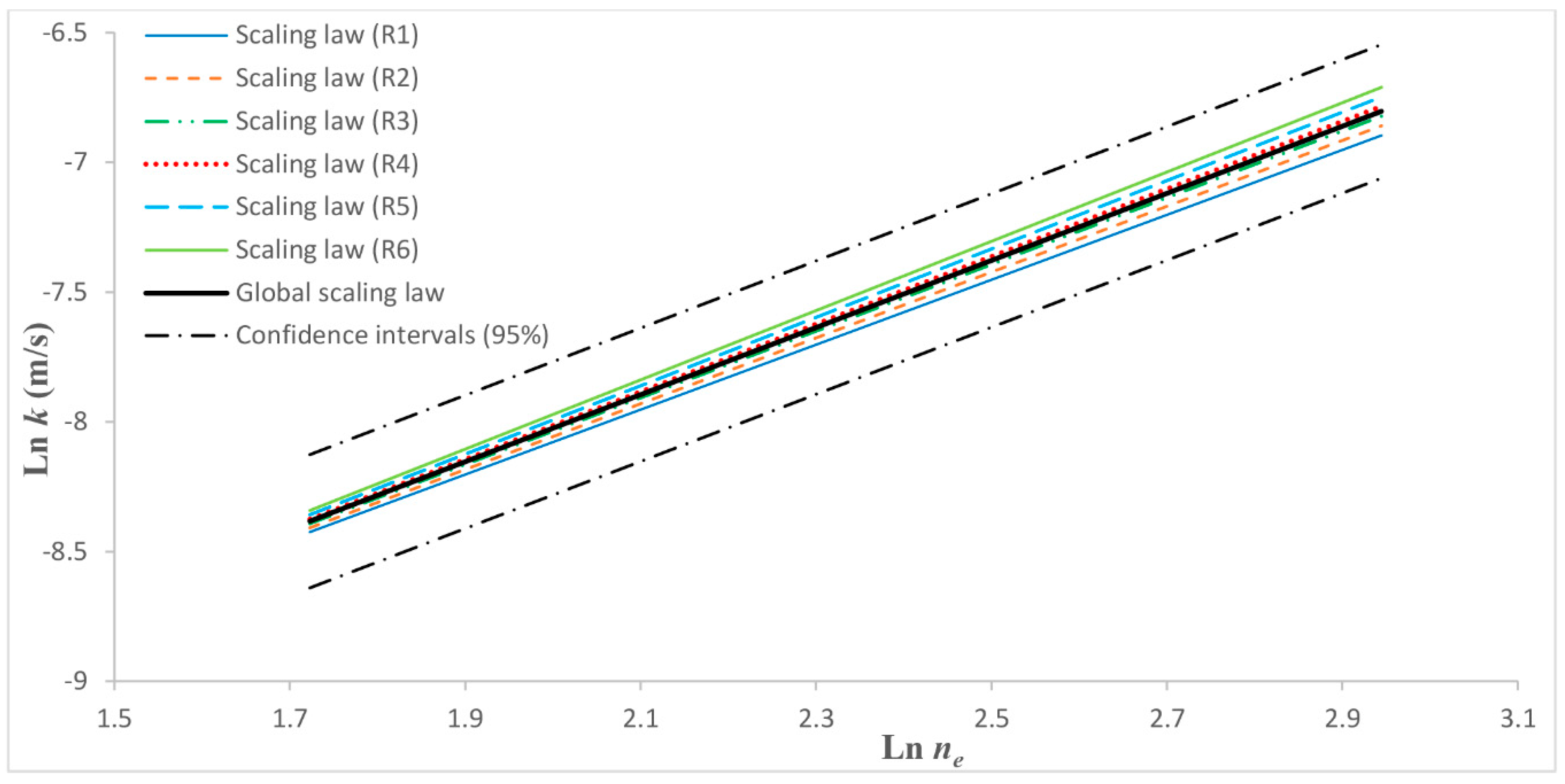
In the graph shown in Figure 7, in addition to the scaling laws represented by Equation (13) relative to each input volume considered, it also reports the only global scaling law valid for all porous media with characteristics similar to those of porous media considered in the configurations examined. Furthermore, the corresponding 95% confidence intervals are also shown on the graph of Figure 7, relative to this global scaling law.
The double logarithmic graph in Figure 7 shows that the line representing the global scaling law is almost overlapping those of the scaling laws obtained with the R3 and R4 radii of influence. Furthermore, the other straight lines, representing the scaling laws relating to the remaining R values, are thickened to that representative of the global scaling law, and they are all inside the 95% confidence intervals. The global scaling law, represented by Equation (13) and specified by the parameters provided by (14), expresses the variability of K vs. ne. Since ne is a characteristic parameter of the porous medium, it was considered appropriate also to consider the empirical and semi-empirical equations deriving from the grain size distribution. Therefore, the general model of [40] was considered. With reference to this model, described by Equation (10), the global scaling law defined above by relations (13) and (14) can also be explained by the following expression:
where d10 (L) is the particle size for which 10% of the sample are finer than and the meaning of other symbols was already specified. This law, represented by Equation (15), presents a field of validity defined by 5.5 × 10⁻³ mm ≤ d10 ≤ 0.19 mm. Although it is evident that relation (14) is simpler and more immediate than relation (15), it is undeniable that, in the presence of fluids other than water, or for values of d10 not falling within the validity range of the (15); both the previous relations must be calibrated again, determining new values of the coefficients a and b of the relation (14) and also of the coefficient C and ne index of relation (10). Equation (15) was compared to one of the best-known relationships following the model of [40], which is the [19,20] equation which, valid for d10 < 3 mm and not appropriate for clayey soils [44], falls within the validity range of this investigation. The graph in Figure 8 shows the trends of both these variation laws.
From the graph of Figure 8, it is possible to notice that, even if the two laws taken into consideration are very similar, that of Kozeny-Carman presents a lower slope for the same investigation range—that is, a variation of K contained in a smaller range. In Figure 8, another scaling law is also reported, similar to that represented by relations (14) and (15), previously determined by [10] with different field measurement methods (pumping tests, slug tests and tracer tests) carried out on a natural confined aquifer, with a thickness of about 44 m, consisting of a porous medium identifiable as sandy loam. High percentages of silt and a constant presence of clay, which became relevant approaching the impermeable bottom layer, made the porosity of the porous medium significantly lower than the values of the configurations considered in the present investigation, with values contained within 10%. On the contrary, in the study of [10], the hydraulic conductivity resulted significantly higher due to the different external loads induced on the aquifer by the tests and by the relevant volumes of aquifer involved in the field measurements not comparable with those taken into consideration in the present investigation, despite these last measurements were carried out by slug tests, namely with a proper measurement method of field. The substantial differences between the aquifers considered in the two studies do not allow a correct comparison of the results but enable the significant differences that emerge investigating at different scales, such as those of the field and intermediate between the laboratory and field, to be highlighted and taken into consideration in the present analysis.
5. Conclusions
The scaling behavior verification of the main hydrogeological parameters that characterize an aquifer, such as the hydraulic conductivity, and the determination of the corresponding scaling laws are of great importance for the description of the flow and mass transport phenomena occurring in it. However, on these phenomena, also other parameters characterizing the structure of the porous medium have a great influence, depending on the shape and size of the grains, their assortment and disposal—such as, for example, the porosity. In fact, even these aspects and, therefore, the parameters that describe them, characterize the porous medium, determining its heterogeneity. Since a saturated porous medium heterogeneity is assumed at the base of the so-called scaling effect and the manner in which this occurs at different scales both influences and determines the scaling behavior of the various parameters characterizing an aquifer, it is clear that one cannot disregard a careful analysis of these aspects in the study of the aforementioned phenomena interesting a specific aquifer. Specifically, the present study investigated the influence that the variation of the parameters characterizing the porous medium structure exerts on the scaling behavior of the hydraulic conductivity taken as a parameter representative of the hydrogeological aspects considered within the aquifer. For the K measurement, it was preferred to carry out slug tests, rather than pumping tests, as in previous studies [25], for greater simplicity. In fact, with the experimental laboratory device considered here, to maintain constant pumping with very small flow rates, a necessary condition for ensuring compliance with the boundary conditions of the data analysis method under consideration is very difficult. On the contrary, it is easier to set, even in large numbers, the injection volumes for the slug tests, respecting the initial and boundary conditions. Obviously, since the slug tests are notoriously single-well tests, unlike pumping tests, the K values determined by this type of test are related to the same injection well. Therefore, the measured value of the radius of influence, taken as the characteristic parameter of the aquifer volume affected by the test, was fixed as scale parameter. The experimental investigation was carried out on four different configurations of a confined aquifer built in a metal box in the GMI Laboratory of the University of Calabria. All four aquifer configurations in question can be defined as coarse-grained, with a predominantly sandy matrix and different amounts of gravel and silt, while a modest amount of clay was present only in the configuration of type IV. For the parameter K, the existence of the scaling behavior was verified for all four configurations considered. Given the particular scale of investigation, which can be defined as intermediate between those of the laboratory and field, it is reasonable to assume that the scaling laws obtained for the different configurations considered, represented by the relation (11) and defined by the values of parameters a and b shown in Table 5, are affected by the influence of heterogeneity with the modalities with which this manifests itself on the two opposite scales: of the laboratory and field. Moreover, since the porous media related to the configurations considered were characterized by a single value of the effective porosity, the available values of this parameter were only four. Therefore, the investigation on the scaling behavior of ne, assuming as scale parameter R, was made for each injection volume used in the execution of the slug tests. As shown by the data of Table 6 and by Figure 5, the scaling behavior of ne is also verified for all the cases examined, with an increase of this parameter with the increase of R. Furthermore, by decreasing the injection volume and the ne value in the investigation interval, the variation range of R tends to decrease. Due to the particular scale of investigation, even the scaling laws determined for ne are affected by the influence of heterogeneity with the modalities mentioned above. Afterwards, ne was assumed as a scaling parameter, and the scaling law (13) was determined for each injection volume considered. Since the laws obtained were very similar, as evidenced by the values of Table 7 and Figure 6, a single scaling law was identified, with a level of significance of 5%, representative of all the individual laws relating to each injection volume. The values of parameters a and b of this global scaling law, represented in Figure 7, are given by relation (14). Obviously, even in this case, the scaling laws reported in Table 7 and, consequently, also the one defined by relation (14) are influenced by the heterogeneity with the modalities induced by the particular scale of investigation. Relation (14) represents, therefore, a new law, K = K(ne), valid within the porous media investigated and in those with similar characteristics, namely that can be defined as coarse-grained. To highlight further the importance of the parameters characterizing the structure of porous media, the new law, K = K(ne), represented by Equation (14), was also written in terms of grain size analysis, obtaining, on the model of [40], Equation (15), which is very similar to that obtainable with the model of [19,20] and valid always for coarse-grained aquifers.
Certainly, it should be kept in mind that the results obtained in the present investigation are valid only in the context of the experimentation carried out, i.e., for coarse-grained porous media with prevailing sand content. However, it is necessary to recognize that the investigation range considered is unquestionably very wide and is able to cover a relevant part of the application field.
The great influence exerted by the different configurations considered for the porous medium and the relative representative parameters were also highlighted, comparing Equation (15) with that obtained from Fallico (2014) for a porous medium mainly consisting of sand and loam, also taking into account the different measurement conditions, even though using field measurement methods on the experimental device built in the laboratory. The present investigation has allowed further verification of the scaling behavior of K, and the results were obtained on a perfectly known experimental device and, above all, at an intermediate scale between that of the laboratory, such as that defined by the representative dimensions of the soil samples on which the tests are generally carried out, and that of the field. This circumstance implies that, at this intermediate scale, the heterogeneity, to which the scaling behavior of the parameters under examination is attributed, manifests its influence both through the shape and dimensions of the voids, characteristic modes of the laboratory scale, and through the connectivity and the tortuosity of the canaliculi, its own mode of the field scale. This is evidenced by the fact that K tends to not only increase ne but also increase the injection volume, namely approaching the flow conditions proper to those of the field scale, as shown by the laws of Table 7 and highlighted in Figure 6 and in Figure 7. Understanding and verification of these mechanisms is of fundamental importance for a correct description of the flow and transport phenomena in porous media, for which it is desirable to increase the experimental research on these topics, with the acquisition of a greater quantity of significant data. Furthermore, it should be pointed out that the use of grain size analysis is able to provide alternative relationships, also easy to use but only usable on the basis of the structural characteristics of the considered porous medium and certainly not always able to easily define the spatial distribution of the parameter under examination, which is possible, however, using the scaling laws, thus avoiding the need to use of the traditional geostatistical methods. Therefore, even if the scaling laws depend on fewer variables than the relationships provided by the grain size analysis, they also have a limited validity range. In fact, for scaling laws, this validity range is represented by the particular scale for which they were determined. With reference to this study, the scaling laws determined on the basis of Equations (11), (12) and (13) are valid exclusively within the mesoscale of interest defined above.
This limitation of the validity of the scaling laws determined in the present study, of course, adds up to that imposed by the particular porous media taken into consideration to constitute the aquifer configurations examined—that is, substantially, to the coarse-grained porous media with prevailing sand content.
Regarding the effective hydraulic conductivity, the transition from local to large scale was studied and defined [45]. However, it is not a topic considered in the present study, which is purely experimental and concerns exclusively the mesoscale defined above, or considered of great interest.
The present experimental study, in addition to providing new data which are useful to the scientific community, further verifies the existence of hydraulic conductivity scaling behavior, highlighting the existence of an analogous behavior also for the effective porosity.
In particular, relationship (14) proposed here, of very simple use and valid for all types of porous media investigated, is of great utility for potential users, presenting the great advantage of immediately having reliable indications about the value of hydraulic conductivity, albeit with all the limitations previously highlighted.
Author Contributions
Conceptualization, C.F.; methodology, C.F., A.L. and F.A.; formal analysis, C.F., A.L. and F.A.; investigation, A.L.; data curation, F.A.; writing—original draft preparation, C.F., A.L. and F.A.; writing—review and editing, C.F., A.L. and F.A.; supervision, C.F. All authors have read and agreed to the published version of the manuscript.
Funding
This research received no external funding
Acknowledgments
The authors thank the unknown reviewers for their useful comments and suggestions.
Conflicts of Interest
The authors declare no conflicts of interest.
References
- Clauser, C. Permeability of crystalline rocks. EOS Trans. Am. Geophys. Union 1992, 73, 237–238. [Google Scholar] [CrossRef]
- Neuman, S.P. Universal scaling of hydraulic conductivity and dispersivities in a geologic media. Water Resour. Res. 1990, 26, 1749–1758. [Google Scholar] [CrossRef]
- Rovey, C.W.; Cherkauer, D.S. Scale dependency of hydraulic conductivity measurements. Groundwater 1995, 33, 769–780. [Google Scholar] [CrossRef]
- Schulze-Makuch, D.; Cherkauer, D.S. Method developed for extrapolating scale behavior. EOS Trans. Am. Geophys. Union. 1997, 78, 3. [Google Scholar] [CrossRef] [Green Version]
- Schulze-Makuch, D.; Cherkauer, D.S. Variations in hydraulic conductivity with scale of measurement during aquifer tests in heterogeneous, porous, carbonate rocks. Hydrogeol. J. 1998, 6, 204–215. [Google Scholar] [CrossRef]
- Schulze-Makuch, D.; Carlson, D.A.; Cherkauer, D.S.; Malik, P. Scale dependency of hydraulic conductivity in heterogeneous media. Groundwater 1999, 37, 904–919. [Google Scholar] [CrossRef]
- Fallico, C.; De Bartolo, S.; Troisi, S.; Veltri, M. Scaling analysis of hydraulic conductivity and porosity on a sandy medium of an unconfined aquifer reproduced in the laboratory. Geoderma 2010, 160, 3–12. [Google Scholar] [CrossRef]
- Fallico, C.; Vita, M.C.; De Bartolo, S.; Straface, S. Scaling effect of the hydraulic conductivity in a confined aquifer. Soil Sci. 2012, 177, 385–391. [Google Scholar] [CrossRef]
- Fallico, C.; De Bartolo, S.; Veltri, M.; Severino, G. On the dependence of the saturated hydraulic conductivity upon the effective porosity through a power law model at different scales. Hydrol. Process. 2016, 30, 2366–2372. [Google Scholar] [CrossRef]
- Fallico, C. Reconsideration at Field Scale of the Relationship between Hydraulic Conductivity and Porosity: The Case of a Sandy Aquifer in South Italy. Sci. World J. 2014, 2014, 1–15. [Google Scholar] [CrossRef] [Green Version]
- Yanuka, M.; Dullien, F.A.L.; Elrick, D.E. Percolation processes and porous media. Geometrical and topological model of porous media using a three-dimensional joint pore size distribution. J. Colloid Interface Sci. 1986, 112, 24–41. [Google Scholar] [CrossRef]
- Bernabe, Y.; Revil, A. Pore-scale heterogeneity, energy dissipation and the transport properties of rocks. Geophys. Res. Lett. 1995, 22, 1529–1532. [Google Scholar] [CrossRef]
- Giménez, D.; Rawls, W.J.; Lauren, J.G. Scaling properties of saturated hydraulic conductivity in soil. Geoderma 1999, 88, 205–220. [Google Scholar] [CrossRef]
- Severino, G. Stochastic analysis of well-type flows in randomly heterogeneous porous formations. Water Resour. Res. 2011, 47, W03520. [Google Scholar] [CrossRef]
- Stevanovic, Z.; Milanovic, S.; Ristic, V. Supportive methods for assessing effective porosity and regulating karst aquifers. Acta Carsologica 2010, 39, 313–329. [Google Scholar] [CrossRef] [Green Version]
- Illman, W.A. Type curve analyses of pneumatic single-hole tests in unsaturated fractured tuff: Direct evidence for a porosity scale effect. Water Resour. Res. 2005, 41, 1–14. [Google Scholar] [CrossRef]
- Jiménez-Martínez, J.; Longuevergne, L.; Le Borgne, T.; Davy, P.; Russian, A.; Bour, O. Temporal and spatial scaling of hydraulic response to recharge in fractured aquifers: Insights from a frequency domain analysis. Water Resour. Res. 2013, 49, 3007–3023. [Google Scholar] [CrossRef] [Green Version]
- Katz, A.J.; Thompson, A.H. Fractal sandstone pores: Implications for conductivity and pore formation. Phys. Rev. Lett. 1985, 54, 1325–1328. [Google Scholar] [CrossRef]
- Kozeny, J. Uber kapillare leitung des wassers im boden. Akad. der Wiss. Wien 1927, 136, 271–306. (In German) [Google Scholar]
- Carman, P.C. Flow of Gases through Porous Media; Butterworths Scientific Publications: London, UK, 1956. [Google Scholar]
- Masch, F.D.; Denny, K.J. Grain size distribution and its effect on the hydraulic conductivity of unconsolidated sands. Water Resour. Res. 1996, 2, 665–677. [Google Scholar] [CrossRef]
- Odong, J. Evaluation of empirical formulae for determination of hydraulic conductivity based on grain-size analysis. J. Am. Sci. 2007, 3, 54–60. [Google Scholar]
- Vienken, T.; Dietrich, P. Field evaluation of methods for determining hydraulic conductivity from grain size data. J. Hydrol. 2011, 400, 58–71. [Google Scholar] [CrossRef]
- Ahuja, L.R.; Cassel, D.K.; Bruce, R.R.; Barnes, B.B. Evaluation of spatial distribution of hydraulic conductivity using effective porosity data. Soil Sci. 1989, 148, 404–411. [Google Scholar] [CrossRef]
- Fallico, C.; Ianchello, M.; De Bartolo, S.; Severino, G. Spatial dependence of the hydraulic conductivity in a well-type configuration at the mesoscale. Hydrol. Process. 2018, 32, 590–595. [Google Scholar] [CrossRef]
- Fallico, C.; Mazzuca, R.; Troisi, S. Determination of confined phreatic aquifer anisotropy. Groundwater 2002, 40, 475–480. [Google Scholar] [CrossRef]
- Hart, D.J.; Bradbury, K.R.; Feinstein, D.T. The vertical hydraulic conductivity of an aquitard at two spatial scales. Groundwater 2006, 44, 201–211. [Google Scholar] [CrossRef]
- Aristodemo, F.; Ianchello, M.; Fallico, C. Smoothing analysis of slug tests data for aquifer characterization at laboratory scale. J. Hydrol. 2018, 562, 125–139. [Google Scholar] [CrossRef]
- Aristodemo, F.; Lauria ATripepi, G.; Rivera Velasquéz, M.F. Smoothing of Slug Tests for Laboratory Scale Aquifer Assessment - A Comparison among Different Porous Media. Water 2019, 11, 1569. [Google Scholar] [CrossRef] [Green Version]
- Tripepi, G.; Aristodemo, F.; Veltri, P.; Pace, C.; Solano, A.; Giordano, C. Experimental and numerical investigation of tsunami-like waves on horizontal circular cylinders. In Proceedings of the ASME 2017 36th International Conference on Ocean, Offshore and Arctic Engineering, Trondheim, Norway, 25–30 June 2017; Volume 7A, pp. 1–10. [Google Scholar]
- Calomino, F.; Alfonsi, G.; Gaudio, R.; D’Ippolito, A.; Lauria, A.; Tafarojnoruz, A.; Artese, S. Experimental and Numerical Study of Free-Surface Flows in a Corrugated Pipe. Water 2018, 10, 638. [Google Scholar] [CrossRef] [Green Version]
- Lauria, A.; Calomino, F.; Alfonsi, G.; D’Ippolito, A. Discharge Coefficients for Sluice Gates Set in Weirs at Different Upstream Wall Inclinations. Water 2020, 12, 245. [Google Scholar] [CrossRef] [Green Version]
- ASTM. International-Standards Worldwide; ASTM C136-06; ASTM: West Conshohocken, PA, USA, 2006. [Google Scholar]
- Cooper, H.H.; Bredehoeft, J.D.; Papadopulos, I.S. Response of a finite-diameter well to an instantaneous charge of water. Water Resour. Res. 1967, 3, 263–269. [Google Scholar] [CrossRef]
- Butler, J.J., Jr. The Design, Performance, and Analysis of Slug Tests; Lewis Publishers: Boca Raton, FL, USA, 1997. [Google Scholar]
- De Bartolo, S.; Fallico, C.; Veltri, M. A Note on the Fractal Behavior of Hydraulic Conductivity and Effective Porosity for Experimental Values in a Confined Aquifer. Sci. World J. 2013, 2013, 1–10. [Google Scholar] [CrossRef] [PubMed]
- Lambe, T.W. Soil Testing for Engineers; John Wiley & Sons: New York, NY, USA, 1951. [Google Scholar]
- Danielson, R.E.; Sutherland, P.L. Methods of Soil Analysis—Part 1. Physical and Mineralogical Methods; Agronomy Monograph; Soil Science Society of America: Madison, WI, USA, 1986; Volume 9, pp. 443–461. [Google Scholar]
- Staub, M.; Galietti, B.; Oxarango, L.; Khire, M.V.; Gourc, J.P. Porosity and hydraulic conductivity of MSW using laboratory-scale tests. In Proceedings of the 3rd International Workshop “Hydro-Physico-Mechanics of Landfills”, Braunschweig, Germany, 10–13 March 2009. [Google Scholar]
- Vuković, M.; Soro, A. Determination of Hydraulic Conductivity of Porous Media from Grain-Size Composition; Water Resources Publications: Littleton, CO, USA, 1992. [Google Scholar]
- Maineult, A.; Bernabé, Y.; Ackerer, P. Electrical response of flow, diffusion, and advection in a laboratory sand box. Vadose Zone J. 2004, 3, 1180–1192. [Google Scholar] [CrossRef]
- Maina, F.H.; Ackerer, P.; Younes, A.; Guadagnini, A.; Berkowitz, B. Benchmarking numerical codes for tracer transport with the aid of laboratory-scale experiments in 2D heterogeneous porous media. J. Contam. Hydrol. 2018, 212, 55–64. [Google Scholar] [CrossRef]
- Ouali, C.; Rosenberg, E.; Barré, L.; Bourbiaux, B. A CT-scanner study of foam dynamics in porous media. Oil Gas Sci. Technol. Rev. de l’IFP 2019, 74, 33. [Google Scholar] [CrossRef]
- Carrier, W.D. Goodbye, Hazen; Hello, Kozeny-Carman. J. Geotech. Geoenviron. Eng. 2003, 129, 1054–1056. [Google Scholar] [CrossRef]
- Nœtinger, B.; Gautier, Y. Use of the Fourier-Laplace transform and of diagrammatical methods to interpret pumping tests in heterogeneous reservoirs. Adv. Water Resour. 1998, 21, 581–590. [Google Scholar] [CrossRef]
Figure 1.
(a) Planimetric scheme of the metal box in which the confined aquifer was built, with the location of the ten wells (numbered from 1 to 10). (b) Section of the metal box with the associated stratigraphic schemes.
Figure 1.
(a) Planimetric scheme of the metal box in which the confined aquifer was built, with the location of the ten wells (numbered from 1 to 10). (b) Section of the metal box with the associated stratigraphic schemes.

Figure 2.
Experimental device, with pressure transducers inserted in the wells, located in the confined aquifer, as shown in Figure 1a.
Figure 2.
Experimental device, with pressure transducers inserted in the wells, located in the confined aquifer, as shown in Figure 1a.

Figure 3.
Granulometric curves of the four types of porous media considered.

Figure 4.
Scaling laws K = K(R) for the four soil configurations considered.

Figure 5.
Scaling laws ne = ne(R) for each injection volume considered.

Figure 6.
Scaling laws according to Equation (13) for the six fixed values of R.

Figure 7.
Global scaling law K = K(ne) and corresponding confidence intervals (95%).

Figure 8.
Comparison between the representation of the global scaling law, explicated by the [40] model and using the [19,20] model.


Table 1.
Values of formation thickness and undisturbed hydraulic heads.
| Configurations | Formation Thickness ts (m) | Undisturbed Hydraulic Heads (m) |
|---|---|---|
| I | 0.25 | 0.38 |
| II | 0.25 | 0.32 |
| III | 0.25 | 0.32 |
| IV | 0.22 | 0.35 |
Table 2.
Contents in percent of gravel, sand, silt and clay and values of effective diameter, uniformity coefficient, total porosity and effective porosity for the porous media of the four configurations considered.
Table 2.
Contents in percent of gravel, sand, silt and clay and values of effective diameter, uniformity coefficient, total porosity and effective porosity for the porous media of the four configurations considered.
| Textural Parameters and Porosity | Porous Media | |||
|---|---|---|---|---|
| Type I (%) | Type II (%) | Type III (%) | Type IV (%) | |
| Gravel | 12.01 | 27.70 | 23.90 | 22.50 |
| Sand | 87.39 | 71.00 | 61.00 | 56.10 |
| Silt | 0.60 | 1.30 | 15.10 | 16.40 |
| Clay | --- | --- | --- | 5.00 |
| Effective diameter (d10 mm) | 0.19 | 0.16 | 0.02 | 0.0055 |
| Uniformity coefficient (U = d60/d10) | 5.21 | 8.125 | 51.5 | 163.63 |
| Total porosity (n) | 37.60 | 27.30 | 29.30 | 27.50 |
| Effective porosity (ne) | 5.60 | 8.60 | 13.00 | 19.00 |
Table 3.
Hydraulic conductivity values and the corresponding radii of influence relative to each injection volume of the slug test and for each configuration.
Table 3.
Hydraulic conductivity values and the corresponding radii of influence relative to each injection volume of the slug test and for each configuration.
| V (L) | Type I | Type II | Type III | Type IV | ||||
|---|---|---|---|---|---|---|---|---|
| k (m/s) | R (m) | k (m/s) | R (m) | k (m/s) | R (m) | k (m/s) | R (m) | |
| 0.03 | 2.15 × 10⁻⁴ | 0.590 | 1.36 × 10⁻⁴ | 0.600 | 7.13 × 10⁻⁴ | 0.820 | 1.07 × 10⁻³ | 0.840 |
| 0.04 | 2.38 × 10⁻⁴ | 0.720 | 2.20 × 10⁻⁴ | 0.750 | 7.20 × 10⁻⁴ | 0.840 | 1.09 × 10⁻³ | 0.870 |
| 0.06 | 2.79 × 10⁻⁴ | 0.835 | 2.60 × 10⁻⁴ | 0.840 | 7.38 × 10⁻⁴ | 0.899 | 1.30 × 10⁻³ | 0.910 |
| 0.07 | 2.82 × 10⁻⁴ | 0.850 | 2.47 × 10⁻⁴ | 0.860 | 7.53 × 10⁻⁴ | 0.910 | 1.31 × 10⁻³ | 0.914 |
| 0.08 | 2.67 × 10⁻⁴ | 0.870 | 2.98 × 10⁻⁴ | 0.906 | 7.40 × 10⁻⁴ | 0.909 | 1.31 × 10⁻³ | 0.916 |
| 0.09 | 2.88 × 10⁻⁴ | 0.930 | 3.10 × 10⁻⁴ | 0.936 | 7.86 × 10⁻⁴ | 0.940 | 1.34 × 10⁻³ | 0.950 |
Table 4.
Main statistical parameters relative to the sets of K and R values for each configuration.
| Parameters | Type I | Type II | Type III | Type IV | ||||
|---|---|---|---|---|---|---|---|---|
| K (m/s) | R (m) | K (m/s) | R (m) | K (m/s) | R (m) | K (m/s) | R (m) | |
| min | 2.15 × 10⁻⁴ | 0.590 | 1.36 × 10⁻⁴ | 0.600 | 7.13 × 10⁻⁴ | 0.820 | 1.07 × 10⁻³ | 0.840 |
| max | 2.88 × 10⁻⁴ | 0.930 | 3.10 × 10⁻⁴ | 0.936 | 7.86 × 10⁻⁴ | 0.940 | 1.34 × 10⁻³ | 0.950 |
| mean | 2.61 × 10⁻⁴ | 0.799 | 2.45 × 10⁻⁴ | 0.815 | 7.42 × 10⁻⁴ | 0.886 | 1.24 × 10⁻³ | 0.900 |
| VAR | 8.33 × 10⁻¹⁰ | 0.015 | 3.95 × 10⁻⁹ | 0.015 | 6.80 × 10⁻¹⁰ | 0.002 | 1.49 × 10⁻⁸ | 0.001 |
| SD | 2.89 × 10⁻⁵ | 0.123 | 6.29 × 10⁻⁵ | 0.123 | 2.61 × 10⁻⁵ | 0.046 | 1.22 × 10⁻⁴ | 0.039 |
| SE | 1.18 × 10⁻⁵ | 0.050 | 2.57 × 10⁻⁵ | 0.050 | 1.06 × 10⁻⁵ | 0.019 | 4.99 × 10⁻⁵ | 0.016 |
| VC | 1.10 × 10⁻¹ | 0.154 | 2.56 × 10⁻¹ | 0.151 | 3.52 × 10⁻² | 0.052 | 9.89 × 10⁻² | 0.043 |
| Kurtosis | −4.98 × 10⁻¹ | 0.654 | 1.270 | 1.175 | 9.73 × 10⁻¹ | −1.189 | −1.793 | −0.072 |
| Skewness | −9.88 × 10⁻¹ | −1.100 | −1.078 | −1.225 | 9.27 × 10⁻¹ | −0.639 | −9.26 × 10⁻¹ | −0.563 |
Table 5.
Parameters a and b of the scaling laws (11) for each porous medium configurations and relative values of R2.
Table 5.
Parameters a and b of the scaling laws (11) for each porous medium configurations and relative values of R2.
| Soil | a | b | R2 |
|---|---|---|---|
| I | 3 × 10⁻⁴ | 0.669 | 0.931 |
| II | 3 × 10⁻⁴ | 1.803 | 0.977 |
| III | 8 × 10⁻⁴ | 0.598 | 0.825 |
| IV | 1.6 × 10⁻³ | 2.215 | 0.890 |
Table 6.
Parameters a and b of the scaling laws ne = ne(R) for each injection volume considered and the relative values of R2.
Table 6.
Parameters a and b of the scaling laws ne = ne(R) for each injection volume considered and the relative values of R2.
| V (L) | a | b | R2 |
|---|---|---|---|
| 0.03 | 25.41 | 2.520 | 0.849 |
| 0.04 | 39.42 | 5.715 | 0.955 |
| 0.06 | 48.50 | 11.058 | 0.883 |
| 0.07 | 54.05 | 13.217 | 0.891 |
| 0.08 | 88.64 | 20.314 | 0.795 |
| 0.09 | 394.37 | 57.668 | 0.958 |
Table 7.
Parameters a and b of the scaling laws K = K(ne) for each fixed value of R and relative values of R2.
Table 7.
Parameters a and b of the scaling laws K = K(ne) for each fixed value of R and relative values of R2.
| Section | a | b | R2 |
|---|---|---|---|
| 1 | 2.54 × 10⁻⁵ | 1.251 | 0.859 |
| 2 | 2.51 × 10⁻⁵ | 1.268 | 0.871 |
| 3 | 2.48 × 10⁻⁵ | 1.285 | 0.881 |
| 4 | 2.45 × 10⁻⁵ | 1.302 | 0.891 |
| 5 | 2.41 × 10⁻⁵ | 1.319 | 0.900 |
| 6 | 2.38 × 10⁻⁵ | 1.336 | 0.910 |
© 2020 by the authors. Licensee MDPI, Basel, Switzerland. This article is an open access article distributed under the terms and conditions of the Creative Commons Attribution (CC BY) license (http://creativecommons.org/licenses/by/4.0/).
Share and Cite
MDPI and ACS Style
Fallico, C.; Lauria, A.; Aristodemo, F. Porous Medium Typology Influence on the Scaling Laws of Confined Aquifer Characteristic Parameters. Water 2020, 12, 1166. https://doi.org/10.3390/w12041166
AMA Style
Fallico C, Lauria A, Aristodemo F. Porous Medium Typology Influence on the Scaling Laws of Confined Aquifer Characteristic Parameters. Water. 2020; 12(4):1166. https://doi.org/10.3390/w12041166
Chicago/Turabian StyleFallico, Carmine, Agostino Lauria, and Francesco Aristodemo. 2020. "Porous Medium Typology Influence on the Scaling Laws of Confined Aquifer Characteristic Parameters" Water 12, no. 4: 1166. https://doi.org/10.3390/w12041166
Note that from the first issue of 2016, this journal uses article numbers instead of page numbers. See further details here.