Modeling Urban Flood Inundation and Recession Impacted by Manholes


Department of Civil and Environmental Engineering, Washington State University, Richland, WA 99354, USA
*
Author to whom correspondence should be addressed.
Water 2020, 12(4), 1160; https://doi.org/10.3390/w12041160
Submission received: 16 March 2020
/
Revised: 10 April 2020
/
Accepted: 14 April 2020
/
Published: 18 April 2020
(This article belongs to the Special Issue Modelling of Floods in Urban Areas)
Abstract
:Urban flooding, caused by unusually intense rainfall and failure of storm water drainage, has become more frequent and severe in many cities around the world. Most of the earlier studies focused on overland flooding caused by intense rainfall, with little attention given to floods caused by failures of the drainage system. However, the drainage system contributions to flood vulnerability have increased over time as they aged and became inadequate to handle the design floods. Adaption of the drainages for such vulnerability requires a quantitative assessment of their contribution to flood levels and spatial extent during and after flooding events. Here, we couple the one-dimensional Storm Water Management Model (SWMM) to a new flood inundation and recession model (namely FIRM) to characterize the spatial extent and depth of manhole flooding and recession. The manhole overflow from the SWMM model and a fine-resolution elevation map are applied as inputs in FIRM to delineate the spatial extent and depth of flooding during and aftermath of a storm event. The model is tested for two manhole flooding events in the City of Edmonds in Washington, USA. Our two case studies show reasonable match between the observed and modeled flood spatial extents and highlight the importance of considering manholes in urban flood simulations.
1. Introduction
Flooding is one of the most frequent weather-related natural disasters and affects many people around the world every year [1]. Major floods often cause significant impacts to communities and economies [1,2]. For example, in the United States alone, flood damages cost $260 billion (USD) per year from 1980 to 2013 [3]. The National Flood Insurance Program (NFIP) paid on average $2.9 billion a year between 2000 and 2018 [4]. Similarly, flooding caused more than 700 fatalities and at least €25 billion economic losses in Europe between 1998 and 2004 [5]. Global warming is expected to lead to more frequent extreme precipitation events, increasing flood hazards in many cities around the world [2,6,7].
Despite the severe damages that flooding can induce, floods are an important part of life in various regions of the world where people have been adapting for centuries. They support riparian ecosystems dependent on flood inundated zones [8], and they are the principal source of groundwater recharge in many arid and semi-arid settings [9,10,11,12,13,14]. The negative impacts of floods, however, are considerable, and are mostly associated with the unexpected magnitudes and frequencies of floods, which are connected to climate change, rapid expansion of urbanized areas, and inadequate and aging urban drainage systems [2,15,16,17,18,19,20].
Urban flooding and associated damages to properties account for 73% of the $107.8 billion total damages caused by floods from 1960 to 2016 in the United States [21]. Thus, accurate flood monitoring and estimation are essential to reduce flood impacts and vulnerabilities while supporting urban planning and ecosystems.
The spatial and temporal characteristics of floods in urban areas are complex due to the widespread change to the land uses [22], which introduces micro-urban features such as buildings, roads and drainage networks [23,24]. The specific urban infrastructures that affect flood form a storm event includes the type and geometry of building, garage ramps, light wells, pillars, and yards at or just beneath the ground surface [25,26]. Overall, it is an established concept that an increase in impervious areas and connected conveyance systems in urban areas increase peak discharges and volumes [27,28]. However, flood mitigation and management requires detailed information about the spatial extents of floods, their water levels (i.e., flood depth), and flow velocities [29]. Such information is often impractical to measure directly. Consequently, empirical and hydraulic models are widely used to estimate these parameters [29,30,31] and assess associated flooding risk [18,32,33,34,35,36].
Although hydrological modeling can simulate both surface and subsurface processes adequately at a watershed level, most of them are unable to simulate urban flooding accurately [37]. This is partly due to the difficulty of defining model boundary conditions and the complex nature of flood propagation in urban areas. In addition, most flood inundation models lack the potential contribution of manholes overflow to the flooding. The majority of these models are commercial (e.g., MIKE FLOOD, XPSWMM, and FLO2D), and are not accessible for most users. They are complex, require a large number of datasets, and computational resources, which make them ineffective for most applications [29,38]. Thus, simplified flood inundation modeling techniques are commonly used to determine the spatial extent of flooding in urban areas [37,39]. These models only require a digital elevation map and mathematical representation of floodwater propagation in a given area [40]. These models were used to identify the potential flood-prone regions during a given storm event, but not the aftermath of the flood event. Furthermore, the simplified models often do not simulate the watershed and the drainage system. Consequently, coupling hydrologic models, one-dimensional (1D) hydrodynamic models, and simplified flood inundation models are gaining attention as an alternative approach to simulate flood inundations in urban areas [29].
Despite well-documented effects of manholes on urban flooding [19,20,37,41,42], there exists relatively limited research [43,44,45,46,47] that directly incorporate manhole overflow in simulations of urban flooding. Chen et al. [48] used coupled surface and sewer flow modeling and found approximately 2 m surge flow from manholes. Leandro and Martins [43] used a two-dimensional (2D) flood inundation model to simulate bi-directional flow interaction between sewer and overland flow, to estimate the volume of sewer serge from manholes ranging from 15,992–18,404 m3 and a maximum possible depth of 0.8 m. Son et al. [44] coupled a one-dimensional storm water management model with a 2D overland flow model from a manhole overland flow with a maximum overland flow, ranging from 2–5 m3/s at different manhole locations, and estimated a 0.9 m flood depth and 2.5 m/s flood velocity. Jang et al. [46] used a coupled one-dimensional sewer flow with the two-dimensional overland flow and estimated manhole overflow depth up to 2 m. Seyoum et al. [47] coupled 1D sewer and 2D dimensional flood inundation models to simulate urban flooding and showed the combined flood depth variations from 0.3 to 0.8 m in their study area. Manhole overflow is a critical issue in urban areas, yet their contribution to flooding is not well understood. Most hydrodynamic models assume that excess water will pond around the manhole and return back or will be lost from the system after the flood recedes [49]. Major cities have aging infrastructures and drainage systems designed and built more than a decade years ago [50]. These systems are increasingly underperforming due to their design assumption of stationary storms and flood events [51,52]. This assumption often causes inadequacy to handle the rising flood risk caused by increased storms and impervious layers.
The main objective of the study is to develop and test a new flood inundation and recession method (FIRM) that can readily be used to simulate excess floodwaters generated from manholes. The United States Environmental Protection Agency (EPA)-Storm Water Management Model (SWMM) is commonly used to simulate the complex hydrological and hydraulic processes in urban areas, but it does not have the configuration to simulate flood inundation and recession from manholes overflows. Our method uses manhole overland flow volumes and depths from SWMM output and digital elevation data of the study area to simulate flood inundation, recession, and depth. The flood inundation model uses the flat-water assumption to distribute the overflow. The recession model uses the location of manhole and surrounding topographic variation to determine whether the inundated region is going to drain to the manhole or pond in localized regions. The model was tested using a synthetic case study and a flooding event in Edmonds, an urban region in Washington State. Since the inputs (elevation and overflow) and outputs (flood area and depth) are known, the synthetic case study was used as a proof-of-concept to validate the model accuracy before applying it to a real-world problem. It allowed us to test the model performance using different scenarios under variable hypothetical case studies. For our Edmonds case study, previous study reports, social media, and news reports were used to delineate the flood boundary (i.e., used as observational data). The flooded area estimated by FIRM was compared against the reconstructed flood area visually and using statistical measures to evaluate our model’s ability to identify areas that were flooded versus dry during the actual flood event.
2. Methods
This section details (a) the hydrodynamic model “SWMM” applied to Edmond case study (Section 2.1), (b) the model domain, calibration, and validation (Section 2.2), (c) the simulation of manholes’ overflow and recession using FIRM (Section 2.3), and (d) the evaluation of the FIRM performance using statistical measures (Section 2.4).
In addition to the synthetic case study used for proof-of-concept, the FIRM was applied to simulate manhole flooding in the city of Edmonds. The SWMM model domain was discretized into detailed sub-catchments to incorporate key hydrologic and hydraulic components. Three years of sub-daily rainfall and lake level data were used to develop and calibrate the model using the automated differential evolution optimization methods [53]. The SWMM model was validated against a one-year simulation. Following the SWMM simulation, we simulated the spatial extent and depth of flood inundation and recession from flooded manholes. A high-resolution digital surface model (DSM) was used due to its detail information of surface features, including infrastructures. Unlike to the digital elevation map (DEM), the DSM contains surface elevation and surface features [54].
2.1. Hydrodynamic Modeling Using SWMM
SWMM is one of the most widely used hydrologic and hydraulic models in urban settings [55]. It is capable of simulating event-based or continuous rainfall-runoff processes that are useful for both water quality and quantity analyses in urban areas [56].
SWMM uses spatially distributed and temporally discrete processes to simulate the hydrological and hydraulic state variables [49]. As the simulation progresses, the state variables will be updated and stored as follow.
where f and g represent the functions that calculate and update the state and output variables respectively. Xt represents state variables (such as flow rate and depth in a drainage network link), Yt represents output variables (such as runoff flow rate at each sub-catchments and outlet), P represents the constant parameter, It represents input variables (such as rainfall and temperature) at a given time.
The hydraulic simulation of SWMM involves water and contaminants transport through the conveyance portion of the drainage network. External flow sources entered the drainage network using inflow nodes and transported through pipes and storage components and finally exit at outflow nodes [49]. The flow equation through links can be solved using the dynamic and kinematic wave routing equation. The dynamic wave analysis uses the Saint-Venant flow equation, whereas the kinematic wave method uses the simplified form of the momentum equation to estimate the flow condition though the conveyance system [49]. The dynamic wave analysis has advantages in simulating gradually varied flow conditions, such as surge, in the drainage systems. This results in having the dynamic wave method, to have different pressure and friction force part of the momentum. We used a dynamic wave routing method to simulate the gradually varied flow in urban drainage system.
2.2. Manhole Overland Flow Inundation and Recession Modeling
SWMM considers overflow from manholes as either surface ponding for a certain period and return back to the drainage or lose from the system [49]. However, these approaches do not allow for direct estimation of the associated flood spatial and temporal extents. Besides, all the overland flow generated from the node does not necessarily return to the drainage, as some will recess, and others might be isolated from the manholes and ponded in depressions. In this study, we developed a simplified grid-based flood module to propagate and recess overflow from and to a manhole spatially. The module requires a gridded surface elevation map, locations of manholes, and total overflow volume and depth at the manholes. The flood inundation computation assumes that (i) water flows from a higher elevation to lower elevation because of gravity, (ii) water spreads spatially by maintaining its level surface (‘flat’ water assumption), and (iii) flood fills first the nearest and connected cell with the lowest elevation. The module estimates both the flood depth and spatial extent by propagating the excess pressurized water from the manholes to the surrounding areas according to the topographic variations. A high-resolution (1 m × 1 m) digital surface terrain from Light Detection and Ranging (LiDAR) was used to capture the flooding extents accurately.
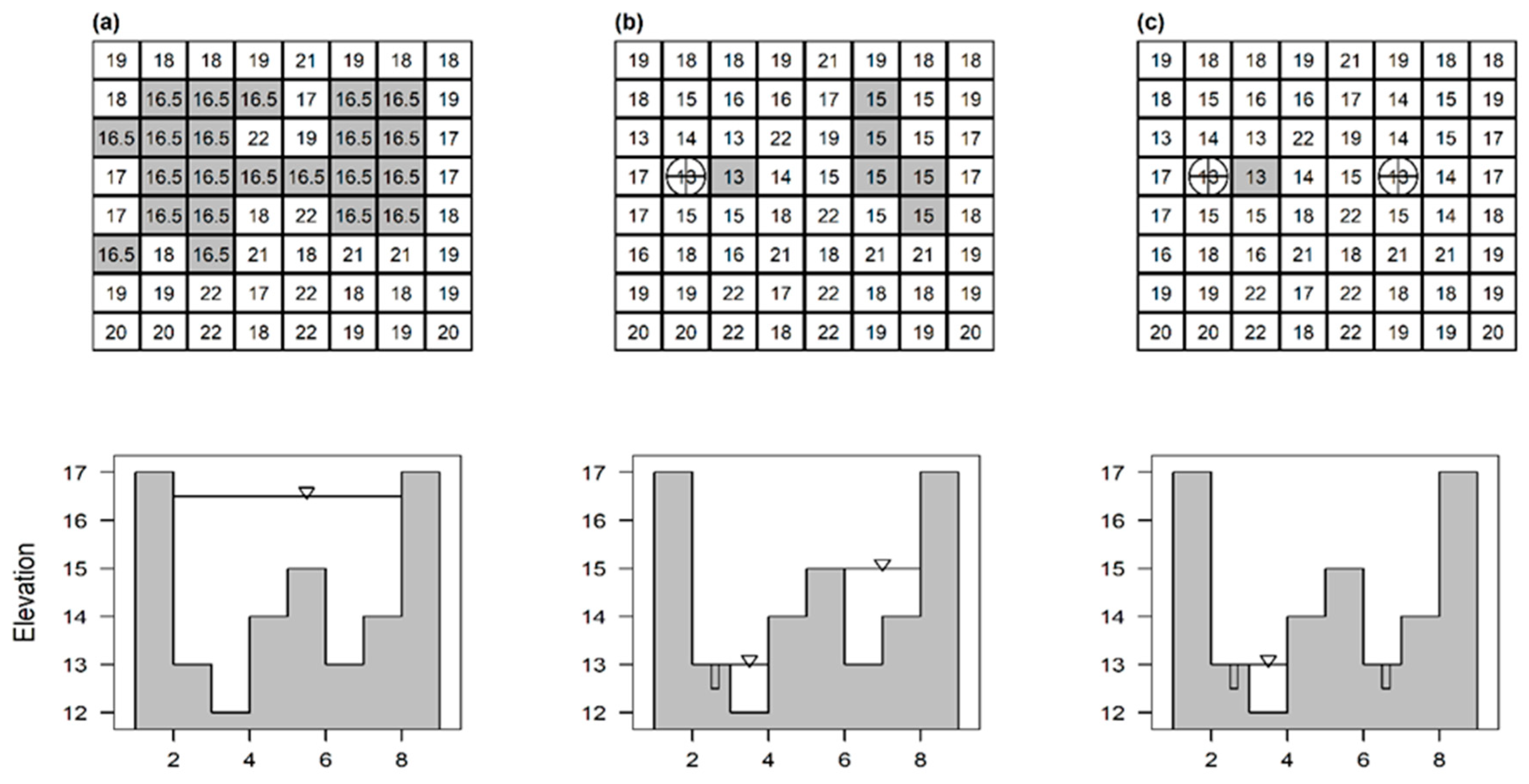
The flood recession module uses the location of manholes, the areal extent of the flood, as well as topography of the region to determine the aftermath of the flooded area. The flood recession method assumes that all flooded cells drain back to the manholes if there exists a flow path connecting them to the manholes; otherwise, it will remain ponded. Some of the flooded water in the local depressions can be disconnected from the manhole and will not fully be drained. Otherwise, the ponded locations can be distant from the manholes due to the topographic barrier.
2.2.1. Manhole Overland Flow Inundation Modeling
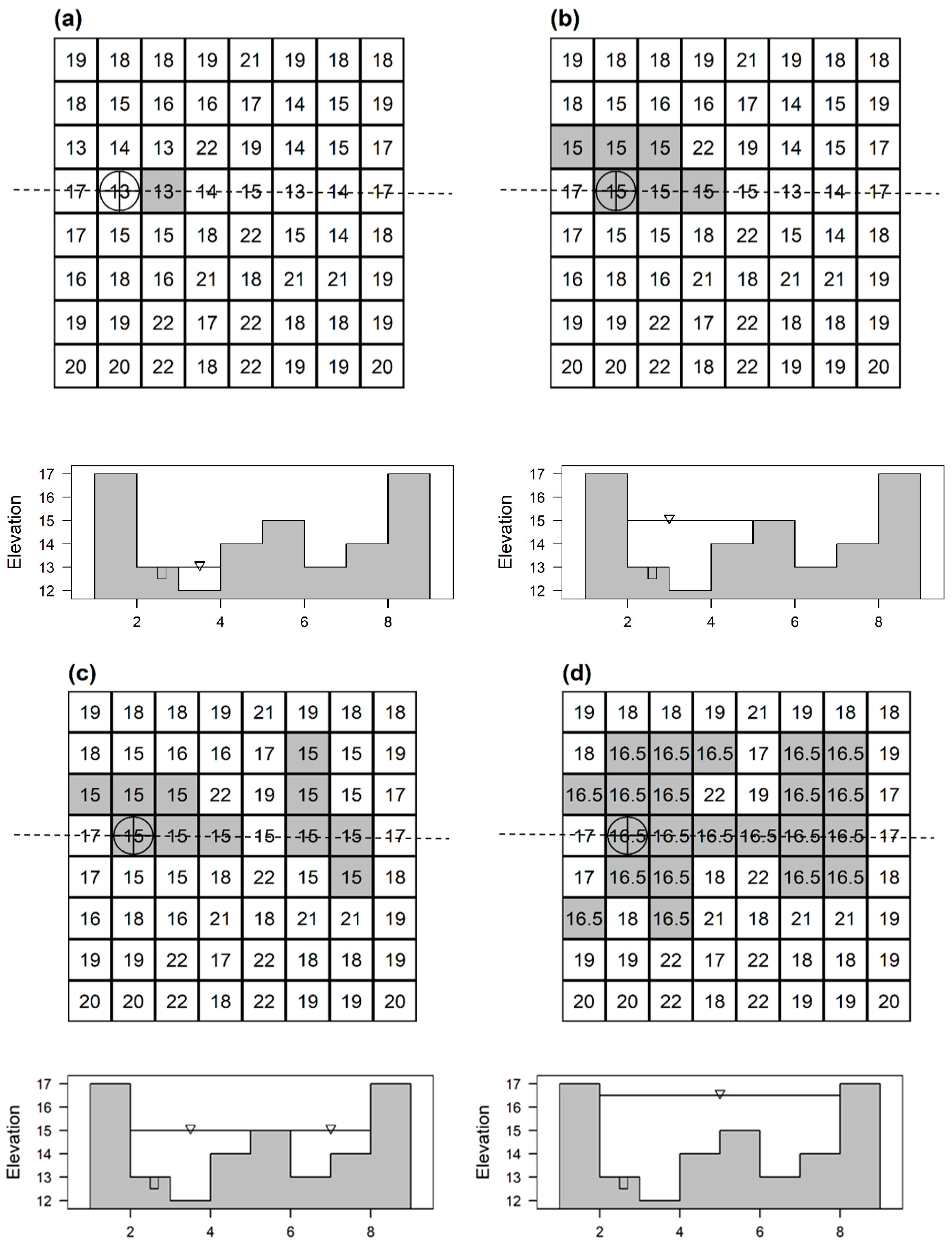
Our simulation of flood inundation is based on the elevation variations in neighboring cells. Starting from the cells containing the flooded manhole, floodwaters propagate to neighboring cells if the cell elevation is lower-than and connected-to a flooded cell. We used the D8 neighboring algorithm, which evaluates the elevations of the eight adjacent neighboring cells to each flooded cell, to determine the preferred flow direction (Figure 1). The flooded cells will maintain level flood surface and expand spatially as the lowest elevations are filled with available excess water. For multiple manholes overland flow, iterations are used to distribute all the overflows by maintaining the level flooded surface.
Before the flooding starts, the area is assumed dry, or the flood depths at each grid cell are known. Once the manhole overflow starts, the floodwater inundates neighboring and connected grid cells that have lower elevations (Figure 1). This inundation process will stop when the excess overland flow is completely allocated, and no water left to inundate the next dry cell. The flood inundation calculation is performed based on three main cases. In the first case, if the manhole cell elevation is smaller than that of the neighboring cells, the overflow will accumulate in the manhole cell until it reaches the minimum elevation of the neighboring grid cell. Once the overflow surface elevation exceeds the minimum elevation of a neighboring cell, the water will propagate spatially as long as there is enough overflow. In the second case, if the elevation of the manhole is higher than the elevations of neighbor cells, the overflow will be allocated automatically to the neighboring cells regardless of their slopes but maintaining level flooded surface. In the third case, if the elevation of the manhole is the same as the elevation of any neighboring cell, the excess water will be distributed equally among cells with the same elevations.
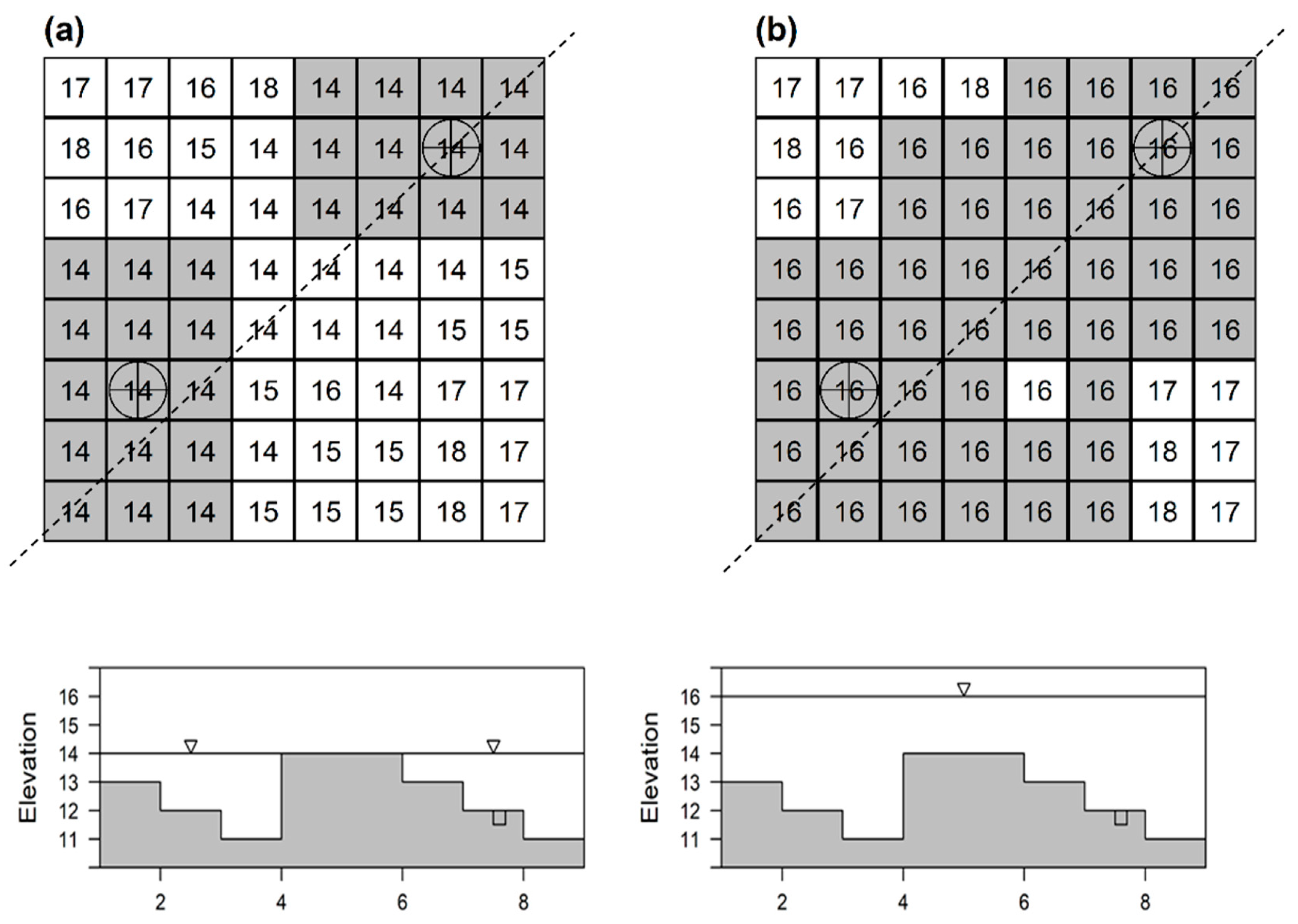
Figure 1 and Figure 2 show a schematic representation of flood inundations caused by overflow from one manhole and two manholes respectively. When the flood surface (surface elevation plus inundation depth) exceeds the elevation of the surrounding cells, the water will start to flow to the cells with the lowest elevations. As the overland flow increases, the neighboring cells will be gradually flooded while maintaining level flood surface. For example, when the overland volume is 49 units (Figure 1d), the extent of the flood coverage is first determined, based on the amount of the overland flow and elevation, and then the floodwater is distributed iteratively among the grids within the flooded area to maintain level flood surface. This iterative process considers the available flood volume, and recursively fills the next small neighboring cells.
Not explicitly considering the slope and land covers are the main limitation of the presented flood inundation approach. Similar to other grid-based hydrological and hydraulic modeling, the DSM resolution poses a high level of uncertainty in the model representation. Thus, the use of fine-resolution DSM and surface maps are critical for estimating the floods from manholes accurately [37]. For this study, we have used a one-meter resolution Light Detection and Ranging (LiDAR) DSM obtained from Washington State Department of Natural Resources. The model and the test cases do not include manhole inundation caused my previous storm and overland flow the drainage. Thus, we assumed dry terrain prior to the overflow from the manholes. However, in most cases, as the reviewer correctly stated, the manholes and their surrounding areas might already be flooded before the overflow. One simple modification is to adjust the terrain elevations for the inundation depth and then simulate the manhole overflow on top. Such an approach may work if the inundations surrounding the manholes that resulted from the previous storm were stationary, and have known flood depths. However, in most cases, the overland and overflow inundations from the drainage area and manholes, respectively, happen simultaneously, requiring a coupled simulation of both inundations.
2.2.2. Recession Modeling Associated with Manholes
Similar to the overland flow inundation, the flood recession to a given manhole considers the elevations of the surrounding grid cells and their connectivity to the manhole. For any given cell, the flooded water above the elevations of the adjacent grid cells will drain to the manhole if a flow path exists. Otherwise, it will remain ponded in the depressions. For example, when a manhole elevation is higher than the neighboring cells, only partial recession will occur. Starting from the manhole cell and expanding outward using the D8 algorithm, the recession model identifies flooded cells and drain them completely if their elevations are above one of the eight neighboring cells. Else drains part of the flooded water above the minimum elevation of the eight neighboring cells. As the grid cell expand spatially by searching adjacent eight neighboring, the connectivity of the target cell and the neighbor is traced using a flow path algorithm. For each flooded cell, the flow path algorithm detects the presence of any possible flow path to the manhole.
Figure 3 shows examples of flood recession based on single and multiple manholes. The result from the flood inundation estimate is given in Figure 3a. It is assumed that when rainfall ceased, the holding capacity of the drainage system decreases, and overland flow starts to recess toward the manholes. Figure 3b,c illustrate how flooded surfaces are recessing for a single and two manholes scenarios. The recession associated with a single manhole (Figure 3b) indicates two regions of ponding—one next to the manhole and another away from manhole caused by local topographic barrier. The ponded regions away from the manhole are not connected to the manhole hydraulically. The second case introduced an additional manhole in the depression region, and thereby the flood can be drained by the two independent manholes. The left manhole recess similarly as Figure 3b. The second manhole drains the ponded floodwater caused by a topographic barrier (Figure 3c).
2.3. Study Site: The Hall Creek Watershed
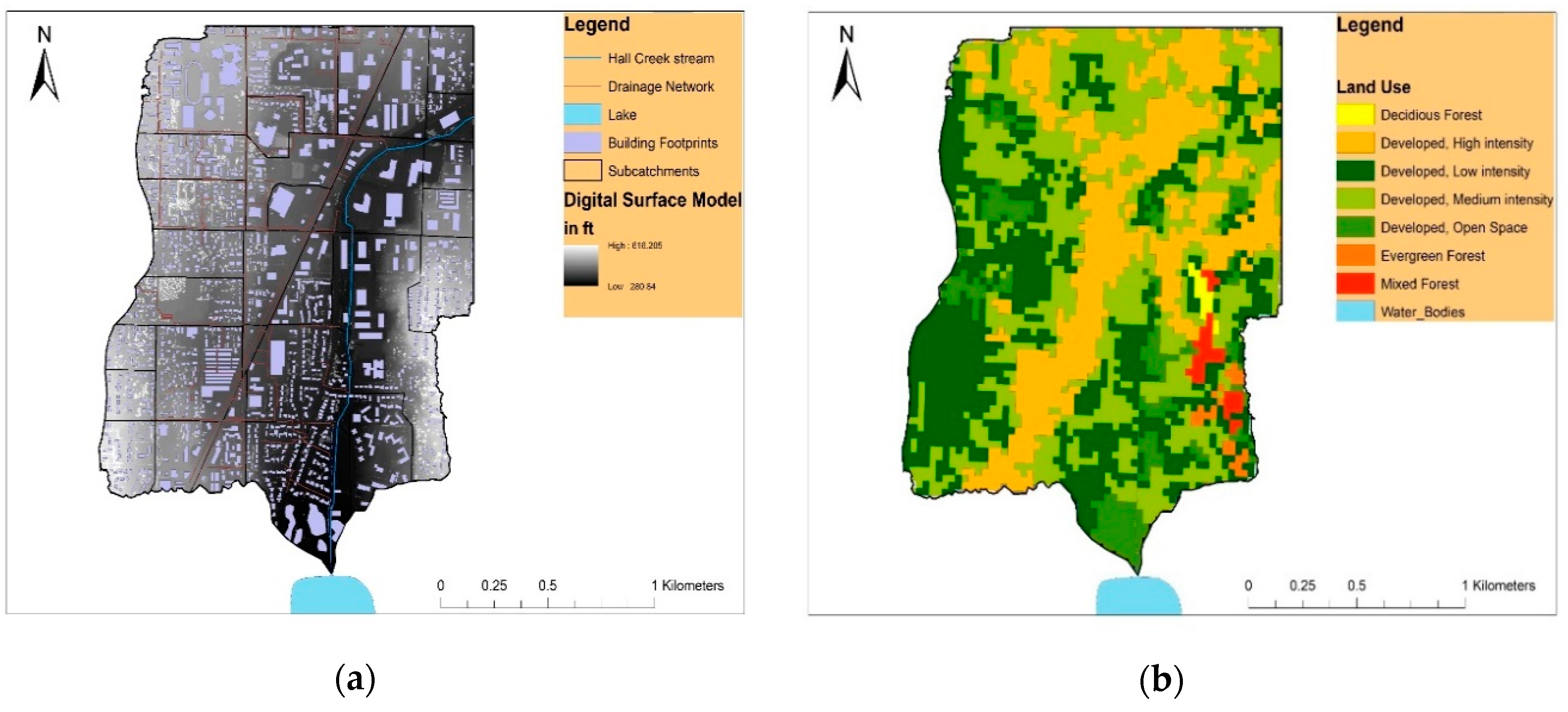
The Hall Creek watershed is an urban watershed (Figure 4), containing four major cities near Seattle, WA. These cities are Edmonds, Esperance, Lynnwood, and Mountlake Terrace, which are part of the northern Seattle–Tacoma–Bellevue metropolitan region. The predominant land cover type in the watershed is a developed urban region, which accounts for 96% of the land cover. The rest is covered by forest and water bodies (Figure 4b). The watershed is frequently affected by prolonged storm and flooding events.
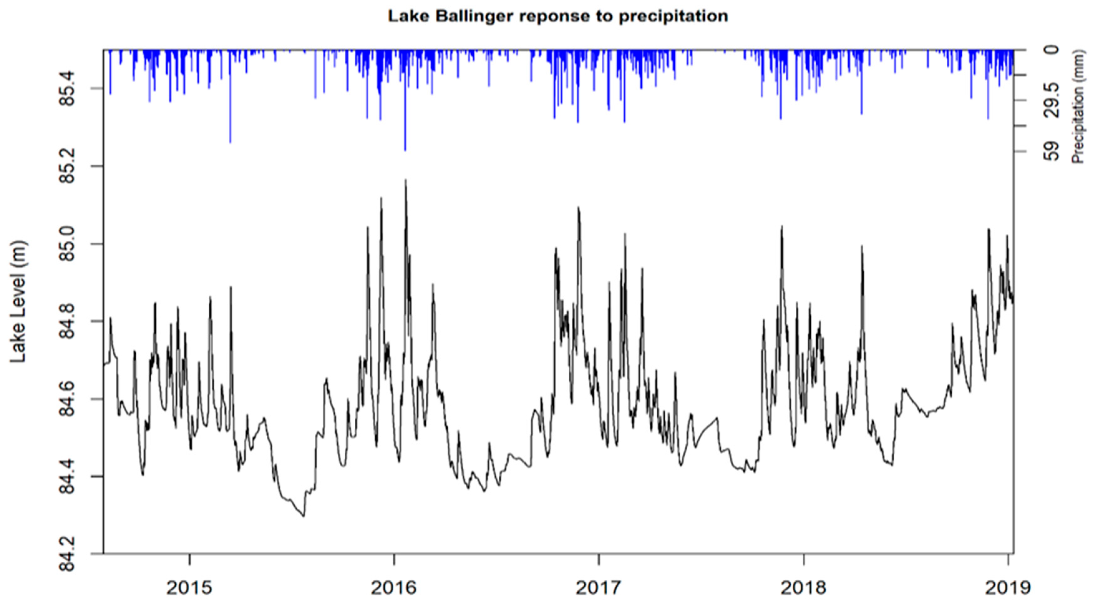
The Hall Creek is intermittent and drains toward Lake Ballinger. It is the main tributary to the Lake Ballinger [57,58], which discharges to the downstream McAleer Creek. The creek does not have a monitoring discharge and stage data. Since the lake level is highly influenced by storm events (Figure 5) and the flow from the Hall Creek, the available level data were used to calibrate the SWMM model.
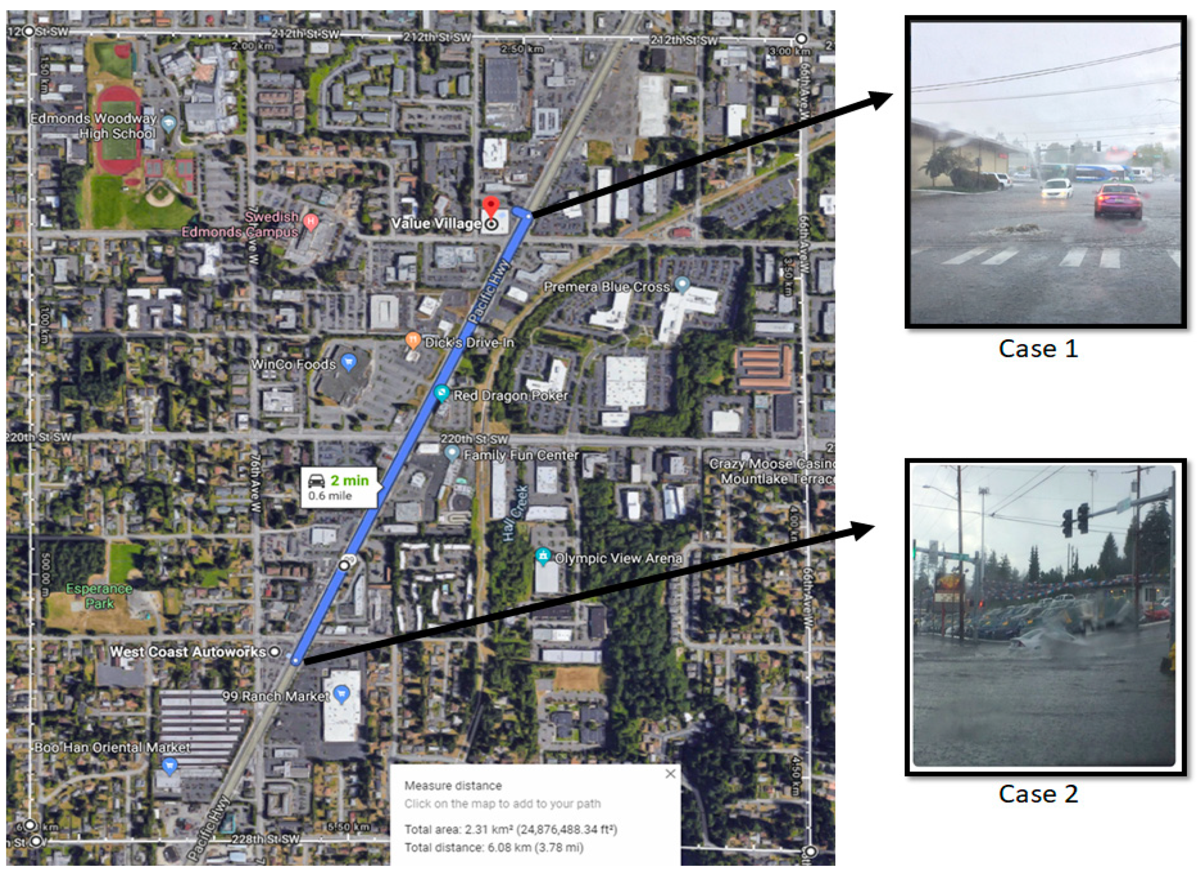
The flooding in the study area is mostly caused by storm events, while the urban area and street intersections are often affected by manhole overflow. For example, during the 19 September 2016 storm events, two manholes overflowed and caused flooding in the surrounding area. This flood event was used to validate our flood inundation and recession methodologies. One of the manholes flooded areas across a highway (Case 1), while the other caused flooding alongside the highway (Case 2) (Figure 6).
2.3.1. Data
High resolution observed meteorological data (obtained from the King County’s watersheds and rivers database) and sub-hourly lake level data (obtained from the city of Edmonds) were used to develop the SWMM model. Surface elevation from a one-meter resolution LiDAR data (obtained from Washington State Department of Natural Resources) were used for the flood inundation and recession modeling. We have extracted the conveyance network system of the city of Edmonds and Mountlake Terrace from their respective Geographical Information System (GIS) Department. We have identified the type, location, and possible flow direction of the sewer system. The land cover data were obtained from the US Department of Agriculture and were used to estimate the percentage of impervious layer. For the purpose of calibration and validation of the FIRM model, the observed flood boundaries are delineated using related images (Figure 6) and texts from social media users (such as locations). We used Google Earth and high-resolution LiDAR data to determine the relative topographical variation and delineated the inferred flood boundary by considering 360-street and panoramic view. We also used the city of Edmonds GIS-dataset to correlate the inferred flood boundary and building footprints to check if there exists a mismatch between the building blocks and the street boundaries.
2.3.2. SWMM Model
The SWMM model was discretized into 32 sub-catchments based on the hydrological and drainage network criteria. These criteria include percent of land cover, slope, availability of conveyance network system, and percent of impervious layers. A 5% of land use, slope, and soil type is used to subdivide the catchment. The sub-catchment layer, conduit layer and node layers are used for urban watershed discretization. After the watershed was discretized, the external inputs such as precipitation, temperature, and evapotranspiration were extracted and applied for each sub-catchment. The hydraulic properties of manholes, storage, ditches, culverts, and other structures were incorporated. There are total of 106 manholes, one storage, and 108 nodes connected by conduits in the study area. Only 40% of the manholes were considered in our study based on consideration of data availabilities and the computational requirement of the SWMM model. The Hall Creek flux are represented using SWMM’s inflow package. Despite the reasonable performance of our model in representing the hydrology and hydraulics of the study area (Section 3.1), not considering all the hydraulic structures in our model might have introduced some level of uncertainty that need for a further study. SWMM simulations can take hours if the model domain is large and accompanied by detailed complex hydraulic structures and sub-daily meteorological and hydrological input variables. The model simulation was conducted using the “swmmr” R-package [55].
Model calibration can be performed using either manual or automated method [59]. In this study, we used both methods of calibration to ensure usage of their advantages. First, we used manual calibration to identify sensitive parameters. The sensitive parameters was then further calibrated using differential evolution (DE) method, which finds the global optimum parameters values for continuous and differentiable functions [60], based on successive generation and transformation of the parameters values under a given fitness-measured criteria [53]. The DE requires defining parameters upper and lower bounds, objective function, and the lower or the upper optimal solution goal. The algorithm starts by randomly dividing the parameters values in to three distinct populations. The parameters values from each population are then combined to generate the next sets of populations that minimize the objective function. To ensure global optimal solution, the algorithm uses mutation to include non-optimal parameters values in the new populations [53]. The evolution continues until it meets the objective function criteria.
Due to the lack of discharge observational data for the Hall Creek, the model calibration and validation were performed based on the lake level fluctuation of Lake Ballinger, which is located at the outlet of the creek. Since the creek is a main feed to the lake, the lake level fluctuations reflect the changes in the creek discharge. The model calibration includes the initial condition of the model, which enables to determine the calibration parameter ranges, and optimization of the parameters using differential evolution optimized method [61]. Nearly three (2.7) years of data were used to calibrate the model, and one-year of data were used for validation.
The initialization was used to identify sensitive parameters and their respective parameter ranges. The model was then optimized using the differential evolution method, namely the “DEoptim” packages [61]. Differential Evolution (DE) is a genetic algorithm that finds global optimum values for continuous and differentiable functions [60] based on successive generation and transformation of the parameter sets [53]. The DE requires parameters for upper and lower bounds and an objective function for the optimization. During each evolution, in addition to identifying the better parameter sets (or population), the algorithm also introduces a random change to those parameter sets to ultimately get the global optimal parameter values.
The model simulation includes spin up, main (calibration), and post-audit (validation) simulations. Fitness measure statistics, including Nash–Sutcliffe efficiency (NSE), percent bias (PBIAS), root-mean-square error (RMSE), ratio of the RMSE to the standard deviation of measured data (RSR), and Kling–Gupta efficiency (KGE) were used to evaluate the model calibration results. The NSE compares the variance of the residuals (or fitting difference) with the variance of observed lake levels [62]. The PBIAS measures the average residuals or deviations of model results from observed lake levels [63]. The RMSE measures how spread out these residuals from the model results. The RSR is a normalized RMSE by the standard deviation of the observed lake level [64]. The KGE uses the idea of diagnostic decomposition, where the NSE is breakdown into three components (the relative importance of correlation, bias, and variance difference) [63,65]. The KGE ranges from negative infinity to one, with the optimal model prediction having the KGE value close to one.
Where Yobs is observed, Ysim is simulated, Ymean is the mean of the observed lake level change, r is correlation coefficient between the modeled and observed lake levels; γ is a ratio between the standard deviation of modeled and observed lake levels and β is a ratio between the standard deviation and mean of the modeled and observed lake levels (Table 1).
Manhole overflows were extracted from the calibrated SWMM model and were used as input for the FIRM simulation. The spatial extent of the model is compared to the observed flood regions. Since there was no direct measurement of flood spatial extent and depth, the observed flood area was reconstructed based on pictures of the area taken during the flood event and obtained from social media twitter. The social media information includes both pictures, texts, and street names, allowing us to identify the exact locations and extent of the flood. The previous reports in the cities also indicated that there had been multiple incidences of pluvial flooding near side roads and along intersections. This information was used to delineate the observed flood region, which was then used to validate the flood inundation model. The process of flood boundary delineation is depicted, in Figure 6, which show how the flooded region in the study area was extracted from social media outlets. The images and the text by users are used to identify the exact location of the flooded regions. We used google-earth and high-resolution LiDAR data to determine the relative topographical variation and delineated the inferred flood boundary by considering 360-street and panoramic view. We also used the city of Edmonds GIS-dataset to correlate the inferred flood boundary and building footprints to check if there exist mismatch between the ground and the street boundaries.
2.4. Model Inundation Accuracy
The model’s ability to detect the spatial accuracy of the flood extent was evaluated based on the true positive rate (TPR), the positive predictive value (PPV), the modified fit (MF), and the modified bias (MB) methods. The TPR and PPV are derived from the confusion matrix [17], which is a 2-by−2 matrix containing the TPR and PPV for gridded simulated and observed flood conditions (Table 2). These statistics were used recently to assess the flood inundation model performance in [39,66,67]. TPR measures how well the modeled flood region replicates the observed flood boundary. The maximum TPR (100%) represents that the model fully captures the observed flooded regions. The TPR indicates the model tendency to under-predict the flood hazard [39,66,67]. PPV measures how well the model captures flooded in the model but dry in observation. The value ranges from 0%, indicating over prediction of the flood extent, to 100% for accurately captured the observed boundary.
Flood inundation and recession model (FIRM); true positive rate (TPR); the positive predictive value (PPV); true positive (TP); false negative (FN); false positive (FP); true negative (TN).
Where TP represents the flooded regions in both the observation and model simulation, FP represents the flooded region in the model but dry in the observation, and FN represents regions flooded in reality (i.e., in observation) but simulated as dry. The TPR and PPV percentages represent the overlapping rate between simulated and observed flood areas. Higher percentage values of TPR and PPV indicate higher accuracy of the flood inundation model. The two statistics must be used in combination to measure the accuracy of the model since they each evaluate the different performance of the model. Specifically, the TPR and PPV measure how well the model captures the observed flood and flooded pixel that are dry in observation, respectively. For example, the TRP value can be 100% if the model captures all the observed flooded cells even though it may also consider some dry cells as flooded (refer to Equation (3)). Similarly, the PPV value can be 100% if the model captures all the dry cell even though it may also consider some flooded cell as dry.
Other methods of model performance evaluation are fit and bias indicators, which are also commonly used for flood inundation modeling [40,44,68,69,70]. Previous studies used both fit and bias indicators to compare flood inundation extents between different models. For this research, we infer observed flood extents based on street photos taken during the actual flood event and compare them with the flood inundation results from our model. The modified fit indicator is calculated based on overlapping areas between observed and simulated inundated areas. The indicator ranges from 0% to 100% for poor and ideal model performances, respectively. While the modified bias indicates the overall difference between the simulated and observed flood extents. Positive and negative modified biases indicate an overestimation and underestimation of flood extents by the model, respectively.
3. Results and Discussion
3.1. SWMM Model Calibration and Validation
We compared simulated versus observed lake level changes, and show our model captures the lake level fluctuations reasonably well (Figure 7, Figure 8 and Figure 9). The main objective of the SWMM simulation was to estimate the flood condition in Edmonds from the 19 September, 2016 storm event. For model stability and to represent preexisting hydrological conditions such as soil moisture content, we considered ten months (from 1 August, 2015 to 31 May 2016) of simulation as a spin up. The model calibrated using data from 1 June 2015 to 31 January 2018; and validated using data from 1 February, 2018 to 10 January 2019. After the sensitivity analysis using the manual calibration, we identified five parameters for model calibration. These includes the imperviousness percentage, width, roughness coefficient, depression storage, and the hydraulic conductivity of the soil. The calibration is performed in the DEoptim R-package. Table 3 indicates the upper and lower limits of the model parameters used in the calibration process.
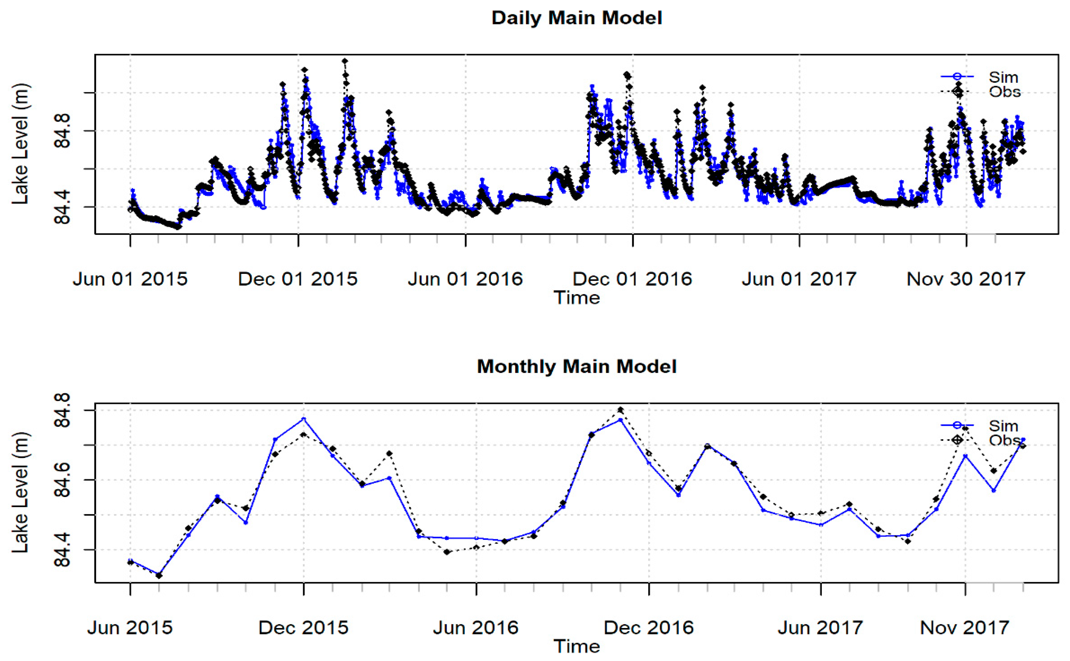
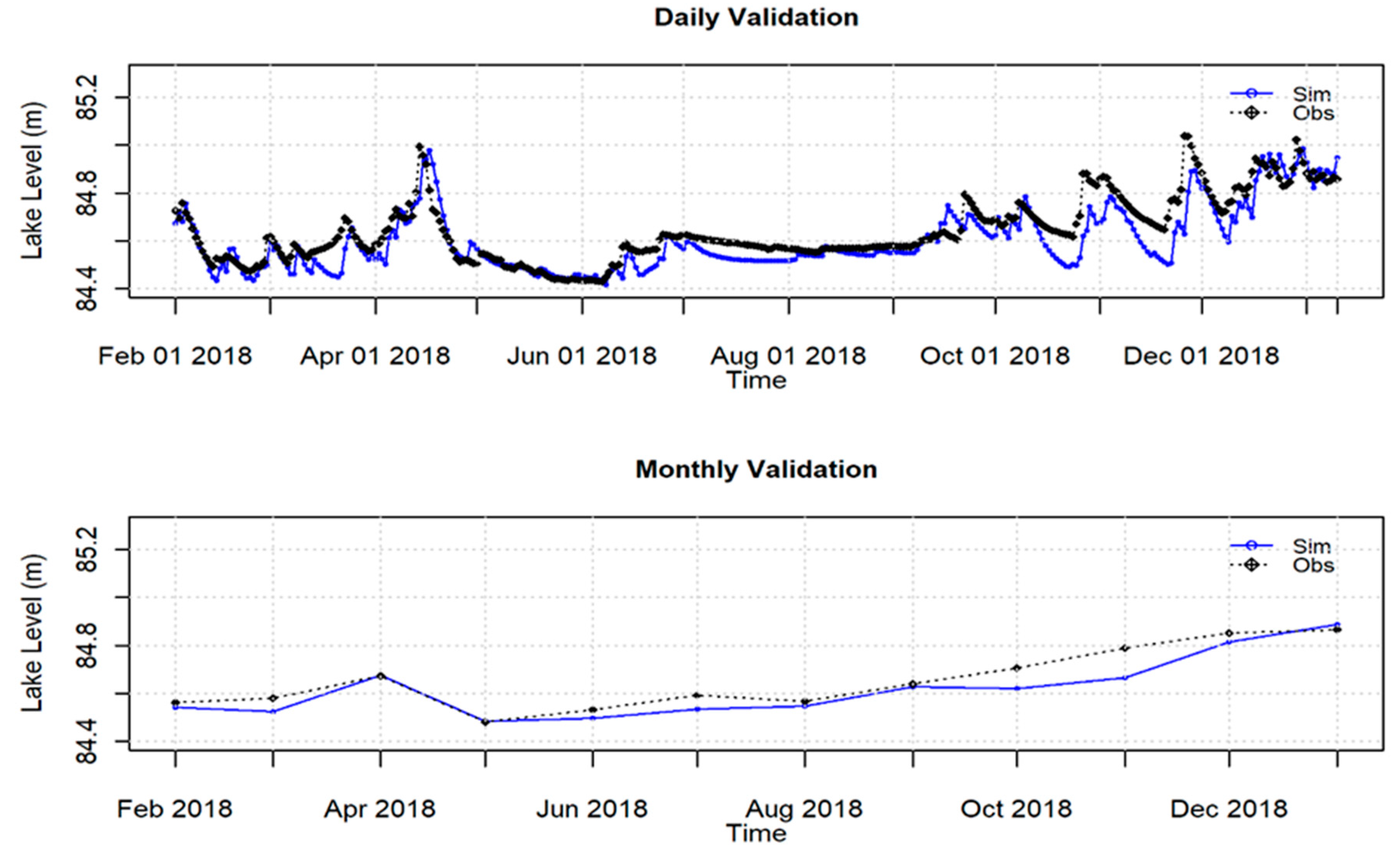
Figure 7 and Figure 8 shows the comparison of the model simulation and observed time series plots for daily and monthly average lake level change for the calibration and validation simulation periods, respectively. The figures demonstrate that the lake level changes as a result of storm events were reasonably captured for the calibration period. The validation results for both daily and monthly observed and simulated lake levels show the ability of the model to predict beyond the calibration period.
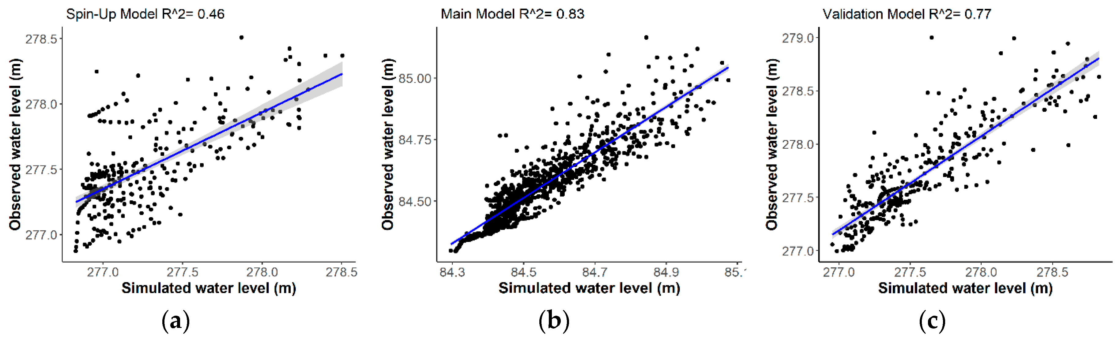
Figure 9 indicates the correlation between the observed and simulated lake level change for spin-up, the main model simulation, and the validation period. The regression coefficient (R2) is 0.42 for the spin up period, 0.83 for the calibration period, and 0.77 for the validation model simulation period. The correlation coefficients for the calibration and validation period also confirm the model captured the observed lake level reasonably well. The simulation was also evaluated using the NSE, KGE, RSR, and PBIAS.
The statistical summary of the spin up, calibration and validation simulations results are presented in Table 4. For the calibration and validation periods, the KGE are 0.91 and 0.88, respectively, while the NSE is 0.82 and 0.67. These indicate satisfactory model performance. The RSR, which indicates the variation in the residuals, is between 0 and 0.5. This is considered a very good performance [71]. The PBIAS values are also close to 0, which confirm that the model simulates the observed water level with minimal bias. Compared to the daily model performance, the monthly model performance is improved.
3.2. Flood Inundation and Recession
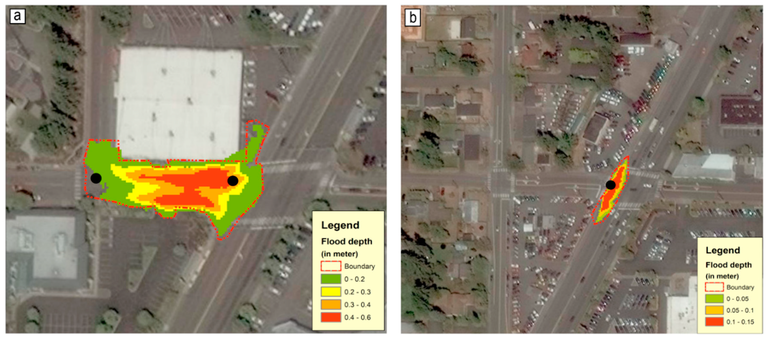
The spatial extent and depth of the flood inundation were simulated for a pluvial flood event that happened on 19 September 2016 using FIRM. A detailed conveyance network system with sub-daily meteorological data, such as rainfall data, were used to capture the flood event using SWMM continuous simulation. The FIRM simulate the floods caused by overflow from two manholes, and its results were compared with the inferred flood boundary (Figure 10). Figure 10 represents the areal extent and depth of the flood inundation at two locations. The red dot-line represents the inferred flood boundary, and the black point represents manholes. The color represents flooding depth. The fine-resolution LiDAR data were able to identify detailed urban infrastructures, such as building food prints, and streets. The FIRM was able to identify elevated urban infrastructures and with low-lying streets. Overall, coupling both the 1D SWMM model with the 2D FIRM model was able to delineate the spatial extent and depth of the flood generated from manholes overflow in the study area.
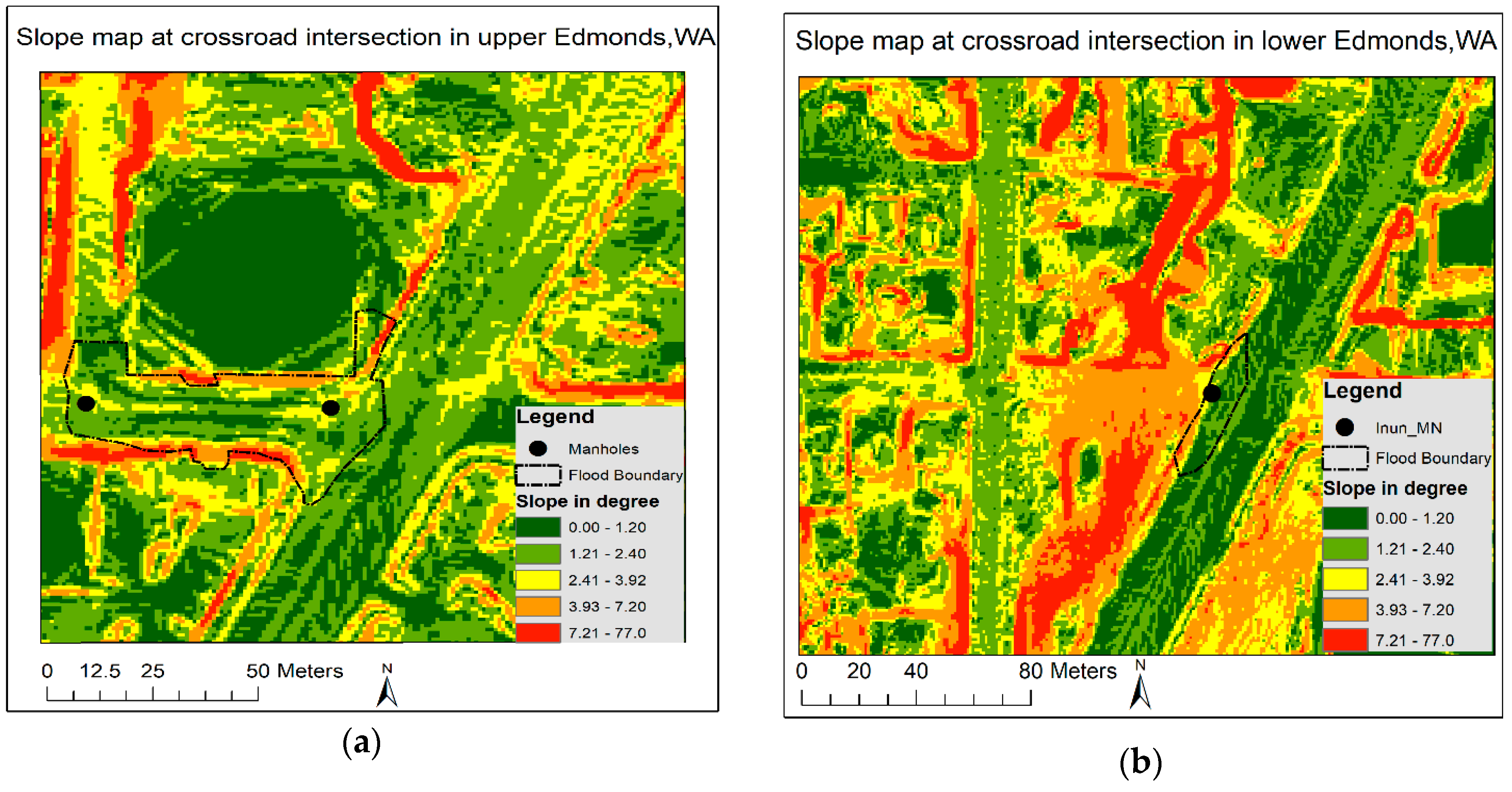
The flood started from a given manhole and propagated spatially by filling any neighboring grid cells with lower elevations. As shown in Figure 10a, representing Case 1, the flood is concentrated across a highway going west to east. The topographic variations around the manhole are relatively small, with the mean slope of the flooded region being 1.2 degrees (Figure 11a). The flat slope, particularly along the street, enables the overland flow to inundate along the street perpendicular to the main highway. Based on the FIRM result, the areal extent, maximum flood depth and volume of the inundation region is 2129 m2, 0.6 m, and 710 m3, respectively. The depth of the flood is controlled by the local elevation and the amount of the excess overland flow. The low-lying part of the street generally has deeper flood depth compared to the peripheral part of the flood extent. Hence, the pavement is often elevated compared with the street elevation. Another manhole flooding in our study (Figure 10b, Case 2) was used to evaluate the flood inundation simulation. In this case, the manhole is located in the steeper part of the street, where the average slope of the street is 5.2 degrees from the west to east (Figure 11b). Consequently, the flood is mostly concentrated along with the highway in the north and south direction, and did not spread much laterally. The volume, areal extent, and maximum depth of the flooded region are 38 m3, 426 m2, and 0.15 m, respectively.
Based on the two cases, we observe that the flood inundation model considers the spatial heterogeneity of the surface feature to inundate, for example, flood inundation algorithm was able to differentiate building with streets (Figure 10a) and intersections of streets with varying slope and elevation (Figure 10b). FIRM inundates the lowest level and cover wider area for a relatively gentle region. Conversely, for the manhole located in a steeper region, the algorithm follows the preferred flow direction and inundate relatively smaller area.
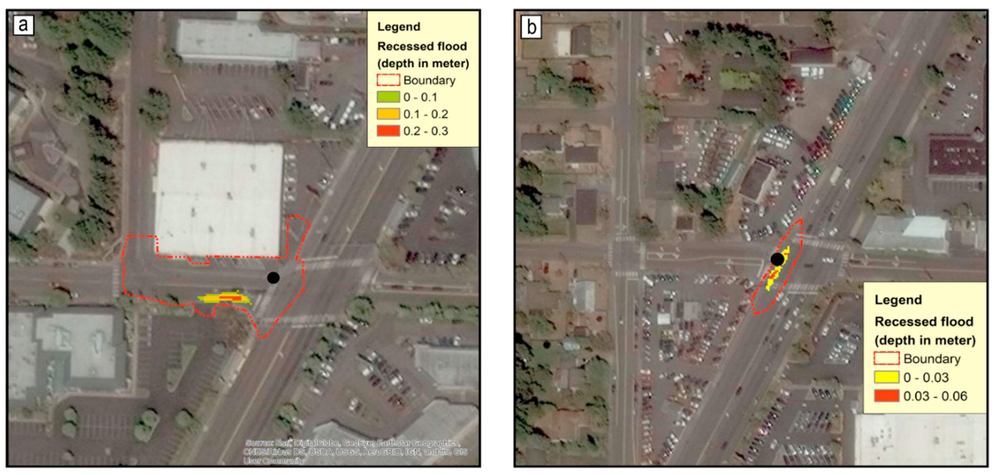
To determine the flood recession, we assumed that once the storm ceased and the pipe full capacity decreased, the water eventually drains back to the conveyance system unless it is isolated from the manhole because of depression storages. Accordingly, some of the inundated floodwaters may recess, while the remaining waters are left as ponding associated with local topographic barriers. The result for Case 1 shows that most of the floodwaters drain since the manhole is located at a lower elevation. There is some ponded water away from the manhole due to possible topographic barriers between the manhole and the flooded areas (Figure 12a). Since the manhole is located at a lower elevation, most of the flooded water drained to the manhole. The volume, areal extent, and maximum depth of the ponded region are 15 m3, 89 m2, and 0.17 m, respectively. For Case 2, the ponded water is generally concentrated near the manhole due to the local topographical depression around the manhole (Figure 12b). The flood volume, the areal and depth of the ponded water decreases to 3 m3, 85 m2, and 0.06 m, respectively. The results showed the FIRM abilities to determine the maximum flood extent and the extent aftermath of a given storm. Each information is important to assess the flooding risk and associated potential short-term (flood inundation) and long-term (flood recession) impacts.
3.3. Model Inundation and Recession Accuracy
In addition to the visual comparison of the observed and simulated flood areas, the model performance evaluation for the inundation was carried out using statistical measures that compare the simulated and observed gridded flood areas. This enables us to identify and assess the model performance based on how accurately the model predicted the observed flooded and dry regions. We adopted the TPR and PPV from [66] and used the modified version of the fitting (MF) and bias (MB) indicators from [44,70]. The model inundation extents are compared with the inferred observed flood boundaries that were extracted from photos of the flood boundaries.
Table 5 shows the model performance indicators used to evaluate the flood inundation model based on the inferred flood regions. The TPR for Case 1 (89%) indicates the model’s ability to capture the flooded grid cells, while for Case 2, the TRP is 71%, indicating the model predicted a relatively more flooded region as dry land. Thus, the model under predict the flood hazard in Case 2. The PPV for Case 1 and Case 2 are found to be 95.4% and 97.25%, respectively. These indicate the model’s ability to capture the observed none flooded cells. The MF of 85% for Case 1 indicates that the model has better agreements with the observed flood boundary compared to that of Case 2, which has MF of 69.90%, indicating the existence of relatively large variation between the predicted and observed flooded regions. The negative values of the MB for both cases indicates that the flooded regions in both cases were underestimated. Overall, the relative errors are relatively higher for Case 2 compared to Case 1. This is due to underestimating the flood hazard in Case 2 compare with the observed boundary, and possibly due lack of the FIRM to simulate the impact of direct rainfall during the flood events or lack to represent flood water loses into the buildings.
The low TPR values compared to the PPV values suggest that the flood inundation model underestimated the total flooded regions for both cases; but predicted well the flooded region within the observed flood boundaries (Figure 10). The underestimation of the flood areas might be due to the model inundation algorithm not incorporating the additional flooding resulted from direct precipitation or generated surface runoff. The relatively poor performance of the model for Case 2 might also be due to the inundation algorithm limitation to incorporate direct additional flood flux from upstream overland flow into the flooded regions. In addition, the relatively higher slopes in the area, which facilities rapid overland flow from the manhole toward the low elevated regions, may have impacted the model performance. Moreover, the relatively better model performance for Case 1 might be because of the relatively homogenous topography in the area, which is well represented by the 1-m LiDAR data.
Coupling the FIRM model and hydrodynamic model with projected future storm scenarios may help to identify areas that may experience future manhole flooding. This modeling capability can help to better assess flooding risk, and improve designs of storm water drainage systems in flood-prone urban areas. To further improve the work, it is important to consider direct rainfall during storm events and other sources or losses of floodwaters (e.g., possible loses of floodwater by draining into the building or addition of excess runoff from rooftops), as well as the land cover and slopes.
4. Conclusions
We have presented effective flood inundation and recession methodologies that use overflow from given manholes and topography of an urban region. We used the SWWM model to estimate the volume of overflow from manholes. In order to determine the associated flood depth and extent during and after storm events, we developed a flood inundation and recession model (FIRM) that uses high-resolution LIDAR elevation data. SWMM was developed on the basis of watershed characteristics and the drainage conveyance network in the area. SWMM was calibrated using a differential evolution optimization method and validated based on observed lake level data at the outlet of the watershed. The manhole overflows were extracted and used in FIRM to delineate the spatial extent and flood depths.
The spatial extent of the simulated flood area was compared with the observed flood boundary, which was derived from social media pictures and reports from the cities. Two case studies, based on flood events in Edmonds, WA, were considered to evaluate the flood inundation and recession model. In these case studies, the flood occurred across and along a main highway under different topographical characteristics. The results showed that the spatial extent of the flood regions is highly influenced by local topography and the position of the manholes. Particularly, the spatial arrangement of the manhole and the slope of nearby areas are crucial for determining the spatial extent, spatial heterogeneity of the flood depth, and selecting preferential flow paths to inundate low-lying areas. The model is able to capture the flood extent for manhole overland flow in fluvial flood events. Incorporating the direct impact of rainfall on the fluvial flood event can improve the representation of the physical process and the accuracy of the model. As the flood recession observation data are scarce, the performance of the flood recession model result was difficult to quantify. Finally, proper understanding and representation of the study area, the boundary condition, and engineering structures are important for the flood inundation and recession modeling associated with manhole overland flow.
Regional authorities can utilize the presented model (FIRM) by coupling with existing hydrodynamic modeling (e.g., SWMM) to quantify flood hazard based on pluvial generated overland flooding and manholes induced flooding in urban areas, where flood mechanism is complex and modified by local infrastructures. FIRM can be used to estimate the areal extent and depth of flood caused by manholes overland flow during a flood event (flood inundation) and after the event is over (flood recession). Because of the relative simplicity of the model and its uses of readily available data, the model can be used for a real-time assessment of flood progression and to identify potential impact areas. The model’s ability to simulate flood recession will also allow identifying areas where the flooded water will remain ponded for days after the floodwater subsides. The ponded water, or the floodwater not drained, can impact human health and properties. In addition to the real-time forecast of flood inundation and estimation of the aftermath ponding condition for the existing drainage system, the model can be used to design better a new or retrofit the current drainage system to minimize the overflow and ponding after the flood events. The model can be used to assess the flood condition under multiple storms, watershed conditions, and drainage scenarios. It can contribute to our understanding of climate change and appropriate engineering designs for mitigation.
Author Contributions
Conceptualization, M.G. and Y.D.; methodology, M.G. and Y.D.; validation, M.G. and Y.D.; writing—original draft preparation, M.G.; writing—review and editing, M.G. and Y.D.; supervision, Y.D.; funding acquisition, Y.D. All authors have read and agreed to the published version of the manuscript.
Funding
Department of Defense’s Strategic Environmental Research and Development Program (SERDP) under contract W912HQ-15-C-0023.
Acknowledgments
We are thankful for the city of Edmonds and Mountlake Terrace for providing sewer network dataset and observation data. The first author is grateful for the research input from Joan Wu, Akram Hossain, Jennifer Adam, Mark Wigmosta, Debra Perrone, and Scott Jasechko. We are thankful for the anonymous reviewers for helpful comments on the manuscript.
Conflicts of Interest
The authors declare no conflict of interest. The funders had no role in the design of the study; in the collection, analyses, or interpretation of data; in the writing of the manuscript, or in the decision to publish the results.
References
- Wallemacq, P.; Herden, C.; House, R. The Human Cost of Natural Disasters 2015: A Global Perspective; Technical report; Centre for Research on the Epidemiology of Disasters: Brussels, Belgium, 2015. [Google Scholar]
- Stocker, T.F.; Qin, D.; Plattner, G.-K.; Tignor, M.; Allen, S.K.; Boschung, J.; Nauels, A.; Xia, Y.; Bex, V.; Midgley, P.M. Climate change 2013: The physical science basis. In Contribution of Working Group I to the Fifth Assessment Report of the Intergovernmental Panel on Climate Change; Cambridge University Press: Cambridge, UK, 2013; Volume 1535. [Google Scholar]
- Technical Mapping Advisory Council (TMAC). Technical Mapping Advisory Council (TMAC) 2015 Annual Report Summary. Available online: https://www.fema.gov/media-library-data/1454954186441-34ff688ee1abc00873df80c4d323a4df/TMAC_2015_Annual_Report_Summary.pdf (accessed on 13 March 2020).
- Federal Emergency Management Agency (FEMA). Loss Dollars Paid by Calendar Year. Available online: https://www.fema.gov/loss-dollars-paid-calendar-year (accessed on 13 March 2020).
- European Environmental Agency (EEA). Mapping the impacts of natural hazards and technological accidents in Europe – an overview of the last decade. EEA Technical Report No13/2010. Available online: https://www.eea.europa.eu/publications/mapping-the-impacts-of-natural (accessed on 13 March 2020).
- Wang, W.; Li, H.Y.; Leung, L.R.; Yigzaw, W.; Zhao, J.; Lu, H.; Deng, Z.; Demisie, Y.; Blöschl, G. Nonlinear filtering effects of reservoirs on flood frequency curves at the regional scale. Water Resour. Res. 2017, 53, 8277–8292. [Google Scholar] [CrossRef]
- Ye, S.; Li, H.-Y.; Leung, L.R.; Guo, J.; Ran, Q.; Demissie, Y.; Sivapalan, M. Understanding flood seasonality and its temporal shifts within the contiguous United States. J. Hydrometeorol. 2017, 18, 1997–2009. [Google Scholar] [CrossRef]
- Milner, A.M.; Picken, J.L.; Klaar, M.J.; Robertson, A.L.; Clitherow, L.R.; Eagle, L.; Brown, L.E. River ecosystem resilience to extreme flood events. Ecol. Evol. 2018, 8, 8354–8363. [Google Scholar] [CrossRef] [PubMed] [Green Version]
- Scanlon, B.R.; Keese, K.E.; Flint, A.L.; Flint, L.E.; Gaye, C.B.; Edmunds, W.M.; Simmers, I. Global synthesis of groundwater recharge in semiarid and arid regions. Hydrol. Processes 2006, 20, 3335–3370. [Google Scholar] [CrossRef]
- Wang, X.; Zhang, G.; Xu, Y.J. Impacts of the 2013 extreme flood in Northeast China on regional groundwater depth and quality. Water 2015, 7, 4575–4592. [Google Scholar] [CrossRef] [Green Version]
- Jasechko, S.; Birks, S.J.; Gleeson, T.; Wada, Y.; Fawcett, P.J.; Sharp, Z.D.; McDonnell, J.J.; Welker, J.M. The pronounced seasonality of global groundwater recharge. Water Resour. Res. 2014, 50, 8845–8867. [Google Scholar] [CrossRef] [Green Version]
- Cuthbert, M.O.; Taylor, R.G.; Favreau, G.; Todd, M.C.; Shamsudduha, M.; Villholth, K.G.; MacDonald, A.M.; Scanlon, B.R.; Kotchoni, D.V.; Vouillamoz, J.-M. Observed controls on resilience of groundwater to climate variability in sub-Saharan Africa. Nature 2019, 572, 230–234. [Google Scholar] [CrossRef]
- Dahlke, H.; Brown, A.; Orloff, S.; Putnam, D.; O’Geen, T. Managed winter flooding of alfalfa recharges groundwater with minimal crop damage. Calif. Agr. 2018, 72, 65–75. [Google Scholar] [CrossRef] [Green Version]
- GebreEgziabher, M. An Integrated Hydrogeological Study to Understand the Groundwater Flow Dynamics in Raya Valley Basin, Northern Ethiopia: Hydrochemistry, Isotope Hydrology and Flow Modeling Approaches. Master’s Thesis, Addis Ababa University, Addis Ababa, Ethiopia, 2011. [Google Scholar]
- Changnon, S.A., Jr. Recent studies of urban effects on precipitation in the United States. Bull. Am. Meteorol. Soc. 1969, 50, 411–421. [Google Scholar] [CrossRef]
- Arnbjerg-Nielsen, K.; Willems, P.; Olsson, J.; Beecham, S.; Pathirana, A.; Bülow Gregersen, I.; Madsen, H.; Nguyen, V.-T.-V. Impacts of climate change on rainfall extremes and urban drainage systems: A review. Water Sci. Technol. 2013, 68, 16–28. [Google Scholar] [CrossRef]
- Boyd, E.; Juhola, S. Adaptive climate change governance for urban resilience. Urban Stud. 2015, 52, 1234–1264. [Google Scholar] [CrossRef]
- Ford, A.; Barr, S.; Dawson, R.; Virgo, J.; Batty, M.; Hall, J. A multi-scale urban integrated assessment framework for climate change studies: A flooding application. Comput. Environ. Urban 2019, 75, 229–243. [Google Scholar] [CrossRef]
- Chen, J.; Hill, A.A.; Urbano, L.D. A GIS-based model for urban flood inundation. J. Hydrol. 2009, 373, 184–192. [Google Scholar] [CrossRef]
- Wang, R.-Q.; Mao, H.; Wang, Y.; Rae, C.; Shaw, W. Hyper-resolution monitoring of urban flooding with social media and crowdsourcing data. Comput. Geosci. 2018, 111, 139–147. [Google Scholar] [CrossRef] [Green Version]
- National Academies of Sciences, Engineering, and Medicine. Framing the Challenge of Urban Flooding in the United States; National Academies Press: Washington, DC, USA, 2019. [Google Scholar]
- Jacobson, C.R. Identification and quantification of the hydrological impacts of imperviousness in urban catchments: A review. J. Environ. Manage. 2011, 92, 1438–1448. [Google Scholar] [CrossRef] [PubMed]
- Zhang, W.; Villarini, G.; Vecchi, G.A.; Smith, J.A. Urbanization exacerbated the rainfall and flooding caused by hurricane Harvey in Houston. Nature 2018, 563, 384–388. [Google Scholar] [CrossRef] [PubMed]
- Shuster, W.D.; Bonta, J.; Thurston, H.; Warnemuende, E.; Smith, D. Impacts of impervious surface on watershed hydrology: A review. Urban Water J. 2005, 2, 263–275. [Google Scholar] [CrossRef]
- Diakakis, M.; Deligiannakis, G.; Pallikarakis, A.; Skordoulis, M. Identifying elements that affect the probability of buildings to suffer flooding in urban areas using Google Street View. A case study from Athens metropolitan area in Greece. Int. J. Disaster Risk Reduct. 2017, 22, 1–9. [Google Scholar] [CrossRef]
- Golz, S.; Schinke, R.; Naumann, T. Assessing the effects of flood resilience technologies on building scale. Urban Water J. 2015, 12, 3043. [Google Scholar] [CrossRef]
- Hu, M.; Sayama, T.; Zhang, X.; Tanaka, K.; Takara, K.; Yang, H. Evaluation of low impact development approach for mitigating flood inundation at a watershed scale in China. J. Environ. Manage. 2017, 193, 430–438. [Google Scholar] [CrossRef]
- Brody, S.; Sebastian, A.; Blessing, R.; Bedient, P. Case study results from southeast Houston, Texas: Identifying the impacts of residential location on flood risk and loss. J. Flood Risk Manage. 2018, 11, S110–S120. [Google Scholar] [CrossRef]
- Teng, J.; Jakeman, A.J.; Vaze, J.; Croke, B.F.; Dutta, D.; Kim, S. Flood inundation modelling: A review of methods, recent advances and uncertainty analysis. Environ. Modell. Softw. 2017, 90, 201–216. [Google Scholar] [CrossRef]
- Yu, D.; Coulthard, T.J. Evaluating the importance of catchment hydrological parameters for urban surface water flood modelling using a simple hydro-inundation model. J. Hydrol. 2015, 524, 385–400. [Google Scholar] [CrossRef] [Green Version]
- Courty, L.G.; Pedrozo-Acuña, A.; Bates, P.D. Itzï (version 17.1): An open-source, distributed GIS model for dynamic flood simulation. Geosci. Model. Dev. 2017, 10, 1835. [Google Scholar] [CrossRef] [Green Version]
- Rosenberg, E.A.; Keys, P.W.; Booth, D.B.; Hartley, D.; Burkey, J.; Steinemann, A.C.; Lettenmaier, D.P. Precipitation extremes and the impacts of climate change on stormwater infrastructure in Washington State. Clim. Change 2010, 102, 319–349. [Google Scholar] [CrossRef] [Green Version]
- Mishra, V.; Ganguly, A.R.; Nijssen, B.; Lettenmaier, D.P. Changes in observed climate extremes in global urban areas. Environ. Res. Lett. 2015, 10, 024005. [Google Scholar] [CrossRef]
- Muis, S.; Güneralp, B.; Jongman, B.; Aerts, J.C.; Ward, P.J. Flood risk and adaptation strategies under climate change and urban expansion: A probabilistic analysis using global data. Sci. Total Environ. 2015, 538, 445–457. [Google Scholar] [CrossRef]
- Zhao, G.; Xu, Z.; Pang, B.; Tu, T.; Xu, L.; Du, L. An enhanced inundation method for urban flood hazard mapping at the large catchment scale. J. Hydrol. 2019, 571, 873–882. [Google Scholar] [CrossRef]
- Zhao, T.; Shao, Q.; Zhang, Y. Deriving flood-mediated connectivity between river channels and floodplains: Data-driven approaches. Sci. Rep. 2017, 7, 43239. [Google Scholar] [CrossRef] [Green Version]
- Wang, X.; Kinsland, G.; Poudel, D.; Fenech, A. Urban flood prediction under heavy precipitation. J. Hydrol. 2019, 577, 123984. [Google Scholar] [CrossRef]
- Jamali, B.; Bach, P.M.; Cunningham, L.; Deletic, A. A Cellular Automata Fast Flood Evaluation (CA-ffé) Model. Water Resour. Res. 2019, 55, 4936–4953. [Google Scholar] [CrossRef] [Green Version]
- Zheng, X.; Maidment, D.R.; Tarboton, D.G.; Liu, Y.Y.; Passalacqua, P. GeoFlood: Large-Scale Flood Inundation Mapping Based on High-Resolution Terrain Analysis. Water Resour. Res. 2018, 54, 10013–10033. [Google Scholar] [CrossRef]
- Yang, T.-H.; Chen, Y.-C.; Chang, Y.-C.; Yang, S.-C.; Ho, J.-Y. Comparison of different grid cell ordering approaches in a simplified inundation model. Water 2015, 7, 438–454. [Google Scholar] [CrossRef] [Green Version]
- Meng, X.; Zhang, M.; Wen, J.; Du, S.; Xu, H.; Wang, L.; Yang, Y. A Simple GIS-Based Model for Urban Rainstorm Inundation Simulation. Sustainability 2019, 11, 2830. [Google Scholar] [CrossRef] [Green Version]
- Sörensen, J.; Mobini, S. Pluvial, urban flood mechanisms and characteristics–assessment based on insurance claims. J. Hydrol. 2017, 555, 51–67. [Google Scholar] [CrossRef]
- Leandro, J.; Martins, R. A methodology for linking 2D overland flow models with the sewer network model SWMM 5.1 based on dynamic link libraries. Water Sci. Technol. 2016, 73, 3017–3026. [Google Scholar] [CrossRef]
- Son, A.-L.; Kim, B.; Han, K.-Y. A simple and robust method for simultaneous consideration of overland and underground space in urban flood modeling. Water 2016, 8, 494. [Google Scholar] [CrossRef] [Green Version]
- Chang, T.-J.; Wang, C.-H.; Chen, A.S.; Djordjević, S. The effect of inclusion of inlets in dual drainage modelling. J. Hydrol. 2018, 559, 541–555. [Google Scholar] [CrossRef]
- Jang, J.-H.; Chang, T.-H.; Chen, W.-B. Effect of inlet modelling on surface drainage in coupled urban flood simulation. J. Hydrol. 2018, 562, 168–180. [Google Scholar] [CrossRef]
- Seyoum, S.D.; Vojinovic, Z.; Price, R.K.; Weesakul, S. Coupled 1D and noninertia 2D flood inundation model for simulation of urban flooding. J. Hydraul. Eng. 2012, 138, 23–34. [Google Scholar] [CrossRef]
- Chen, A.S.; Leandro, J.; Djordjević, S. Modelling sewer discharge via displacement of manhole covers during flood events using 1D/2D SIPSON/P-DWave dual drainage simulations. Urban Water J. 2016, 13, 830–840. [Google Scholar] [CrossRef] [Green Version]
- Rossman, L.A.; Huber, W. Storm water management model reference manual volume II–hydraulics. US Environ. Prot. Agency II (Mayo) 2017, 190. Available online: https://nepis.epa.gov/Exe/ZyPDF.cgi?Dockey=P100S9AS.pdf (accessed on 17 April 2020).
- Kessler, R. Stormwater strategies: Cities prepare aging infrastructure for climate change. Environ. Health Perspect. 2011, 119, 514–519. [Google Scholar] [CrossRef] [PubMed]
- Milly, P.C.; Betancourt, J.; Falkenmark, M.; Hirsch, R.M.; Kundzewicz, Z.W.; Lettenmaier, D.P.; Stouffer, R.J. Stationarity is dead: Whither water management? Science 2008, 319, 573–574. [Google Scholar] [CrossRef] [PubMed]
- Yan, H.; Sun, N.; Wigmosta, M.; Skaggs, R.; Hou, Z.; Leung, L.R. Next-generation intensity–duration–frequency curves to reduce errors in peak flood design. J. Hydrol. Eng. 2019, 24, 04019020. [Google Scholar] [CrossRef]
- Mullen, K.; Ardia, D.; Gil, D.L.; Windover, D.; Cline, J. DEoptim: An R package for global optimization by differential evolution. J. Stat. Softw. 2011, 40, 1–26. [Google Scholar] [CrossRef] [Green Version]
- Means, J.E.; Acker, S.A.; Harding, D.J.; Blair, J.B.; Lefsky, M.A.; Cohen, W.B.; Harmon, M.E.; McKee, W.A. Use of large-footprint scanning airborne lidar to estimate forest stand characteristics in the Western Cascades of Oregon. Remote Sens. Environ. 1999, 67, 298–308. [Google Scholar] [CrossRef]
- Leutnant, D.; Döring, A.; Uhl, M. swmmr-an R package to interface SWMM. Urban Water J. 2019, 16, 68–76. [Google Scholar] [CrossRef] [Green Version]
- Niazi, M.; Nietch, C.; Maghrebi, M.; Jackson, N.; Bennett, B.R.; Tryby, M.; Massoudieh, A. Storm water management model: Performance review and gap analysis. J. Sustain. Water Built Env. 2017, 3, 04017002. [Google Scholar] [CrossRef] [Green Version]
- Gray, J.E.; Pribil, M.J.; Van Metre, P.C.; Borrok, D.M.; Thapalia, A. Identification of contamination in a lake sediment core using Hg and Pb isotopic compositions, Lake Ballinger, Washington, WA, USA. J. Appl. Geochem. 2013, 29, 1–12. [Google Scholar] [CrossRef]
- Thapalia, A.; Borrok, D.M.; Van Metre, P.C.; Musgrove, M.; Landa, E.R. Zn and Cu isotopes as tracers of anthropogenic contamination in a sediment core from an urban lake. Environ. Sci. Technol. 2010, 44, 1544–1550. [Google Scholar] [CrossRef]
- Boyle, D.P.; Gupta, H.V.; Sorooshian, S. Toward improved calibration of hydrologic models: Combining the strengths of manual and automatic methods. Water Resour. Res. 2000, 36, 3663–3674. [Google Scholar] [CrossRef]
- Price, K.; Storn, R.M.; Lampinen, J.A. Differential Evolution: A Practical Approach to Global Optimization; Springer Science & Business Media: Berlin, Germany, 2006. [Google Scholar]
- Ardia, D.; Mullen, K.; Peterson, B.; Ulrich, J. DEoptim’: Differential Evolution in ‘R’. Version 2.2-3. 2015. Available online: https://cran.r-project.org/web/packages/DEoptim/DEoptim.pdf (accessed on 4 April 2020).
- Nash, J.E.; Sutcliffe, J.V. River flow forecasting through conceptual models part I—A discussion of principles. J. Hydrol. 1970, 10(3), 282–290. [Google Scholar] [CrossRef]
- Gupta, H.V.; Kling, H.; Yilmaz, K.K.; Martinez, G.F. Decomposition of the mean squared error and NSE performance criteria: Implications for improving hydrological modelling. J. Hydrol. 2009, 377, 80–91. [Google Scholar] [CrossRef] [Green Version]
- Legates, D.R.; McCabe, G.J., Jr. Evaluating the use of “goodness-of-fit” measures in hydrologic and hydroclimatic model validation. Water Resour. Res. 1999, 35, 233–241. [Google Scholar] [CrossRef]
- Kling, H.; Fuchs, M.; Paulin, M. Runoff conditions in the upper Danube basin under an ensemble of climate change scenarios. J. Hydrol. 2012, 424, 264–277. [Google Scholar] [CrossRef]
- Wang, Y.; Chen, A.S.; Fu, G.; Djordjević, S.; Zhang, C.; Savić, D.A. An integrated framework for high-resolution urban flood modelling considering multiple information sources and urban features. Environ. Modell Softw. 2018, 107, 85–95. [Google Scholar] [CrossRef]
- Wing, O.E.; Bates, P.D.; Sampson, C.C.; Smith, A.M.; Johnson, K.A.; Erickson, T.A. Validation of a 30 m resolution flood hazard model of the conterminous United States. Water Resour. Res. 2017, 53, 7968–7986. [Google Scholar] [CrossRef]
- Bates, P.D.; De Roo, A. A simple raster-based model for flood inundation simulation. J. Hydrol. 2000, 236, 54–77. [Google Scholar] [CrossRef]
- Bernini, A.; Franchini, M. A rapid model for delimiting flooded areas. Water Resour Manag. 2013, 27, 3825–3846. [Google Scholar] [CrossRef]
- Lhomme, J.; Sayers, P.; Gouldby, B.; Samuels, P.; Wills, M.; Mulet-Marti, J. Recent development and application of a rapid flood spreading method. In Proceedings of the FloodRisk 2008 Conference, Oxford, UK, 30 September–2 October 2008; Taylor and Francis Group: London, UK, 2008. [Google Scholar]
- Moriasi, D.N.; Arnold, J.G.; Van Liew, M.W.; Bingner, R.L.; Harmel, R.D.; Veith, T.L. Model evaluation guidelines for systematic quantification of accuracy in watershed simulations. Trans. ASABE 2007, 50, 885–900. [Google Scholar] [CrossRef]
Figure 1.
Schematic representation of the flood inundation modeling from one-manhole (the circle with cross) for different amounts of manhole overflow: (a) 1 unit, (b) 11 units, (c) 17 units, and (d) 46 units. The numbers inside the unshaded and unshaded grids represent surface elevation and flood levels, respectively. Dashed line represents the profile line.

Figure 2.
Schematic diagram showing flood inundation from two manholes (the circles with cross) for different amounts of manhole overflow: (a) 22 units from the left manhole and 19 units from the right manhole, (b) 110 units from the left manhole and 111 units from the right manhole. The numbers inside the unshaded and unshaded grids represent surface elevation and flood levels, respectively. Dash line represents the profile line.

Figure 3.
Schematic representation of flood recession processes from a single and multiple manhole. (a) Represent the areal extent and profile section of the flooded regions, (b) represents the areal extent and profile of flood recession for a single manhole, and (c) show a recession surface and profile after drained by two manholes.

Figure 4.
Hall Creek watershed showing (a) buildings, drainage network, and the surface elevation as a background, and (b) land cover map.
Figure 4.
Hall Creek watershed showing (a) buildings, drainage network, and the surface elevation as a background, and (b) land cover map.

Figure 5.
Time series of the Lake Ballinger level and precipitation in the watershed.

Figure 6.
The location of the two manholes, which cause flood along a street (Case 2) and across a street (Case 1).
Figure 6.
The location of the two manholes, which cause flood along a street (Case 2) and across a street (Case 1).

Figure 7.
Daily and monthly simulated and observed lake level change for the calibration period.

Figure 8.
Daily and monthly simulated and observed lake level change for the validation period.

Figure 9.
Scatter plots of observed and simulated lakes level during the spin up (a), calibration (b), and validation (c) periods. The lines are the linear regression fit with 95% confidence intervals.
Figure 9.
Scatter plots of observed and simulated lakes level during the spin up (a), calibration (b), and validation (c) periods. The lines are the linear regression fit with 95% confidence intervals.

Figure 10.
Simulated flood depth and extent (color maps) and observed flood inundation boundaries (red dotted lines). The areal extent and depth of flood in Case 1 (a) and Case 2 (b).
Figure 10.
Simulated flood depth and extent (color maps) and observed flood inundation boundaries (red dotted lines). The areal extent and depth of flood in Case 1 (a) and Case 2 (b).

Figure 11.
Slope map of the two-flooded regions considered in our study. Case 1 (a) and Case 2 (b).

Figure 12.
Flood spatial extents aftermath of storm and flood recession into the manholes for Case 1 (a) and Case 2 (b).
Figure 12.
Flood spatial extents aftermath of storm and flood recession into the manholes for Case 1 (a) and Case 2 (b).


Table 1.
Representing statistical model performance criteria.
| Statistics | Ranges | Optimal Value |
|---|---|---|
| −∞ to 1 | 1 | |
| 0 to 100 | 0 | |
| 0 to 1 | 0 | |
| 0 to 1 | 1 |
Table 2.
A confusion matrix for flood performance.
| Flooded in Observed Boundary | Dry in Observed Boundary | |
|---|---|---|
| Flooded in FIRM | True flood (TP) | False flood (FP) |
| Dry in FIRM | False dry (FN) | True dry (TN) |
Table 3.
Model parameters upper and lower limits, as well as their optimal values.
| Parameters | Lower–Upper Bound | Optimal Values |
|---|---|---|
| Impervious (%) | 25–90 | 70 |
| Width (m) | 150–300 | 152 |
| Roughness (−) | 0.01–0.03 | 0.012 |
| Depression Storage (mm) | 1.2–5.2 | 1.78 |
| Hydraulic Conductivity (mm/h) | 0.1–3 | 0.11 |
Table 4.
Model performance statistics to evaluate the Storm Water Management Model (SWMM) daily and monthly lake water level simulations.
Table 4.
Model performance statistics to evaluate the Storm Water Management Model (SWMM) daily and monthly lake water level simulations.
| Simulation | KGE | NSE | RSR | PBIAS | Performance Rating [71] | |||||
|---|---|---|---|---|---|---|---|---|---|---|
| Daily | Mon | Daily | Mon | Daily | Mon | Daily | Mon | Daily | Mon | |
| Spin Up | 0.64 | 0.61 | −0.31 | −1.15 | 1.14 | RSR | −0.10 | −0.10 | Unsat * | Unsat * |
| Calibration | 0.91 | 0.96 | 0.82 | 0.94 | 0.43 | 1.39 | 0.00 | 0.00 | V. good ^ | V. good ^ |
| Validation | 0.88 | 0.95 | 0.67 | 0.81 | 0.57 | 0.24 | 0.00 | 0.00 | Good | V. good ^ |
Kling–Gupta efficiency (KGE); Nash–Sutcliffe efficiency (NSE); ratio of the RMSE to the standard deviation of measured data (RSR); percent bias (PBIAS); * Unsatisfactory; ^ Very good.
Table 5.
Statistical evaluations of the flood inundation model based on inferred flood area at the two manhole locations (Case 1 and Case 2).
Table 5.
Statistical evaluations of the flood inundation model based on inferred flood area at the two manhole locations (Case 1 and Case 2).
| Inundation Model Performance | Case 1 | Case 2 |
|---|---|---|
| True positive rate, TPR (%) | 89.04 | 71.31 |
| Positive predictive value, PPV (%) | 95.44 | 97.25 |
| Modified fit, MF (%) | 85.04 | 69.90 |
| Modified bias, MB (%) | −6.71 | −26.68 |
© 2020 by the authors. Licensee MDPI, Basel, Switzerland. This article is an open access article distributed under the terms and conditions of the Creative Commons Attribution (CC BY) license (http://creativecommons.org/licenses/by/4.0/).
Share and Cite
MDPI and ACS Style
GebreEgziabher, M.; Demissie, Y. Modeling Urban Flood Inundation and Recession Impacted by Manholes. Water 2020, 12, 1160. https://doi.org/10.3390/w12041160
AMA Style
GebreEgziabher M, Demissie Y. Modeling Urban Flood Inundation and Recession Impacted by Manholes. Water. 2020; 12(4):1160. https://doi.org/10.3390/w12041160
Chicago/Turabian StyleGebreEgziabher, Merhawi, and Yonas Demissie. 2020. "Modeling Urban Flood Inundation and Recession Impacted by Manholes" Water 12, no. 4: 1160. https://doi.org/10.3390/w12041160
Note that from the first issue of 2016, this journal uses article numbers instead of page numbers. See further details here.