Anticipating of Potential Climate and Land Use Change Impacts on Floods: A Case Study of the Lower Nam Phong River Basin

Abstract

This study aimed at quantifying the impacts of climate and land use changes on flood damage on different flood occurrences. A Hydrologic Engineering Center’s Hydrologic Modeling System (HEC-HMS) model was calibrated for the period 2005–2011 and validated in the period 2012–2017, and was used to generate hydrographs using rainfall during the period 2020–2039 from CNRM-CM5, IPSL-CM5A-MR, and MPI-ESM-LR climate models under Representative Concentration Pathways (RCPs) 4.5 and 8.5. A Hydrologic Engineering Center’s River Analysis System (HEC-RAS) model for use in generating inundation maps from hydrographs produced by HEC-HMS was calibrated and validated for 2010 and 2011 period, respectively. The climate and land use changes showed insignificant impacts on the extent of floods during 25-, 50-, and 100-year flood events, i.e., inundation in 2039 under RCP 4.5 is smaller than baseline (2000–2017) by 4.97–8.59 km², whereas a larger difference of inundation is found for RCP 8.5 (0.39–5.30 km²). In contrast, the flood damage under RCP 4.5 (14.84–18.02 million US$) is higher than the baseline by 4.32–5.33 million US$, while the highest was found for RCP 8.5 (16.24–18.67 million US$). The agriculture was the most vulnerable, with a damage of 4.50–5.44 million US$ in RCP 4.5 and 4.94–5.72 million US$ in RCP 8.5, whereas baseline damages were 4.49–6.09 million US$. Finally, the findings are useful in the delivery of flood mitigation strategies to minimize flood risks in the lower Nam Phong River Basin.

1. Introduction

Floods are major threats to lives and properties in vulnerable areas of Thailand, especially in many provinces in the Central and Northern Plains, and Northeast regions. As stated by [1], the most common cause of floods in Thailand is heavy monsoon rains and tropical storms, which tend to be more disastrous, frequent and costly, and threaten the nation as a whole.

In 2011, Thailand encountered with the worst flood crisis in 70 years [2], with the largest annual rainfall over Thailand among the nation’s 61-year rainfall record [3]. More details were added by [4], who observed that the 2011 Thailand floods were mainly caused by a strong Southeast Asian summer monsoon which brought extraordinary rainfall over the country between May to October, whilst the remaining four tropical storms produced high rainfall to northern Thailand between June and October. The incoming rainfall rate was significantly higher than the controlled releases from dams, of which most dams were almost full by the beginning of October 2011 [5]. During the most critical flood period (October through November 2011), the drainage capacity of rivers was exceeded and resulted in water overflowing the riverbank and encroaching the broad, low-lying surrounding floodplain where agricultural, industrial, and urban development existed. As a result, 65 out of 77 provinces were declared to be flood disaster zones with more than 800 deaths and an estimated extensive economic damage of US$46.5 billion, in which the manufacturing sector bore approximately 70 percent of the total damage and losses due to the flooding of six industrial estates in Ayuthaya and Pathum Thani [6].

The signs of the aforementioned flood incidents are clearly visible and linked to the impacts of climate and land use changes on hydrological responses. Therefore, several studies were conducted to investigate whether there was evidence of such potential impacts on flood consequences, especially in Northeast Thailand. The study of [7] revealed that climate and land use changes have a direct impact on runoff in the lower Lam Pao River Basin (situated in Northeast Thailand). In detail, based on the PRECIS Regional Climate Model outputs, the average rainfall will be increased by 14.5 mm, whereas the average daily maximum and minimum temperature will be increased between 1.8 °C to 2.6 °C, respectively, in the next 50 years (2016–2065). In addition, by applying the Soil and Water Assessment Tool (SWAT) model in association with the projection of climate and land use change, the study also found that when changing paddy fields to crops and urban area by 20, 40, 60, 80, and 100 percent increments, the average annual runoff will be lower than the baseline (2006–2015) by 16.6% to 35.0%, while the average runoff will be higher than the baseline by 13.4% during the years 2012–2021. The evaluation was also made by [8] for assessing the impacts of climate and land use changes on river discharge in the Lam Chi sub-watershed in Northeast Thailand by using the global hydrological model, the H08 model, the climate data from the Coupled Model Intercomparison Project Phase 5 (CMIP5) for the period 2022–2031, and land use data projected by the Conversion of Land Use and its Effects (CLUE) model. It was found that the discharges will increase due to increases in precipitation between the past (1986–1995) and future (2022–2031). Due to differences in soil depth, the subsurface flow rate, and evapotranspiration, the discharge in the forested area is expected to be lower than in the agricultural area. Lastly, the study also indicated that the impact on the progression of current to future discharge due to land use change is smaller than climate change, whereas the opposite was observed for the transition from the historical to more recent past.

Regarding the climate change issue, the research in [9] was carried out to assess the flood hazard potential under climate change scenarios in the Yang River Basin, Northeast Thailand. Through the applications of hydrological model TOPMODEL and Hydrologic Engineering Center’s River Analysis System (HEC-RAS) hydraulic model, the simulations of floods under future climate scenarios for the periods 2010–2039 (2020s), 2040–2069 (2050s), and 2070–2099 (2080s), were performed. It was found that, in the future, the Yang River Basin will get warmer and wetter, whereas both the minimum and maximum temperature is also projected to increase. Likewise, the average annual rainfall is also projected to be higher in the near future and lower in the far future. In addition, the expected intensity of annual floods is found to be increased for both Representative Concentration Pathway (RCP) 4.5 and 8.5 scenarios, in which the generated flood inundation map under 100-year return period is found to be larger than the baseline flood inundation map (1980–2009) by approximately 60 km². The impact of climate change on flood events in the Nippersink Creek watershed located in Northeastern Illinois was also assessed by [10], in which the Hydrologic Engineering Center’s Hydrologic Modeling System (HEC-HMS) was applied to model the hydrologic processes based on meteorological inputs from the CMIP5 general circulation models. It was found that the increase in greenhouse gas concentration (under RCP 8.5 scenario) can increase the future precipitation, as well as induce a greater impact on flood events (by the 110% increase from the historically-observed 100-year flood). The study performed by [11] examined the impact of climate change on the hydrological behavior of the Jhelum River basin, in which the bias-corrected CMIP5 data from four GCMs (BCC-CSM1.1, INMCM4, IPSL-CM5A-LR, and CMCCCMS) and two emissions scenarios (RCP 4.5 and RCP 8.5) were used to drive the calibrated the Hydrological Modeling System (HEC-HMS) and the Snowmelt Runoff Model (SRM) for the simulation of projected streamflow. The results revealed that the precipitation (increasing by 183.2 mm or 12.74%) during the monsoon for RCP 4.5 and the rise in temperature (increase in T_min and T_max will be 4.77 °C and 4.42 °C, respectively) during the pre-monsoon period for RCP 8.5 during the 2090s will lead to an increase in snowmelt-runoff of up to 48%, evapotranspiration and soil water storage of up to 45%, streamflow by 330 m³/s (22.6%) (calculated by HEC-HMS) and 449 m³/s (30.7%) (estimated by SRM).

In view of the land use change, relevant research was undertaken by [12] to investigate the influences of land management and conservation practices on discharge and sediment yield for providing alternatives to the current watershed management practices in the Chi River Sub-basin Part II, in Northeast Thailand. Three land management scenarios, i.e., 1) current land use with conservation practices, 2) Land Use Planning (LUP) based on Watershed Classification (WSC), and 3) WSC with conservation practices, were simulated with the SWAT model, and the obtained results were compared with the existing conditions. Based on the simulation results, the current land use with conservation practices (scenario 1) would result in a slight decrease in both total discharge and sediment yield. Under scenario 2, WSC would result in a small decrease in discharge, but a dramatic increase in sedimentation. Referring to scenario 3, WSC together with conservation practices would result in a slight decrease in discharge and a small increase in sedimentation.

Furthermore, there are a lot more studies which are relevant to the potential impacts of climate change and anthropogenic land management activities on hydrologic responses in Northeast Thailand such as [13,14,15,16,17]. In brief, the abovementioned studies showed a corresponding trend towards climate and land use change, which can worsen and trigger an increase in both the magnitude and frequency of extreme flood events and could directly pose a great threat to human well-being and economic development. However, the quantification of expected flood damage in monetary terms was not quantitatively evaluated in the aforementioned studies [7,8,9,12,13,14,15,16,17], as they opted to focus more on flow regime (i.e., magnitude, frequency) or flood characteristics (i.e., depth of inundation, duration, and area inundated). To close the knowledge gap, this study aimed to quantify the impacts of climate and land use changes on flood damage (on both a monetary basis and a threat basis, i.e., flood depth, duration, and extent) at different levels of recurrence. A case study of the lower Nam Phong River Basin, situated in Northeast Thailand, which frequently experiences floods which tend to be more severe due to substantial land use alteration and future climate change, was conducted to get a detailed insight into the possible impacts. Above all, the main findings of this study will be helpful to properly formulate adaptation strategies and withstand the adverse impacts of possible future flood risks and damage due to climate and land use changes in the lower Nam Phong River Basin and other areas throughout Thailand.

2. Materials and Methods

2.1. Study Area

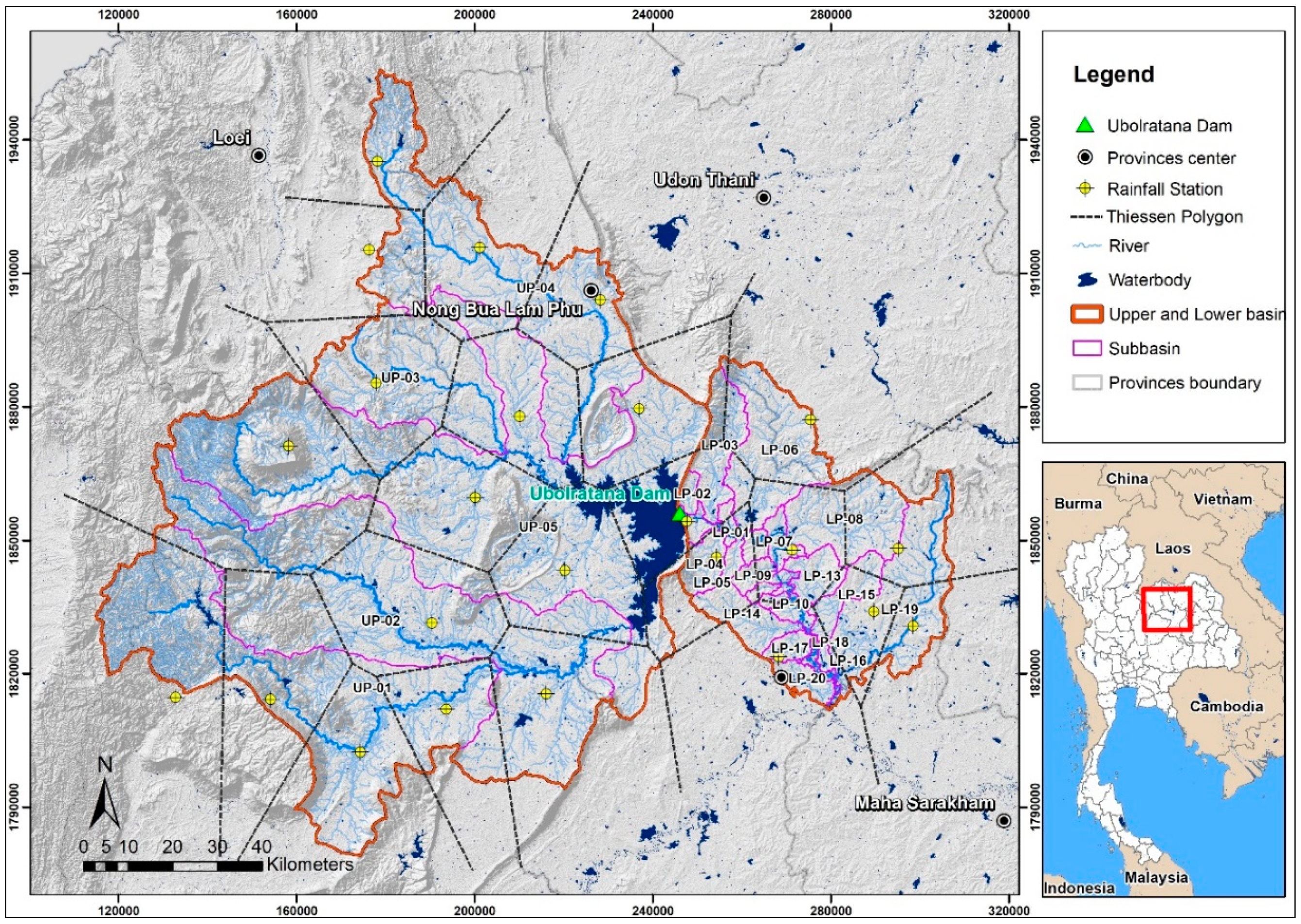
The study focused on the lower Nam Phong River Basin, which is located in the Northeastern region of Thailand, with a total area of approximately 2386 km², whereas the topography is undulating, varying in elevation from 139 m to 623 m above mean sea level (m+MSL) (note: since the Huai Sai Bat River is a main tributary of the Nam Phong River, the Huai Sai Bat sub-basin is then considered and included in this study, resulting in a larger study area of approximately 3127 km²). The Nam Phong River is considered to be the main river in the Nam Phong River Basin with a length of about 136 km that extends from the Ubol Ratana Dam (receiving the water from Lam Phaniang, Nam Phuai, Upper Lam Nam Phong, Lam Nam Choen, and Nam Phrom sub-basins with the storage capacity of 2431 million m³ (MCM)) at the upstream end to the Chi River at the downstream end (Figure 1). The climate in the river basin is typically dominated by monsoon winds, i.e., the Northeast monsoon brings cool and dry weather during November to February. A dry season prevails from March to May. After this, the wet season is characterized by the Southwest monsoon that lasts from June to October. The average annual temperature is 26.8 °C, ranging from about 16.7 °C in December to about 36.4 °C in April. The average relative humidity, for the year as a whole, is about 71.1%, in which the month with the highest relative humidity is September (82.5%) and the lowest is March (60%). The mean annual rainfall is approximately 1237.6 mm/year, whilst the month with most rainfall is September (224.9 mm) and the least is in January (2.1 mm) [18]. The mean annual discharge is about 1594.9 MCM/year with a minimum discharge of 34.5 MCM/year (in February) and a maximum discharge of 366.0 MCM/year (in October) [19].

2.2. Data Collection

The data collected for this study consists of 2 parts, which are 1) hydro-meteorological data, and 2) physical data of the river basin. Regarding the hydro-meteorological data, long-term daily datasets were collected from 24 rainfall stations of the Thai Meteorological Department (during 2000–2017), the E.22B gauging station (situated at Ban Tha Mao, Nam Phong District, Khon Kaen Province) of the Royal Irrigation Department (during 2005–2017), and the Ubol Ratana reservoir inflow hydrograph of the Electricity Generating Authority of Thailand (during 2005–2017) (see Figure 1 for locations of gauging stations). The physical river basin data such as the Digital Elevation Model (DEM, 5 m × 5 m grid spacing with vertical accuracies of 2 m for slope less than 35% and 4 m for slope greater than 35% [20]), land use, and soils were obtained from the Land Development Department (LDD). Other than that, the 2009 bathymetric surveys of 113 river cross sections at almost every 1 km along a 136 km reach of the Nam Phong River was also retrieved from the Research Center for Environmental and Hazardous Substance Management, Khon Kaen University.

2.3. GCMs, RCP Climate Scenarios, and Bias Correction

2.3.1. Representative Concentration Pathways (RCPs) Scenarios with Global Climate Models (GCMs) for South Asia (CORDEX-SA)

The analysis of future rainfall changes was used for the analysis of future streamflow calculated by the Hydrologic Engineering Center’s Hydrologic Modeling System (HEC-HMS) model. In this study, three sets of simulations were driven by the following three GCMs viz., CNRM-CM5, IPSL-CM5A-MR, and MPI-ESM-LR, for the future climate projections (see

Table 1. The description of the Global Climate Models (GCMs) downscaled by RCA4 CORDEX.

No	Driving GCM				RCM
	Name	Resolution (km)	Scenarios	Institute, Country	Name	Resolution (km)	Scenarios	Institute, Country
1	CNRM-CM5	155 × 155	RCP 4.5	CNRM-ERFACS, France	RCA4	50 × 50	RCP 4.5	SMHI, Sweden
			RCP 8.5				RCP 8.5
2	IPSL-CM5A-MR	275 × 275	RCP 4.5	IPSL, France	RCA4	50 × 50	RCP 4.5	SMHI, Sweden
			RCP 8.5				RCP 8.5
3	MPI-ESM-LR	210 × 210	RCP 4.5	MPI-M, Germany	RCA4	50 × 50	RCP 4.5	SMHI, Sweden
			RCP 8.5				RCP 8.5

for more details). Based on the model performance of historical runs, the downscaled future climate data was derived from the Regional Climate Model (RCM) with 50 km grid spacing under the influence of Representative Concentration Pathways (RCPs) 4.5 and 8.5 emission scenarios, from the Coordinated Regional Climate Downscaling Experiment over the South Asia Domain (CORDEX-SA) (note: RCP 4.5 represents a stable scenario where the radiative force will reach up to 4.5 W/m² by 2100) [21,22,23,24]. RCP 8.5 represents a relatively extreme scenario where greenhouse gas (GHG) will continuously increase throughout 2100, at which time radiative force will reach 8.5 W/m² [25,26].

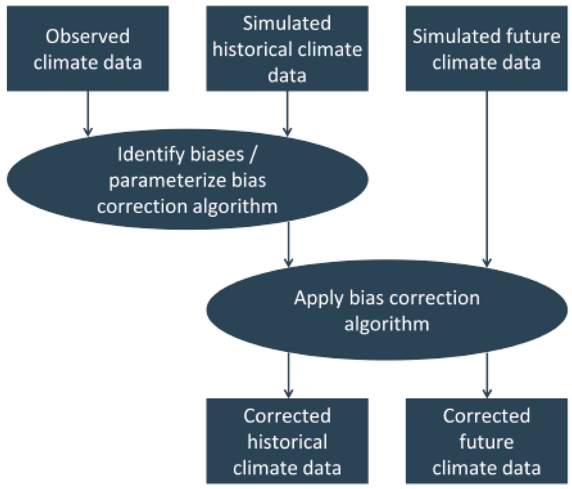
2.3.2. Bias Correction

The RCMs seem to be able to provide a higher spatial resolution and more reliable results on a regional scale in comparison to General Circulation Models (GCMs), as they can produce more spatially and physically coherent outputs with observations [27,28,29]. Nevertheless, the original RCM outputs still contain considerable bias due to the forcing of GCMs, or from systematic model errors, in which such biases could be amplified during climate change impact studies [30,31]. Therefore, the bias correction of RCM simulated data is of great importance and is a prerequisite step for data correction prior to climate change effect analysis. As such, the bias correction by the Linear Scaling method included in the tailor-made tool dubbed the “Climate Model data for hydrologic modeling (CMhyd)” was used for bias-correcting climate variables obtained from RCMs [32]. The RCMs simulated historical rainfall during the period of 1989–2005, which was calibrated with the historical observed rainfall during the same period, and projected rainfall for the period 2020–2039 under two RCPs (RCP 4.5 and RCP 8.5) (see Figure 2 for detailed bias correction procedure).

2.4. Analysis of Future Land Use Change

The analysis of future streamflow is based on the simulation results performed by HEC-HMS model, in which a parameter related to future land use would also need to be imported into the model for representing future runoff generation processes. In this study, the Land Change Modeler (LCM) tool, which is the extension of TerrSet software developed by Clark Lab [33], was used to analyze the spatial pattern of changes in predicting the Land Use and Land Cover (LULC) and validating the predicted LULC outputs [34]. A combination of Multi-Layer Perceptron (MLP) and Markov chain analysis was applied to model the transition and projection of historical (2010), present (2015), and future (2039) land use maps. The MLP, which is a feed-forward artificial neural network that generates a set of outputs from a set of inputs with separate training and recall phases [35], was trained to model land use transitions through creating transition maps. The transition potential maps created using MLP are based on a set of explanatory variables called drivers, i.e., agricultural areas, distance to urban areas, rivers, roads, as well as altitude, slope, and aspect of land. The land use modeling requires the integration of both changes in environmental and socio-economic drivers, however, the incorporation of the socio-economic factor is restricted by the lack of spatial data and the difficulties in integration with other environmental data [36]. The Markov chain method was also applied with sufficient accuracy to process the transition maps for the prediction process [37], based on the past trends of the land use changes from the period 2010 to 2015.

2.5. Hydrological Modeling

The estimation of streamflow in the Nam Phong River Basin was carried out using HEC-HMS model, which is designed for rainfall-runoff processes based on the relationships among runoff, evapotranspiration, infiltration, excess rainfall transformation, baseflow, and open channel routing of both gauged and ungauged river basins. In principle, the HEC-HMS program is a modeling system, which relies on dividing the hydrologic cycle into separate pieces, constructing watershed boundaries, and representing each water cycle component by a separate mathematical model. As a result, each mathematical model becomes suitable for different environments and conditions [38].

The HEC-HMS simulation results is stored in the HEC-DSS (Hydrologic Engineering Center’s Data Storage System), which can be used in conjunction with other HEC software, like Hydrologic Engineering Center’s River Analysis System (HEC-RAS), for water availability, urban drainage, flow forecasting, future urbanization impact, reservoir spillway design, flood damage reduction, floodplain regulation, and systems operation. More details on the process of HEC-HMS model construction are presented as follows.

2.5.1. Watershed Delineation

As a prerequisite to the HEC-HMS model set-up, the watershed was delineated and divided into several sub-basins using Arc Hydro Tools in ArcGIS 10.3 software, based on the 30-m Digital Elevation Model (DEM) and stream network. In consequence, the entire study area was then divided into 25 sub-basins consisting of 5 sub-basins for the upper Nam Phong River Basin (covering the areas upstream of the Ubol Ratana reservoir) and 20 sub-basins for the Lower Nam Phong River Basins (covering the areas downstream of the Ubol Ratana reservoir) (see more details in Figure 3).

2.5.2. HEC-HMS Hydrologic Elements

The HEC-HMS hydrologic elements, such as sub-basin, reach, junction, reservoir, diversion, source, and sink, are thoroughly connected in the river network, where their connectivity is considered to represent the runoff processes and their effects on the drainage system [38]. In this study, the Nam Phong model set-up contains only 5 of the abovementioned elements, accounting for in total 93 hydrologic elements. In detail, there are 25 sub-basin elements connected with 45 reaches and 22 junctions. In addition, five reservoir elements were also assigned to model the detention and attenuation of hydrographs caused by Ubol Ratana, Kaeng Sua Ten, Huai Siew, and Nong Loeng Yai Reservoirs, including Nong Wai Operation and Maintenance Project (Nong Wai Weir). A diversion element was also added to model the diverted flow from Nong Wai Weir to the left and right main irrigation canals.

2.5.3. Importing HEC-HMS Input Parameters

To estimate the water balance components, the following computation models were applied to the sub-basins and reaches in which their detailed descriptions can be described below.

• Runoff-volume models are used to compute the runoff volume of sub-basins by subtracting the rainfall by losses through interception, surface storage, infiltration, evaporation, and transpiration. In this study, the “Initial and constant rate model” was selected and used as sub-basin loss method for sub-basins within the Nam Phong River Basin.
• Direct-runoff models are used to convert excess rainfall into direct runoff at the outlets of each sub-basin. The “Snyder unit hydrograph model”, which is a synthetic unit hydrograph method developed to compute the peak flow as a unit of rainfall, was used in this study (note: a unit hydrograph represents the runoff distribution over time for one unit of rainfall excess over the entire watershed for a specified duration).
• Baseflow models are proposed to simulate the slow subsurface water drainage from the system into the channels, in which the “Exponential recession model” was chosen for this study.
• Routing models are employed to simulate one-dimensional open channel flow for determining the flow hydrograph at the downstream point of the sub-basin in relation to its upstream reach, and functions of sub-basin characteristics, such as slope and length of channel, channel roughness, channel shape, downstream control, and initial flow condition [39]. In this study, the “Muskingum model” was selected.

2.5.4. Importing Rainfall Data

The daily rainfall time-series during the period 2000–2017, collected from 24 selected weather stations of the Thai Meteorological Department (TMD) located within and surrounding the Nam Phong River Basin, was used in this study (see Figure 3 for rainfall station locations). Before importing rainfall data into the HEC-HMS model, the adjustment of point rainfall to areal rainfall distribution was made using the Thiessen Polygon Method, which is a standard method for computing mean areal rainfall for the topographical and meteorological homogeneous areas (see Equation (1) for formula used).

$$\overline{\mathrm{P}}=\frac{1}{\mathrm{A}}{\displaystyle \sum _{\mathrm{i}=1}^{\mathrm{n}}{\mathrm{P}}_{\mathrm{i}}{\mathrm{A}}_{\mathrm{i}}}$$

(1)

where

$\overline{\mathrm{P}}$—the mean areal rainfall

${\mathrm{P}}_{\mathrm{i}}$—rainfall observed at the i^th station inside or outside the Nam Phong River Basin

${\mathrm{A}}_{\mathrm{i}}$—in-region portion of the area of the polygon surrounding the i^th station (area of each polygon)

$\mathrm{A}$—the total area of the Nam Phong River Basin

$\mathrm{n}$—the number of areas

2.6. Frequency Analysis

Frequency analysis was used to estimate the time interval between similar size/intensity of events or the so-called return period of specific events. The frequently used probability function, i.e., Gumbel distribution, was used to estimate the probable (maximum daily and annual) rainfall in the Nam Phong River Basin for different return periods. The time horizon of 38 years was divided into periods of different lengths, i.e., the years 2000–2017 (baseline) and 2020–2039 (future). The RCM projected maximum daily rainfall for the period 2020–2039 was estimated for given return periods, i.e., 25-, 50-, and 100-year periods, based on a frequency–factor formulation of the Gumbel distribution (see Section 2.3.2 for details).

2.7. Hydraulic Modeling

The HEC-RAS hydraulic model, developed by the Hydrologic Engineering Center (HEC) of the U.S. Army Corps of Engineers, was used for flow and flood analysis under different discharge conditions in the river system of the Nam Phong River Basin, since the HEC-RAS set-up is capable of performing 1D steady state water surface profile calculations, as well as unsteady 1D and 2D flow simulations [40]. The water surface profiles are calculated from the previous cross section to the next one by solving the energy equation (Equation (2)) with an iterative procedure: the so-called standard step method [41] (note: the details of terms presented in Equation (2) can be seen in [38]). Furthermore, when carrying out the unsteady flow simulation, the HEC-RAS applies the continuity and momentum equations for determining the stage and flow at all locations in the model (see [38] for more details).

$${\mathrm{Z}}_2{+\mathrm{Y}}_2+\frac{{\mathrm{a}}_2{\mathrm{V}}_2^2}{2\mathrm{g}}={\mathrm{Z}}_1{+\mathrm{Y}}_1+\frac{{\mathrm{a}}_1{\mathrm{V}}_1^2}{2\mathrm{g}}+{\mathrm{h}}_{\mathrm{e}}$$

(2)

where

Z₁, Z₂—elevation of the main channel inverts

Y₁, Y₂—water depth at cross sections

V₁, V₂—average velocities

a₁, a₂—Saint Venant coefficients describing the variability of velocity profile in the particular cross section

g—gravitational acceleration

h_e—energy head loss

2.7.1. Schematic of the River System

To connect the river system, the schematic of the river system was firstly built using the geometric data editor available in HEC-RAS. Thereafter, the river system parts such as rivers, junctions, and additional hydraulic structures located along the rivers, can be properly depicted. All the values of the cross section, i.e., station, elevation, left and right overbanks, reach length, Manning’s roughness coefficients, left bank, right bank, and energy loss coefficients (friction, expansion, and contraction losses), must be entered, as the cross section describes the terrain profile of the river where the flooding on left/right banks can be clearly indicated.

2.7.2. Boundary Condition

Boundary conditions are required to establish the starting water surface for HEC-RAS to begin its calculations. The up- and downstream boundary conditions were entered for each reach, whereas the internal boundary conditions were defined for connections to junctions. The flow from each sub-basin determined by HEC-HMS hydrological model, together with the released flow from Ubol Ratana Dam stored in HEC Data Storage System (DSS), were imported into the HEC-RAS model through the unsteady flow data editor option. The diverted flow to irrigation canal system, which was assigned negative values, was also modelled to evaluate canal hydraulics for both steady and unsteady flow conditions. Regarding the downstream boundary condition, the type of boundary condition called “Normal Depth”, which is based on the assumption that the river flows under normal flow (uniform flow) conditions at the downstream boundary of the HEC-RAS set-up model, was selected. In detail, the normal depth or the stage for each computed flow was calculated based on Manning’s equation, by using the slope of the channel bottom, 0.00011 m/m.

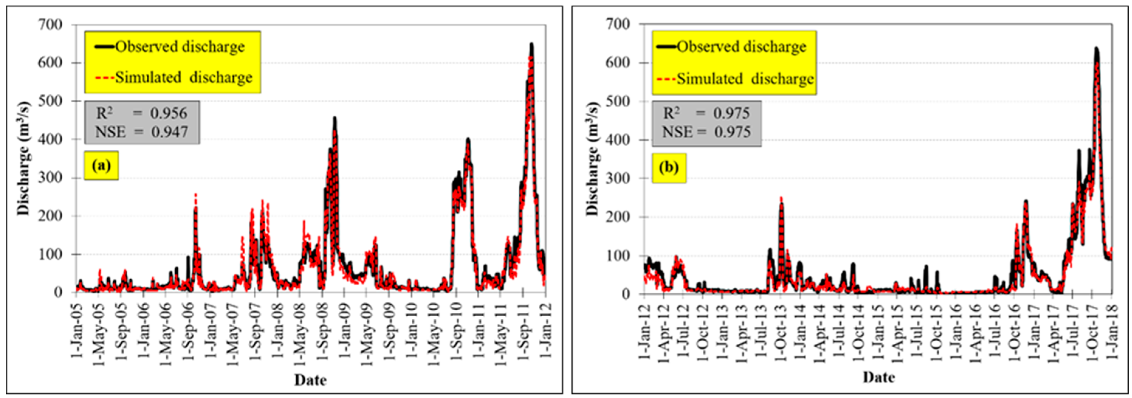
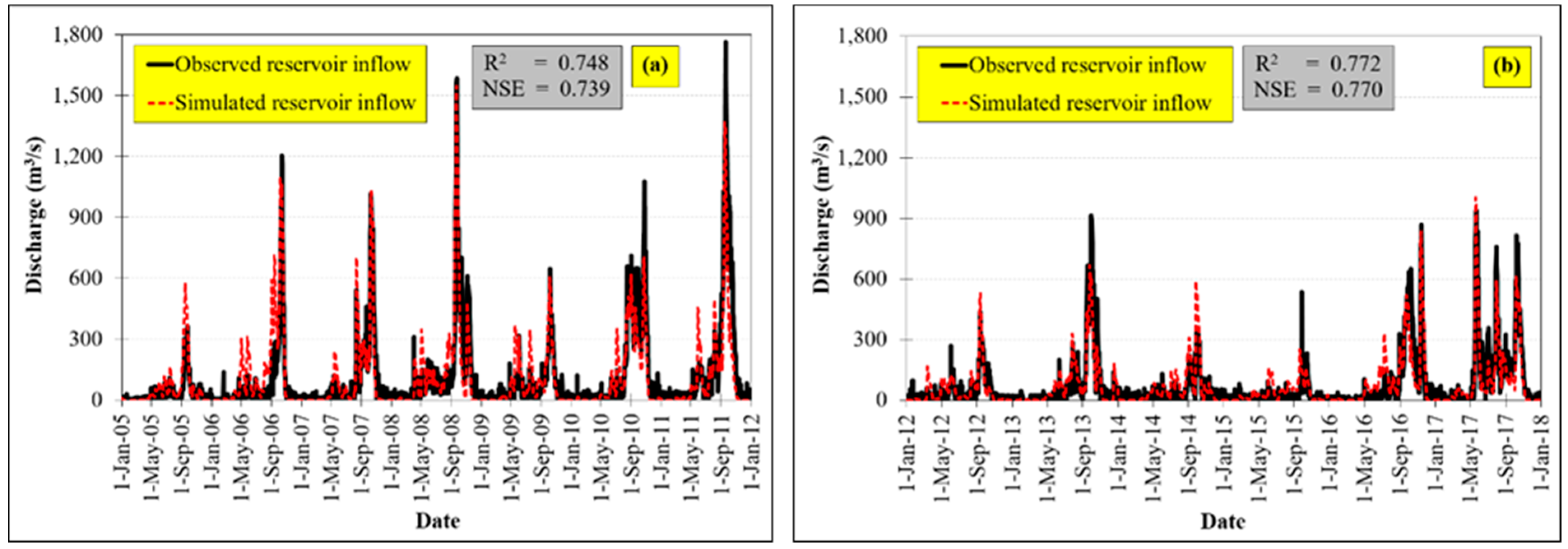
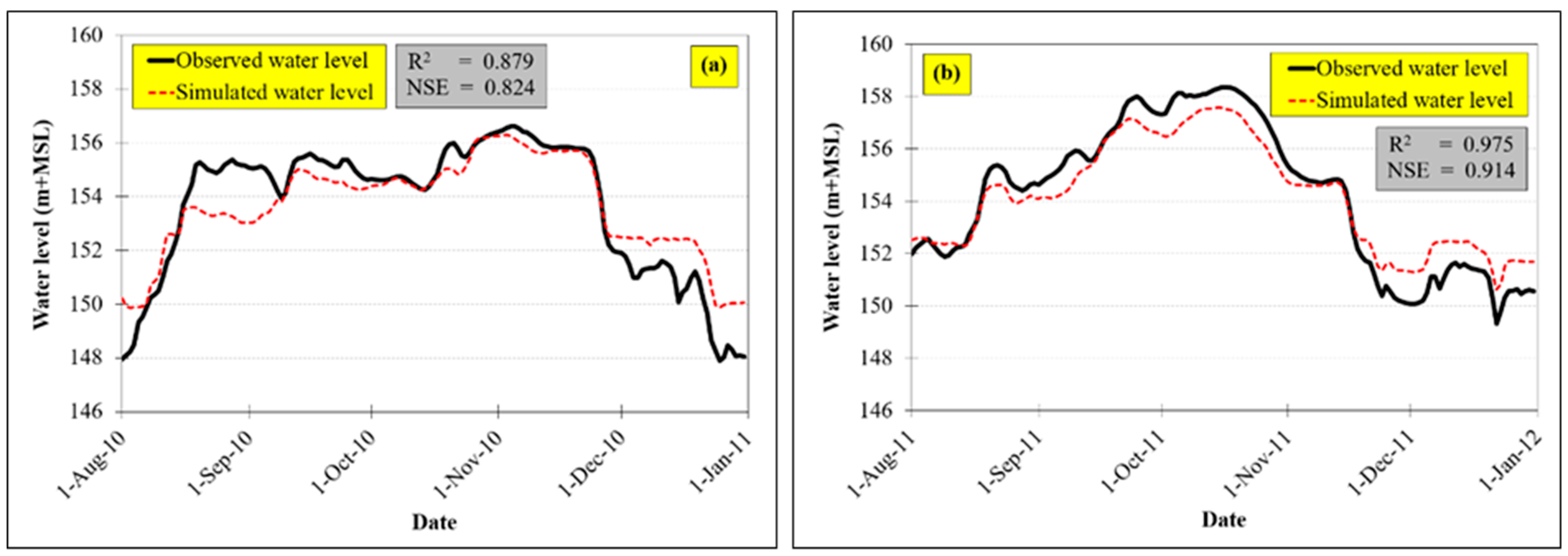
2.8. Model Calibration and Validation

The fundamental operation, the model calibration, was undertaken by adjusting/tuning identified sensitive parameters used in the HEC-HMS model at gauging station E.22B (discharge) and inflow to Ubol Ratana reservoir at a daily time-step during the period 2005 to 2011, and the 1D HEC-RAS model for daily water level at gauging station E.22B at a time-step during the flood period (August to December 2010) until the model simulation results closely match the observed values. In addition, the model evaluation procedure was also conducted through model validation process in order to prove that both set-up models are accurately capable of representing physical processes and providing predictive capabilities under different—though similar—conditions, based on a set of calibrated parameters and another set of hydrological data. For validation, the simulated outputs calculated by both models were also compared with the observed data at E.22B, i.e., daily discharge during the years 2012 to 2017 was used to validate the HEC-HMS, and daily water levels during the severe flood period (August to December 2011). The Coefficient of Determination (R²) and Nash–Sutcliffe Efficiency (NSE) [42], which are reliable criteria, were used to assess the goodness of both model performances during calibration and validation periods (see Equations (3) and (4) for the detailed formulas).

$${\mathrm{R}}^2={\left[\frac{{\displaystyle \sum _{\mathrm{i}=1}^{\mathrm{n}}\left({\mathrm{O}}_{\mathrm{i}}-{\mathrm{O}}_{\mathrm{avg}}\right)\left({\mathrm{P}}_{\mathrm{i}}-{\mathrm{P}}_{\mathrm{avg}}\right)}}{\left(\sqrt{{\displaystyle \sum _{\mathrm{i}=1}^{\mathrm{n}}{\left({\mathrm{O}}_{\mathrm{i}}-{\mathrm{O}}_{\mathrm{avg}}\right)}^2}}\right)\left(\sqrt{{\displaystyle \sum _{\mathrm{i}=1}^{\mathrm{n}}{\left({\mathrm{P}}_{\mathrm{i}}-{\mathrm{P}}_{\mathrm{avg}}\right)}^2}}\right)}\right]}^2$$

(3)

$$\mathrm{NSE}=1-\frac{{\displaystyle \sum _{\mathrm{i}=1}^{\mathrm{n}}{\left({\mathrm{O}}_{\mathrm{i}}-{\mathrm{P}}_{\mathrm{i}}\right)}^2}}{{\displaystyle \sum _{\mathrm{i}=1}^{\mathrm{n}}{\left({\mathrm{O}}_{\mathrm{i}}-{\mathrm{O}}_{\mathrm{avg}}\right)}^2}}$$

(4)

where

O_i—observed value at time-step i

O_avg—average observed value of the simulation period

P_i—simulated value at time-step i

P_avg—average simulated value of the simulation period

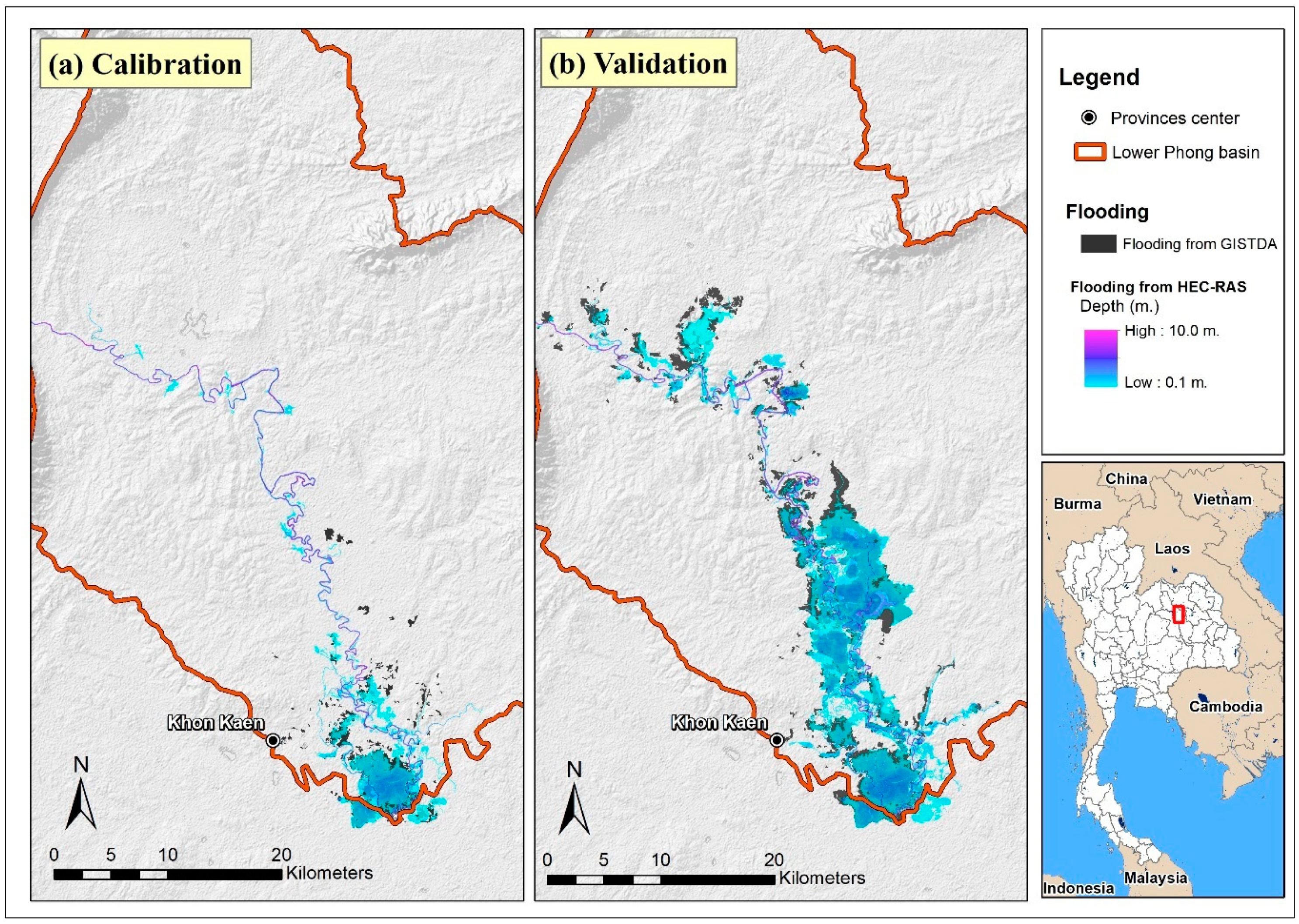
To precisely verify the results simulated by the 2D HEC-RAS model, the goodness of fit between the generated flood map from the HEC-RAS and the flood map extracted from the satellite images from Geo-Informatics and Space Technology Development Agency (Public Organization—GISTDA) was considered and assessed by the measure of Relative Error (RE) (Equation (5)), which is a measure that describes the percentage-difference between observed and simulated values over a specified time period and is useful in diagnostics of over-prediction or under-prediction (smaller values are the indication of better model performance). The F-statistics (F) (Equation (6)), which are the ratios of the area of the overlapping portion of the two flood extents to the area of both flood extents projected on the map, were also used to denote the overall goodness of fit of the HEC-RAS model simulations (a high F-statistic indicates very good model performance).

$$\mathrm{RE}=\frac{\left|{\mathrm{A}}_{\mathrm{o}}-{\mathrm{A}}_{\mathrm{p}}\right|}{{\mathrm{A}}_{\mathrm{o}}}$$

(5)

$$\mathrm{F}=\left(\frac{{\mathrm{A}}_{\mathrm{op}}}{{\mathrm{A}}_{\mathrm{o}}+{\mathrm{A}}_{\mathrm{p}}-{\mathrm{A}}_{\mathrm{op}}}\right)\times 100$$

(6)

where

${\mathrm{A}}_{\mathrm{o}}$—the inundation area extracted from satellite images

${\mathrm{A}}_{\mathrm{p}}$—the HEC-RAS generated flood inundation area

${\mathrm{A}}_{\mathrm{o}\mathrm{p}}$—the intersection of ${\mathrm{A}}_{\mathrm{o}}$ and ${\mathrm{A}}_{\mathrm{p}}$

2.9. Assessment of Flood Impacts and Damage

The amount of damage resulting from floods relies on flood characteristics, i.e., depth and duration. In this study, the flood damage assessment was performed based on direct damage estimation, which occurs as a consequence of the physical contact of floodwater with lives, properties, and any other objects. The damage functions derived by [43] (Equations (7) and (8)) were used for direct damage determination, in which four major types of land use were included in the calculation, i.e., residential, commercial, industrial, and agricultural. The list of coefficients for each land use type used in Equation (7) can be presented in

Table 2. Estimated flood damage coefficients for each different land use type [43].

No	Type	a0	a1	a2
1	Residential	−300.00	45.40	33.80
2	Commercial	−2.15	88.10	0.00
3	Industrial	−1740.00	522.00	181.00
4	Agriculture	−1050.00	553.00	0.00

.

$$\mathrm{DPE}={\mathrm{a}}_0+{\mathrm{a}}_1\mathrm{H}+{\mathrm{a}}_2\mathrm{L}$$

(7)

where

DPE—direct flood damage per land use type (Thai Baht)

H—maximum flood depth (cm)

L—flood duration (day)

a₀, a₁, a₂—flood damage coefficients (see Table 2)

The direct flood damage per land use type calculated by Equation (7) was then used to determine the direct flood damage for all land use types in Thai Baht by Equation (8).

$$\mathrm{DAM}={\displaystyle \sum }_{\mathrm{i}=1}^{\mathrm{n}}{\displaystyle \sum }_{\mathrm{j}=1}^4\frac{\mathrm{DPE}\left(\mathrm{j},\hspace{0.17em}\mathrm{H},\hspace{0.17em}\mathrm{L}\right)}{\mathrm{APE}\left(\mathrm{j}\right)}\cdot \mathrm{PC}\left(\mathrm{i}\hspace{0.17em},\hspace{0.17em}\mathrm{j}\right)\cdot \mathrm{AREA}\left(\mathrm{i}\right)$$

(8)

where

DAM—direct flood damage (Thai Baht)

DPE (j, H, L)—direct flood damage per land use type j at H, L (Thai Baht /land use type)

APE (j)—average area per land use type j per unit (m²) (see

Table 3. The average area per land use type per unit [44].

No	Type	Unit	Area Per Unit (m2)
1	Residential	Household	1000
2	Commercial	Shop	250
3	Industrial	Factory	4000
4	Agriculture	Farm	42,000

Note: The average household area per household (for residential area), average commercial area per shop (for commercial area), average industrial area per factory (for industrial area), and average agricultural area per farm (for agricultural area), were adjusted from the study of [45] in order to represent the actual land use situation of the lower Nam Phong River Basin.

)

PC (i, j)—percentage of land use type j in cell i (-)

AREA (i)—area of cell i (m²)

i—number of cell (-)

j—land use type 1, 2, 3, 4 (residential, commercial, industrial, agricultural) (-)

H—maximum flood depth (m)

L—flood duration (day)

It can be seen that the direct flood damage to infrastructure was excluded from the direct flood damage calculation. Therefore, as suggested by [46], the flood damage to infrastructure can be estimated at as high as 65% of the total direct flood damage, which enables the so-called “Total Direct Flood Damage (TDM)” to be calculated in Thai Baht (Equation (9)).

$$\mathrm{T}\mathrm{D}\mathrm{M}=\mathrm{D}\mathrm{A}\mathrm{M}+\left(0.65\cdot \mathrm{D}\mathrm{A}\mathrm{M}\right)$$

(9)

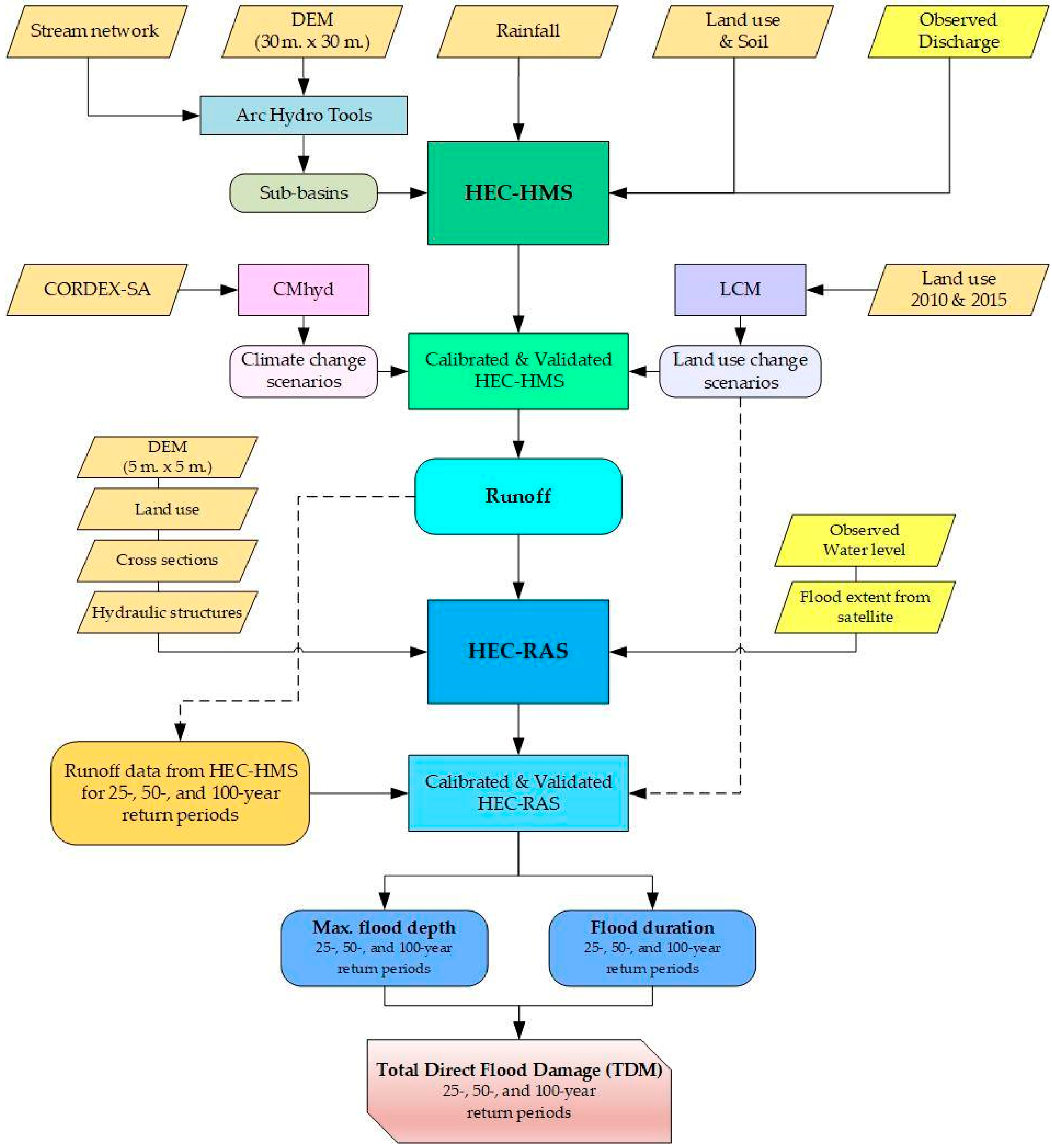
To achieve a better understanding from the above-detailed processes, the summarized key steps involved in the estimation of total direct flood damage of different return periods in the lower Nam Phong River Basin for land use and climate change scenarios are presented in Figure 4.

3. Results and Discussion

3.1. Analysis of Future Land Use Change

3.1.1. Identifying Trends of Land Use Changes

Two sets of land use data (2010 and 2015), which were classified into eleven land use categories, were used to identify trends of land use changes in the lower Nam Phong River Basin. Referring to

Table 4. Details of land use changes (km²) in the lower Nam Phong River Basin during the period of 2010 and 2015.

No	Land Use	Year 2010	Year 2015	Change
		Area (km2)	Area (km2)	km2	%
1	Aquaculture land	9.59	13.12	3.53	36.8
2	Field crop	3300.80	3582.42	281.62	8.5
3	Forest land	4621.29	4505.61	−115.68	−2.5
4	Horticulture	6.32	13.80	7.48	118.4
5	Miscellaneous land	633.19	557.42	−75.77	−12.0
6	Orchard	161.11	102.18	−58.93	−36.6
7	Paddy field	4351.11	4045.56	−305.55	−7.0
8	Pasture and farm house	22.68	19.74	−2.94	−13.0
9	Perennial crop	615.33	827.59	212.26	34.5
10	Urban and built-up land	705.99	757.36	51.37	7.3
11	Water body	611.12	613.73	2.61	0.4
Total		15,038.53	15,038.53

, it was found that the paddy field was decreased most significantly by 305.55 km², followed by the forested area, decreasing by 115.68 km², and miscellaneous land, decreasing by 75.77 km². The field (cash) crops, i.e., sugarcane and cassava, tended to be increased most markedly, by 281.62 km², and perennial crops (especially rubber trees) were the second largest increment by 212.26 km², and followed by the urban and built-up land with the increase about 51.37 km².

3.1.2. Projected Land Use Changes During the Period 2020–2039

Regarding the projected land use changes, the potential for land transitions was modeled using transition sub-models of LCM, which consist of a single land cover transition or a group of transitions with the same underlying driver variables [33]. In fact, the more transition sub-models used to generate suitable land use maps, the higher the simulation accuracy of the land use types of the lower Nam Phong River Basin, under the influence of the same driver variables. Therefore, in this study, seven transition sub-models including (1) field crop to urban and built-up land, (2) forest land to perennial crop, (3) forest land to urban and built-up land, (4) miscellaneous land to urban and built-up land, (5) paddy field to field crop, (6) paddy field to urban and built-up land, and (7) perennial crop to field crop, were considered for potential transition modeling. The changes in aquaculture land, horticulture, orchards, pastures and farmhouses, and water bodies were neglected for future projection of land use maps, because their transitions were found to be insignificant.

After the explorations of land use change trends, the possible future land use changes during the period 2020–2039 were investigated based on driver variables used for modeling the historical change process, i.e., agricultural areas, distance to urban areas, rivers, roads, as well as altitude, slope, and aspect of land. Upon the completion of the analysis conducted by LCM, in comparison to 2015 land use data, it was noticed that the projected paddy field in 2039 will be decreased significantly by 1278.40 km² (31.6%), whereas the forested area will also be decreased by 500.57 km² (11.1%). The field crop was found to be significantly increased by 1,803.32 km² (50.3%), whereas the next increment will be urban and built-up land for 268.86 km² (35.5%) (see

Table 5. The 2039 land use patterns in the lower Nam Phong River Basin compared to the 2015 land use data.

No	Land Use	Year 2015	Year 2039
		Area (km2)	Area (km2)	Change (km2)	Change (%)
1	Aquaculture land	13.12	13.12	0.00	0.0
2	Field crop	3582.42	5385.74	1803.32	50.3
3	Forest land	4505.61	4005.04	−500.57	−11.1
4	Horticulture	13.80	13.80	0.00	0.0
5	Miscellaneous land	557.42	525.48	−31.94	−5.7
6	Orchard	102.18	102.18	0.00	0.0
7	Paddy field	4045.56	2767.16	−1278.40	−31.6
8	Pasture and farmhouse	19.74	19.74	0.00	0.0
9	Perennial crop	827.59	566.32	−261.27	−31.6
10	Urban and built-up land	757.36	1026.22	268.86	35.5
11	Water body	613.73	613.73	0.00	0.0
Total		15,038.53	15,038.53

for more details). It can be observed that the development scenario changes in the future could either increase or decrease their land use changing rates, which are processed by the change analysis panel of LCM. As a result, based on the earlier land cover areas, the quantitative change of each land use type was determined by adding the gains and then subtracting the losses [47].

In this study, only four types of land use, i.e., residential, commercial, industrial, and agriculture, was used for flood impacts and damages assessment, as they are often at risk, with higher potential use, high possible damage costs, and high exposure to flooding. As such, the potential land use change analysis revealed that the agricultural land will have the largest decrease by 38.27 km² (1.7%), followed by the decrease of forested area by 49.76 km² (19.5%). The residential area was found to be increased by 95.62 km² (51.5%), whereas the industrial area was also found to be increased by 26.27 km² (245.1%) (see

Table 6. Trends in areas of the seven major land use categories in the lower Nam Phong River Basin between 2015 and 2039.

No	Land Use	Year 2015	Year 2039
		Area (km2)	Area (km2)	Change (km2)	Change (%)
1	Agricultural land	2253.40	2215.13	−38.27	−1.7
2	Commercial	47.81	54.17	6.36	13.3
3	Forest land	254.53	204.77	−49.76	−19.5
4	Industrial	10.72	36.99	26.27	245.1
5	Miscellaneous land	144.50	98.78	−45.72	−31.6
6	Residential	185.57	281.19	95.62	51.5
7	Water body	88.36	93.86	5.50	6.2
Total		2984.89	2984.89

for descriptions).

3.2. Analysis of Rainfall at Various Return Periods

In this study, the analysis of changes in rainfall was distinguished into the determination of daily maximum rainfall and annual rainfall at various return periods. The 18 years of data from historical simulation runs (2000–2017) were used as the baseline period, whereas the short-term future climate was represented by the 20-year period (2020–2039) from the scenario simulation runs. Three CMIP5 General Circulation Models, i.e., CNRM-CM5, IPSL-CM5A-MR, and MPI-ESM-LR, were downscaled, whereas the bias correction method, “linear scaling”, was used to adjust the climate models to better represent the observational data. Using the Gumbel distribution, the 25-, 50-, and 100-year return periods of daily maximum and annual rainfall were estimated for each of the CMIP5 GCMs and averaged over three GCMs under both RCP 4.5 and RCP 8.5 in the lower Nam Phong River Basin (see

Table 7. The 25-, 50-, and 100-year return periods of daily maximum rainfall (average from three CMIP5 GCMs) under RCP 4.5 and RCP 8.5 in the lower Nam Phong River Basin compared to baseline period (2000–2017).

Period	Scenario	Rainfall Peak (mm/day)
		25-yr	Relative Change (%)	50-yr	Relative Change (%)	100-yr	Relative Change (%)
2000–2017	Baseline	109.2		115.1		120.9
2020–2039	RCP 4.5	129.4	18.5	143.8	24.9	158.1	30.7
	RCP 8.5	119.2	9.1	130.7	13.5	142.1	17.5

and

Table 8. The 25-, 50-, and 100-year return periods of annual rainfall (average from three CMIP5 GCMs) under RCP 4.5 and RCP 8.5 in the lower Nam Phong River Basin compared to baseline period (2000–2017).

Period	Scenario	Annual Rainfall (mm/year)
		25-yr	Relative Change (%)	50-yr	Relative Change (%)	100-yr	Relative Change (%)
2000–2017	Baseline	1861.5		1994.6		2126.7
2020–2039	RCP 4.5	1783.4	−4.2	1911.3	−4.2	2038.4	−4.2
	RCP 8.5	1727.4	−7.2	1848.6	−7.3	1968.9	−7.4

).

3.3. Analysis of Runoff Simulated by HEC-HMS

3.3.1. Calibration and Validation of HEC-HMS

The HEC-HMS model calibration was carried out based on parameters identified during sensitivity analysis. The observed daily discharge time series at E.22B gauging station and the daily Ubol Ratana reservoir inflow was used for calibration, in which the dataset of 13 years was split into seven years (2005–2011) for calibration and six years (2012–2017) for validation. Regarding the evaluation criteria, the Coefficient of Determination (R²) and Nash–Sutcliffe Efficiency coefficient (NSE) were calculated and used to evaluate the HEC-HMS model performance, judging whether the model performance is satisfactory or unsatisfactory. For a daily time-step, the model is considered to be acceptable/satisfactory for the simulations of flow hydrograph for both gauged and ungauged river basins, when the values of R² and NSE are greater than 0.50 [48].

Based on the HEC-HMS calibrated parameters indicated in

Table 9. The summary of HEC-HMS calibrated parameters for the lower Nam Phong River Basin.

No	Method	Parameter	Calibrated Values
1	Simple Canopy	Initial Storage (%)	1.000
		Max Storage (mm)	100.000
		Crop Coefficient	1.000
2	Simple Surface	Initial Storage (%)	1.000
		Max Storage (mm)	50.000
3	Initial and constant rate	Initial Loss (mm)	3.660–11.220
		Constant Rate (mm/h)	0.240–0.892
		Impervious (%)	2.650–37.570
4	Snyder Unit hydrograph	Lag Time (h)	0.100–41.15
		Peaking Coefficient	0.100–0.300
5	Exponential recession	Recession Constant	5.000
		Ratio of Peak	5.000
6	Muskingum	Muskingum K (h)	0.020–4.550
		Muskingum X	0.250

, the model calibration and validation results showed a reasonable match between observed and simulated hydrographs (see Figure 5 and Figure 6). In detail, at the E.22B gauging station, the R² and NSE values were found to be 0.956 and 0.947, respectively, for calibration, whereas the R² and NSE values reached the same values of 0.975, for validation. By considering the daily Ubol Ratana reservoir inflow, the R² and NSE values were 0.748 and 0.739, respectively, for calibration, whereas the R² and NSE values were 0.772 and 0.770, respectively, for validation. The overall performance and capabilities of the HEC-HMS make it a superior model well-suited for assessing the impacts of future climate and land use change scenarios on streamflow in the lower Nam Phong River Basin.

3.3.2. Analysis of Baseline and Future Peak Discharges Under Different Return Periods

By importing the daily maximum rainfall and annual rainfall of each CMIP5 model indicated in Table 7 and Table 8, and the projected future land use into the HEC-HMS model, the hydrological simulations under different scenarios were conducted. At the outlet of the lower Nam Phong River Basin, the maximum daily outflow discharges for each of three CMIP5 GCMs and the average maximum daily outflow discharges for average three GCMs (CNRM-CM5, IPSL-CM5A-MR, and MPI-ESM-LR) under both RCP 4.5 and RCP 8.5 at different time periods (2000–2017 and 2020–2039), were then obtained as can be seen in

Table 10. The average maximum daily outflow discharges at the outlet of the lower Nam Phong River Basin for average three Coupled Model Intercomparison Project Phase 5 (CMIP5) GCMs under both Representative Concentration Pathway (RCP) 4.5 and RCP 8.5 at different time periods.

Period	Scenario	Average Maximum Daily Outflow Discharge (m3/s)
		25yr	Relative Change (%)	50yr	Relative Change (%)	100yr	Relative Change (%)
2000–2017	Baseline	1051.6	-	1169.0	-	1273.6	-
2020–2039	RCP4.5	909.6	−13.5%	1017.4	−13.0%	1112.3	−12.7%
2020–2039	RCP8.5	1162.7	10.6%	1299.5	11.2%	1436.5	12.8%

.

3.4. Analysis of Hydraulic Variables Simulated by HEC-RAS

3.4.1. Calibration of HEC-RAS

The calibration process was performed by using both recorded water level time series and historical flood extent. To enable a good match between observed and simulated water levels and delineated flood extents for given flow events, the key parameter to be adjusted during the calibration phase is the Manning’s roughness coefficient (Manning’s n) of the river channel and floodplain. The closeness of fit between the compared water levels was evaluated using two statistical indicators, i.e., the values of Coefficient of Determination (R²) and Nash–Sutcliffe Efficiency (NSE), which are used to evaluate the overall performance of the calibrated HEC-RAS model (note: the model is judged to be acceptable or satisfactory when the values of R² and NSE are greater than 0.50 [49]). More detailed calibration results are presented below.

The Calibration of Daily Water Level

The calibration was completed during the flood period (August to December 2010), by raising or lowering the Manning’s n values for both river channel and floodplain, until the best fit between observed and simulated water levels at the E.22B gauging station was achieved as revealed by the R² and NSE of 0.879 and 0.824, respectively. A reasonably good agreement among water levels can be seen in Figure 7a.

The Calibration of Delineated Flood Extents

The map of flood extent was delineated by the post-processing of simulated results of the HEC-RAS. The Manning’s n values were varied during this calibration process in order to match the simulated flood extents with satellite observed ones. Eventually, a comparison of simulated and observed maximum flood extents from GISTDA for the October 2010 flood event was created, as illustrated in Figure 8a.

The graphical method (visual observation) and values of statistical parameters, i.e., Relative Error (RE) and F-statistics (calculated by Equations (5) and (6)), were used as an indication of calibration acceptance. Notably, the simulated flood extent seems to be in good agreement with the observed one, as can be seen from a good match between the flood extent boundaries during the maximum flood condition (on 31 October 2010). Referring to Jung et al. (2014), the values of Relative Error (RE) of 0.05 (with a value closer to zero meaning that no overlapping portion for two flood inundations), and the F-statistic of 43.55% (with high F-statistics indicates the goodness of fit between two flood inundations), also confirm that the calibrated HEC-RAS model is useable for flood extent delineation.

3.4.2. Validation of HEC-RAS

To ensure the accuracy and robustness of HEC-RAS model, the validation was carried out by running the model with the calibrated n-values using different observed datasets than those used for calibration. The monitoring (observation) of the water level and the flood extent derived from satellite images by GISTDA were used as validation targets to demonstrate the suitability and effectiveness of the calibrated HEC-RAS model for flood hazard assessment in the lower Nam Phong River Basin. More details on validation results are summarized as follows.

The Validation of Daily Water Level

The validation was conducted with field water level measurements at the E.22B gauging station, in which the selected validation period was from 1 August to 31 December 2011. Referring to Figure 7b, the R² and NSE were reasonably determined to be 0.975 and 0.914, respectively (more than 0.50 as recommended by [49]), which corresponds to a perfect match of the modelled daily water level from the observed data.

The Validation of Delineated Flood Extents

Based on the calibrated Manning’s n values, the validation for the calibrated HEC-RAS model was performed for the 2011 flood period. The validation results were found to be satisfactory, as can be observed from the good match between observed flood inundation extent obtained from GISTDA and the flood extent map extracted from the HEC-RAS, with a low Relative Error (RE) of 0.10 and a high F-statistics of 47.89% (see Figure 8b).

According to the above-measured performance, it can be said that the calibrated HEC-RAS model can perfectly simulate the complicated hydraulic behavior of rivers and floodplains and provide satisfied/valid results.

3.5. Results of Flood Damage Assessment

Assessment of Flood Damage for Different Return Periods

The assessment of flood damage was based on the direct flood damage per land use type (DPE) as calculated by Equation (7). The map overlaying technique of raster data format (storing spatial information) in ArcGIS 10.3 software was applied for flood damage estimation of the lower Nam Phong River Basin. The new map themes were created with a geoprocessing tool called “Raster Calculator” function within the ArcGIS framework, which allows for complex mathematical calculations to be made on rasters. Initially, the 5 m × 5 m raster layers of maximum flood depth (H) and flood duration (L) obtained from the HEC-RAS, including land use for each scenario, were imported into ArcGIS. The raster calculator function was then employed to calculate the direct flood damage per land use type (DPE in Thai Baht) based on flood damage coefficients (a0, a1, and a2).

The direct flood damage in Thai Baht (DAM) was then calculated by multiplying the direct flood damage per land use type (DPE) with the area of cell (5 m × 5 m cell size) and the percentage of land use type in specified cell (equal to one as each raster cell contains only one land use type), and divided by the average area per land use type per unit area (APE) (See Equation (8)).

In addition, there is no doubt about the fact that flood damage to infrastructure is of vital importance, as it can cause both short and long-term impacts, i.e., disruptions to electricity and water supply, transportation, communication, education, and health facilities. Therefore, the direct flood damage to infrastructure must be included in the direct flood damage calculation, which is 65% of the total direct flood damage, and leading to the total direct flood damage (TDM) (see Equation (9)).

Table 11. Estimation of total direct flood damage in the lower Nam Phong River Basin at different return periods for both baseline and future climate scenarios.

Period	Scenario	Land Use Type	Total Direct Flood Damage (TDM)
			25yr		50yr		100yr
			(million US$)	(%)	(million US$)	(%)	(million US$)	(%)
2000–2017	Baseline		10.52	100.00	11.50	100.00	12.69	100.00
		Residential	0.72	6.80	0.79	6.85	0.85	6.73
		Commercial	0.41	3.86	0.44	3.85	0.46	3.63
		Industrial	0.27	2.53	0.28	2.43	0.28	2.24
		Agriculture	4.99	47.41	5.46	47.50	6.09	48.00
		Infrastructure	4.14	39.39	4.53	39.37	5.00	39.39
2020–2039	RCP 4.5		14.84	100.00	16.91	100.00	18.02	100.00
		Residential	3.51	23.65	3.93	23.22	4.19	23.24
		Commercial	0.55	3.72	0.71	4.19	0.76	4.20
		Industrial	0.44	2.94	0.52	3.05	0.54	2.99
		Agriculture	4.50	30.30	5.10	30.14	5.44	30.17
		Infrastructure	5.85	39.39	6.66	39.39	7.10	39.39
	RCP 8.5		16.24	100.00	17.40	100.00	18.67	100.00
		Residential	3.73	22.95	4.03	23.16	4.33	23.21
		Commercial	0.68	4.22	0.70	4.01	0.73	3.93
		Industrial	0.49	3.02	0.52	3.00	0.53	2.82
		Agriculture	4.94	30.41	5.30	30.44	5.72	30.64
		Infrastructure	6.40	39.41	6.85	39.39	7.35	39.39

Note: Exchange rate is as of August 6, 2019 (US$1 = 30.766 Baht).

shows the total direct flood damage of different return periods and time horizons in the lower Nam Phong River Basin for both the baseline and future climate scenarios.

It can be noted that in Table 11, the direct flood damages significantly increase with higher return periods for both the baseline and future conditions. Damages of 10.52, 11.50, and 12.69 million US$ are found for 25-, 50-, and 100-year return periods, respectively, under the baseline scenario. Regarding the future period, the damages are found to be 14.84, 16.91, and 18.02 million US$ for return periods of 25-, 50-, and 100-year, respectively, under the RCP 4.5 scenario, which is less than the damages under RCP 8.5, i.e., 16.24, 17.40, and 18.67 million US$, respectively. Other than that, when considering each type of land use, the agriculture is found to be the most devastated by floods during the baseline period by approximately 48% of the total direct flood damage, following by infrastructure (about 40%), residential area (almost 7%), and the rest. Under two emission scenarios (RCPs 4.5 and 8.5), the majority of direct flood damage is still found to be agricultural with somewhat of a decrease from the baseline by roughly 18%, due to the conversion from agricultural to residential (highest increase from the baseline by nearly 17%), commercial, and industrial development. The results can also be shown in the forms of the relationship among four different variables, i.e., 1) flood stage at E.22B gauging station, 2) maximum released flow from Ubol Ratana Dam, 3) probability or likelihood of flood occurrence (inverse of the return period), and 4) total direct flood damage. For ease of viewing, the relationship is presented by different time horizons and emission scenarios as can be seen in Figure 9. The logic of this figure moves counterclockwise starting from the upper right corner and ending in the lower right corner. Firstly, the northeast quadrant describes the probability or likelihood of flood occurrence equal to or greater than the maximum released flow from the Ubol Ratana Dam occurring within a given time period. Next, the relationship between flood stage at E.22B gauging station and maximum released flow from Ubol Ratana Dam is presented in the northwest quadrant, which describes how high the flood stage at E.22B gauging station might be for a given maximum released flow from the Ubol Ratana Dam. After this, the amount of flood damage that might occur in the lower Nam Phong River Basin, in relation to a certain flood stage at the E.22B gauging station is shown in the southwest quadrant. Eventually, the southeast quadrant relates the expected flood damage that might occur in the lower Nam Phong River Basin to the probability of flood occurrence.

4. Conclusions

In this study, the potential climate and land use change impacts on floods in the selected case study, the lower Nam Phong River Basin, was undertaken using HEC-HMS hydrological and HEC-RAS hydraulic models under different return periods and future emission scenarios. The future climate change was projected for the years 2020–2039 (early century) in comparison to the baseline period of 2000–2017, under a set of Representative Concentration Pathway (RCP) greenhouse gas scenarios (RCPs 4.5 and 8.5) from CMIP5 model simulations, i.e., CNRM-CM5, IPSL-CM5A-MR, and MPI-ESM-LR. The high resolution downscaled (50-km grid spacing) and bias corrected daily rainfall was then used as an input for the calibrated HEC-HMS model (periods of 2005–2011 and 2012–2017 for calibration and validation, respectively) to generate a future daily discharge time series, in which the flood inundation maps were obtained by the calibrated HEC-RAS model (wet periods of 2010 and 2011 for calibration and validation, respectively).

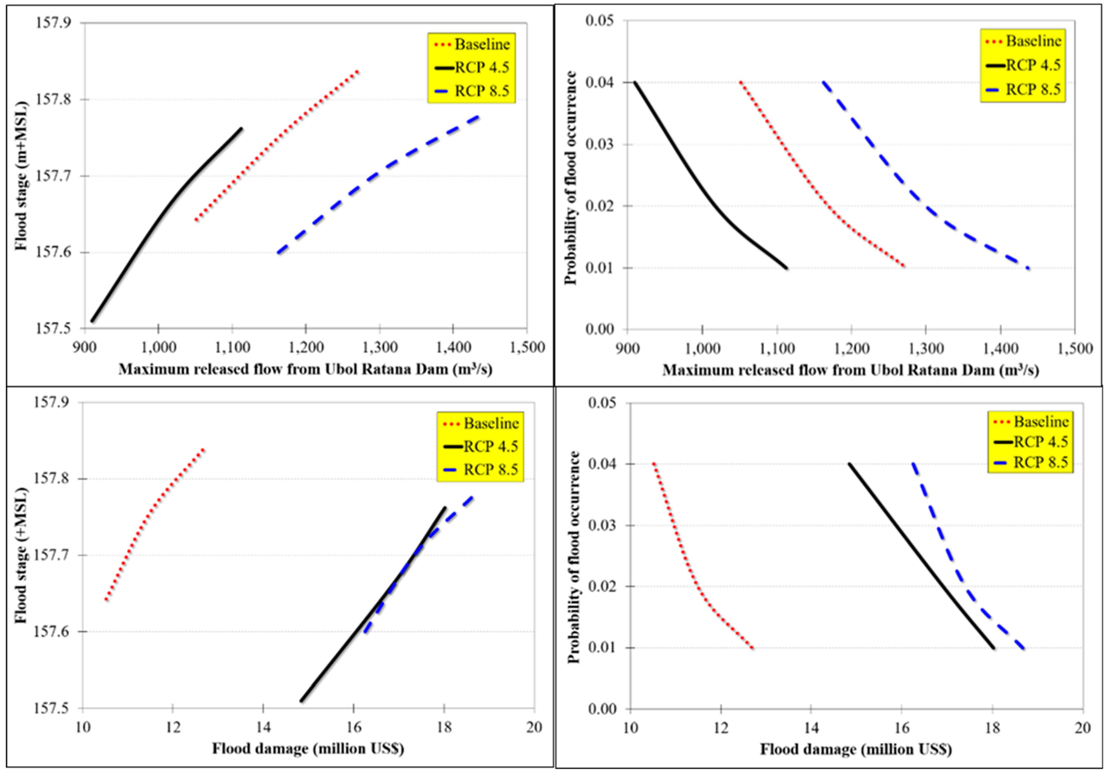
The simulation findings revealed that, during the period 2000–2017, the potential flooded area in the lower Nam Phong River Basin with 25-, 50-, and 100-year return periods are 140.95 km², 150.45 km², and 165.33 km², respectively, meanwhile the 2011 flood extent is about 128.08 km². In view of future scenarios, the extent of flood inundation under RCP 4.5 is smaller than the baseline case for 25-, 50-, and 100-year return periods by 4.97 km², 1.01 km², and 8.59 km², respectively, whereas the flood extent under RCP 8.5 is larger than the baseline condition for 25- and 50-year return periods by 5.30 km² and 3.86 km², respectively, and almost no difference is found for the 100-year return period. The severity of flood events is projected to be increased and is likely to be serious in the RCP 8.5 scenario rather than RCP 4.5 scenario. There is little difference, in fact, in flood extent between the baseline and future cases, nevertheless, it is obvious that the future flood duration tends to increase. The inundation extent with zero to two months of flood duration is likely to decrease, whereas the extent with four to six months of flood duration is expected to be increased, especially for high return periods.

By considering the maximum flood depth and flood duration into the calculation of total direct flood damage, the direct flood damage clearly increases, with higher return periods for both the baseline and future conditions. With respect to the baseline, the total direct damage is estimated at 10.52, 11.50, and 12.69 million US$ at the 25-, 50-, and 100-year return periods, respectively. In terms of future conditions, the total direct damage under RCP 4.5 is expected to be 14.84, 16.91, and 18.02 million US$ for the 25-, 50-, and 100-year return periods, respectively, whereas the total direct damage under RCP 8.5 is found to be higher by 1.40, 0.49, and 0.65 million US$, respectively. In addition, most of the total direct flood damage is in agriculture, followed by infrastructure and residential area, for both the baseline and future scenarios. However, the future agricultural damage is detected to be decreased from the baseline by approximately 18%, while the future damage for residential (expected to be increased from the baseline of up to 17%), commercial, and industrial areas tend to be increased from the baseline. Above all, it can be said that the future flood damage tends to increase because of changes in climate, together with the effect of increased exposure due to land use conversion.

Finally, the main findings from this study should prove very useful for defining and directing effective adaptation strategies to limit potential flood risks in the lower Nam Phong River Basin to a low level, both in probability and damage. The findings also could be used as a guideline for other areas throughout Thailand.

References

1. USAID (United States Agency for International Development). Southeast Asia Floods Fact Sheet #1. Available online: https://pdf.usaid.gov/pdf_docs/PA00J4C8.pdf (accessed on 3 February 2020).
2. Imudom, W.; Phongpiyaphaiboon, N.; Suvattanametakul, C.; Jitsutthiphakorn, U.; Vibulsrisajja, T. Thailand Floods 2011: Impact and Recovery from Business Survey; Bank of Thailand: Bangkok, Thailand, 2012. [Google Scholar]
3. Thai Meteorological Department. Annual Weather Summary of Thailand in 2011; Thai Meteorological Department: Bangkok, Thailand, 2012.
4. Gale, E.L.; Saunders, M.A. The 2011 Thailand Flood: Climate Causes and Return Periods. Weather 2013, 68, 233–237. [Google Scholar] [CrossRef] [Green Version]
5. Bunya, J.; Tang, C.S. Resilient Response and Recovery at Western Digital: After the Thai Flood. Available online: https://www.thecasecentre.org/educators/products/view?&id=114608 (accessed on 3 February 2020).
6. World Bank. Thai Flood 2011: Rapid Assessment for Resilient Recovery and Reconstruction Planning; The World Bank: Bangkok, Thailand, 2012; pp. 1–36. [Google Scholar]
7. Prasanchum, H.; Kangrang, A.; Hormwichian, R.; Compliew, S. Impact of Climate and Rapid Land Use Changes on Runoff Quantities in Lower-Lampao River Basin. Mahasarakham Int. J. Eng. Technol. 2016, 2, 1–5. [Google Scholar]
8. Chacuttrikul, P.; Kiguchi, M.; Oki, T. Impacts of Climate and Land Use Changes on River Discharge in a Small Watershed: A Case Study of the Lam Chi Subwatershed, Northeast Thailand. Hydrol. Res. Lett. 2018, 12, 7–13. [Google Scholar] [CrossRef]
9. Shrestha, S.; Lohpaisankrit, W. Flood Hazard Assessment under Climate Change Scenarios in the Yang River Basin, Thailand. Int. J. Sustain. Built Environ. 2017, 6, 285–298. [Google Scholar] [CrossRef] [Green Version]
10. Bai, Y.; Zhang, Z.; Zhao, W. Assessing the Impact of Climate Change on Flood Events using HEC-HMS and CMIP5. Water. Air. Soil Pollut. 2019, 230, 119. [Google Scholar] [CrossRef]
11. Azmat, M.; Qamar, M.U.; Huggel, C.; Hussain, E. Future Climate and Cryosphere Impacts on the Hydrology of a Scarcely Gauged Catchment on the Jhelum River Basin, Northern Pakistan. Sci. Total Environ. 2018, 639, 961–976. [Google Scholar] [CrossRef]
12. Kheereemangkla, Y.; Shrestha, R.P.; Shrestha, S.; Jourdain, D. Modeling Hydrologic Responses to Land Management Scenarios for the Chi River Sub-basin Part II, Northeast Thailand. Environ. Earth Sci. 2016, 75, 793. [Google Scholar] [CrossRef]
13. Pruethong, C.; Kuntiyawichai, K.; Sri-Amporn, W.; Jothityangkoon, C. Impacts of Land Use and Rainfall Frequency Changes on Peak Discharges and Inundation Areas in the Lower Nam Phong River Basin. Naresuan Univ. Eng. J. 2019, 14, 113–126. [Google Scholar]
14. Singkran, N.; Tosang, J.; Waijaroen, D.; Intharawichian, N.; Vannarart, O.; Anantawong, P.; Kunta, K.; Wisetsopa, P.; Tipvong, T.; Janjirawuttikul, N.; et al. Influences of Land Use and Climate Changes on Hydrologic System in the Northeastern River Basin of Thailand. J. Water Clim. Chang. 2015, 6, 325–340. [Google Scholar] [CrossRef]
15. Shrestha, S. Assessment of Water Availability under Climate Change Scenarios in Thailand. J. Earth Sci. Clim. Chang. 2014, 5, 1–8. [Google Scholar] [CrossRef]
16. Sukwimolseree, T.; Kosa, P. The Relationship between Land Use Change and Runoff. Int. J. Environ. Ecol. Eng. 2014, 8, 428–431. [Google Scholar]
17. Homdee, T.; Pongput, K.; Kanae, S. Impacts of Land Cover Changes on Hydrologic Responses: A Case Study of Chi River Basin, Thailand. J. Jpn. Soc. Civ. Eng. Ser. B1 Hydraul. Eng. 2011, 67, I_31–I_36. [Google Scholar] [CrossRef] [Green Version]
18. Secretariat Office of the Chi River Basin Committee. Management of the Chi River Basin; Water Resources Regional Office 4, Department of Water Resources, Ministry of Natural Resources and Environment: Khon Kaen, Thailand, 2012.
19. Kuntiyawichai, K.; Sri-Amporn, W.; Pruthong, C. Quantifying Consequences of Land Use and Rainfall Changes on Maximum Flood Peak in the Lower Nam Phong River Basin. Available online: https://www.scientific.net/AMR.931-932.791 (accessed on 3 February 2020).
20. Land Development Department. Products from MOAC’s Natural Resources and Properties Administration project. Available online: http://www.ldd.go.th/web_eng56/Main_project/Products%20%20from%20MOAC%E2%80%99s%20Natural%20resources.html (accessed on 14 March 2020).
21. Wise, M.; Calvin, K.; Thomson, A.; Clarke, L.; Bond-Lamberty, B.; Sands, R.; Smith, S.J.; Janetos, A.; Edmonds, J. Implications of Limiting CO2 Concentrations for Land Use and Energy. Science 2009, 324, 1183–1186. [Google Scholar] [CrossRef] [PubMed]
22. Clarke, L.; Edmonds, J.; Jacoby, H.; Pitcher, H.; Reilly, J.; Richels, R. Scenarios of Greenhouse Gas Emissions and Atmospheric Concentrations; U.S. Climate Change Science Program; Subcommittee on Global Change Research; Department of Energy, Office of Biological & Environmental Research: Washington, DC, USA, 2007; p. 164.
23. Smith, S.J.; Wigley, T.M. Multi-Gas Forcing Stabilization with the MiniCAM. Energy J. Spec. 2006. [Google Scholar] [CrossRef]
24. Guisan, A.; Thuiller, W. Predicting Species Distribution: Offering more than Simple Habitat Models. Ecol. Lett. 2005, 8, 993–1009. [Google Scholar] [CrossRef]
25. Meinshausen, M.; Smith, S.J.; Calvin, K.; Daniel, J.S.; Kainuma, M.L.T.; Lamarque, J.-F.; Matsumoto, K.; Montzka, S.A.; Raper, S.C.B.; Riahi, K.; et al. The RCP Greenhouse Gas Concentrations and their Extensions from 1765 to 2300. Clim. Chang. 2011, 109, 213. [Google Scholar] [CrossRef] [Green Version]
26. Riahi, K.; Grübler, A.; Nakicenovic, N. Scenarios of Long-term Socio-economic and Environmental Development under Climate Stabilization. Technol. Forecast. Soc. Chang. 2007, 74, 887–935. [Google Scholar] [CrossRef]
27. Buonomo, E.; Jones, R.; Huntingford, C.; Hannaford, J. On the Robustness of Changes in Extreme Precipitation over Europe from Two High Resolution Climate Change Simulations. Q. J. R. Meteorol. Soc. 2007, 133, 65–81. [Google Scholar] [CrossRef]
28. Chen, J.; Brissette, F.P.; Chaumont, D.; Braun, M. Performance and Uncertainty Evaluation of Empirical Downscaling Methods in Quantifying the Climate Change Impacts on Hydrology over Two North American River Basins. J. Hydrol. 2013, 479, 200–214. [Google Scholar] [CrossRef]
29. Turco, M.; Llasat, M.C.; Herrera, S.; Gutiérrez, J.M. Bias Correction and Downscaling of Future RCM Precipitation Projections using a MOS-Analog Technique. J. Geophys. Res. Atmos. 2017, 122, 2631–2648. [Google Scholar] [CrossRef] [Green Version]
30. Durman, C.F.; Gregory, J.M.; Hassell, D.C.; Jones, R.G.; Murphy, J.M. A Comparison of Extreme European Daily Precipitation Simulated by a Global and a Regional Climate Model for Present and Future Climates. Q. J. R. Meteorol. Soc. 2001, 127, 1005–1015. [Google Scholar] [CrossRef]
31. Herrera, S.; Fita, L.; Fernández, J.; Gutiérrez, J.M. Evaluation of the Mean and Extreme Precipitation Regimes from the ENSEMBLES Regional Climate Multimodel Simulations over Spain. J. Geophys. Res. Atmos. 2010, 115. [Google Scholar] [CrossRef] [Green Version]
32. Rathjens, H.; Bieger, K.; Srinivasan, R.; Chaubey, I.; Arnold, J.G. CMhyd User Manual: Documentation for Preparing Simulated Climate Change Data for Hydrologic Impact Studies. Available online: https://swat.tamu.edu/media/115265/bias_cor_man.pdf (accessed on 6 January 2020).
33. Eastman, J.R. Terrset Geospatial Monitoring and Modeling System; Clark Labs, Clark University: Worcester, MA, USA, 2016. [Google Scholar]
34. Gupta, R.; Sharma, L.K. Efficacy of Spatial Land Change Modeler as A Forecasting Indicator for Anthropogenic Change Dynamics over Five Decades: A Case Study of Shoolpaneshwar Wildlife Sanctuary, Gujarat, India. Ecol. Indicat. 2020, 112, 1–19. [Google Scholar] [CrossRef]
35. Wasserman, T.; Wasserman, L.D. Therapy and the Neural Network Model, Neural Network Model: Applications and Implications; Springer: Cham, Switzerland, 2019; p. 200. [Google Scholar]
36. Veldkamp, A.; Lambin, E.F. Predicting Land-use Change. Agric. Ecosyst. Environ. 2001, 85, 1–6. [Google Scholar] [CrossRef]
37. Kamal, N.; Imran, M.; Tripati, N.K. Greening the Urban Environment Using Geospatial Techniques, A Case Study of Bangkok, Thailand. Procedia Environ. Sci. 2017, 37, 141–152. [Google Scholar] [CrossRef]
38. Scharffenberg, W.A.; Fleming, M.J. Hydrologic Modeling System HEC-HMS User’s Manual; US Army Corps of Engineers, Institute for Water Resources Hydrologic Engineering Center: Davis, CA, USA, 2018; p. 640. [Google Scholar]
39. Rahman, K.U.; Balkhair, K.S.; Almazroui, M.; Masood, A. Sub-catchments Flow Losses Computation using Muskingum–Cunge Routing Method and HEC-HMS GIS based Techniques, Case Study of Wadi Al-Lith, Saudi Arabia. Model. Earth Syst. Environ. 2017, 3, 4. [Google Scholar] [CrossRef]
40. Brunner, G.W. HEC-RAS River Analysis System User’s Manual; US Army Corps of Engineers, Institute for Water Resources Hydrologic Engineering Center (HEC): Davis, CA, USA, 2016. [Google Scholar]
41. Brunner, G.W. HEC-RAS River Analysis System Reference Manual; US Army Corps of Engineers, Institute for Water Resources Hydrologic Engineering Center (HEC): Davis, CA, USA, 2016. [Google Scholar]
42. Nash, J.E.; Sutcliffe, J.V. River Flow Forecasting through Conceptual Models Part I—A Discussion of Principles. J. Hydrol. 1970, 10, 282–290. [Google Scholar] [CrossRef]
43. Tang, J.C.S.; Vongvisessomjai, S.; Sahasakmontri, K. Estimation of Flood Damage Cost for Bangkok. Water Resour. Manag. 1992, 6, 47–56. [Google Scholar] [CrossRef]
44. Kuntiyawichai, K. Interactions between Land Use and Flood Management in the Chi River Basin. Ph.D. Thesis, Wageningen University and UNESCO-IHE Institute for Water Education, Wageningen, The Netherlands, 2012. [Google Scholar]
45. Lekuthai, A.; Vongvisessomjai, S. Intangible Flood Damage Quantification. Water Resour. Manag. 2001, 15, 343–362. [Google Scholar] [CrossRef]
46. Munich Reinsurance Company. World Map of Natural Hazards; Munich Reinsurance Company: Munich, Germany, 1998. [Google Scholar]
47. Clark Labs. The Land Change Modeler for Ecological Sustainability; Clark University: Worcester, MA, USA, 2009. [Google Scholar]
48. Ligaray, M.; Kim, M.; Baek, S.; Ra, J.-S.; Chun, J.A.; Park, Y.; Boithias, L.; Ribolzi, O.; Chon, K.; Cho, K.H. Modeling the Fate and Transport of Malathion in the Pagsanjan-Lumban Basin, Philippines. Water 2017, 9, 451. [Google Scholar] [CrossRef] [Green Version]
49. Moriasi, D.N.; Arnold, J.G.; van Liew, M.W.; Bingner, R.L.; Harmel, R.D.; Veith, T.L. Model Evaluation Guidelines for Systematic Quantification of Accuracy in Watershed Simulations. Trans. ASABE 2007, 50, 885–900. [Google Scholar] [CrossRef]
Figure 1. Location of the study area and its boundary.
Water 12 01158 g001
Figure 2. The detailed bias correction procedure using the Climate Model data for hydrologic modeling (CMhyd) tool [32].
Water 12 01158 g002
Figure 3. Watershed delineation for the upper and lower Nam Phong River Basins and locations of rainfall stations used in the Hydrologic Engineering Center’s Hydrologic Modeling System (HEC-HMS model).
Water 12 01158 g003
Figure 4. The main steps of the estimation of total direct flood damage of different return periods in the lower Nam Phong River Basin for land use and climate change scenarios.
Water 12 01158 g004
Figure 5. Comparison of HEC-HMS simulated and observed daily discharges during: (a) calibration period; and (b) validation period, at the E.22B gauging station.
Water 12 01158 g005
Figure 6. Comparison of HEC-HMS simulated and observed daily Ubol Ratana reservoir inflow during: (a) calibration period; and (b) validation period, at the inlet of the Ubol Ratana reservoir.
Water 12 01158 g006
Figure 7. The compared daily water levels of the observation and simulation at the E.22B gauging station during: (a) calibration period (August to December 2010); and (b) validation period (August to December 2011).
Water 12 01158 g007
Figure 8. Comparison between satellite observed and maximum modelled flood extents during (a) the calibration (31 October 2010 event), and (b) validation (12 October 2011 event).
Water 12 01158 g008
Figure 9. The relationship between probability of flood occurrence, maximum released flow from Ubol Ratana Dam, flood stage at E.22B gauging station, and total direct flood damage in the lower Nam Phong River Basin, for future time period (2020–2039) compared to baseline time period (2000–2017).
Water 12 01158 g009