Spatial Rainfall Variability in Urban Environments—High-Density Precipitation Measurements on a City-Scale


Institute of Urban Water Management and Landscape Water Engineering, Graz University of Technology, Stremayrgasse 10/I, 8010 Graz, Austria
*
Author to whom correspondence should be addressed.
Water 2020, 12(4), 1157; https://doi.org/10.3390/w12041157
Submission received: 9 March 2020
/
Revised: 14 April 2020
/
Accepted: 16 April 2020
/
Published: 18 April 2020
(This article belongs to the Special Issue Urban Rainwater and Flood Management)
Abstract
:Rainfall runoff models are frequently used for design processes for urban infrastructure. The most sensitive input for these models is precipitation data. Therefore, it is crucial to account for temporal and spatial variability of rainfall events as accurately as possible to avoid misleading simulation results. This paper aims to show the significant errors that can occur by using rainfall measurement resolutions in urban environments that are too coarse. We analyzed the spatial variability of rainfall events from two years with the validated data of 22 rain gauges spread out over an urban catchment of 125 km2. By looking at the interstation correlation of the rain gauges for different classes of rainfall intensities, we found that rainfall events with low and intermediate intensities show a good interstation correlation. However, the correlation drops significantly for heavy rainfall events suggesting higher spatial variability for more intense rainstorms. Further, we analyzed the possible deviation from the spatial rainfall interpolation that uses all available rain gauges when reducing the number of rain gauges to interpolate the spatial rainfall for 24 chosen events. With these analyses we found that reducing the available information by half results in deviations of up to 25% for events with return periods shorter than one year and 45% for events with longer return periods. Assuming uniformly distributed rainfall over the entire catchment resulted in deviations of up to 75% and 125%, respectively. These findings are supported by the work of past research projects and underline the necessity of a high spatial measurement density in order to account for spatial variability of intense rainstorms.

1. Introduction
1.1. General
Today’s infrastructure management and planning is dealing with various challenges. These include significant changes in urban demographics (rural exodus) along with increasing levels of surface sealing and adaption to climate change with longer dry periods and heavy rainstorms throughout the summer months in comparison to more rain due to overall warmer winters. Further, higher standards of environmental regulations affect the design of e.g., overflow structures of combined sewer systems. To tackle these challenges, it is common practice to use rainfall–runoff models for restructuring, controlling, maintaining, and planning new urban water management infrastructure and strategies. Different objectives in these processes call for different types of models depending on the level of detail and complexity of the problem that needs to be solved. The driving and sometimes only input parameter for all of these models, after their setup process, is precipitation data [1,2,3,4,5]. Therefore, it is crucial to have representative and accurate enough measurement data to produce realistic results using these models.
Nevertheless, it is still common practice to use uniformly distributed precipitation data from a single rain gauge ignoring the fact that the scientific community has already proven the severe spatial and temporal variability of rainfall and its impact on models as summarized by Cristiano et al. [6].
Local rain gauges deliver an accurate picture for the precipitation situation on the surface for one point of the catchment. To find representative locations to set up rain gauges without the influence of buildings or other obstructions can be problematic in densely urbanized areas. It also takes multiple rain gauges spread over the entire catchment to get information about the spatial variability of rainfall events for a whole catchment [7,8,9,10,11,12]. The more rain gauges that are set up, the more accurate the information about the spatial variability of the rainfall will be.
One solution to gain more spatial rainfall information is to utilize radar data, if available. However, wide range C-band radar systems usually are situated on elevated positions to prevent radar shadowing effects from surrounding hills or other obstructions and therefore do not scan close to the surface [13,14,15]. Their drawback is that these measurements cannot account for factors that might change the rainfall intensity near the surface. Further, the common resolution of C-band radars is 1 km2 per pixel, which can be too coarse for some model objectives [16,17,18,19]. Radar data also depends on local rain gauges on the ground to translate their measured intensity data more accurately into rainfall volume via bias adjustment. Here, too-coarse a resolution of rain gauges can fault the result of the precipitation measurement as well [20,21].
X-band radar systems with resolutions down to 1 ha that scan closer to the surface can solve a lot of the problems of C-band radar systems. However, these systems are not widely used in urban environments yet due to high investment and maintenance costs. Further, they also need local rain gauges to accurately account for precipitation volume as well [22].
For modern applications, a combination of all three technologies (rain gauges, C-band, and X-band) would yield the best results. So far, however, cities like Aalborg, Denmark with the necessary infrastructure for such a combination are the exception [23,24].
As the majority of researchers are observing a change of the yearly precipitation pattern towards fewer but more intense storms in dense urban environments [25,26] with storms that can be highly localized, information about spatial rainfall variability is becoming more important. Using precipitation data that is uniformly distributed or measured with resolutions that are too coarse can lead to substantial errors of model results. This is especially true for small-scaled and high-detailed rainfall-runoff models of urban catchments (e.g., for local hydraulic stress tests of sewer systems or 2D flood risk assessments) that are affected by this due to their higher resolution, complexity, and short catchment response. Therefore, it is necessary to consolidate all available data to reduce uncertainty as well as to minimize measurement errors induced by each measurement technology used [27,28,29].
There have been multiple studies to find out the necessary rain gauge network density to have sufficient rainfall information (see Table 1). However, it is still unclear how much each modeling objective benefits from a higher influx of information and what the minimal measurement resolution for each objective is to account for spatial variability accurately enough. That includes overall event rainfall volume.
1.2. Spatial Rainfall Variability and Measurement Density in Literature
Berndtsson and Niemczynowicz [44] and Schilling [45] looked at different aspects for hydrologic models and the effect of spatiotemporal resolution on model results in the late 1980s and early 1990s. Having neither the necessary computational capacity nor enough data, they nevertheless predicted the necessity of high-resolution precipitation measurements in oncoming years.
Faurès et al. [30] and Goodrich et al. [31] found a variation of 4%–14% for the mean rainfall depth over a distance of 100 m as well as a coefficient of variation for runoff volume in a 5 ha catchment that ranges from 2% to 65% using either one of five rain gauges within the catchment. Therefore, they concluded that the assumption of spatial rainfall uniformity of convective rainfall is invalid and can lead to large uncertainties in runoff estimation. Bell and Moore [39] came to a similar conclusion by showing the sensitivity of generated hydrographs from a distributed hydrological model to spatial rainfall variability for both frontal and convective rainfall events. Convective events produced twice the variability compared to frontal events in their study. Villarini et al. [38] further investigated the spatial correlation of the same catchment in regard to spatiotemporal sampling errors of remote sensing technologies. They found that the spatial correlation of rainfall only increases for increasing accumulation time (longer than five minutes), which is also supported by the findings of Muthusamy et al. [32]. Therefore, when using data with high temporal resolution, convective rainfall poses a major challenge when trying to account for the spatial variability of rainfall.
A radical loss of model performance was found by Bárdossy and Das [42] when decreasing the number of rain gauges for the input to a semi-distributed hydrological model. This effect was more prominent during the summer season due to convective rainfall events as well. A similar effect was found by Arnaud et al. [41] who state that the calibration of distributed hydrological models can be highly affected when ignoring spatial rainfall, which in their case ultimately led to an overestimation of extreme flows.
Using precipitation interpolations from a dense rain gauge network and comparing it to a combination of radar and rain gauge data Girons Lopez et al. [43] showed a significant improvement of the catchment-average interpolation error by using higher measurement densities. This behavior was even more apparent for higher precipitation intensities.
Zawilski and Brzezińska [40] applied the measurements of a very dense rain gauge network on a hydrodynamic runoff model to compare measured combined sewer overflows to model results. They found a major improvement of simulation results when using spatially distributed rainfall information instead of single rain gauge measurements.
Peleg et al. [46] used a spatially distributed rainfall generator as input for a hydrodynamic runoff model of a small urban catchment for a 30-year period. They showed that the spatial rainfall variability affects the total flow variability especially for longer return periods of storms.
Berne et al. [16] were the first to propose a required spatial and temporal measurement resolution for different sized urban catchments and hydrological applications using a high density measurement network to support their proposal. They proposed a spatial resolution of 2 km for catchments of the order of 100 ha. They also pointed out that common operational networks are unable to provide this kind of measurement resolution.
Multiple studies have also been conducted on spatial rainfall variability on a sub-kilometer scale [33,34,35,36,37]. These studies mostly researched the impact of the variability on validation processes for pixels of remote sensing technologies. Their measurement densities were therefore very high (bold in Table 1). Their results showed high spatial variabilities especially for convective rainstorms. All four of them were set up in rural areas.
All of the above studies, while using different metrics and network setups (summed up in Table 1), agree on the importance of high spatial and temporal measurement resolutions, especially for convective rainfall events with higher intensities.
1.3. Objective
This paper will make use of the data from a high-density rain gauge network of a densely urbanized area in the eastern outskirts of the alpine region. The present dataset is unique as there are no active rain gauge measurement networks in urbanized areas on a city-scale with such a high temporal and spatial measurement resolution. We will investigate the severity of the spatial variability of storms with validated data measured during two years basing our analyses on event rainfall information. In a first step, we will look at interstation correlations of rain gauges for three classes of events separated into minor, heavy rainfall, and in between events. Then we will choose relevant events with larger rainfall volumes to find the level of information loss by reducing the available measurement resolution stepwise. This will show the inaccuracies induced by using rainfall data whose resolution is too coarse for urban environments when measuring rainfall events.
2. Study Site
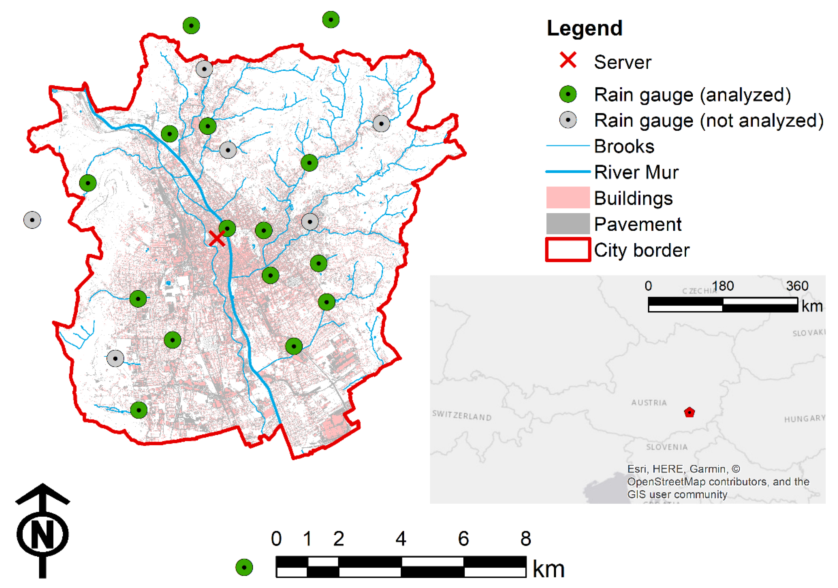
The data for this study is from Graz, a city in the south east of Austria at the southeastern outskirts of the Alps (see Figure 1). The city’s area is 125 km2 from which 33% is built-up area. Due to its location towards the Alps, the city is mostly shielded from the prevailing westerly winds bringing in weather fronts from the North Atlantic. The climate is classified as a humid continental climate with influences from the Mediterranean climate because it lies in a basin that is only open to the south, which makes it susceptible to low-pressure areas from the Mediterranean [47]. The average annual precipitation for the study site is 860 mm, 70% of which occurs throughout April to September (with 40–50 storm days), which we will refer to as the warm period for the rest of this paper. Most severe storms can be categorized as convective summer storms and are the main challenge for local infrastructure management. Their highly localized storm cells can cause severe flash floods and overcharge the combined sewer system of the city center. Further, combined sewer overflows happen on a regular basis due to these storms. The eastern part of the city is interspersed by multiple brooks draining large catchments that can potentially flood parts of the city as well. Retention basins as well as linear flow mitigation measures have been built along the brooks over the course of the last decade to defuse the fluvial flooding situation. Together with these measures, rain gauges and flow measurement stations were set up as well.
3. Data and Methods
3.1. Data
In 2014, all the organizations running high-quality rain gauges in the city of Graz decided to combine and share their measurement data as well as intensify the measurement density for the city. This led to the foundation of the Graz City Measurement Network (GCMN—Table 2 and Figure 1). The oldest rain gauge included in the network was installed in 1994 and 3 more were set up by 2014. Only after the foundation of the GCMN, rain gauges were (and still are) added much faster than in the years before. Today, the GCMN runs 22 rain gauges that are collecting online precipitation data for the city’s area of 125 km2. Twenty-one rain gauges are weighing precipitation gauges (19 OTT HydroMet—Pluvio2, 2 MPS systém—TRWS504 and TRWS503) and one is a tipping bucket rain gauge (Paar AP23). They are all operating with a temporal resolution of one minute or higher and a volumetric accuracy of at least 0.1 mm. Three rain gauges are not heated and therefore do not measure solid precipitation during periods of low temperatures. Each rain gauge uses GSM to send its data to a central server and to synchronize their time stamps regularly.
The rain gauges send their data to a server at the fire department of Graz. Via FTP, the data is then transferred to the other project partners in near real-time. This way the data is fully available at decentralized locations in case of a server failure.
3.2. Data Analysis
The data analyzed in this paper are the validated precipitation time series from 19 out of 22 rain gauges from the years 2017 and 2018 (network size at that time). Three rain gauges either had known defects during that time or showed too many data inconsistencies during the validation process. Therefore, those three rain gauges had to be ignored in the analyses of this paper along with the three rain gauges that were not set up at the time (gray rain gauges in Figure 1). In order to get comparable events, the time series went through an event detection algorithm as used in Leimgruber et al. [50]. The detection separated events with a minimum peak intensity of 2 mm/h and a minimum event gap of four hours. The event detection algorithm was applied to each individual time series as well as to the sum of all time series. The sum was then used to generate citywide events for an event-wise comparison.
Initially, we looked at all events for correlations of all rain gauges to each other in relation to rainfall intensity, event sum, event duration, interstation distance, seasonal differences and event peak occurrence. Subsequently, the event sums of all rain gauges were plotted against each other in sum comparison plots. This happened for all events to see if there are general correlations between the rain gauges. Each parameter was grouped by magnitudes to find common behaviors or classes for events. The parameters showing the most effects were then further investigated.
Following this, we looked at the interpolated rainfall of storms for the entire city. To do that, a grid consisting of 6200 squares, each with a size of 150 × 150 m to resemble the most likely pixel size of an x-band radar system, was generated that covers the entire city. All spatial interpolations use this sample grid in order to generate spatially distributed rainfall. To reduce the number of interpolations only relevant events were analyzed in this regard. After performing various analyses on the existing data including visual inspections of spatial interpolations of event rainfalls as well as using our experience with the study site, we chose the following selecting criteria for the events for this analysis:
- The arithmetic mean of the event rainfall of all rain gauges for the selected events was at least 15 mm.
- Rainfall had to be measured at least at 10 rain gauges during the event
These criteria resulted in a manageable collection of events with a wide range of event intensities that provide a good sample of the precipitation characteristics of the study site.
To account for spatial variability, an algorithm based on the inverse distance method introduced by Shepard [51] was used with the sample grid from above. The algorithm interpolates the rainfall from various combinations of rain gauges created with a variable number of rain gauges and then calculates the arithmetic mean of the interpolated grid for all combinations. This creates mean event rainfalls factoring in the spatial variability of the events. The amount of all possible combinations calculates as follows:
with:
n = number of all available rain gauges
k = number of rain gauges used to generate combinations
n ranges from 1 to all available rain gauges for the current event with all combinations that fulfill a diversity criterion. The criterion prohibits combinations e.g., of two rain gauges in the same area of the city from generating an interpolation over the whole city. The criterion means to reflect common sense in setting up a measurement network and at the same time limits the number of combinations to a manageable size. The diversity criterion for each combination within a number of rain gauges is as follows:
with:
x = number of all possible paths between rain gauges for the current combination
di = distance between 2 rain gauges
dall = mean of all distances between all available rain gauges
Each valid combination yields an interpolated rainfall for the city for each event. The results were then separated by the sample size used, to create the interpolation. The interpolation with the maximum available number of rain gauges is the most accurate result possible and therefore the reference for all other results, which are expressed as deviations from it. Combining the combinations of each number of rain gauges to boxplots shows the introduced deviation from the best result when using a smaller number of rain gauges than available. These analyses are grouped by season and by their maximum hourly intensity measured during the event to point out seasonal differences as well as the severity of spatial variability for different rainfall intensities.
4. Results and Discussion
As already described in data analysis in the methodology section 16 out of 22 available rain gauges were used for the analyzed period of the years 2017 and 2018. With the exception of one of the analyzed rain gauges with a gap of 10 days in August 2017, there were no other inconsistencies after the validation process.
The event detection resulted in 147 events meeting the criteria of the citywide event detection algorithm. There were 24 events that met the criteria of relevant events for further analysis. The 24 events are listed in Table 4 along with some key characteristics of the events. Only four of them occurred during the cold period of the year and hence, are bold in Table 4. None of them fell in the above-mentioned gap.
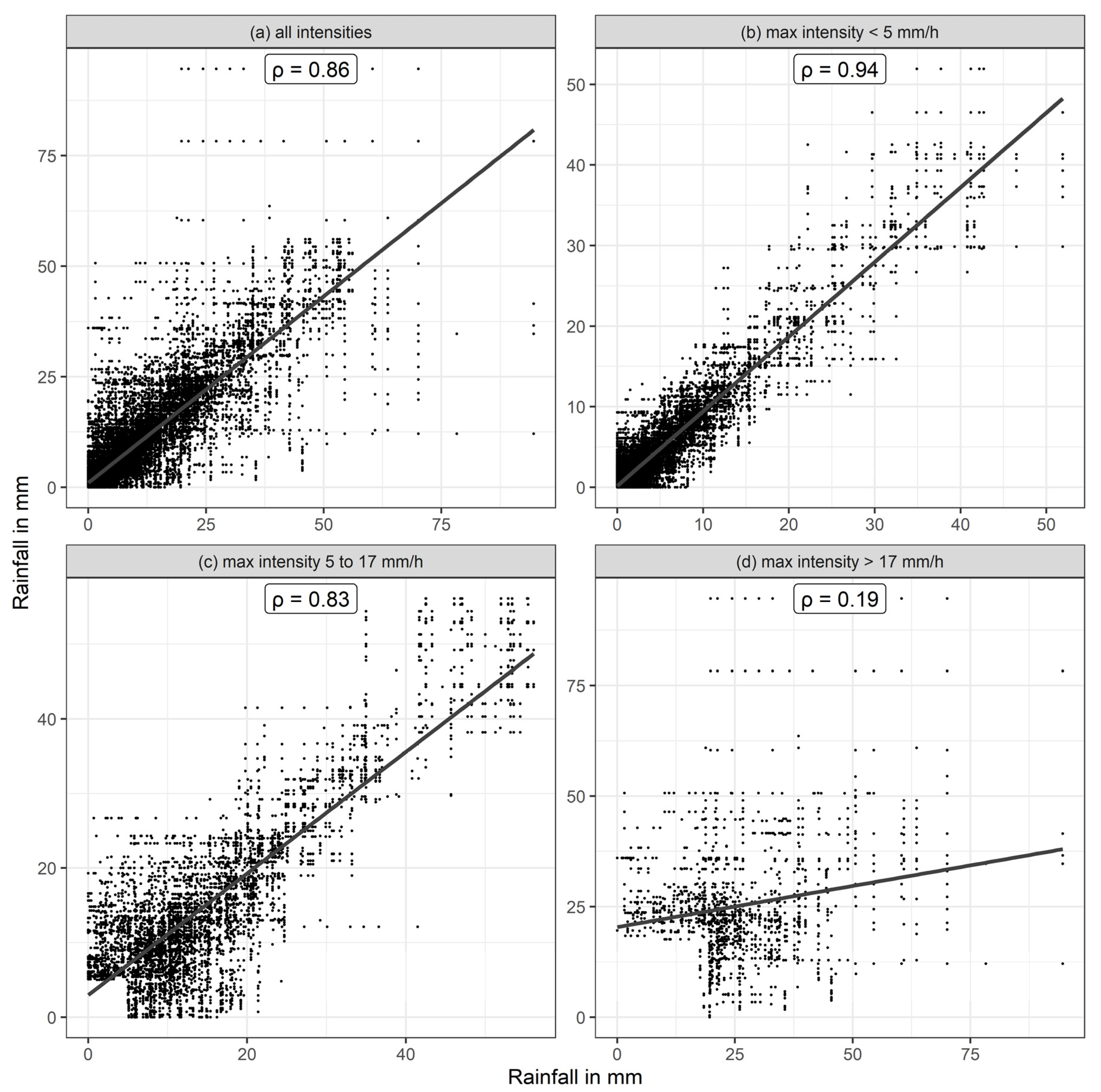
The event-wise comparison of the event sums of every rain gauge with each other reveals a good linear correlation with a Pearson correlation coefficient of 0.86 as plotted in Figure 2a, where in addition to the correlation coefficient a sum comparison plot together with its linear regression is shown. The events were classified by their overall mean of the maximum hourly intensities in Figure 2b–d. From our experience with the study site we know that events with maximum intensities lower than 5 mm/h usually don’t generate significant enough runoff to pose any problems for the urban water management which is why they were grouped together in Figure 2b. The classification between Figure 2c,d was introduced to separate heavy rainfall events with hourly intensities higher than 17 mm/h after the criterion by Wussow (as described in Maniak [52]) from less intense rainfall events. We find good interstation correlations for events up to 17 mm/h as depicted in Figure 2b,c with correlation coefficients of at least 0.83. However, the correlation coefficient drops down to only 0.19 for higher intensity rainfalls as shown in Figure 2d which suggests a much higher spatial variability for these heavy rainfall events.
Many of these events are convectional storms, which mainly occur throughout spring and summer. The results of Faurès et al. [30] and Goodrich et al. [31] who found that the assumption of spatial rainfall uniformity of convective rainfall is invalid support these findings. Considering that these high intensity events are the significant ones for most objectives in infrastructure management, this means that it is of high importance to measure these convective storms accurately enough to account for their significant spatial variability in urban environments.
Similar analyses were performed grouping the dataset by other intensities from five minutes up to two hours, the total event rainfall, interstation distance and event duration. Whereas those analyses showed similar results as mentioned above for other intensities (the strongest effect was found for 1 and 1.5 h intensities), correlation changes were neither very prominent for different total event rainfalls nor for event durations. So, similar to the findings of Villarini et al. [38] and Muthusamy et al. [32] the spatial variability decreases with decreasing temporal resolutions (12 hourly or daily rainfall). The only other factor showing a strongly decreasing correlation was the interstation distance. The further the rain gauges were apart from each other the worse their correlation was with each other, which shows the general spatial heterogeneity of all measured events.
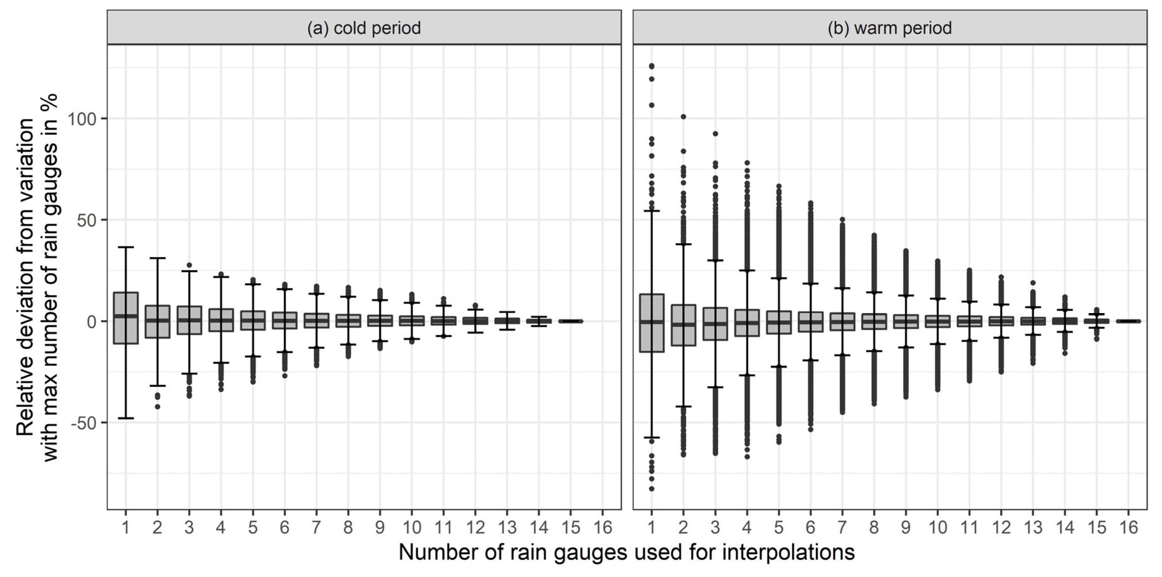
The measured event volumes of each rain gauge from the 24 events from Table 4 act as the sample from which the rainfall is interpolated over the catchment as explained earlier in the methods. The sample size ranges from 1 to 16 measurements for each event whereas each sample size also comprises all combinations with that size fulfilling the diversity criterion (mean interstation distance longer than 6 km). Therefore, per sample size we generated multiple mean event rainfalls. The mean event rainfall interpolated from the maximum available number of measurements of each event represents the most accurate result possible. All other results are expressed as relative deviations from it and are summarized in boxplots for each sample size in Figure 3 and Figure 4. With 16 rain gauges, this process generates 41,525 possible mean rainfalls for each event. The combination of the boxplots for all possible sample sizes shows the resulting ranges created by omitting available spatial information for the rainfall events.
Grouping the events into cold and warm periods as done in Figure 3 shows that the deviation converges faster towards the best interpolation for the events in the cold period (see Figure 3a). Keeping in mind that only four events from the cold period met the criteria for this analysis (none of them having all 16 rain gauges recording precipitation during the same event) shows that events during the warm period tend to have a higher spatial variability (Figure 3b). This effect can already be seen in the inner two quartiles. However, the whiskers and outliers show the full extent of the possible deviation induced by omitting available measurements. Representing the more unfortunate measurement combinations for each event, they show that omitting just one measurement during the summer period can result in a deviation of more than 5%. Using half the measurements available leads to a deviation of up to 40%, and only utilizing the information of a single rain gauge can increase the deviation to 125% for the warm period in a worst-case scenario. These results concur with Bárdossy and Das [42] who also found larger spatial rainfall variability throughout the summer months that majorly impacted their model performance when reducing the number of measurements as input for a semi-distributed hydrological model. They concluded that convective rainstorms mainly occur during the summer for their study, which is also the case for the study site of this paper.
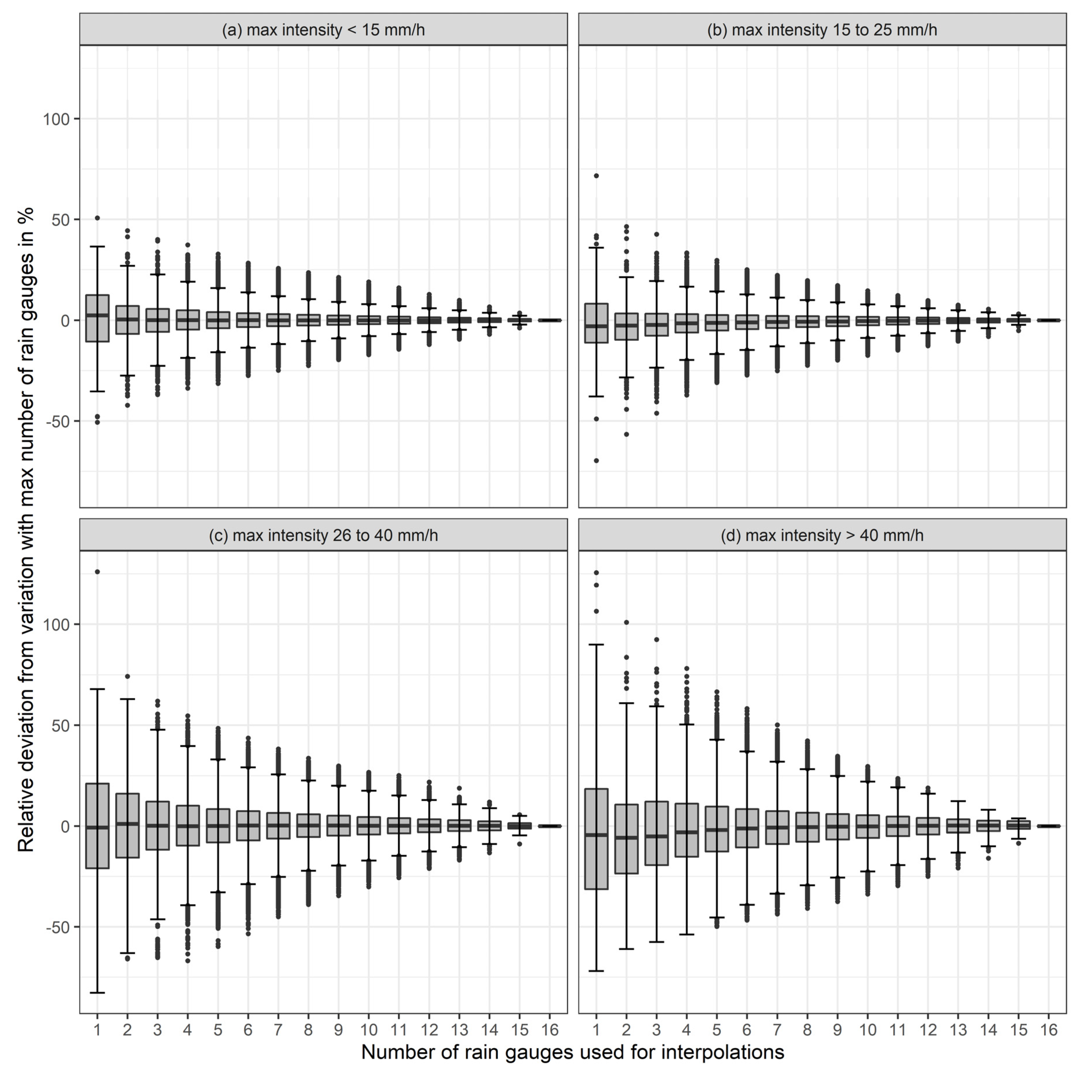
When grouping the events by the maximum measured hourly intensity of any rain gauge of each event as done in Figure 4 into four equally sized groups of events, it is apparent that more intense events show a much higher spatial variability than the less intense ones. This is supported by the results of Girons Lopez et al. [43] who came to the same conclusion. This does not mean that the deviation is negligible for events with smaller intensities than 26 mm/h (see Figure 4a,b). For these smaller events the deviation still goes up to 25% when using half the available measurements and up to 75% when using a single measurement.
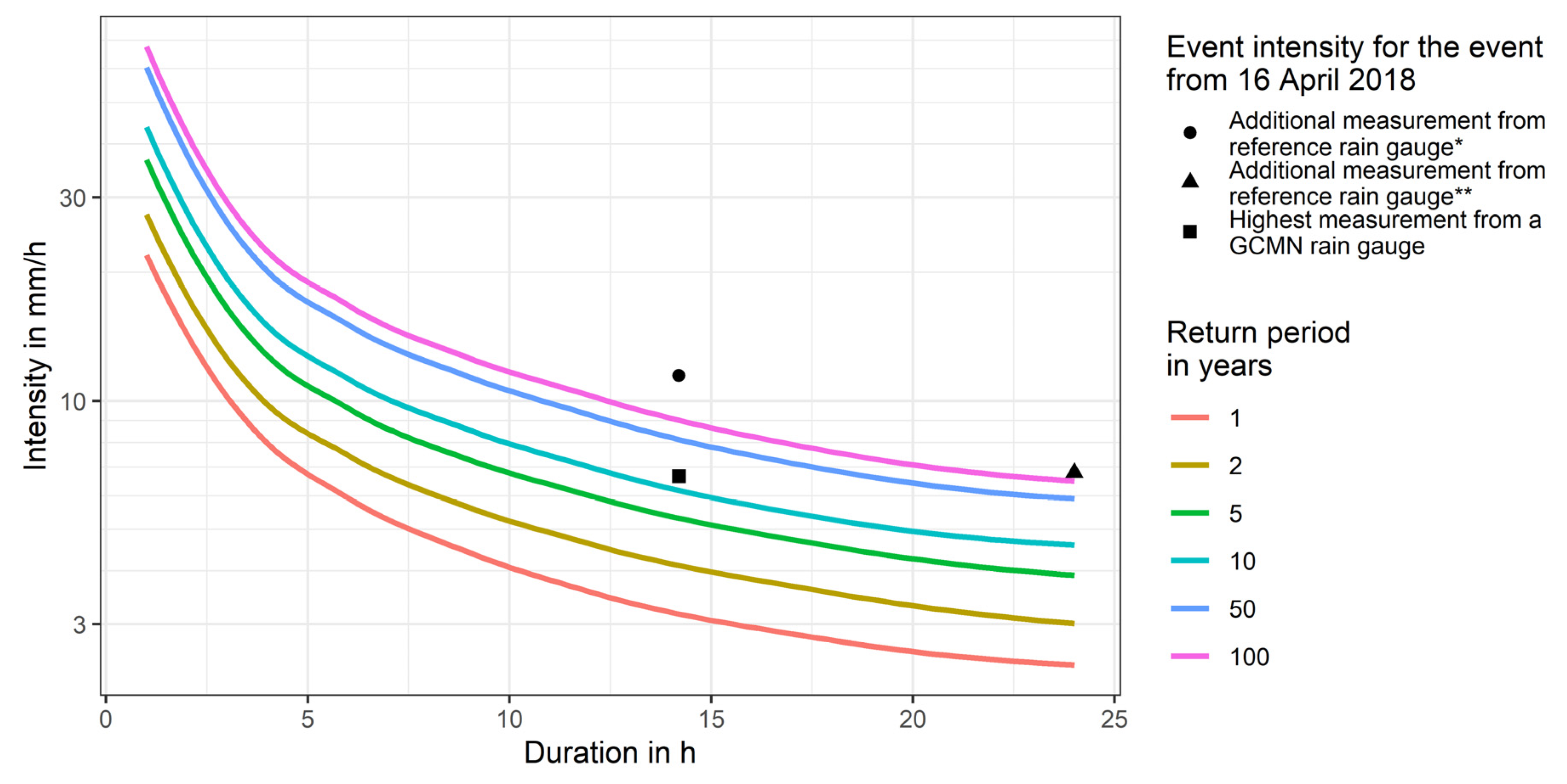
However, events with intensities of 26 mm/h and higher show much bigger deviations (Figure 4c,d). Using eight measurements for the interpolation results in deviations up to 45% versus 125% using single measurements. This is particularly important because these intensities include return periods of one to five years (see Figure 4c) and longer (see Figure 4d), which are significant for several design processes for urban infrastructure like the sewer system hydraulics or urban flood mitigation measures. So, contrary to the findings of Peleg et al. [46] return periods shorter than five years do benefit from a very high measurement density. Nevertheless, the effect does intensify even more for longer return periods. For relevant return periods for the location of the dataset’s origin, see Figure 5. The shown intensity-duration-frequency (IDF) curves are based on extreme value predictions from the Styrian Federal State Department for Hydrographical Observations who used the time series of the oldest rain gauge of the GCMN set up in 1994, as well as historical data starting in 1891 for the same location [53].
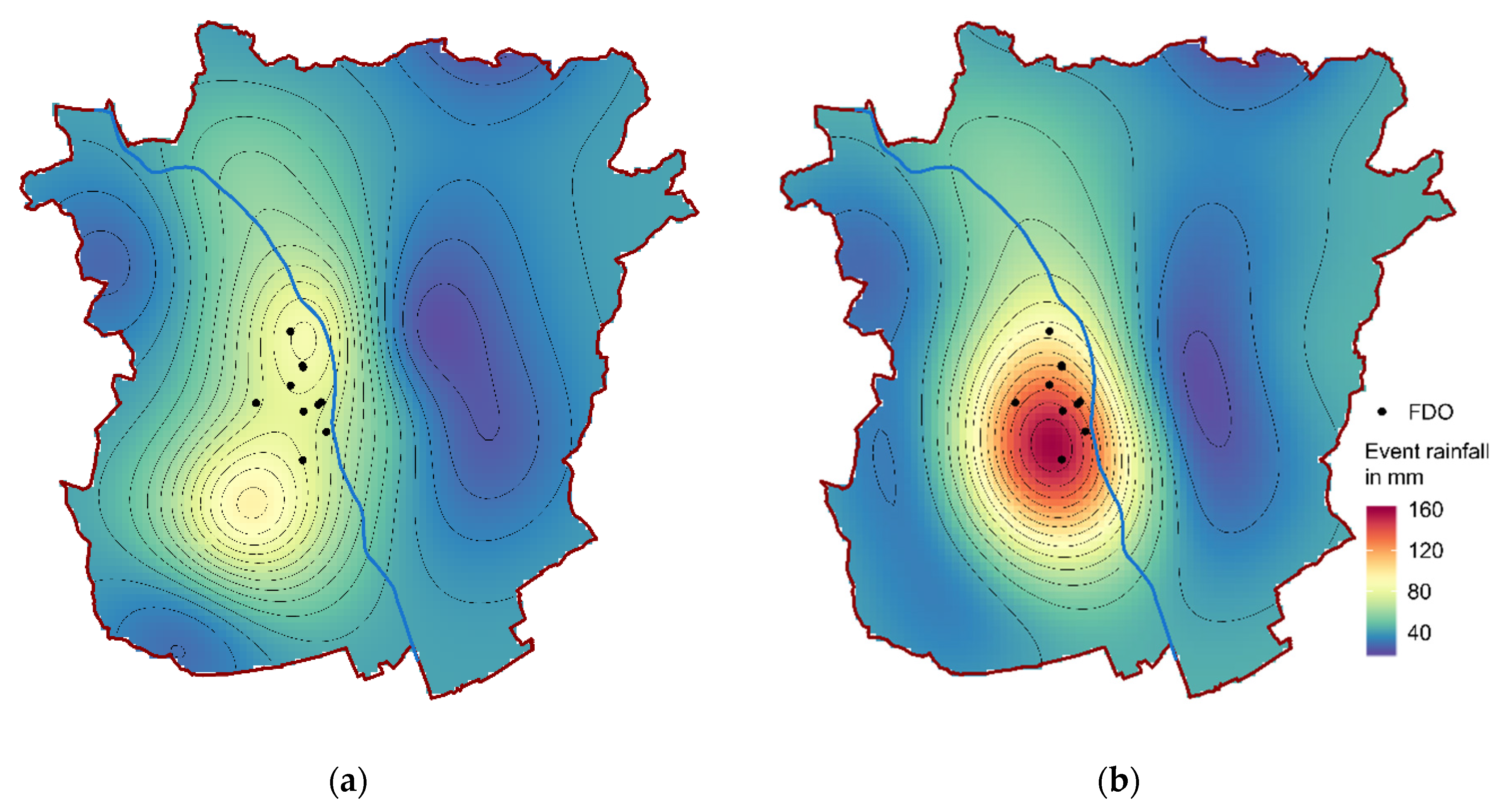
The event from 16 April 2018 stands out from the rest of the chosen events. It had the second highest hourly intensity of 52 mm/h measured at a single rain gauge and the highest average event rainfall as well as the highest event rainfall measured at a single rain gauge (see Table 4). The return period of the event is 14.5 years for the entire event duration, which makes it particularly interesting for further analysis. An indicator for the actual location of the rainstorm’s center is the detailed information of the extent of the urban flooding available for this event comprised by local news reports, videos, and photographs, and the operation log of the city’s fire department. Figure 6 shows two different event rainfall interpolations of the event as well as the locations of urban flooding related operations of the city’s fire department of that event. Figure 6a uses the measurements of the 16 GCMN rain gauges as the sample for the interpolation. However, this areal precipitation does not fully explain the locations of the flooding. Therefore, the sample of the interpolation in Figure 6b contains an additional measurement of a validation rain gauge that only measures daily rainfall volumes and is usually not included in the GCMN. This rain gauge measured 163 mm for the event in comparison to 94.6 mm at the closest GCMN rain gauge only 1.4 km away, which puts the return period of the event above 100 years (as indicated in Figure 5). The local observations of severe and highly localized pluvial flooding of the area support the correctness of the additional measurement. This event shows that the current high-density measurement network with a measurement resolution of one rain gauge per 7.8 km2 (using 16 gauges) is still insufficient to capture the spatial variability of convectional high-intensity rainfall events.
These findings agree with the original recommendation of Schilling [45], who offered a ‘guesstimate’ of a necessary spatial measurement resolution of one rain gage per 1 km2 and Berne et al. [16], who, while limiting their recommendation to catchments of the order of 1000 ha, suggest 1 rain gauge per 3 km2.
Findings of other groups researching the spatial variability of rainfall on a sub-kilometer scale [33,35,36,37] show that the spatial variability on such a small scale can go as high as 100% within one square kilometer. The results shown in Figure 6, however, are the first that show the severity of this effect for an urban environment.
5. Conclusions
A high-density precipitation measurement network for a city in a humid continental climate was introduced in this paper. The measurements from 16 out of currently 22 rain gauges from the years 2017 and 2018 were used to show the importance of spatial rainfall variability and the benefits of a high-density rain gauge network. We found that the overall correlation between the rain gauges of a large urbanized catchment is good for small and intermediate rainfall events. However, the higher the rainfall intensities are, the lower is the interstation correlation. This is particularly significant for heavy rainfall events with intensities above 17 mm/h. This suggests that multiple rain gauges are necessary to feasibly measure rainfall over a larger catchment.
By using the available high measurement density of the study site as a reference for the best possible measurement result for the spatial variability of 24 chosen rainfall events, we showed how reducing the measurement density affects the spatially interpolated event rainfall. Using eight instead of 16 rain gauges to interpolate the resulting event rainfalls results in deviations of up to 25% for smaller rainfall events and up to 45% for events with return periods of one or more years. Assuming uniformly distributed rainfall by using only the measurements of a single rain gauge results in deviations of up to 75% and 125%, respectively. Storms with intensities that high usually only occur during spring or summer months and follow a convectional rainfall pattern as opposed to lower intensity frontal rainfall events throughout the fall and winter months.
Considering that storms with return periods of one year and longer are essential for the design processes of most urban infrastructure, this shows that ignoring the spatial rainfall variability of storms for the input of rainfall runoff models can falsify simulation results significantly. High-detailed models with a short catchment response would especially suffer from too little spatial information.
To quantify the full extent of this problem, further research is necessary, which pairs the results from this paper with hydrological and hydraulic models. The results of different modeling objectives might be affected to other degrees, depending on the processes involved.
With much research already done in rural landscapes with higher measurement resolutions than the one used in this paper it is clear that the current measurement resolution of one rain gauge per 6 km2 (all 22 rain gauges) is not sufficient to fully account for the spatial variability of convective summer storms. Additional data from e.g., remote sensing technologies could supplement the current dataset for future research. Nevertheless, it was clearly shown that the current common practice of assuming uniform rainfall for an urban environment leads to significant errors and is not recommendable for any kind of simulation.
Author Contributions
Conceptualization, R.M., G.K. and D.M.; methodology, R.M.; software, R.M. and M.P.; validation, R.M. and M.P.; formal analysis, R.M.; investigation, R.M.; resources, R.M. and G.G.; data curation, R.M., M.P. and G.G.; writing—original draft preparation, R.M.; writing—review and editing, R.M., G.K., M.P., D.M. and G.G.; visualization, R.M.; supervision, D.M.; project administration, G.G.; funding acquisition, D.M. All authors have read and agree to the published version of the manuscript.
Funding
Open Access Funding by the Graz University of Technology.
Acknowledgments
We would like to thank all the participants of the Graz City Measurement Network for sharing their data.
Conflicts of Interest
The authors declare no conflict of interest.
References
- James, W. Rules for Responsible Modelling; CHI—Computational Hydraulics International: Guelph, ON, Canada, 2005. [Google Scholar]
- Jacobson, C.R. Identification and quantification of the hydrological impacts of imperviousness in urban catchments: A review. J. Environ. Manag. 2011, 92, 1438–1448. [Google Scholar] [CrossRef] [PubMed]
- Deletic, A.; Dotto, C.B.S.; McCarthy, D.T.; Kleidorfer, M.; Freni, G.; Mannina, G.; Uhl, M.; Henrichs, M.; Fletcher, T.D.; Rauch, W.; et al. Assessing uncertainties in urban drainage models. Phys. Chem. Earth 2012, 42–44, 3–10. [Google Scholar] [CrossRef] [Green Version]
- Chen, Y.; Zhou, H.; Zhang, H.; Du, G.; Zhou, J. Urban flood risk warning under rapid urbanization. Environ. Res. 2015, 139, 3–10. [Google Scholar] [CrossRef] [PubMed]
- Salvadore, E.; Bronders, J.; Batelaan, O. Hydrological modelling of urbanized catchments: A review and future directions. J. Hydrol. 2015, 529 Pt 1, 62–81. [Google Scholar] [CrossRef]
- Cristiano, E.; ten Veldhuis, M.-C.; van de Giesen, N. Spatial and temporal variability of rainfall and their effects on hydrological response in urban areas—A review. Hydrol. Earth Syst. Sci. 2017, 21, 3859–3878. [Google Scholar] [CrossRef] [Green Version]
- Shepherd, J.M. A Review of Current Investigations of Urban-Induced Rainfall and Recommendations for the Future. Earth Interact. 2005, 9, 1–27. [Google Scholar] [CrossRef] [Green Version]
- Ly, S.; Charles, C.; Degre, A. Geostatistical interpolation of daily rainfall at catchment scale: The use of several variogram models in the Ourthe and Ambleve catchments, Belgium. Hydrol. Earth Syst. Sci. 2011, 15, 2259–2274. [Google Scholar] [CrossRef] [Green Version]
- Wagner, P.D.; Fiener, P.; Wilken, F.; Kumar, S.; Schneider, K. Comparison and evaluation of spatial interpolation schemes for daily rainfall in data scarce regions. J. Hydrol. 2012, 464–465, 388–400. [Google Scholar] [CrossRef]
- Sungmin, O.; Foelsche, U.; Kirchengast, G.; Fuchsberger, J. Validation and correction of rainfall data from the WegenerNet high density network in southeast Austria. J. Hydrol. 2018, 556, 1110–1122. [Google Scholar]
- De Vos, L.W.; Leijnse, H.; Overeem, A.; Uijlenhoet, R. Quality Control for Crowdsourced Personal Weather Stations to Enable Operational Rainfall Monitoring. Geophys. Res. Lett. 2019, 46, 8820–8829. [Google Scholar] [CrossRef] [Green Version]
- Bárdossy, A.; Seidel, J.; Hachem, A.E. The use of personal weather station observation for improving precipitation estimation and interpolation. Hydrol. Earth Syst. Sci. Discuss. 2020, 1–23. [Google Scholar] [CrossRef] [Green Version]
- Krajewski, W.F.; Villarini, G.; Smith, J.A. RADAR-Rainfall Uncertainties. Bull. Am. Meteorol. Soc. 2010, 91, 87–94. [Google Scholar] [CrossRef]
- Villarini, G.; Krajewski, W.F. Review of the different sources of uncertainty in single polarization radar-based estimates of rainfall. Surv. Geophys. 2010, 31, 107–129. [Google Scholar] [CrossRef]
- Sharifi, E.; Steinacker, R.; Saghafian, B. Assessment of GPM-IMERG and other precipitation products against gauge data under different topographic and climatic conditions in Iran: Preliminary results. Remote Sens. 2016, 8, 135. [Google Scholar] [CrossRef] [Green Version]
- Berne, A.; Delrieu, G.; Creutin, J.-D.; Obled, C. Temporal and spatial resolution of rainfall measurements required for urban hydrology. J. Hydrol. 2004, 299, 166–179. [Google Scholar] [CrossRef]
- Gires, A.; Onof, C.; Maksimovic, C.; Schertzer, D.; Tchiguirinskaia, I.; Simoes, N. Quantifying the impact of small scale unmeasured rainfall variability on urban runoff through multifractal downscaling: A case study. J. Hydrol. 2012, 442–443, 117–128. [Google Scholar] [CrossRef] [Green Version]
- Gires, A.; Giangola-Murzyn, A.; Abbes, J.-B.; Tchiguirinskaia, I.; Schertzer, D.; Lovejoy, S. Impacts of small scale rainfall variability in urban areas: A case study with 1D and 1D/2D hydrological models in a multifractal framework. Urban Water J. 2015, 12, 607–617. [Google Scholar] [CrossRef] [Green Version]
- Ochoa-Rodriguez, S.; Wang, L.-P.; Gires, A.; Pina, R.D.; Reinoso-Rondinel, R.; Bruni, G.; Ichiba, A.; Gaitan, S.; Cristiano, E.; Van, A.; et al. Impact of spatial and temporal resolution of rainfall inputs on urban hydrodynamic modelling outputs: A multi-catchment investigation. J. Hydrol. 2015, 531, 389–407. [Google Scholar] [CrossRef]
- Steiner, M.; Smith, J.A.; Burges, S.J.; Alonso, C.V.; Darden, R.W. Effect of bias adjustment and rain gauge data quality control on radar rainfall estimation. Water Resour. Res. 1999, 35, 2487–2503. [Google Scholar] [CrossRef]
- Borga, M.; Tonelli, F.; Moore, R.J.; Andrieu, H. Long-term assessment of bias adjustment in radar rainfall estimation. Water Resour. Res. 2002, 38, 8-1–8-10. [Google Scholar] [CrossRef] [Green Version]
- Matrosov, S.Y.; Kingsmill, D.E.; Martner, B.E.; Ralph, F.M. The Utility of X-Band polarimetric radar for quantitative estimates of rainfall parameters. J. Hydrometeorol. 2005, 6, 248–262. [Google Scholar] [CrossRef] [Green Version]
- Schleiss, M.; Olsson, J.; Berg, P.; Niemi, T.; Kokkonen, T.; Thorndahl, S.; Nielsen, R.; Nielsen, J.E.; Bozhinova, D.; Pulkkinen, S. The accuracy of weather radar in heavy rain: A comparative study for Denmark, the Netherlands, Finland and Sweden. Hydrol. Earth Syst. Sci. Discuss. 2019. in review. [Google Scholar] [CrossRef] [Green Version]
- Aalborg (DK)—MUFFIN. Available online: https://muffin-project.eu/aalborg-dk/ (accessed on 26 February 2020).
- Landsberg, H.E. Man-made climatic changes. Science 1970, 170, 1265–1274. [Google Scholar] [CrossRef] [PubMed]
- Smith, C.; Levermore, G. Designing urban spaces and buildings to improve sustainability and quality of life in a warmer world. Energy Policy 2008, 36, 4558–4562. [Google Scholar] [CrossRef]
- Sevruk, B. Rainfall Measurement: Gauges. In Encyclopedia of Hydrological Sciences; American Cancer Society: New York, NY, USA, 2006; ISBN 978-0-470-84894-4. [Google Scholar]
- AghaKouchak, A.; Mehran, A.; Norouzi, H.; Behrangi, A. Systematic and random error components in satellite precipitation data sets. Geophys. Res. Lett. 2012, 39, 9406. [Google Scholar] [CrossRef] [Green Version]
- Kirstetter, P.-E.; Hong, Y.; Gourley, J.J.; Chen, S.; Flamig, Z.; Zhang, J.; Schwaller, M.; Petersen, W.; Amitai, E. Toward a framework for systematic error modeling of spaceborne precipitation radar with NOAA/NSSL ground radar–based national mosaic QPE. J. Hydrometeorol. 2012, 13, 1285–1300. [Google Scholar] [CrossRef]
- Faurès, J.-M.; Goodrich, D.C.; Woolhiser, D.A.; Sorooshian, S. Impact of small-scale spatial rainfall variability on runoff modeling. J. Hydrol. 1995, 173, 309–326. [Google Scholar] [CrossRef]
- Goodrich, D.C.; Faurès, J.-M.; Woolhiser, D.A.; Lane, L.J.; Sorooshian, S. Measurement and analysis of small-scale convective storm rainfall variability. J. Hydrol. 1995, 173, 283–308. [Google Scholar] [CrossRef]
- Muthusamy, M.; Schellart, A.; Tait, S.; Heuvelink, G.B.M. Geostatistical upscaling of rain gauge data to support uncertainty analysis of lumped urban hydrological models. Hydrol. Earth Syst. Sci. 2017, 21, 1077–1091. [Google Scholar] [CrossRef] [Green Version]
- Jensen, N.E.; Pedersen, L. Spatial variability of rainfall: Variations within a single radar pixel. Atmos. Res. 2005, 77, 269–277. [Google Scholar] [CrossRef]
- Pedersen, L.; Jensen, N.E.; Christensen, L.E.; Madsen, H. Quantification of the spatial variability of rainfall based on a dense network of rain gauges. Atmos. Res. 2010, 95, 441–454. [Google Scholar] [CrossRef]
- Fiener, P.; Auerswald, K. Spatial variability of rainfall on a sub-kilometre scale. Earth Surf. Process. Landf. 2009, 34, 848–859. [Google Scholar] [CrossRef] [Green Version]
- Peleg, N.; Ben-Asher, M.; Morin, E. Radar subpixel-scale rainfall variability and uncertainty: Lessons learned from observations of a dense rain-gauge network. Hydrol. Earth Syst. Sci. 2013, 17, 2195–2208. [Google Scholar] [CrossRef] [Green Version]
- Ciach, G.J.; Krajewski, W.F. Analysis and modeling of spatial correlation structure in small-scale rainfall in Central Oklahoma. Adv. Water Resour. 2006, 29, 1450–1463. [Google Scholar] [CrossRef]
- Villarini, G.; Mandapaka, P.V.; Krajewski, W.F.; Moore, R.J. Rainfall and sampling uncertainties: A rain gauge perspective. J. Geophys. Res. Atmos. 2008, 113, D11102. [Google Scholar] [CrossRef]
- Bell, V.A.; Moore, R.J. The sensitivity of catchment runoff models to rainfall data at different spatial scales. Hydrol. Earth Syst. Sci. Discuss. 2000, 4, 653–667. [Google Scholar] [CrossRef]
- Zawilski, M.; Brzezińska, A. Areal rainfall intensity distribution over an urban area and its effect on a combined sewerage system. Urban Water J. 2014, 11, 532–542. [Google Scholar] [CrossRef]
- Arnaud, P.; Bouvier, C.; Cisneros, L.; Dominguez, R. Influence of rainfall spatial variability on flood prediction. J. Hydrol. 2002, 260, 216–230. [Google Scholar] [CrossRef]
- Bárdossy, A.; Das, T. Influence of rainfall observation network on model calibration and application. Hydrol. Earth Syst. Sci. Discuss. 2006, 3, 3691–3726. [Google Scholar] [CrossRef]
- Girons Lopez, M.; Wennerström, H.; Nordén, L.-Å.; Seibert, J. Location and Density of Rain Gauges for the Estimation of Spatial Varying Precipitation. Geogr. Ann. Ser. Phys. Geogr. 2015, 97, 167–179. [Google Scholar] [CrossRef] [Green Version]
- Berndtsson, R.; Niemczynowicz, J. Spatial and temporal scales in rainfall analysis—Some aspects and future perspectives. J. Hydrol. 1988, 100, 293–313. [Google Scholar] [CrossRef]
- Schilling, W. Rainfall data for urban hydrology: What do we need? Atmos. Res. 1991, 27, 5–21. [Google Scholar] [CrossRef]
- Peleg, N.; Blumensaat, F.; Molnar, P.; Fatichi, S.; Burlando, P. Partitioning the impacts of spatial and climatological rainfall variability in urban drainage modeling. Hydrol. Earth Syst. Sci. 2017, 21, 1559–1572. [Google Scholar] [CrossRef] [Green Version]
- Belda, M.; Holtanová, E.; Halenka, T.; Kalvová, J. Climate classification revisited: From Köppen to Trewartha. Clim. Res. 2014, 59, 1–13. [Google Scholar] [CrossRef] [Green Version]
- Kabas, T.; Leuprecht, A.; Bichler, C.; Kirchengast, G. WegenerNet climate station network region Feldbach, Austria: Network structure, processing system, and example results. Adv. Sci. Res. 2011, 6, 49–54. [Google Scholar] [CrossRef] [Green Version]
- Kirchengast, G.; Kabas, T.; Leuprecht, A.; Bichler, C.; Truhetz, H. WegenerNet: A pioneering high-resolution network for monitoring weather and climate. Bull. Am. Meteorol. Soc. 2013, 95, 227–242. [Google Scholar] [CrossRef]
- Leimgruber, J.; Steffelbauer, D.B.; Krebs, G.; Tscheikner-Gratl, F.; Muschalla, D. Selecting a series of storm events for a model-based assessment of combined sewer overflows. Urban Water J. 2018, 15, 453–460. [Google Scholar] [CrossRef]
- Shepard, D. A two-dimensional interpolation function for irregularly-spaced data. In Proceedings of the 1968 23rd ACM National Conference, Las Vegas, NV, USA, 27–29 August 1968; ACM: New York City, NY, USA, 1968; pp. 517–524. [Google Scholar]
- Maniak, U. Hydrologie und Wasserwirtschaft: Eine Einführung für Ingenieure; Lehrbuch; 7., neu bearbeitete Auflage.; Springer Vieweg: Berlin, Germany, 2016; ISBN 978-3-662-49087-7. [Google Scholar]
- eHYD—Access to the Hydrographical Data of Austira—Design Storm grid Point 5214. Available online: https://ehyd.gv.at/# (accessed on 4 March 2020).
Figure 1.
Locations of the rain gauges of the Graz City Measurement Network differentiated in rain gauges analyzed and not analyzed in this paper (owners listed in Table 2). The city’s location within Central Europe is indicated in the grey map.
Figure 1.
Locations of the rain gauges of the Graz City Measurement Network differentiated in rain gauges analyzed and not analyzed in this paper (owners listed in Table 2). The city’s location within Central Europe is indicated in the grey map.

Figure 2.
Rain gauge to rain gauge sum comparison plots of event rainfalls in mm with the calculated Pearson coefficient (ρ) and the linear regression in each subplot: (a) all intensities together in one plot; (b) small intensities <5 mm/h; (c) medium intensities between 5 and 17 mm/h; and (d) high intensity storms > 17 mm/h.

Figure 3.
Relative deviations of the mean rainfalls (calculated from spatial interpolations of rainfall events) from the mean rainfall calculated from the spatial interpolation with the highest rain gauge density (all available rain gauges used as sample size). The mean rainfalls are shown as boxplots grouped by the used sample size for the spatial interpolation of the event rainfall: (a) cold period = fall and winter and (b) warm period = spring and summer.

Figure 4.
Relative deviations of the mean rainfalls (calculated from spatial interpolations of rainfall events) from the mean rainfall calculated from the spatial interpolation with the highest rain gauge density (all available rain gauges used as sample size). The mean rainfalls are shown as boxplots grouped by the used sample size for the spatial interpolation of the event rainfall. (a–d) are equally sized groups of events grouped by their maximum hourly intensity measured during each event.

Figure 5.
Relevant intensity-duration-frequency (IDF) curves for infrastructure management and design processes for the location of the dataset’s origin (data from Styrian Federal State Department for Hydrographical Observations [53]). * assuming the event duration of 14.2 h evaluated from the 16 rain gauges from the GCMN; ** using the measured daily intensity.

Figure 6.
Interpolation of the storm from 16 April 2018 with a return period of 100+ years. The flooding locations are indicated by the logged flood related fire department operations (FDO): (a) with the rain gauges currently in the GCMN; (b) with the added information from a standard rain gauge used for daily reference values


Table 1.
Test catchments with high densities of rain gauges investigating spatial rainfall variability.
Table 1.
Test catchments with high densities of rain gauges investigating spatial rainfall variability.
| Source | Number of Gauges | Catchment Size | Area/Gauge | Type |
|---|---|---|---|---|
| Faurès et al. [30], Goodrich et al. [31] | 10 | <0.05 km2 | 0.005 km2 | rural |
| Muthusamy et al. [32] | 8 | 0.08 km2 | 0.01 km2 | urban |
| Jensen and Pedersen [33], Pedersen et al. [34] | 9 | 0.25 km2 | 0.03 km2 | rural |
| Fiener and Auerswald [35] | 13 | 1.4 km2 | 0.11 km2 | rural |
| Peleg et al. [36] | 14 | 4 km2 | 0.14 km2 | rural |
| Ciach and Krajewski [37] | 25 | 9 km2 | 0.36 km2 | rural |
| Villarini et al. [38], Bell and Moore [39] | 49 | 135 km2 | 2.8 km2 | rural |
| Berne et al. [16] | 25 | 300 km2 | 12 km2 | urban |
| Zawilski and Brzezińska [40] | 21 | 256 km2 | 12 km2 | urban |
| Arnaud et al. [41] | 49 | 2500 km2 | 51 km2 | mixed |
| Bárdossy and Das [42] | 51 | 4000 km2 | 78 km2 | mixed |
| Girons Lopez et al. [43] | 60 | 6400 km2 | 107 km2 | mixed |
Table 2.
Assembly of the Graz City Measurement Network (GCMN).
| Organization | Number of Rain Gauges |
|---|---|
| City Department of Parks and Water Bodies | 11 |
| Styrian Federal State Department for Hydrographical Observations | 2 |
| Austrian Institute for Meteorology and Geodynamics | 3 |
| Holding Graz Water Management | 5 |
| Graz University of Technology | 1 |
| Fire Department of Graz | Server |
Table 3.
Data validation stages.
| Stage | Name | Short Explanation |
|---|---|---|
| 0 | Raw data | Original data from central server as received from the rain gauge; any deviation from this data is done on the fly. |
| 1 | Identification of known defects | Check for data during periods of known defects and maintenance |
| 2 | Device specific validation | Check against device specific measurement limits |
| 3 | Climatological boundaries | Data exceeding physical and local climatologic boundaries |
| 4 | Validation of temporal variability | Max. possible changes per time based on climatological limits |
| 5 | Intrastation validation | Consistency with other sensors of measurement station if available |
| 6 | Statistical validation | Check if data is within limits of the site specific data history |
| 7 | Interstation validation | Compare data with neighboring rain gauges (median-based comparison) |
| 8 | External reference | Compare data with other data sources available (e.g., additional rain gauges measuring daily values) |
Table 4.
Summary of the 24 events chosen for analysis with the arithmetic mean of all active rain gauges and the maximums of individual gauges per event. Bold events are in the group “cold period”.
Table 4.
Summary of the 24 events chosen for analysis with the arithmetic mean of all active rain gauges and the maximums of individual gauges per event. Bold events are in the group “cold period”.
| Date (Year/Month/Day) | Rain Gauges | Duration in Hours | Mean Sum in mm | Max Gauge Sum in mm | Max Mean Intensity in mm/h | Max Gauge Intensity in mm/h |
|---|---|---|---|---|---|---|
| 2017-02-05 | 15 | 23.3 | 23.0 | 29.9 | 3.8 | 4.6 |
| 2017-04-27 | 16 | 24.9 | 32.9 | 52.5 | 5.4 | 7.4 |
| 2017-05-22 | 16 | 5.9 | 26.8 | 40.0 | 9.4 | 26.5 |
| 2017-07-01 | 16 | 2.2 | 19.3 | 30.4 | 16.9 | 28.6 |
| 2017-07-23 | 16 | 6.3 | 21.3 | 51.6 | 8.9 | 17.4 |
| 2017-08-02 | 16 | 3.5 | 18.4 | 26.9 | 12.7 | 18.3 |
| 2017-08-19 | 16 | 18.2 | 26.8 | 31.9 | 10.3 | 14.1 |
| 2017-09-01 | 16 | 12.1 | 16.9 | 29.4 | 11.9 | 19.2 |
| 2017-11-05 | 14 | 22.5 | 17.7 | 22.6 | 2.7 | 3.3 |
| 2017-11-07 | 14 | 18.6 | 16.5 | 21.1 | 3.0 | 4.2 |
| 2018-04-16 | 16 | 14.2 | 43.1 | 94.6 | 19.6 | 52.0 |
| 2018-04-26 | 16 | 10.6 | 18.6 | 22.5 | 6.0 | 10.2 |
| 2018-05-12 | 16 | 2.9 | 18.3 | 42.8 | 13.5 | 28.5 |
| 2018-05-14 | 16 | 22.7 | 33.3 | 48.1 | 4.2 | 6.2 |
| 2018-06-02 | 15 | 5.0 | 24.0 | 50.7 | 16.9 | 43.0 |
| 2018-06-08 | 16 | 7.3 | 19.1 | 27.5 | 12.6 | 21.2 |
| 2018-06-13 | 16 | 7.3 | 38.2 | 63.6 | 32.0 | 54.6 |
| 2018-06-21 | 16 | 11.4 | 21.1 | 34.0 | 16.5 | 27.4 |
| 2018-07-05 | 16 | 14.3 | 17.1 | 24.7 | 4.4 | 6.5 |
| 2018-08-10 | 16 | 4.9 | 22.9 | 37.6 | 18.1 | 32.3 |
| 2018-09-01 | 16 | 6.3 | 20.2 | 41.6 | 12.1 | 18.6 |
| 2018-09-07 | 16 | 5.8 | 15.9 | 23.8 | 6.9 | 10.8 |
| 2018-09-14 | 16 | 4.5 | 23.5 | 44.7 | 19.6 | 40.1 |
| 2018-11-25 | 14 | 31.8 | 24.8 | 30.9 | 3.1 | 4.0 |
© 2020 by the authors. Licensee MDPI, Basel, Switzerland. This article is an open access article distributed under the terms and conditions of the Creative Commons Attribution (CC BY) license (http://creativecommons.org/licenses/by/4.0/).
Share and Cite
MDPI and ACS Style
Maier, R.; Krebs, G.; Pichler, M.; Muschalla, D.; Gruber, G. Spatial Rainfall Variability in Urban Environments—High-Density Precipitation Measurements on a City-Scale. Water 2020, 12, 1157. https://doi.org/10.3390/w12041157
AMA Style
Maier R, Krebs G, Pichler M, Muschalla D, Gruber G. Spatial Rainfall Variability in Urban Environments—High-Density Precipitation Measurements on a City-Scale. Water. 2020; 12(4):1157. https://doi.org/10.3390/w12041157
Chicago/Turabian StyleMaier, Roman, Gerald Krebs, Markus Pichler, Dirk Muschalla, and Günter Gruber. 2020. "Spatial Rainfall Variability in Urban Environments—High-Density Precipitation Measurements on a City-Scale" Water 12, no. 4: 1157. https://doi.org/10.3390/w12041157
Note that from the first issue of 2016, this journal uses article numbers instead of page numbers. See further details here.