Comparison of Statistical and Machine Learning Models for Pipe Failure Modeling in Water Distribution Networks

Abstract

The application of statistical and Machine Learning models plays a critical role in planning and decision support processes for efficient and reliable Water Distribution Network (WDN) management. Failure models can provide valuable information for prioritizing system rehabilitation even in data scarcity scenarios, such as developing countries. Few studies have analyzed the performance of more than two models, and examples of case studies in developing countries are insufficient. This study compares various statistical and Machine Learning models to provide useful information to practitioners for the selection of a suitable pipe failure model according to information availability and network characteristics. Three statistical models (i.e., Linear, Poisson, and Evolutionary Polynomial Regressions) were used for failure prediction in groups of pipes. Machine Learning approaches, particularly Gradient-Boosted Tree (GBT), Bayes, Support Vector Machines and Artificial Neuronal Networks (ANNs), were compared in predicting individual pipe failure rates. The proposed approach was applied to a WDN in Bogotá (Colombia). The statistical models showed an acceptable performance (R² between 0.695 and 0.927), but the Poisson Regression was the most suitable for predicting failures in pipes with lower failure rates. Regarding Machine Learning models, Bayes and ANNs exhibited low performance in the prediction of pipe failure condition. The GBT approach had the best performing classifier.

1. Introduction

The main purpose of Water Distribution Networks (WDNs) is to supply water to the population in the required quantity and quality [1]. Factors such as climate change, deterioration of system components, uncertainty regarding the physical condition of the pipes, growing water demand, and economic restrictions increase the complexity of their management [2]. A proper strategy for operation, maintenance, and rehabilitation of WDNs needs to be developed to ensure efficient and reliable management. Therefore, improving the efficiency in water supply and leakage reduction in WDNs should be strategic priorities for the sustainable development of water resources [3,4].

Pipe failures in WDNs may cause economic, environmental, and social costs resulting from water supply and traffic interruption, contaminant intrusion through the network, and loss of resources such as water and energy [5,6]. According to the United Nations, water utility assets in developing countries are more likely to be poorly managed due to inappropriate political administration and the increased pressure on the available water resources. Thus, the general lack of preventive maintenance plans has led to low-performing WDNs [7]. In Bogotá, Colombia’s capital city, the water loss rate ranges between 40% and 50% [8]. The WDNs renewal plans have focused on replacing asbestos-cement, galvanized iron, and ductile iron pipes with new plastic materials such as polyvinyl chloride (PVC). However, an adequate renewal prioritization strategy has not being implemented. Instead, a reactive strategy is adopted in which a pipe is rehabilitated or replaced after the failure is detected, implying low efficiency and poor service quality. The effective renovation planning of the WDNs requires, among other things, an accurate quantification of the pipes’ structural deterioration. Pipeline inspection is frequently a difficult and expensive task. Hence, the application of statistical and ML models for pipe failure modeling constitutes an important tool for planning proactive rehabilitation strategies of WDNs. Even in limited data availability, predictive failure models can provide valuable information, helping to prioritize system rehabilitation [9].

Predictive models can be classified into physical [10], statistical [11], and data-driven models [6]. In order to predict pipes’ propensity to breakage, physical models analyze the load applied to the pipes and their capacity to resist it along with the corrosion that appears on the internal and external walls [10,12]. Despite their accuracy, physical models compared with other approaches have significant data demands and require considerable economic resources for the quantification of pipe deterioration processes. Statistical models use available historical breakage data to identify pipe failure patterns [13]. These models are capable of linking failure patterns to the pipe descriptive variables (e.g., diameter, age, and length) [14]. Particularly, Alvisi and Franchini [15] used two probabilistic models, namely the Weibull Exponential model and the Weibull Proportional Hazard model, to predict the number of failures in a pipe over an observation period using pipe diameter, age, and length. The results showed that both models correctly estimated the number of failures.

Wilson et al. [16] reviewed different statistical models (e.g., Logistic Regression and Proportional Hazard Model) for failure prediction in large-diameter pipes (i.e., greater than 500 mm). The authors concluded that the models were able to predict the failures of individual pipes or pipe segments with acceptable accuracy. Motiee and Ghasemnejad [17] used different variables, such as material, age, length, diameter, and hydraulic pressure, for implementing four statistical models (i.e., Linear Regression, Poisson Regression, Exponential Regression, and Logistic Regression) to generate relationships for pipe failure prediction. The results demonstrated that Logistic Regression exhibited the best performance accuracy in comparison to the other regression methods.

Machine Learning (ML) methods, such as Artificial Neuronal Networks [18,19], Support Vector Machines [20], Fuzzy Logic [1], and boosting algorithms [21], have recently been used for pipe failure detection due to their ability to produce accurate results and simulate complex relationships between the variables that explain the pipe failure process [6]. Winkler et al. [9] proposed an approach to predict pipe failures based on boosted techniques (e.g., RUSboost, Adaboost, Random Forest, and Decision Trees), based on existing pipe attributes and historical failure records in a medium-sized city. While all the models showed high accuracy in predicting the condition of the pipe, the RUSboost algorithm was the best performing. Robles-Velasco et al. [22] compared Logistic Regression and SVMs to predict pipe failure in WDNs based on pipe material, length, age, number of connections in the pipe, pressure fluctuation, and the total number of failures. The results obtained showed that Linear Regression presented better performance than SVMs. Harvey et al. [23] used Artificial Neuronal Networks to predict the time to failure for individual pipes using pipe diameter, length, soil type, construction year, and the number of previous failures. The trained models exhibited correlation coefficients ranging from 0.7 to 0.82.

In recent decades, several techniques have been applied to evaluate pipe failure in WDNs, but no considerable research effort has been devoted to finding a suitable model for pipe failure prediction according to the availability of information. To improve the understanding of the performance and limitations of pipe failure models, this study compares various statistical and Machine Learning models for a more comprehensive and accurate prediction of pipe failure. Three statistical models (Linear Regression, Poisson Regression, and Evolutionary Polynomial Regressions (EPR)) were used for pipe failure prediction based on diameter, pipe age, and pipe length as explanatory variables. The K-means clustering approach was considered to create pipe groups. ML approaches (i.e., Gradient-Boosted Tree (GBT), Bayes, Support Vector Machines (SVMs), and Artificial Neuronal Networks (ANNs)) were compared in terms of predicting individual pipe failure rates. The pipe attributes, and environmental and operational variables were included as input variables. The proposed approach was applied to a WDN in Bogotá (Colombia).

2. Materials and Methods

2.1. Methodology

2.1.1. Statistical Models

Three statistical models, including Linear Regression, Poisson Regression, and EPR are used to estimate the number of expected failures in pipe groups. These models are selected because they produce explicit polynomial expressions, which provide a high level of correlation between input variables and the dependent variable [11,14]. Linear Regression is an extension of regression analysis that includes independent variables as explanatory in a predictive equation. In the linear regression model, the value of the dependent variable ranges at a constant rate as the value of the independent variable increases or decreases. Thus, the equation of a straight line exhibits the relationship between the true value of Y and X_i, as shown in Equation (1) [24].

$${\mathrm{Y}=\mathsf{\beta }}_{\mathrm{o}}{+\mathsf{\beta }}_1{\mathrm{X}}_1+\dots {+\mathsf{\beta }}_{\mathrm{j}}{\mathrm{X}}_{\mathrm{j}}+{\mathsf{ϵ}}_{\mathrm{i}}$$

(1)

where ${\mathrm{Y}}_{\mathrm{i}}$ is the dependent variable, ${\mathrm{X}}_{\mathrm{j}}$ are the independent variables, ${\mathsf{\beta }}_{\mathrm{j}}$ are the coefficients to be estimated, and ${\mathsf{ϵ}}_{\mathrm{i}}$ is the error term that represents the deviation of the conditional mean to the observation.

Poisson Regression is a count data model which describes the number of failures for a given time and can consider the non-negativity integer nature of the dependent variable [25]. It is assumed that the failures at a year (t) for a pipe i follow a Poisson distribution with mean intensity ${\mathsf{\lambda }}_{\mathrm{i},\mathrm{t}}$. The probability of having ${\mathrm{k}}_{\mathrm{i},\mathrm{t}}$ failures can be estimated as follows [26].

$$\mathrm{P}\left({\mathrm{k}}_{\mathrm{i},\mathrm{t}}\right)=\frac{{\mathsf{\lambda }}_{\mathrm{i},\mathrm{t}}^{{\mathrm{k}}_{\mathrm{i},\mathrm{t}}}{*\exp (-\mathsf{\lambda }}_{\mathrm{i},\mathrm{t}})}{{\mathrm{k}}_{\mathrm{i},\mathrm{t}}!}$$

(2)

where ${\mathsf{\lambda }}_{\mathrm{i},\mathrm{t}}{=\exp (\mathsf{\beta }}_{\mathrm{o}}{+\mathsf{\beta }}_1{\mathrm{X}}_1{+\dots +\mathsf{\beta }}_{\mathrm{j}}{\mathrm{X}}_{\mathrm{j}})$, ${\mathrm{X}}_{\mathrm{j}}$ are the independent variables, ${\mathsf{\beta }}_{\mathrm{j}}$ are the coefficients to be estimated, and ${\mathrm{k}}_{\mathrm{i},\mathrm{t}}$ is the number of failure events.

EPR is a hybrid regression method that combines conventional regression techniques and genetic programming, producing a range of equations in trade-off between the number of polynomial terms and accuracy [14]. EPR consists of two main stages: (1) the exploration of the best model structure using a multiobjective genetic algorithm and (2) the estimation for parameters for an assumed model structure using the least-squares method [5]. The general form of the ERP model is expressed in Equation (3) [27].

$$\mathrm{y}={\displaystyle \sum }_{\mathrm{j}=1}^{\mathrm{m}}\mathrm{F}\left({\mathrm{X}}_{\mathrm{k}},f\left({\mathrm{X}}_{\mathrm{k}}\right){,\mathrm{a}}_{\mathrm{j}}\right){+\mathrm{a}}_{\mathrm{o}}$$

(3)

where $\mathrm{y}$ is the dependent variable, ${\mathrm{X}}_{\mathrm{k}}$ are the independent variables, ${\mathrm{a}}_{\mathrm{j}}$ are the parameters to be estimated, ${\mathrm{a}}_{\mathrm{o}}$ is an optional bias, F is the function constructed by the EPR model, f is the function selected by the user, and m is the maximum number of polynomial terms.

The pipes’ data is processed by removing attributes considered irrelevant to the prediction task (e.g., pipe ID) and those with missing values (e.g., pipe depth). The K-means clustering approach is applied to create pipe groups with similar characteristics. Following this approach, K clusters are created assigning n data samples to them. The required inputs are the data samples, the number of k clusters, and the stopping condition. The formulation of the clusters is based on the principle of maximizing intracluster similarity and minimizing intercluster similarity [14]. Therefore, the algorithm starts from an initial distribution of clusters’ centroids, such that they are as distant as possible from each other, and determines which centroid is closest to each data point. All data points are assigned to its nearest cluster. Then, the clusters’ centroids are recalculated as the arithmetic mean of all its assigned data points. This process is replicated either until no data points can be assigned to a closer cluster or until the stopping condition is achieved [28].

The Euclidean distance is selected as the objective function of the dissimilarity measure. This function, based on the Euclidean distance between a vector ${\mathrm{x}}_{\mathrm{k}}$ in a group ${\mathrm{G}}_{\mathrm{i}}$, and the corresponding cluster center ${\mathrm{c}}_{\mathrm{i}}$, is defined in Equation (4) [29]. Further, the optimal center that minimizes Equation (4) is expressed in Equation (5).

$$\mathrm{J}={\displaystyle \sum }_{\mathrm{I}=1}^{\mathrm{C}}{\mathrm{J}}_{\mathrm{i}}={\displaystyle \sum }_{\mathrm{i}=1}^{\mathrm{c}}\left({\displaystyle \sum }_{{\mathrm{k},\mathrm{x}}_{\mathrm{k}}\in {\mathrm{G}}_{\mathrm{i}}}\Vert {\mathrm{x}}_{\mathrm{k}}{-\mathrm{c}}_{\mathrm{i}}\Vert {}^2\right)$$

(4)

$${\mathrm{c}}_{\mathrm{i}}=\frac{1}{\left|{\mathrm{G}}_{\mathrm{i}}\right|}{\displaystyle \sum }_{{\mathrm{k},\mathrm{x}}_{\mathrm{k}}\in {\mathrm{G}}_{\mathrm{i}}}{\mathrm{x}}_{\mathrm{k}}$$

(5)

where ${\mathrm{J}}_{\mathrm{i}}={{\displaystyle \sum }}_{\mathrm{i}=1}^{\mathrm{c}}\left({\displaystyle \sum }_{{\mathrm{k},\mathrm{x}}_{\mathrm{k}}\in {\mathrm{G}}_{\mathrm{i}}}{\mathrm{x}}_{\mathrm{k}}{-\mathrm{c}}_{\mathrm{i}}{}^2\right)$ is the objective function within group ${\mathrm{G}}_{\mathrm{i}}$ and $\left|{\mathrm{G}}_{\mathrm{i}}\right|$ is the size of ${\mathrm{G}}_{\mathrm{i}}$.

Data are grouped using pipe diameter, age, and length based on the premise that pipes with similar characteristics are expected to have the same breakage pattern [13]. Consequently, each pipe takes a number of failures and a length equal to the total lengths and the total number of failures for the individual pipes of the same group. The Davies–Bouldin criterion is used to select the optimal number of clusters (K). This criterion is based on the ratio between the distances within-clusters and between-clusters. The Davies–Bouldin Index (DBI) is a measure that evaluates the separation between the ith and the jth cluster. The DBI has proven a suitable measure to evaluate the clustering performance [30,31]. It can be calculated by means of Equation (6) [32]. According to the Davies–Bouldin criterion, the best clustering partition is the one that minimizes the DBI.

$$\mathrm{DBI}=\frac{1}{\mathrm{K}}{\displaystyle \sum }_{\mathrm{i}=1}^{\mathrm{K}}{\max }_{\mathrm{i}\ne \mathrm{j}}\left(\frac{\overline{{\mathrm{d}}_{\mathrm{i}}}+\overline{{\mathrm{d}}_{\mathrm{j}}}}{{\mathrm{d}}_{\mathrm{i},\mathrm{j}}}\right)$$

(6)

where K is the number of clusters, $\overline{{\mathrm{d}}_{\mathrm{i}}}$ is the average distance between each data point of the ith cluster and the centroid of the respective cluster (similarly to $\overline{{\mathrm{d}}_{\mathrm{j}}}$), and ${\mathrm{d}}_{\mathrm{i},\mathrm{j}}$ is the Euclidean distance between the centroids of the clusters i and j.

Training and test datasets are built randomly. The models are trained on 70% of the available data and tested on the remaining 30%. The K-fold cross-validation technique is used to minimize the risk of overfitting [14]. This technique divides the dataset randomly into k-partitions and, at each step, it uses one partition for testing and the rest for training [33]. The explanatory variables of the models are pipe diameter (in mm), total length (in m), and pipe age (in years), while the dependent variable is the total number of failures (FR). The performance of each model is compared using the coefficient of determination (R²) and the root mean square error (RMSE), defined as follows.

$${\mathrm{R}}^2=\frac{{{\displaystyle \sum }}_{\mathrm{i}=1}^{\mathrm{n}}{(\mathrm{y}}_{\mathrm{p},\mathrm{i}}-\overline{{\mathrm{y}}_{\mathrm{i}}}){\left({\mathrm{y}}_{\mathrm{o},\mathrm{i}}-\overline{{\mathrm{y}}_{\mathrm{o}}}\right)}^2}{{{\displaystyle \sum }}_{\mathrm{i}=1}^{\mathrm{n}}{\left({\mathrm{y}}_{\mathrm{p},\mathrm{i}}-\overline{{\mathrm{y}}_{\mathrm{p}}}\right)}^2{{\displaystyle \sum }}_{\mathrm{i}=1}^{\mathrm{n}}{{(\mathrm{y}}_{\mathrm{o},\mathrm{i}}-\overline{{\mathrm{y}}_{\mathrm{o}}})}^2}$$

(7)

$$\mathrm{RMSE}=\sqrt{\frac{{{\displaystyle \sum }}_{\mathrm{i}=1}^{\mathrm{n}}{\left({\mathrm{y}}_{\mathrm{p},\mathrm{i}}{-\mathrm{y}}_{\mathrm{o},\mathrm{i}}\right)}^2}{\mathrm{n}}}$$

(8)

where ${\mathrm{y}}_{\mathrm{p},\mathrm{i}}=$ prediction value for the sample i, $\overline{{\mathrm{y}}_{\mathrm{o}}}=$ mean value of measurements, ${\mathrm{y}}_{\mathrm{o},\mathrm{i}}=$ measurement value for the sample i, $\overline{{\mathrm{y}}_{\mathrm{p}}}=$ mean value of predictions, and $\mathrm{n}=$ number of data samples.

2.1.2. Machine Learning Models

ML approaches, namely GBT, Bayes, SVMs, and ANNs, are compared in predicting individual pipe condition. ML techniques are classified into two main categories: supervised learning and nonsupervised learning. The selected models are categorized as supervised learning. Within such learning, the ML algorithm receives the inputs and intends to converge to the best classifier. These methods can learn the patterns of the underlying process from past data and generalize the relationships between input and output data to predict or estimate an output given a new set of input variables [34]. Inputs capture the application of concepts, instances, and variables. An instance then is an independent example of the concept, and comprises a set of variables.

GBT is a forward-learning ensemble method that obtains predictive results through gradually improved estimations, which combines the performance of many weak classifiers from previous iterations to produce a powerful one [35]. After each boosting iteration, misclassified data have their weights increased and, for correctly classified data, their weights decreased. The output of the GBT model can be written as shown below [36].

$$\mathrm{T}\left(\mathrm{x};\mathsf{\Theta }\right)={\displaystyle \sum }_{\mathrm{j}=1}^{\mathrm{J}}\widehat{{\mathrm{y}}_{\mathrm{j}}}{\mathsf{\chi }\mathrm{R}}_{\mathrm{j}}(\mathrm{x})$$

(9)

where j is the size of the tree, ${\mathrm{R}}_{\mathrm{j}}$ is the region associated with the jth leaf after space partition imposed by the tree, $\widehat{{\mathrm{y}}_{\mathrm{j}}}$ is the label associated with ${\mathrm{R}}_{\mathrm{j}}$, $\mathsf{\chi }$ is the characteristic function, and $\mathsf{\Theta }$, consisting of ($\widehat{{\mathrm{y}}_{\mathrm{j}}}, {\mathrm{R}}_{\mathrm{j}}$), are the estimated parameters during training.

Bayes is a graphic approach that represents a probabilistic relationship between a set of variables utilized to forecast the behavior of a system based on an observed process [37,38]. This model is composed of (a) a set of variables and links between the variables, (b) a set of states for each variable, and (c) an assigned conditional probability for each variable. This model has the advantage of demanding less estimated parameters. Given a scenario comprising A_i (i = 1, 2, …, n) independent variables and an observed data Y, the Bayes formula can be written as shown in Equation (10) [38].

$$\mathrm{P}\left({\mathrm{A}}_{\mathrm{i}}|\mathrm{Y}\right)=\frac{\mathrm{p}\left({\mathrm{Y}|\mathrm{A}}_{\mathrm{i}}\right){*\mathrm{p}(\mathrm{A}}_{\mathrm{i}})}{{{\displaystyle \sum }}_{\mathrm{j}}\mathrm{p}\left({\mathrm{Y}|\mathrm{A}}_{\mathrm{j}}\right)\mathrm{p}\left({\mathrm{A}}_{\mathrm{j}}\right)}$$

(10)

where $\mathrm{P}\left({\mathrm{A}}_{\mathrm{i}}|\mathrm{Y}\right)$ is the posterior occurrence of the probability of A given the condition that Y occurs, ${\mathrm{p}(\mathrm{A}}_{\mathrm{i}})$ is the prior occurrence of the probability ${\mathrm{A}}_{\mathrm{i}}$, and $\mathrm{p}\left({\mathrm{Y}|\mathrm{A}}_{\mathrm{j}}\right)$ the conditional occurrence probability of Y given that A occurs.

In addition, SVM is a supervised learning technique based on the principle of optimal separation classes. The SVM method builds a linear model called maximum margin hyperplane, which provides the greatest separation between instances with different values of the dependent variable [39]. Datasets containing instances that cannot be separated with a straight line are projected into a higher-dimensional space through a kernel function. Common kernels are the polynomial, hyperbolic tangent, and radial basis functions. The SVM model is presented in Equations (11)–(13) [22].

$$\underset{\mathrm{w},\mathrm{b},\mathrm{e}}{\min } \frac{{\mathrm{w}}^2}{2}{+\mathrm{C}}_{\mathrm{svc}}{\displaystyle \sum }_{\mathrm{i}=1}^{\mathrm{N}}{\mathsf{ϵ}}_{\mathrm{i}}$$

(11)

$$\mathrm{Subject}\mathrm{to}\mathrm{the}\mathrm{constrains}:{\mathrm{y}}_{\mathrm{i}}\left({\mathrm{w}}^{\mathrm{T}},⦰\left({\mathrm{x}}_{\mathrm{i}}\right)+\mathrm{b}\right)\ge 1-{\in }_{\mathrm{i}},\mathrm{i}=1,\dots ,\mathrm{N}$$

(12)

$$\mathrm{and}{\in }_{\mathrm{i}}\ge 0,\mathrm{i}=1,\dots ,\mathrm{N}$$

(13)

where $⦰\left({\mathrm{x}}_{\mathrm{i}}\right)$ is the kernel used to transform the data from the input to the high-dimensional space, ${\mathrm{C}}_{\mathrm{svc}}$ is a regularization parameter, w is the weight vector to the hyperplane, and b is the hyperplane offset parameter. ${\in }_{\mathrm{i}}$ represents the slack variables measuring the degree of misclassification, and x and y are the data points of the dataset with N points.

ANNs are parametric regression estimators that use an iterative process to adjust weights and biases within their layers to recognize patterns between inputs and outputs [1]. Particularly, Multilayer Perceptron Networks (MLP) are fully connected networks comprised of several nodes or neurons organized in input and output layers, as well as hidden layers. The principle of MLP is based on summarizing input signals with a suitable weight, considering that each neuron is activated by a function. Common activation functions are the sigmoid logistic, tangent sigmoid, and linear functions. The signals are transferring from node i to node j and the output signal (e.g., pipe condition or failure rate) is described by the relation shown below [40].

$${\mathrm{y}}_{\mathrm{i}}=f\left({{\displaystyle \sum }}_{\mathrm{j}=1}^{\mathrm{N}}{\mathrm{w}}_{\mathrm{ij}}{*\mathrm{x}}_{\mathrm{i}}{+\mathrm{b}}_{\mathrm{i}}\right)\mathrm{where}\mathrm{i},\mathrm{j}=1,2,\dots ,\mathrm{N}$$

(14)

where ${\mathrm{x}}_{\mathrm{i}}$ are the input signals or the explanatory variables, ${\mathrm{w}}_{\mathrm{ij}}$ are the synaptic weights, and f is the neuron activation function that simulates the information transmission.

The pipes’ data is processed as described above.

Table 1. Explanatory variables for Machine Learning (ML) models.

Variable	Name	Type	Description
Physical	Diameter	Numerical	Pipe diameter in mm
	Age	Numerical	Pipe age in years
	Length	Numerical	Pipe length in m
Environmental	Moisture content	Nominal	Soil moisture content (continually wet, generally moist and generally dry)
	Soil contraction and expansion potential	Nominal	Soil contraction and expansion potential (very low, low, moderate, and high)
	Precipitation	Numerical	Precipitation in m
Operational	Land use	Nominal	Land use (residential, commercial, industrial, and institutional)
	Valves	Numerical	Number of valves on the pipe
	Hydrants	Numerical	Number of hydrants connected to the pipe
	Previous failures	Numerical	Number of previous failures recorded on the pipe

provides an overview of the explanatory variables adopted for the models’ training. The selected variables are separated into nominal and numerical, and the nominal are changed to a numeric type. In the process, the nominal variables become into real-valued attributes. For example, land use can be classified as (a) residential, (b) commercial, (c) industrial, and (d) institutional. The four categories of the variable are converted into one variable coded as (a) 0 for residential use, (b) 1 for commercial use, (c) 2 for industrial use, and (d) 3 for institutional use. Then, land use is converted to a variable with numeric integer values from 0 to 3. The dataset is divided randomly into training and test datasets, as is described previously. K-fold cross-validation technique is also applied to decrease the risk of overfitting.

The models are used to establish the predictions of pipe condition (i.e., failure or nonfailure). For the GBT model, the parameters that must be established are the number of boosting iterations (M), the size of each tree (J), and the learning rate (λ). Experiences suggest that values of J ranging between 4 and 8 work properly in the context of boosting, with results being insensitive to particular choices in this range [41]. In addition, the learning rate varies between 0 and 1. Empirically, it has been found that smaller values of λ (lead to larger values of M) can decrease the test error. An automated trial and error approach is adopted to select the best tree configuration [35]. To select the parameters, a 10-fold cross-validation is carried out varying J between 4 and 8, and the learning rate between 0.1 and 0.5.

Concerning the SVMs, the parameters that must be defined are the capacity (C), gamma (γ), and epsilon (ε). The capacity (C) is a coefficient that regulates the trade-off between the training errors and the prediction risk minimization. Higher values of C lead to higher weights assigned to misclassifications [34]. The γ parameter is a coefficient that controls the complexity of the solution and ε is the loss function that describes the regression vector without all the input data [42]. Thus, an automated trial and error approach is adopted for testing polynomial, radial, and neural kernel functions. A 10-fold cross-validation is carried out varying the capacity from 0.1 to 50, and γ between 0.1 and 20. The radial kernel is implemented as the kernel function, and the combination of parameters that produce the best classification is selected.

Regarding the ANNs, the parameters that must be defined are the number of input layers, the number of hidden layers, the neurons in the hidden layers, the training cycles, the learning rate, and the activation function. Thus, the number of input layer is defined as the number of explanatory variables. The number of hidden layers is selected on the basis that additional layers produce additional errors. The literature suggests using one or two hidden layers [43,44]. The typical sizes of the learning rate range between 0.01 and 0.6 and the most common activation functions are logistic and sigmoid [44]. Furthermore, the number of neurons can be calculated using the following equation.

$$\mathrm{HL}=\frac{{\mathrm{N}}_{\mathrm{i}}{+\mathrm{N}}_{\mathrm{c}}}{2}+1$$

(15)

where HL is the number of hidden layers, N_i is the number of input variables, and N_c is the number of classes. An automated approach is adopted to choose the best ANN configuration considering one or two hidden layers with eight neurons. Several activation functions are tested (i.e., exponential, logistic, sigmoid, and hyperbolic tangent). For each model, the selected values of the parameters are presented in Appendix A.

The performance of the ML methods is evaluated using accuracy, confusion matrices, and receiver operating characteristic (ROC) curves. Accuracy is estimated as the fraction of correct predictions to the total predictions [9], as shown in Equation (16). The confusion matrix, presented in

Table 2. Confusion matrix for a binary classification task.

		Predicted Condition
		Yes	No	Recall
Actual condition	Yes	True positive (TP)	False negative (FN)	TP/P
	No	False positive (FP)	True negative (TN)	TN/N
	Precision	TP/(TP + FP)	TN/(TN + FN)
		Total positive	Total negative

, provides more information on model performance because it categorizes the results according to predictions and observations. Pipes that are correctly classified as fail are represented by true positive (TP) and pipes correctly classified as not fail, by true negative (TN). Incorrect classifications are described by false negative (FN), which occurs when the model predicts that the pipe does not fail, but is broken, and false positive (FP), when a pipe does not fail, but is predicted to fail.

$$\mathrm{Accuracy}=\frac{(\mathrm{TP}+\mathrm{TN})}{(\mathrm{TP}+\mathrm{TN}+\mathrm{FP}+\mathrm{FN})}$$

(16)

A set of alternative metrics, particularly true positive rate (TPR), true negative rate (TNR), false positive rate (FPR), false negative rate (FNR), and the F-measure, can be used for assessing the predictive capability of the models. The TPR, or recall, measures the percentage of right predictions made from the class of interest (i.e., the failed pipes). The TNR gives the percentage of correct classification of the other class (i.e., the pipes that do not fail). Similarly, the FPR represents the proportion of all negatives incorrectly classified as positive, and the FNR evaluates the positives incorrectly classified as negatives. The rates presented are related to each other thought the equations FNR + TPR = 1 and FPR + TNR = 1 [45]. Finally, the F-measure compares the models’ performance in terms of recall and precision (i.e., a measure of exactness) using a factor that controls their relative importance. The F-measure, precision, and recall tend to 1 as the models’ performance increases [46]. The metrics are defined below.

$$\mathrm{TPR}=\mathrm{Sensitivity}=\mathrm{Recall}=\frac{\mathrm{TP}}{\mathrm{TP}+\mathrm{FN}}$$

(17)

$$\mathrm{TNR}=\mathrm{Specificity}=\frac{\mathrm{TN}}{\mathrm{TN}+\mathrm{FP}}$$

(18)

$$\mathrm{FPR}=1-\mathrm{Specificity}$$

(19)

$$\mathrm{FNR}=1-\mathrm{Sensitivity}$$

(20)

$$\mathrm{F}-\mathrm{measure}=\frac{2\times \mathrm{Precision}\times \mathrm{Recall}}{\mathrm{Precision}+\mathrm{Recall}}$$

(21)

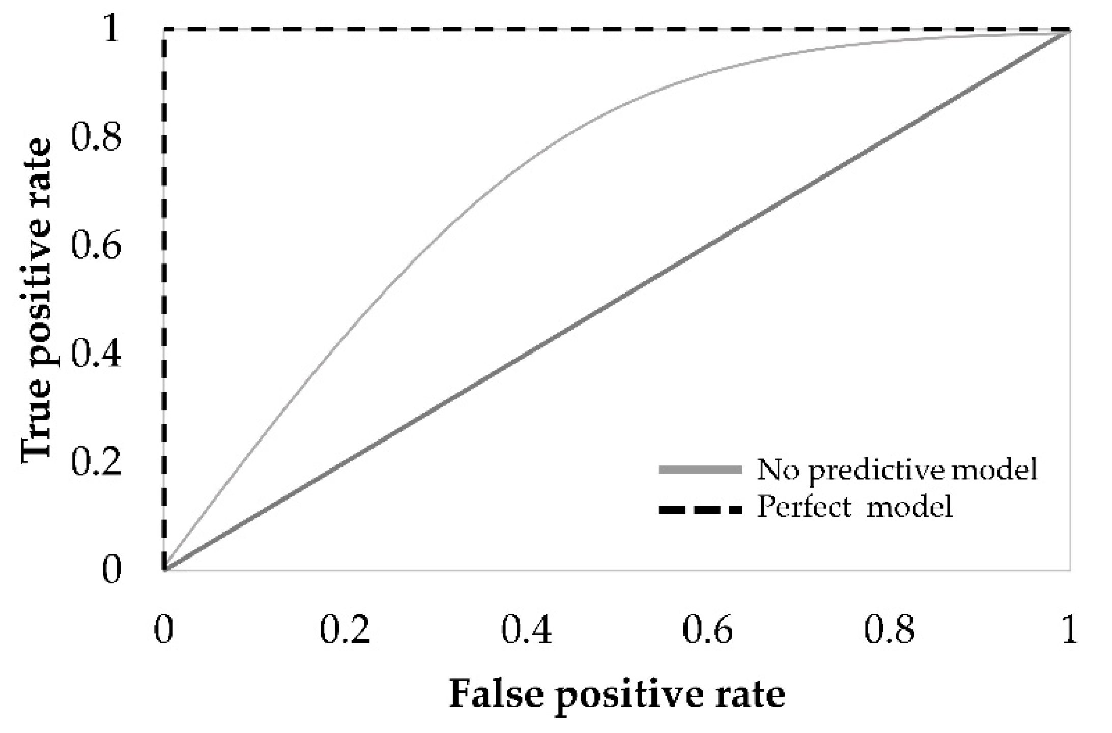
The ROC curve is a helpful technique for visualizing and selecting the most suitable model based on performance [47]. This curve is obtained by plotting the TPR as a function of the FPR (Figure 1), considering different probability thresholds to make class predictions [39]. The ROC curve is considered reliable when the curve is over the 45° line. Perfect classification is graphically defined by the union of two lines, corresponding to FPR equal to 1 and TPR equal to 1 [9].

Generally, a baseline probability threshold, where any pipe with a predicted probability of failure greater than 50% will be assigned as failed, is used to train the models. A new threshold can be determined using Youden’s J index.

$$\mathrm{J}=\mathrm{Sensitivity}+\mathrm{Specificity}-1=\mathrm{TPR}+\mathrm{TNR}-1$$

(22)

This index allows a new threshold that is closest to the optimal model. Youden’s J index does not modify the trained model as the same parameters are being used, and it is only employed to increase the sensitivity of the model to the minority class of interest [48].

2.2. Case Study

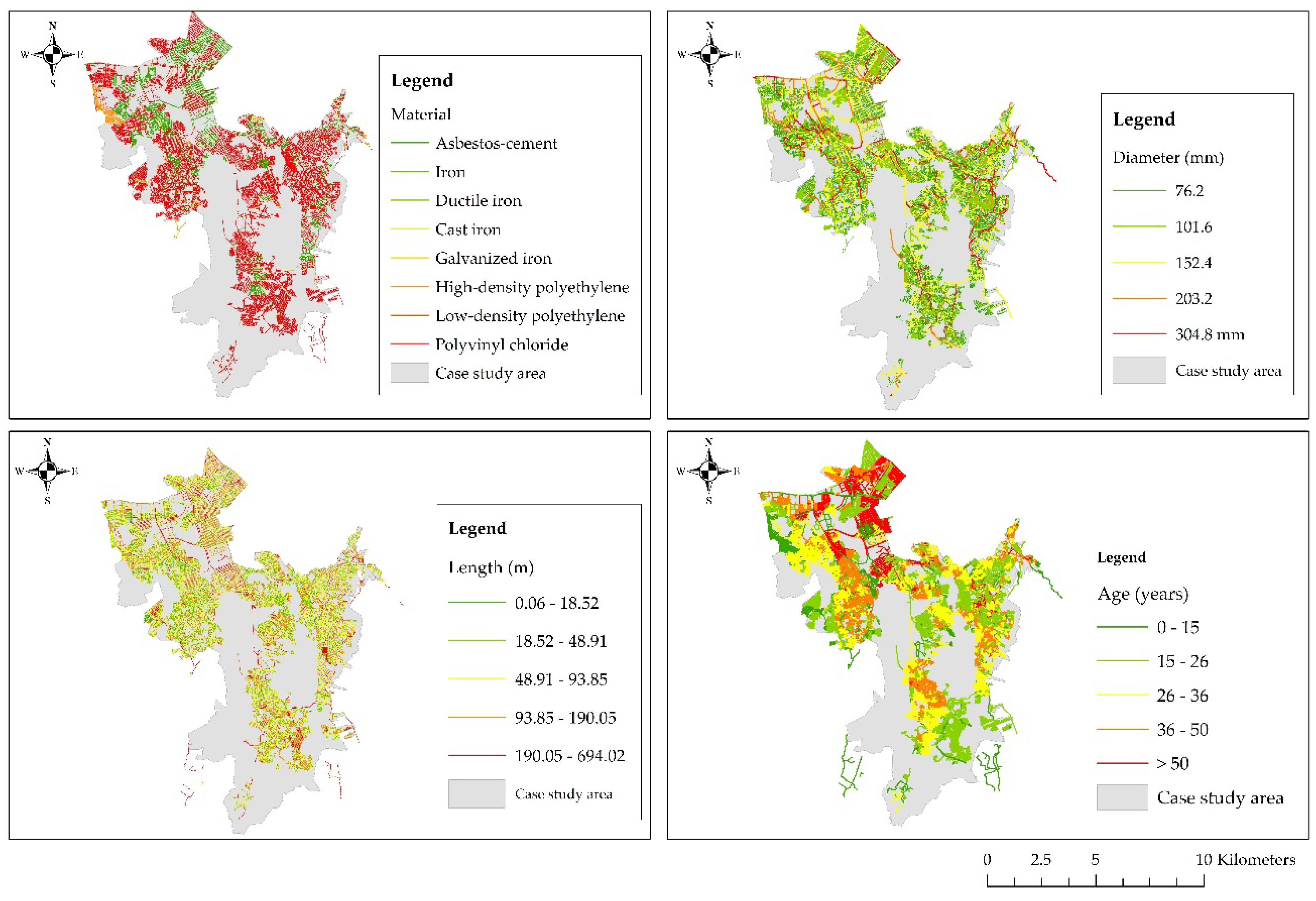
The proposed models were applied to a WDN in Bogotá (Colombia), presented in Figure 2. The WDN has 61,251 pipes with an overall network length of 1819 km and 28,671 house connections. The network has different pipe materials, distributed as follows: polyvinyl chloride (70.6%), asbestos-cement (24.2%), high-density polyethylene (2.7%), cast iron (0.9%), and others (1.6%). The average pipe is 29 years old, including the 11,442 pipes that have been in operation for over 40 years. The oldest pipes on the network are asbestos-cement (see Figure 2), and the majority of the pipes installed within the past 10 years are made of polyvinyl chloride (PVC). Pipe diameters range from 50.8 to 609.6 mm and approximately 51% of the pipes have a diameter ranging between 50.8 and 76.2 mm.

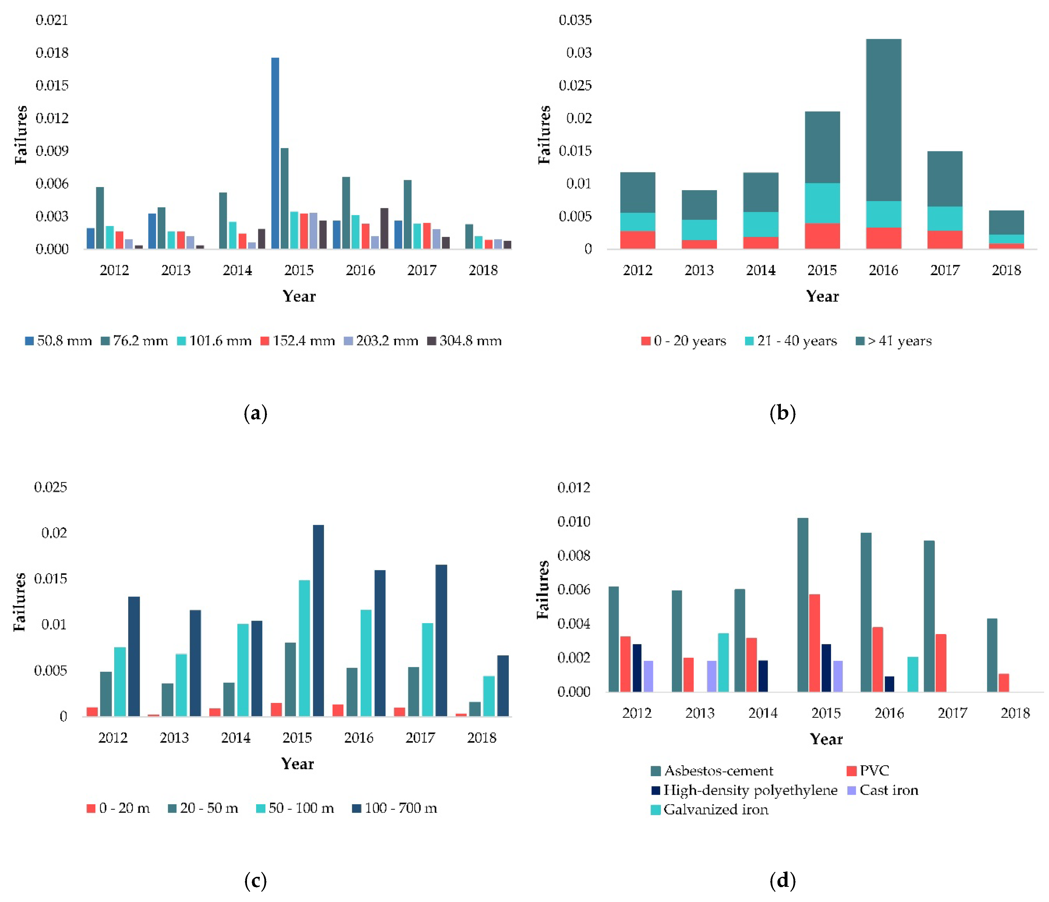
Pipe failure records, available from 2012 to 2018, were provided by the city’s water utility service (EAB). Figure 3 shows the relationship between failures and the pipes’ characteristics. A preliminary analysis showed that pipes with diameters of between 50.8 and 76.2 mm exhibited the highest failure rate (see Figure 3a). Commonly, the number of failures in small diameter pipes exceeds that of larger diameter pipes [5,49]. The main reason for the higher frequency of failure in small diameter pipes has been attributed to decreased pipe strength to ground movement and corrosion because of reduced wall thickness [50]. As presented in Figure 3b, the older pipes showed a higher number of failures. Failure rates can be expected to be higher in the months following the installation. Then, the rates are lower for several years, before increasing with the age of the pipe [50]. Pipe deterioration with age is known to occur. Nevertheless, the relationship between the pipe age and the failure rate is not clear due to manufacturing process, installation and operational practices, and environmental conditions. In the network, the average age of pipe failure is 34 years. The analysis also exhibited that the failure rate increased with the pipe length (see Figure 3c). Boulos et al. [51] concluded that short pipes broke less than longer pipes because a short pipe length limits the effects of transient surge pressure because junctions cause pressure wave reflections.

In addition, Figure 3d shows the number of failures per material normalized by the total number of pipes of each material. Failure records revealed that 67.8% of the failed pipes are made of asbestos-cement and 28.3% of PVC. The failure rate of pipe materials is determined by the material’s flexibility, method of manufacture, and manufacturing processes [50]. It was expected that PVC pipes have a lower failure rate than asbestos-cement pipes because plastic materials were the last to be introduced, and their quality has improved significantly over the years. The higher number of failures exhibited by asbestos-cement and PVC pipes also depends on the material distribution, which is described above. Based on these findings, only asbestos-cement and PVC pipes are considered for the analysis. As each type of material has a specific deterioration pattern [9,52], independent (per material) analyses were carried out for each.

3. Results and Discussion

3.1. Statistical Models

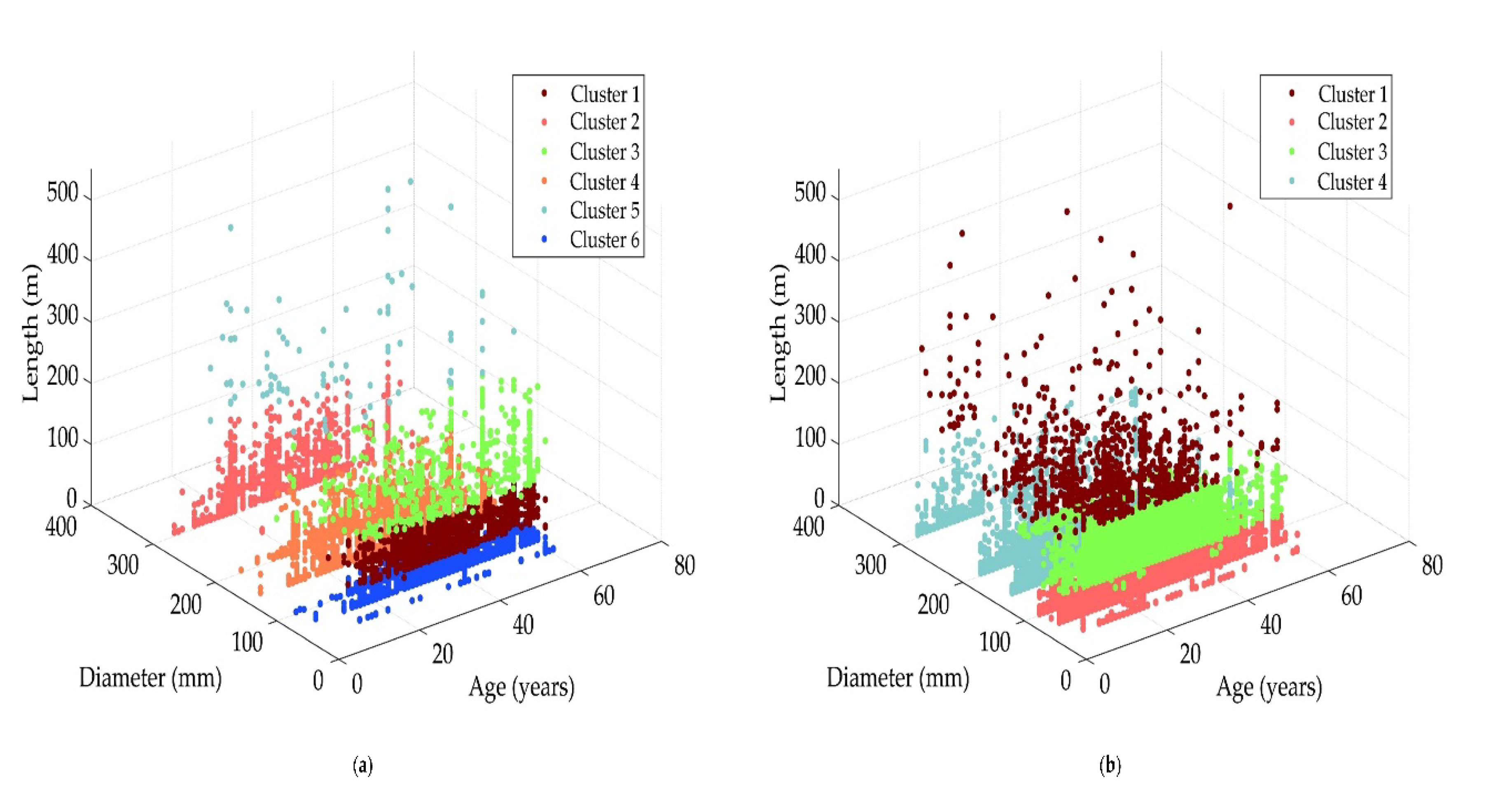
Regarding the statistical models, the K-means clustering approach was applied to separate the data into a number of specified clusters based on pipe diameter, length, and age. Other variables were excluded as using the pipes’ attributes helps to obtain models with greater statistical significance [5,53]. To determinate the optimal number of clusters, the Davies–Bouldin criterion was applied. Thus, the data were divided into six groups for asbestos-cement pipes and four groups for PVC pipes. The DBI calculated for the clustering was 0.6478 and 0.6322 for asbestos-cement and PVC pipes, respectively. The K-means algorithm was run using different initializations of centroids, and the partition that produced the lower sum of squared distance was chosen. Optimal partitions results and the distribution of the data set for the number of clusters calculated are shown in Figure 4. The diameter was the variable that most influenced the partition, followed by the length. The data points of each cluster have a high similarity to each other in terms of diameter and length. As shown in Figure 4, the clusters are composed of pipes with different ages, which could mean that age is not being a good indicator of the pipe condition.

Table 3. Results for Linear and Poisson regression.

Variable	Asbestos-Cement				PVC
	Linear Regression		Poisson Regression		Linear Regression		Poisson Regression
	$\mathit{\beta }$	p-Value	$\mathit{\beta }$	p-Value	$\mathit{\beta }$	p-Value	$\mathit{\beta }$	p-Value
Diameter (mm)	−0.457	0.000	−0.074	0.000	−0.401	0.000	−0.009	0.000
Length (km)	2.707	0.000	0.034	0.000	0.919	0.000	0.002	0.000
Age (years)	0.162	0.000	−0.001	0.008	0.679	0.000	−0.001	0.000
Intercept	n/a	n/a	4.466	0.001	n/a	n/a	5.810	0.000

and

Table 4. Results for Evolutionary Polynomial Regressions (EPR).

Material	Equation
Asbestos-cement	$\mathrm{FR}={0.202L}^{1.5}{/\mathrm{DA}}^2$
PVC	$\mathrm{FR}={0.00795\mathrm{LA}}^{0.5}{/\mathrm{D}}^{0.5}$

L = Length (m), A = Age (years) and D = Diameter (mm).

summarize the obtained results for the statistical models. By comparison, the regression coefficients associated with the explanatory variables are relatively different among materials. The latter is because the pipe deterioration process is different among materials. Factors such as construction methods, corrosion processes, and environmental conditions can affect the relationship between pipe age, diameter, length, and number of failures for each material. Other authors have also observed differences in the fitted values of the variables from one to another material [49,54]. From the reported values, pipe length proved to be highly relevant in the observed failure events. The applied methods showed an inverse relationship between the diameter and the number of failures. Furthermore, pipe length has a positive relationship with the number of failures. These relationships are consistent with previous research [5,49,53]. In contrast, three of the equations exhibited a positive relationship between pipe age and the failures, while the remaining presented an inverse relationship. This is a counterintuitive result, considering that older pipes are most likely to fail. However, this can be explained by the fact that many pipes are older than the point in time when pipe failures began to be recorded [14]. Other authors have attributed this result to the fact that only measurable variables are included in the models. Variables such as quality and strength of the material are not measured, but their change can produce variations in pipe performance from one age to another [14,55].

Table 5. Comparison of model performance.

Performance Metric	Dataset	Linear Regression	Poisson Regression	EPR
R2	Train data	0.693	0.923	0.877
	Test data	0.695	0.927	0.885
RMSE	Train data	45.31	22.87	31.12
	Test data	44.93	22.09	31.10

presents a summary of the statistical models’ performance. All the models showed acceptable performance on both training and testing datasets. Poisson Regression performs best according to R² and RMSE. These results confirmed that the Poisson Regression’s ability for generalization (i.e., the model’s ability to adapt properly to a new range of inputs) is better than that of the other techniques. The advantage of the Poisson Regression is to recognize the non-negative nature of the predicted variable. The application of this model is suitable for predicting failures in pipes with lower failure rates, such as pipes with large diameters and small lengths.

Because the number of failures should be assessed for each pipe over a certain period, the models trained cannot be used directly for calculating the failure rate for an individual pipe because they are aggregated. The individual failure rate (λ_i) for a given observation period (T) is calculated by considering the pipe length (L_i), the total class length (L_group), and the failures predicted for the group (FR_group) [5].

$${\mathsf{\lambda }}_{\mathrm{i}}=\frac{{\mathrm{FR}}_{\mathrm{group}}}{\mathrm{T}}*\frac{{\mathrm{L}}_{\mathrm{i}}}{{\mathrm{L}}_{\mathrm{group}}}$$

(23)

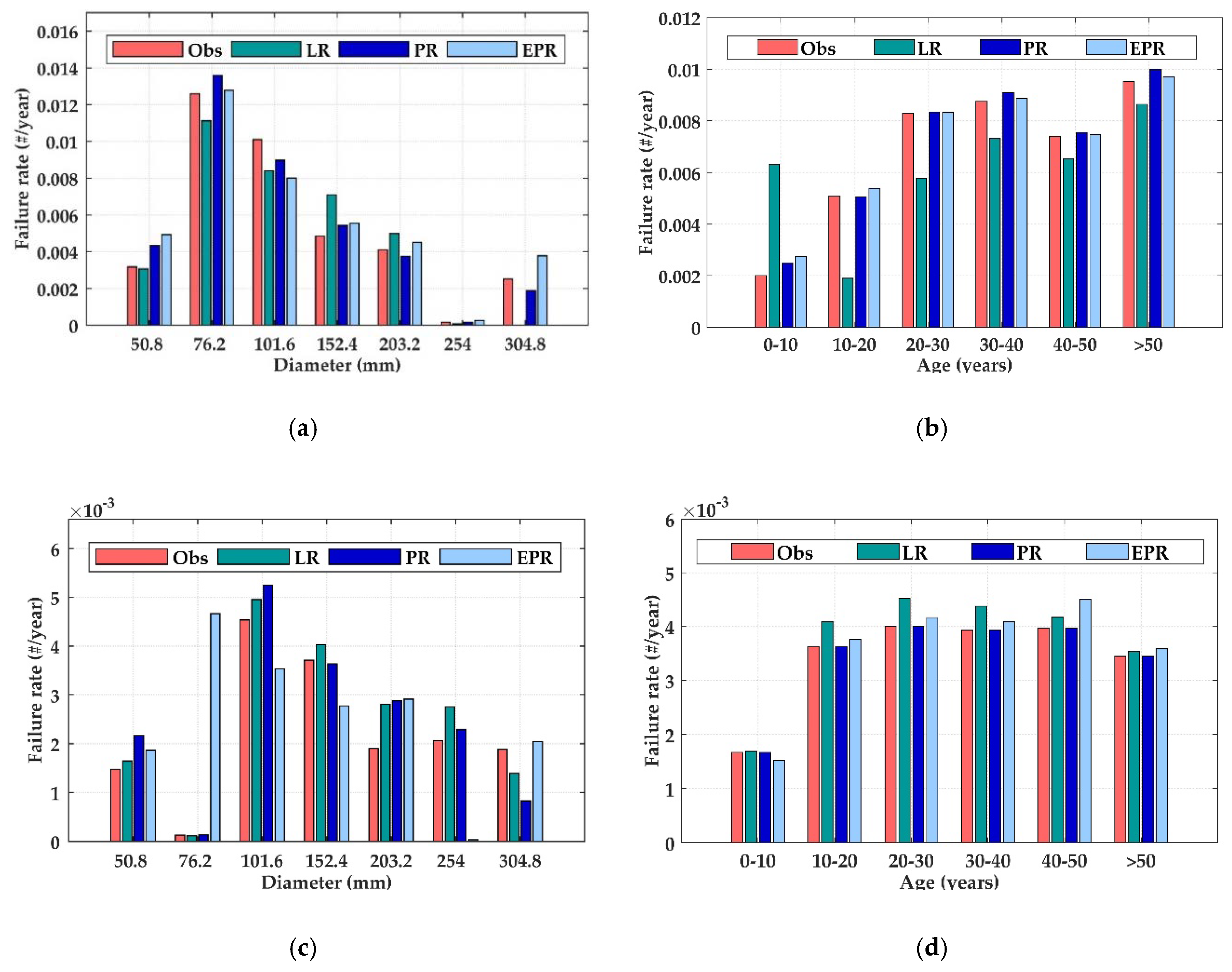
It is important to clarify that the failure rate does not consider the burst history of the individual pipe but the group of pipes. The accuracy of the individual failure rate predictions based on different pipe characteristics is compared in Figure 5. For the asbestos-cement pipes, Linear Regression underestimated the failure rate in most cases. The limitation of this model is more evident in younger pipes and pipes with larger diameters (see Figure 5a,b). Additionally, Poisson Regression and EPR showed adequate precision when calculating the failure rate in different age ranges and pipe diameters. Regarding the PVC pipes, the predicted capability of EPR is limited for the small pipe diameters (i.e., 76.2 mm), as shown in Figure 5c. This prediction has substantially improved for Poisson and Linear Regression. All the models show reasonable accuracy when calculating the failure rate in the different age ranges (see Figure 5d). Based on the results, the Poisson Regression is better than the two other models, while the quality of the Linear Regression and EPR are similar.

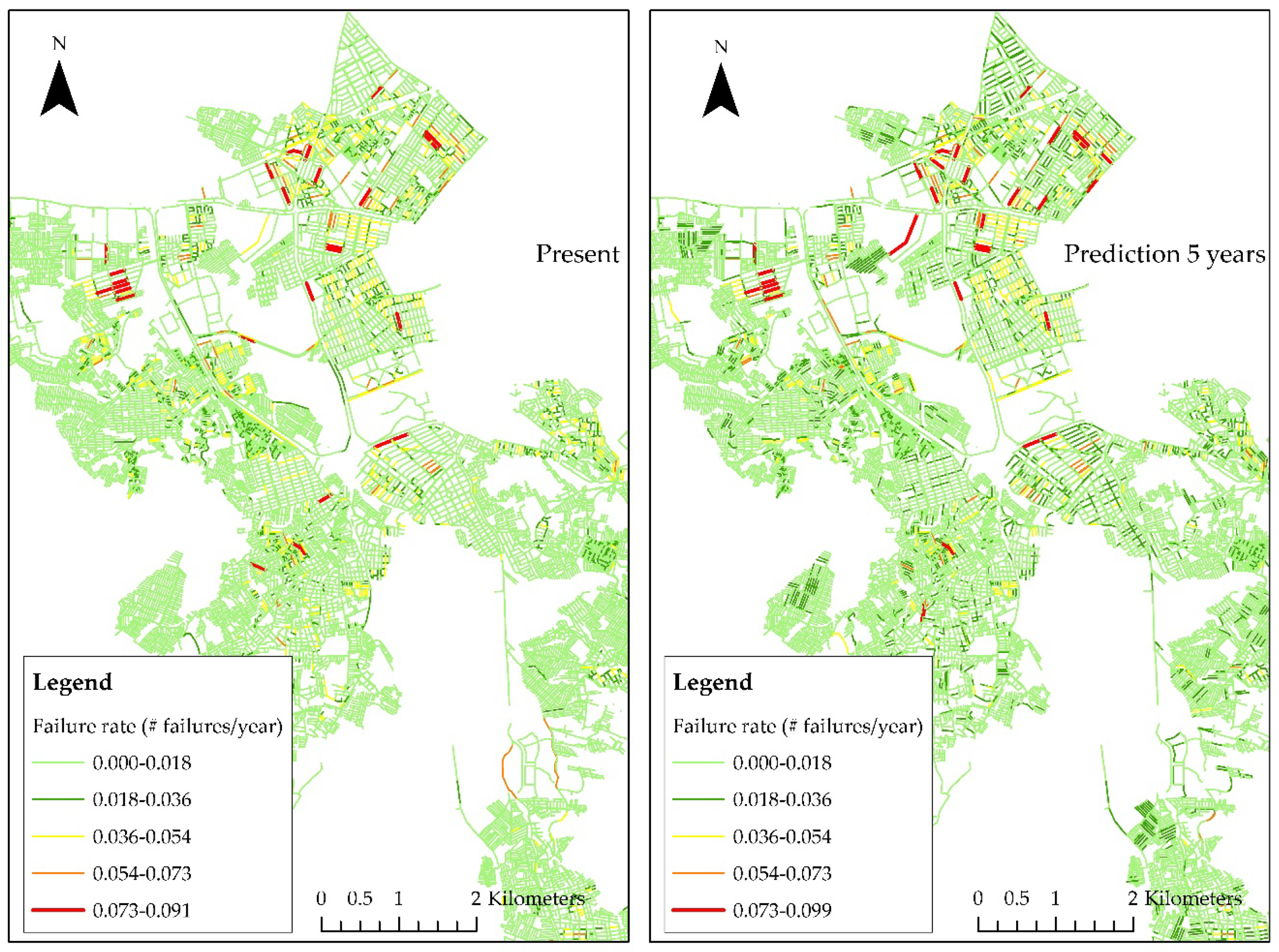
Based on the results, the best performance models were used to represent pipe failure rates in the WDN and classify them in different ranges to identify more vulnerable regions. Figure 6 shows the spatial distribution of the failure rates. The results showed that 4% and 5% of the pipes have a high failure rate in the current and predicted condition, respectively. The water utility service must pay attention to those pipes and take an appropriate preventive approach (e.g., maintenance or replacement after inspection). Further, for both current and predicted conditions, most of the pipes exhibit low failure rates. The approach presented above is useful for pipe failure prediction when information about other variables different from pipe attributes (e.g., environmental and operational variables such as water pressure and temperature) is not available. It is recommended to determine an appropriate group size according to the data characteristics to ensure that the aggregation process has statistical significance.

3.2. Machine Learning Models

With respect to ML models,

Table 6. Accuracy and the F-measure.

Model	Accuracy		F-measure
	Asbestos-Cement	PVC	Asbestos-Cement	PVC
Bayes	94.83%	93.69%	25.66%	6.26%
GBT	99.52%	99.79%	72.00%	46.43%
SVM	99.47%	99.83%	66.67%	52.18%
ANN	98.99%	99.61%	42.10%	7.40%

summarizes the accuracy and the F-measure for the trained models evaluated on the test data.

Table 7. Confusion matrices for the asbestos-cement pipes test sample.

Bayes		Predicted			GBT		Predicted
		Yes	No	Recall(%)			Yes	No	Recall(%)
Actual	Yes	39	6		Actual	Yes	27	14
	No	220	4106	86.67		No	7	4323	65.85
	Precision (%)	15.06	99.85	94.91		Precision (%)	79.41	99.68	99.84
SVM		Predicted			ANN		Predicted
		Yes	No	Recall(%)			Yes	No	Recall(%)
Actual	Yes	23	18	56.10	Actual	Yes	16	25	39.02
	No	5	4325	99.88		No	19	4311	99.56
	Precision (%)	82.14	99.59			Precision (%)	45.71	99.42

and

Table 8. Confusion matrices for the PVC pipes test sample.

Bayes		Predicted			GBT		Predicted
		Yes	No	Recall(%)			Yes	No	Recall(%)
Actual	Yes	27	1	96.69	Actual	Yes	13	15	46.43
	No	807	11977	96.43		No	15	12769	99.88
	Precision (%)	3.24	99.99			Precision (%)	46.43	99.88
SVM		Predicted			ANN		Predicted
		Yes	No	Recall(%)			Yes	No	Recall(%)
Actual	Yes	2	26	7.14	Actual	Yes	12	16	42.86
	No	24	12760	99.81		No	6	12778	99.95
	Precision (%)	7.69	99.80			Precision (%)	66.67	99.87

summarize the confusion matrices for the trained models. All the models used a baseline probability threshold where any pipe with a predicted failure probability of greater than 50% would be assigned as failed. Although the accuracy was higher than 93%, the confusion matrices revealed that ANNs focused on correctly classifying the majority class, namely the pipes that do not fail. Thus, ANNs gave only 39% of correct classifications for asbestos-cement failing pipes and 7.14% for PVC failing pipes. Overall accuracy may not afford a reliable performance indicator for models trained using an imbalanced dataset (i.e., when most of the pipes do not fail) because it can provide an incorrect impression of the capabilities to predict the minority class condition, in this case, the failing pipes. In contrast, the F-measure has demonstrated its usefulness to test the models’ performance when an imbalanced dataset is used for training. According to this metric, GBT and SVM showed acceptable performance.

In contrast, Bayes and GBT exhibited the best performance considering the TPR (e.g., 0.894 and 0.546 for asbestos-cement, respectively). The models with the lowest FPR were SVMs (0.179 for asbestos-cement and 0.333 for PVC) and GBT (0.265 for asbestos-cement and 0.535 for PVC). For failure prediction, conservative models are preferred because they reduce the pipes replacement cost before the end of their service life [9]. Although SVMs and GBT have a lower TPR compared to Bayes, using these models does not affect the rehabilitation strategies because not all pipes predicted to fail would be replaced immediately.

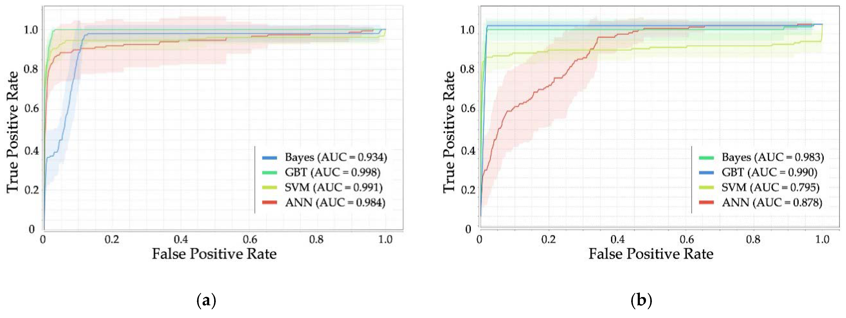
Figure 7 shows the ROC curves for the trained models. The caption provides information about the area under the curve (AUC), which is a quantity that falls in the range between zero and one that integrates over the respective ROC function [9]. Thus, if a comparison is made between models, the most effective model is the one with the largest AUC. For asbestos-cement pipes, the ROC curves for the four selected models are relatively close. GBT achieves the highest AUC (0.998), which indicates that this method is well suited for pipe failure prediction, and ANNs exhibit the lowest AUC (0.984). Concerning PVC pipes, ROC curves for GBT and Bayes are notably close, with the most reliable prediction model being GBT (see Figure 7). The results showed that these models discriminate better between failing pipes and nonfailing ones because its curve is always above the 45° line. Additionally, GBT exhibited the highest AUC and ANNs, the lowest.

As previously mentioned, all the trained models use a baseline probability of 50%. A new threshold can be determined using Youden’s J index. The value of the index for the GBT method was 0.57 and 0.54 for asbestos-cement and PVC pipes, respectively. The result suggested that, when applying GBT, acceptable predictions can be obtained for the failing pipes without sacrificing a reasonable level of accuracy for the pipes that do not fail.

By comparison, GBT exhibited better performance than the other models. This approach has the advantage of providing greater importance to the misclassified pipes in each iteration, so it not only focuses on correctly classifying the pipes that do not fail. As compared to SVM, GBT provides a higher level of readability and transparency of the result, and identifies the relevance of the explanatory variables. Additionally, Bayes was demonstrated to be an effective model for classifying the failing pipes. Despite this, the model showed the highest FNR (0.848 and 0.967 for asbestos-cement and PVC pipe datasets, respectively) and the lowest F-measure (25.66% and 6.26% for asbestos-cement and PVC pipe datasets, respectively). As mentioned earlier, the application of models with low FNR is preferable.

Results also showed that the imbalance dataset significantly compromised the ability of ANNs to correctly classify the failing pipes. The low predictive capability is most evident in PVC pipes (F-measure of 7.40%), as these pipes are less likely to fail, and they have been installed more recently. St. Clair et al. [56] and Wu et al. [6] mention that the data requirement is the main limitation of the ANNs.

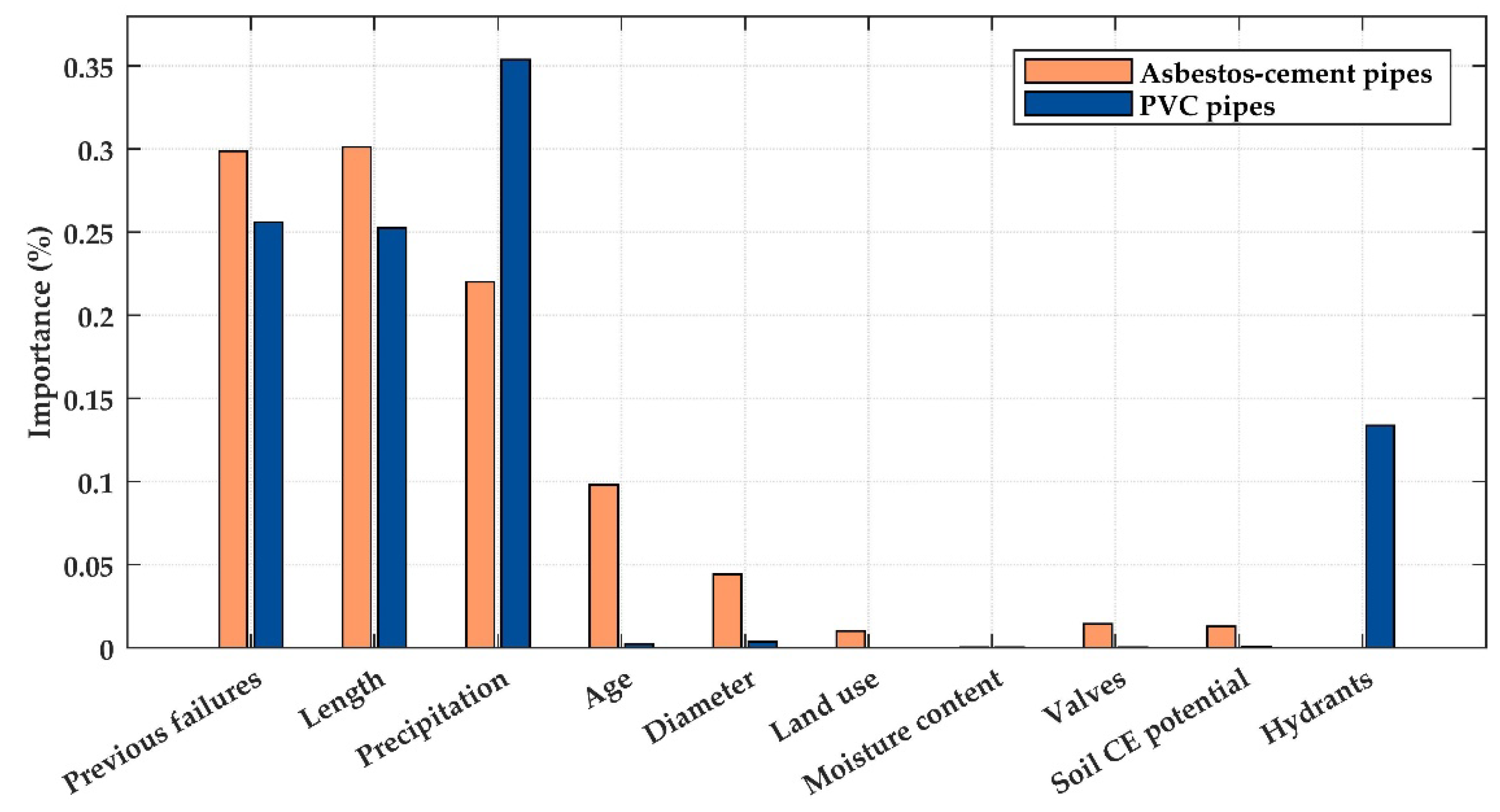
Figure 8 shows the importance of the variables for the GBT model, where high values indicate high relevance for the prediction process. The most important variables were the number of previous failures, length, and precipitation. Some authors found that the number of previous failures was a significant variable for predicting future failure rates and demonstrated their impact on the occurrence of new pipe failures [37,47,57]. Oliveira et al. [58] concluded that inadequate repairs of breaks might produce new failures close to the previous ones. Besides, Debón et al. [47] and Winkler et al. [9] also observed that pipe attributes, such as age, length, and diameter, are significant variables for failure prediction. The other environmental and operational selected variables were not particularly significant in the modeling process (see Figure 8). It is necessary to consider that because of the procedure’s data dependency, the importance of the variables is representative of this case study and not for the pipe failure process.

Because the other selected approaches cannot identify the significant variables in the modeling process, the backward elimination technique was used to recognize the relevance of the variables. This technique begins with a full model that contains all the selected variables for the modeling process. Variables are then removed one by one from the full model until all remaining variables are considered to have some significant contribution to the outcome [59]. The soil moisture content, soil contraction and expansion potential, and number of valves and hydrants connected to the pipe were the variables not considered for the asbestos-cement trained models. For the PVC pipes, the soil moisture content and soil contraction and expansion potential were eliminated from the SVM model. Further, the land use, soil moisture content, and soil contraction and expansion potential were excluded from the ANN model. In general, the results showed that environmental variables, such as the soil moisture content, land use, and soil contraction and expansion potential, have no pleasing effect on pipe failure modeling.

The GBT models trained were selected as the final classifiers due to their performance. A sensitivity analysis of GBT to the input variables was performed to provide information on its generalizability. The analysis was carried out considering the effects of variation in values of only one input, while the others remained constant. The results showed that the GBT model trained for asbestos-cement pipes is more sensitive to changes in the diameter, age, and the number of previous failures. An increase in the diameter, precipitation, and number of valves generates an increment in the number of failing pipes. The GBT model trained for PVC pipes is more sensitive to the number of previous failures, precipitation, and the number of hydrants. Modification of the other variables does not affect the outcome of pipes predicted to fail.

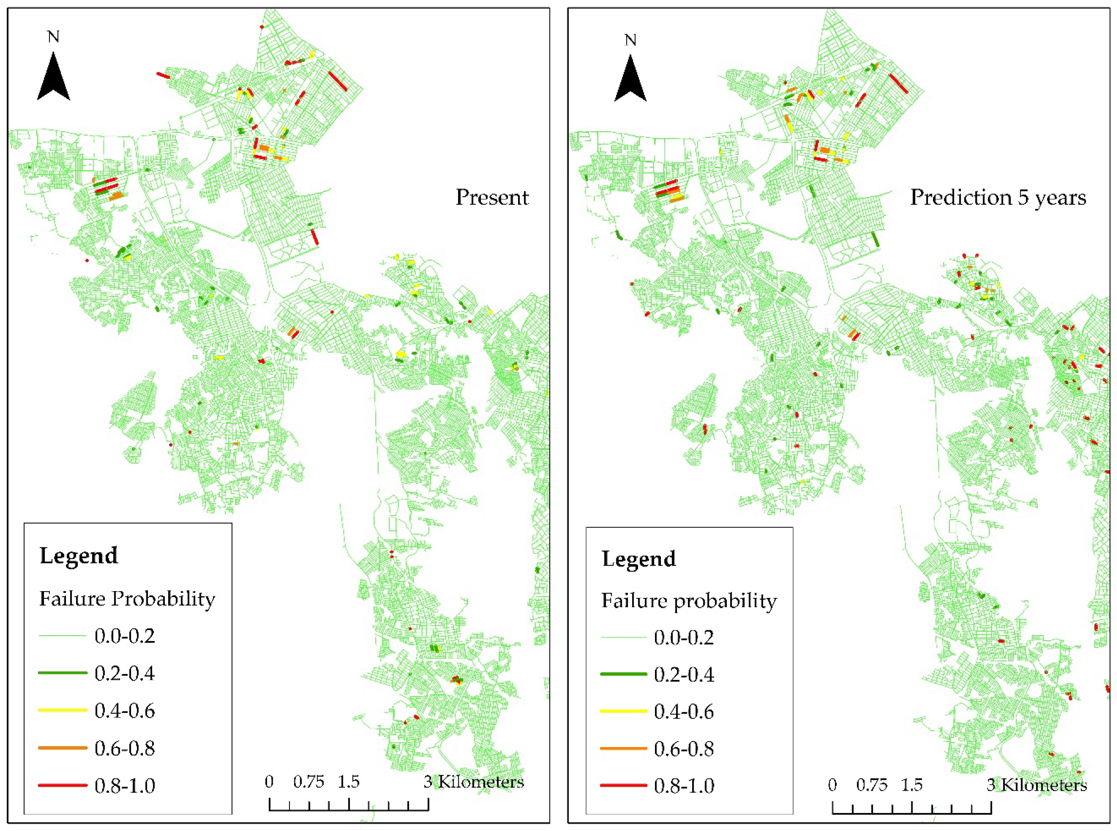
Based on the results, the final GBT models trained are used to predict the failure probability of individual pipes in the WDN. This prediction focuses on a specific pipe and its characteristics, which enables an understanding of a single pipe failure pattern. Figure 9 shows the pipes’ deterioration pattern in the WDN. The results revealed that around 0.17% of the pipes have a high probability of failure in the present condition. For those pipes, it is necessary to use the appropriate maintenance or replacement strategies to avoid failure. Likewise, for both current and predicted conditions, most of the pipes exhibit low failure probability. The analysis of the probability values made it possible to establish that, when comparing the current condition with the predicted condition, there was a 28% increase in the number of pipes with failure probabilities of between 0.6 and 0.8, and an 18% increase in the pipes with failure probabilities of between 0.8 and 1.0.

According to Figure 9, it is important to highlight that some pipes do not deteriorate as expected, as their condition improves with age. This can be explained by the fact that, when the age of the pipe is increased, observations outside of the training data are generated. Thus, the model requires an extrapolation of the predictions [9]. Although it is not intuitive, a decrease of the failure probability can be observed in reality. Some authors associate a higher failure rate with a pipe’s initial service life. [9,60]. Martinez-Codina et al. [61] performed a study to determine the relationship between pipe failure causes and processes. Based on the experimental analyses, they observed that the failure probability amounted to a higher rate in the first years of service life than in the later years.

The best performance models (i.e., Poisson regression for group pipe analysis and the GBT approach for individual pipe analysis) were applied to another WDN in Bogotá (Colombia). The WDN has 20,793 pipes with an overall network length of 652 km. The network has different pipe materials, distributed as follows: polyvinyl chloride (74.5%), asbestos-cement (25%), and concrete cylinder pipes (0.19%). Pipe diameters range from 50.8 to 406.4 mm, and 40% of the pipes have a diameter of 76.2 mm. In addition, approximately 75% of the pipes have an age ranging between 41 and 50 years. Pipe failure records are available from 2015 and 2017. A preliminary analysis showed that pipes with a diameter of 76.2 mm and an age of over 40 years exhibited the highest failure rate. Failure records revealed that 65% of the failed pipes are made of asbestos-cement and 34% of PVC.

Regarding the group pipe analysis, data were divided into four groups for both asbestos-cement and PVC pipes. Results show an R² of 0.452 for asbestos-cement pipes and 0.724 for PVC pipes. For the individual pipe analysis, results gave only 4% correct classifications for asbestos-cement pipe failure and 15% for PVC pipe failure. These results and other findings in previous studies underline the need for each WDN to develop its own failure model [1,62]. All the networks have substantive differences, and the effect of specific variables in the models is dependent on the WDN characteristics.

4. Conclusions

In this paper, the performance of several statistical and ML models in predicting pipe failure in WDNs was evaluated. Three statistical models, including Linear Regression, Poisson Regression, and Evolutionary Polynomial Regressions, were used for failure prediction based on pipe diameter, pipe age, and length as explanatory variables. ML approaches, including Gradient-Boosted Tree (GBT), Bayes, Support Vector Machine, and Artificial Neuronal Networks (ANNs), were compared in terms of their capability to predict individual pipe condition. Pipe attributes, and environmental and operational variables were included as input variables. The selected case study was a highly populated area in Bogotá with a large WDN.

The results of the statistical models showed that the cluster-based prediction approach reduces the prediction error for pipe failure when information about variables other than pipe attributes is not available. All the models demonstrated acceptable results in terms of their performance (R² between 0.695 and 0.927 and RMSE between 45 and 22 for the test sample), but the application of Poisson Regression was the most suitable for predicting failures in pipes with lower failure rates. Regarding ML models, all methods but the ANNs presented acceptable performance. The GBT approach presented the best performing classifier (ACU of 0.998 and 0.990 for the test sample of asbestos-cement and PVC pipes, respectively). The GBT model has a greater ability to accurately predict pipe failure when an imbalanced database is used. Furthermore, the assumptions and trade-offs of the GBT model are more transparent than in other artificial intelligence techniques.

Using the abovementioned predictive models earlier could significantly reduce the time and money allocated to the identification of deteriorated pipes. The group-pipe failure analysis is useful when the available data is limited. In contrast, the individual-pipe approach makes it possible to consider the single pipe failure history, which is of great importance for establishing an individual pipe’s propensity to fail. The knowledge provided by this study is especially important for water utility as it provides information that helps to prioritize a proactive rehabilitation strategy, making it more efficient and profitable. Future work will include the application of the modeling approach to a more detailed dataset that incorporates other variables such as water pressure and temperature, which affect the pipe failure process [63,64]. It is also recommended to evaluate the effect of the failures’ spatial correlation [65].

References

- Tabesh, M.; Soltani, J.; Farmani, R.; Savic, D. Assessing pipe failure rate and mechanical reliability of water distribution networks using data-driven modeling. J. Hydroinform. 2009, 11, 1–17. [Google Scholar] [CrossRef]
- Martins, A.; Leitão, J.P.; Amado, C. Comparative study of three stochastic models for prediction of pipe failures in water supply systems. J. Infrastruct. Syst. 2013, 19, 442–450. [Google Scholar] [CrossRef]
- Giudicianni, C.; Herrera, M.; di Nardo, A.; Carravetta, A.; Ramos, H.M.; Adeyeye, K. Zero-net energy management for the monitoring and control of dynamically-partitioned smart water systems. J. Clean. Prod. 2020, 252, 119745. [Google Scholar] [CrossRef]
- Ilaya-Ayza, A.E.; Martins, C.; Campbell, E.; Izquierdo, J. Implementation of DMAs in intermittent water supply networks based on equity criteria. Water 2017, 9, 851. [Google Scholar] [CrossRef] [Green Version]
- Berardi, L.; Giustolisi, O.; Kapelan, Z.; Savic, D.A. Development of pipe deterioration models for water distribution systems using EPR. J. Hydroinform. 2008, 10, 113–126. [Google Scholar] [CrossRef] [Green Version]
- Wu, Y.; Liu, S. A review of data-driven approaches for burst detection in water distribution systems. Urban Water J. 2017, 14, 972–983. [Google Scholar] [CrossRef]
- Nogueira Vilanova, M.R.; Filho, P.M.; Perrella Balestieri, J.A. Performance measurement and indicators for water supply management: Review and international cases. Renew. Sustain. Energy Rev. 2014, 43, 1–12. [Google Scholar] [CrossRef]
- El Tiempo El 36% del Agua Que se Consume en Bogotá No se Factura. Available online: https://www.eltiempo.com/bogota/empresa-de-acueducto-y-alcantarillado-de-bogota-habla-de-la-las-facturas-que-no-se-pagan-99578 (accessed on 22 June 2018).
- Winkler, D.; Haltmeier, M.; Kleidorfer, M.; Rauch, W.; Tscheikner-Gratl, F. Pipe failure modelling for water distribution networks using boosted decision trees. Struct. Infrastruct. Eng. 2018, 14, 1402–1411. [Google Scholar] [CrossRef] [Green Version]
- Rajani, B.; Kleiner, Y. Comprehensive review of structural deterioration of water mains: Physically based models. Urban Water 2001, 3, 151–164. [Google Scholar] [CrossRef] [Green Version]
- Scheidegger, A.; Leitão, J.P.; Scholten, L. Statistical failure models for water distribution pipes—A review from a unified perspective. Water Res. 2015, 83, 237–247. [Google Scholar] [CrossRef]
- Pelletier, G.; Milhot, A.; Villeneuve, J.P. Modeling water pipe breaks—Three case studies. J. Water Resour. Plan. Manag. 2003, 129, 115–123. [Google Scholar] [CrossRef]
- Rajani, B.; Kleiner, Y. Comprehensive review of structural deterioration of water mains: Statistical models. Urban Water 2001, 3, 131–150. [Google Scholar] [CrossRef] [Green Version]
- Kakoudakis, K.; Behzadian, K.; Farmani, R.; Butler, D. Pipeline failure prediction in water distribution networks using evolutionary polynomial regression combined with K-means clustering. Urban Water J. 2017, 14, 737–742. [Google Scholar] [CrossRef]
- Alvisi, S.; Franchini, M. Comparative analysis of two probabilistic pipe breakage models applied to a real water distribution system. Civ. Eng. Environ. Syst. 2010, 27, 1–22. [Google Scholar] [CrossRef]
- Wilson, D.; Filion, Y.; Moore, I. State-of-the-art review of water pipe failure prediction models and applicability to large-diameter mains. Urban Water J. 2017, 14, 173–184. [Google Scholar] [CrossRef]
- Motiee, H.; Ghasemnejad, S. Prediction of pipe failure rate in Tehran water distribution networks by applying regression models. Water Sci. Technol. Water Supply 2019, 19, 695–702. [Google Scholar] [CrossRef] [Green Version]
- Jafar, R.; Shahrour, I.; Juran, I. Application of Artificial Neural Networks (ANN) to model the failure of urban water mains. Math. Comput. Model. 2010, 51, 1170–1180. [Google Scholar] [CrossRef]
- Zangenehmadar, Z.; Moselhi, O. Assessment of Remaining Useful Life of Pipelines Using Different Artificial Neural Networks Models. J. Perform. Constr. Facil. 2016, 30, 04016032. [Google Scholar] [CrossRef]
- Aydogdu, M.; Firat, M. Estimation of Failure Rate in Water Distribution Network Using Fuzzy Clustering and LS-SVM Methods. Water Resour. Manag. 2015, 29, 1575–1590. [Google Scholar] [CrossRef]
- Shirzad, A.; Safari, M.J.S. Pipe failure rate prediction in water distribution networks using multivariate adaptive regression splines and random forest techniques. Urban Water J. 2019, 16, 653–661. [Google Scholar] [CrossRef]
- Robles-Velasco, A.; Cortés, P.; Muñuzuri, J.; Onieva, L. Prediction of pipe failures in water supply networks using logistic regression and support vector classification. Reliab. Eng. Syst. Saf. 2020, 196, 106754. [Google Scholar] [CrossRef]
- Harvey, R.; McBean, E.A.; Gharabaghi, B. Predicting the timing of water main failure using artificial neural networks. J. Water Resour. Plan. Manag. 2014, 140, 425–434. [Google Scholar] [CrossRef]
- Ott, L. An Introduction to Statistical Methods and Data Analysis, 5th ed.; Duxbury and Wadsworth Publishing Co.: Belmont, CA, USA, 2001; Volume 34. [Google Scholar]
- Winkelmann, R. Econometric Analysis of Count Data, 5th ed.; Springer: Berlin, Germany, 2013; pp. 63–74. [Google Scholar]
- Kleiner, Y.; Nafi, A.; Rajani, B. Planning renewal of water mains while considering deterioration, economies of scale and adjacent infrastructure. Water Sci. Technol. Water Supply 2010, 10, 897–906. [Google Scholar] [CrossRef]
- Giustolisi, O.; Savic, D.A. A symbolic data-driven technique based on evolutionary polynomial regression. J. Hydroinform. 2006, 8, 207–222. [Google Scholar] [CrossRef] [Green Version]
- Fortunato, S. Community detection in graphs. Phys. Rep. 2010, 486, 75–174. [Google Scholar] [CrossRef] [Green Version]
- Kim, S.E.; Seo, I.W. Artificial Neural Network ensemble modeling with conjunctive data clustering for water quality prediction in rivers. J. Hydro-Environ. Res. 2015, 9, 325–339. [Google Scholar] [CrossRef]
- Xiao, J.; Lu, J.; Li, X. Davies Bouldin Index based hierarchical initialization K-means. Intell. Data Anal. 2017, 21, 1327–1338. [Google Scholar] [CrossRef]
- Wang, G.; Wang, Z.; Chen, W.; Zhuang, J. Classification of surface EMG signals using optimal wavelet packet method based on Davies-Bouldin criterion. Med. Biol. Eng. Comput. 2006, 44, 865–872. [Google Scholar] [CrossRef]
- Davies, D.; Bouldin, D. A Cluster Separation Measure. IEEE Trans. Pattern Anal. Mach. Intell. 1979, 2, 224–227. [Google Scholar] [CrossRef]
- Nicolas, P.R. Scala for Machine Learning: Leverage Scala and Machine Learning to Construct and Study Systems that Can Learn from Data, 1st ed.; Packt Publishing: Birmingham, UK, 2014; p. 57. [Google Scholar]
- Sousa, V.; Matos, J.P.; Matias, N. Evaluation of artificial intelligence tool performance and uncertainty for predicting sewer structural condition. Autom. Constr. 2014, 44, 84–91. [Google Scholar] [CrossRef]
- Friedman, J. Additive Logistic Regression: A Statistical View of Boosting. Ann. Stat. 2000, 28, 337–374. [Google Scholar] [CrossRef]
- Theodoridis, S. Classification: A tour of the classics. In Machine Learning; Theodoridis, S., Ed.; Academic Press: London, UK, 2015; pp. 275–325. [Google Scholar]
- Kabir, G.; Tesfamariam, S.; Francisque, A.; Sadiq, R. Evaluating risk of water mains failure using a Bayesian belief network model. Eur. J. Oper. Res. 2015, 240, 220–234. [Google Scholar] [CrossRef]
- Ogutu, G.A.; Okuthe, P.K.; Lall, M. A review of probabilistic modeling of pipeline leakage using Bayesian Networks. J. Eng. Appl. Sci. 2017, 12, 3163–3173. [Google Scholar]
- Harvey, R.R.; McBean, E.A. Comparing the utility of decision trees and support vector machines when planning inspections of linear sewer infrastructure. J. Hydroinform. 2014, 16, 1265–1279. [Google Scholar] [CrossRef] [Green Version]
- Kutyłowska, M.; Hotloś, H. Failure analysis of water supply system in the Polish city of Głogów. Eng. Fail. Anal. 2014, 41, 23–29. [Google Scholar] [CrossRef]
- Hastie, T.; Tibshirani, R.; Friedman, J. Linear Methods for Classification, 2nd ed.; Springer: New York, NY, USA, 2009; pp. 353–361. [Google Scholar]
- Belayneh, A.; Adamowski, J. Standard Precipitation Index Drought Forecasting Using Neural Networks, Wavelet Neural Networks, and Support Vector Regression. Appl. Comput. Intell. Soft Comput. 2012, 2012, 794061. [Google Scholar] [CrossRef]
- Naser, J.A. Neural networks—A brief introduction. Proc. Am. Power Conf. 1991, 53, 943–945. [Google Scholar]
- Theodoridis, S. Neural Networks and Deep Learning. In Machine Learning; Theodoridis, S., Ed.; Academic Press: London, UK, 2015; pp. 875–936. [Google Scholar]
- Laakso, T.; Kokkonen, T.; Mellin, I.; Vahala, R. Sewer condition prediction and analysis of explanatory factors. Water 2018, 10, 1239. [Google Scholar] [CrossRef] [Green Version]
- Luciani, C.; Casellato, F.; Alvisi, S.; Franchini, M. Green Smart Technology for Water (GST4Water): Water loss identification at user level by using smart metering systems. Water 2019, 11, 405. [Google Scholar] [CrossRef] [Green Version]
- Debón, A.; Carrión, A.; Cabrera, E.; Solano, H. Comparing risk of failure models in water supply networks using ROC curves. Reliab. Eng. Syst. Saf. 2010, 95, 43–48. [Google Scholar] [CrossRef]
- Harvey, R.R.; McBean, E.A. Predicting the structural condition of individual sanitary sewer pipes with random forests. Can. J. Civ. Eng. 2014, 41, 294–303. [Google Scholar] [CrossRef]
- Jenkins, L.; Gokhale, S.; McDonald, M. Comparison of pipeline failure prediction models for water distribution networks with uncertain and limited data. J. Pipeline Syst. Eng. Pract. 2015, 6, 04014012. [Google Scholar] [CrossRef]
- Barton, N.A.; Farewell, T.S.; Hallett, S.H.; Acland, T.F. Improving pipe failure predictions: Factors effecting pipe failure in drinking water networks. Water Res. 2019, 164, 114926. [Google Scholar] [CrossRef] [PubMed]
- Boulos, P.F.; Karney, B.W.; Wood, D.J.; Lingireddy, S. Hydraulic transient guidelines for protecting water distribution systems. J. Am. Water Work. Assoc. 2005, 97, 111–124. [Google Scholar] [CrossRef]
- Ahmadi, M.; Cherqui, F.; Aubin, J.B.; Le Gauffre, P. Sewer asset management: Impact of sample size and its characteristics on the calibration outcomes of a decision-making multivariate model. Urban Water J. 2016, 13, 41–56. [Google Scholar] [CrossRef]
- Xu, Q.; Chen, Q.; Li, W.; Ma, J. Pipe break prediction based on evolutionary data-driven methods with brief recorded data. Reliab. Eng. Syst. Saf. 2011, 96, 942–948. [Google Scholar] [CrossRef]
- Asnaashari, A.; McBean, E.A.; Shahrour, I.; Gharabaghi, B. Prediction of watermain failure frequencies using multiple and Poisson regression. Water Sci. Technol. Water Supply 2009, 9, 9–19. [Google Scholar] [CrossRef]
- Boxall, J.B.; O’Hagan, A.; Pooladsaz, S.; Saul, A.J.; Unwin, D.M. Estimation of burst rates in water distribution mains. Proc. Inst. Civ. Eng. Water Manag. 2007, 160, 73–82. [Google Scholar] [CrossRef]
- St. Clair, A.M.; Sinha, S. State-of-the-technology review on water pipe condition, deterioration and failure rate prediction models! Urban Water J. 2012, 9, 85–112. [Google Scholar] [CrossRef]
- Kleiner, Y.; Rajani, B. Comparison of four models to rank failure likelihood of individual pipes. J. Hydroinform. 2012, 14, 659–681. [Google Scholar] [CrossRef] [Green Version]
- De Oliveira, D.P.; Garrett, J.H.; Soibelman, L. A density-based spatial clustering approach for defining local indicators of drinking water distribution pipe breakage. Adv. Eng. Inform. 2011, 25, 380–389. [Google Scholar] [CrossRef]
- Ratner, B. Variable selection methods in regression: Ignorable problem, outing notable solution. J. Target. Meas. Anal. Mark. 2010, 18, 65–75. [Google Scholar] [CrossRef]
- Davies, J.P.; Clarke, B.A.; Whiter, J.T.; Cunningham, R.J. Factors influencing the structural deterioration and collapse of rigid sewer pipes. Urban Water 2001, 3, 73–89. [Google Scholar] [CrossRef]
- Martínez-Codina, Á.; Gómez, P.; de la Fuente, G. Relación entre las causas y los modos de fallo de tuberías en la red de distribución de Canal de Isabel II en Madrid. Rev. Iberoam. Agua 2018, 5, 16–28. [Google Scholar] [CrossRef] [Green Version]
- Demissie, G.; Tesfamariam, S.; Sadiq, R. Prediction of pipe failure by considering time-dependent factors: Dynamic Bayesian belief network model. J. Risk Uncertain. Eng. Syst. Part A Civ. Eng. 2017, 3, 04017017. [Google Scholar] [CrossRef]
- Rajani, B.; Kleiner, Y.; Sink, J.E. Exploration of the relationship between water main breaks and temperature covariates. Urban Water J. 2012, 9, 67–84. [Google Scholar] [CrossRef]
- Wols, B.A.; van Thienen, P. Impact of climate on pipe failure: Predictions of failures for drinking water distribution systems. Eur. J. Transp. Infrastruct. Res. 2016, 16, 240–253. [Google Scholar]
- Pulido, E.S.; Arboleda, C.V.; Rodríguez Sánchez, J.P. Study of the spatiotemporal correlation between sediment-related blockage events in the sewer system in Bogotá (Colombia). Water Sci. Technol. 2019, 79, 1727–1738. [Google Scholar] [CrossRef]
Figure 1.
The receiver operating characteristic (ROC) curve.
Figure 2.
Case study area in southern Bogotá (Colombia).
Figure 3.
Relationship between: (a) Pipe diameter and failures normalized by the number of pipes of each diameter; (b) Pipe age and failures normalized by the number of pipes of each age range; (c) Pipe length and failures normalized by the number of pipes of each length range; (d) Pipe material and failures normalized by the total of pipes of each material.
Figure 4.
Data clustering: (a) Asbestos-cement pipes and (b) polyvinyl chloride (PVC) pipes.
Figure 5.
Average observations and predictions of failure rate based on: (a) Asbestos-cement pipe diameter; (b) Asbestos-cement pipe age; (c) PVC pipe diameter; (d) PVC pipe age.
Figure 6.
Failure rate prediction in asbestos-cement and PVC pipes.
Figure 7.
ROC curve for failure pipes: (a) Asbestos-cement pipes; (b) PVC pipes.
Figure 8.
Comparison of explanatory variable relative importance.
Figure 9.
Predictions of the failure probability in asbestos-cement and PVC pipes.