Implementation of a Local Time Stepping Algorithm and Its Acceleration Effect on Two-Dimensional Hydrodynamic Models

Renewable Energy School, North China Electric Power University, Beijing 102206, China
*
Author to whom correspondence should be addressed.
Water 2020, 12(4), 1148; https://doi.org/10.3390/w12041148
Submission received: 11 February 2020
/
Revised: 26 March 2020
/
Accepted: 7 April 2020
/
Published: 17 April 2020
(This article belongs to the Special Issue Shallow Water Equations in Hydraulics: Modeling, Numerics and Applications)
Abstract
:The engineering applications of two-dimensional (2D) hydrodynamic models are restricted by the enormous number of meshes needed and the overheads of simulation time. The aim of this study is to improve computational efficiency and optimize the balance between the quantity of grids used in and the simulation accuracy of 2D hydrodynamic models. Local mesh refinement and a local time stepping (LTS) strategy were used to address this aim. The implementation of the LTS algorithm on a 2D shallow-water dynamic model was investigated using the finite volume method on unstructured meshes. The model performance was evaluated using three canonical test cases, which discussed the influential factors and the adaptive conditions of the algorithm. The results of the numerical tests show that the LTS method improved the computational efficiency and fulfilled mass conservation and solution accuracy constraints. Speedup ratios of between 1.3 and 2.1 were obtained. The LTS scheme was used for navigable flow simulation of the river reach between the Three Gorges and Gezhouba Dams. This showed that the LTS scheme is effective for real complex applications and long simulations and can meet the required accuracy. An analysis of the influence of the mesh refinement on the speedup was conducted. Coarse and refined mesh proportions and mesh scales observably affected the acceleration effect of the LTS algorithm. Smaller proportions of refined mesh resulted in higher speedup ratios. Acceleration was the most obvious when mesh scale differences were large. These results provide technical guidelines for reducing computational time for 2D hydrodynamic models on non-uniform unstructured grids.
1. Introduction
The numerical simulation of shallow water flow is frequently used in flood forecasting, river regulation, and flood-control planning [1]. Given the need for better accuracy and breadth of shallow-water simulations in engineering applications, a balance between the number of cells, simulation accuracy, and computational time needs to be found. Addressing this issue using optimization of the solving algorithm [2,3,4] has received much research attention, as has the use of computer hardware acceleration and parallel computing technology [5,6,7].
The local mesh refinement technique is especially efficient for balancing the number of grids and the accuracy of the simulation. It is flexible and allows grids to be arranged according to different engineering concerns, while retaining a high level of refinement in regions requiring detail, such as where flows change sharply or where there are key features. A coarse mesh is used in general or slow-flowing areas. Consequently, the simulation accuracy can be ensured with only a small increase in the number of grids. This technique has been broadly used in engineering applications involving shallow-water flow simulations [8,9,10,11,12]. However, the time step must strictly satisfy the model solution, which is obtained using the Courant–Friedrichs–Lewy (CFL) stability condition. When using a locally refined mesh, the global time stepping (GTS) size is limited by the time step of the refined mesh, which markedly increases the overall computation time.
In response to this issue, Osher and Sanders [13] proposed a local time stepping (LTS) algorithm for solving the one-dimensional (1D) scalar conservation equations. In each cell, a locally allowable maximum time step satisfying the CFL stability condition was adopted to minimize the computational time. This effectively deals with the complexity of the lag caused by the heterogeneous time step. Tan and Huang [14] developed an efficient adaptive mesh refinement (AMR) with an LTS algorithm for 1D nonlinear hyperbolic problems. Crossley et al. [15,16] successfully applied the LTS technique to the modeling of open channel flows using 1D Saint-Venant equations; their results for unsteady shallow-water equations with LTS met the required accuracy. Consequently, the use of LTS algorithms has enabled significant progress in 1D hydrodynamic simulations. Compared with 1D models for simulating long and wide rivers, two-dimensional (2D) hydrodynamic models are better suited to complex terrains and provide more precise simulation results. Dazzi et al. [17,18] used AMR to implement an LTS algorithm in the numerical simulation of 2D shallow-water flow for a steady-state test case, a circular dam break case, and a Tacker test case. Using the time step of each cell and the CFL condition, they evaluated whether the cell’s current time step met the CFL condition. If the condition was not met, then the rule of degrading the time-step rank was implemented, which involved a dynamic inspection of the time step for each cell over the whole computational domain. Wu et al. [19] adopted the LTS technique to avoid excessive storage when modeling three-dimensional (3D) fluid dynamics using the discontinuous finite element method. The powerful function of 3D models determines their complex and elusive performance. At present, hydrodynamic modeling is dominated by 2D modeling, which can provide sufficiently reliable results, such as for river navigation.
Nevertheless, recent research has paid increasing attention to this aspect with a suitable treatment of unstructured grids and has yielded promising results. Although the numerical procedure has unique advantages in terms of mesh generation, storage, use of elements, capturing of specific physical phenomena, and computational efficiency, the boundaries of such regular grids are too generalized and are not geometrically adaptable. Furthermore, the computational accuracy of the boundaries is extremely rough and neglects terrain changes, and is thus limited in its scope. The use of unstructured grids provides highly adaptable solutions for complex terrains. Unstructured grids can incorporate a region’s boundaries and constraints using mesh density control in continuous regions. Consequently, unstructured grids play a dominant role in grid generation technology. Using the Runge–Kutta discontinuous Galerkin finite element method, Trahan and Dawson [20] applied LTS to the shallow-water equations and incorporated rainfall, wetting, and drying into the model. Using LTS, Hu et al. [21] established a new coupled model, which had high computational efficiency, for sediment-laden flows. The computational domain was discretized using unstructured triangular meshes. The inter-cell numerical fluxes were estimated using the Harten–Lax–van Leer–Contact (HLLC) approximate Riemann solver. The model used by Hu et al. was applied to the Taipingkou waterway of the Yangtze River and achieved a 92% reduction in computational cost without loss of quantitative accuracy. To solve the problem of mass conservation linked to time splitting in LTS algorithms, Michael [22] improved the finite volume method (FVM) using a deformation correction to achieve local mass conservation, while a row-oriented sub-stepping was proposed to deal with Courant numbers larger than one.
Despite several successful studies based on the LTS algorithm, the computation of flux at the cells with different time-step levels has not been dealt with clearly in recent research. The calculation of the unit variables at the interface is difficult because the use of the local time-step invariably leads to time faults. The calculation of element variables at the interface is crucial but is difficult because of time splitting errors in the LTS algorithm. Implementation of the LTS algorithm on unstructured grids is also valuable for advancing the knowledge base. No specific comparison of the acceleration efficiency of the LTS algorithm has been demonstrated in the existing research. To address these issues, the LTS technique was applied in the establishment of a high-efficiency, 2D, shallow-water, dynamic model using the FVM and unstructured grids. Experiments were performed to verify the flux approximation at the interface, to assess the accuracy of the results, and to analyze the feasibility analysis of the LTS algorithm for complex applications. Model evaluation was performed using 2D simulations of two instantaneous dam break test cases and engineering applications that simulate the navigable flow of the river reach between the Three Gorges and Gezhouba Dams. These tests show the acceleration effect, influencing factors, and the adaptive conditions of the LTS algorithm.
2. Methods
2.1. Global Time Stepping Scheme
2.1.1. Governing Equation
The governing equations used herein are the 2D shallow-water equations (SWEs), written in conservation form [23]:
In the present study, the modified form of the SWEs was selected to guarantee that the scheme was well-balanced. The variables follow from
where is the vector of conserved variables; and are the tensors of fluxes in the and directions, respectively; and are the bed and friction slope source terms, respectively; and represent the spatial horizontal coordinates; and represent the average velocity components from integration of water depth in the and directions, respectively; is the flow depth; is the bed elevation above the datum; represents the acceleration related to gravity; is Manning’s roughness coefficient; is the duration.
2.1.2. Numerical Technique
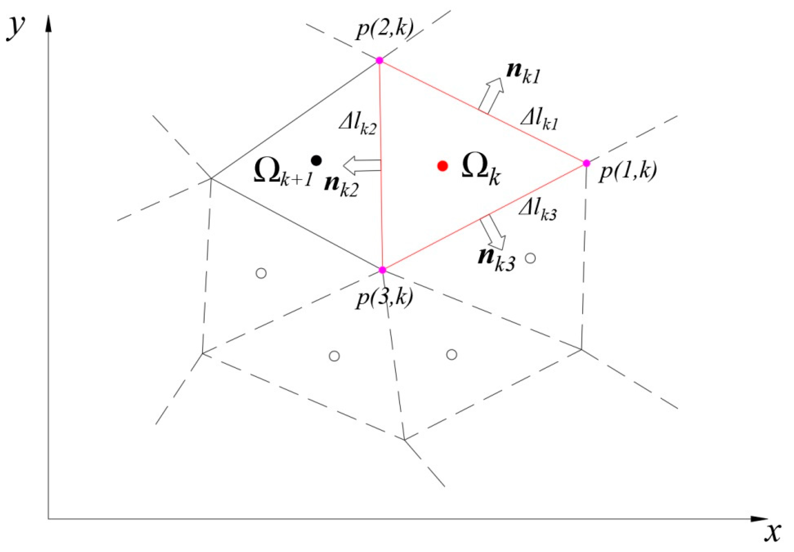
Because of the nonlinear characteristics of the SWEs, the analytical solution cannot be obtained generally but can be approximated by numerical discretization. The FVM was used to discretize the governing equation. The computational region was discretized into several points. With these points as the center, the whole computational domain was divided into several interconnected but non-overlapping control volumes. By integrating the basic equation with each control volume, a set of algebraic equations with the unknown quantity on the calculation node was obtained. A triangular mesh was used to discretize the computational domain to adapt the boundary conditions for a complex terrain. The cell-centered mode was used in the calculations, which means that the physical variables are defined in the center of the control volume [24], as shown in Figure 1.
Integration of Equation (1) over the area of the governing volume Ω, gives
In Equation (2), represents a 2D matrix.
The volume integral is transformed to a line integral along the edge of the control volume using Gauss’ formula
where is the average value of the governing cell; is the edge of the kth control volume ; is the area of each calculation cell; is the unit vector of the normal direction outside the edge.
After discretization of Equation (3), the following formula is obtained:
where is the length of each side (using triangular grids, = 1, 2, 3); and and represent the numerical fluxes and the external normal unit vector of edge . and represent the integral values of the bed and friction slope source terms in the mesh cell, respectively. The notation denotes the inner product.
Commonly used approximate Riemann solvers for the discontinuous problem include the Osher, Roe, Harten–Lax–van Leer (HLL), and HLLC schemes [25]. In the present study, the fluxes at the interface of the governing cell were estimated using the Roe scheme. The physical variables and on the interface of the left and right grid were determined to solve the Riemann discontinuity problem. The flux expression is defined as follows [26,27,28,29]:
where is the Roe average of the Jacobian matrix. The three eigenvalues of the Jacobian matrix are , while the related eigenvectors are . The left and right interface conservative form variables are and , respectively.
To improve the adaptability of the model to complicated terrain conditions, the source term reflecting the bottom topography was managed using an eigen-decomposition method, while upwind treatment was applied to balance the interface flux [30,31]:
where is the sign function. In this case, , , and . Furthermore, is the average velocity given by the Roe scheme; and ; while and are the bottom elevations of the left and right side, respectively.
An explicit scheme that discretizes the frictional slope source term was carried out to increase the stability of the computation. Eventually, the variation of the conservation after undergoing was obtained.
where is the unit matrix. Superscripts and refer to the current and updated time levels, respectively. is the globally permissible time step, which must be computed according to the CFL stability condition [32]:
where is the computational cell index, with values of 1, 2, …, . The term refer to the total number of computational grid elements; is the distance from the center of the cell (triangle centroid) to the three sides; and are the velocities in the and directions, respectively, of cell ; is the flow depth of cell . The Courant number was set to 0.8.
In the traditional GTS algorithm, the time step is equal to the minimum value for the whole computational domain and is proportional to the size of the grid elements. When the scale of each mesh element varies markedly, the uniform time-step restriction will severely reduce the efficiency of the model operation. Therefore, it is essential to explore an efficient method in which the time-step changes with the mesh size and satisfies the CFL conditions.
2.2. Local Time Stepping Scheme
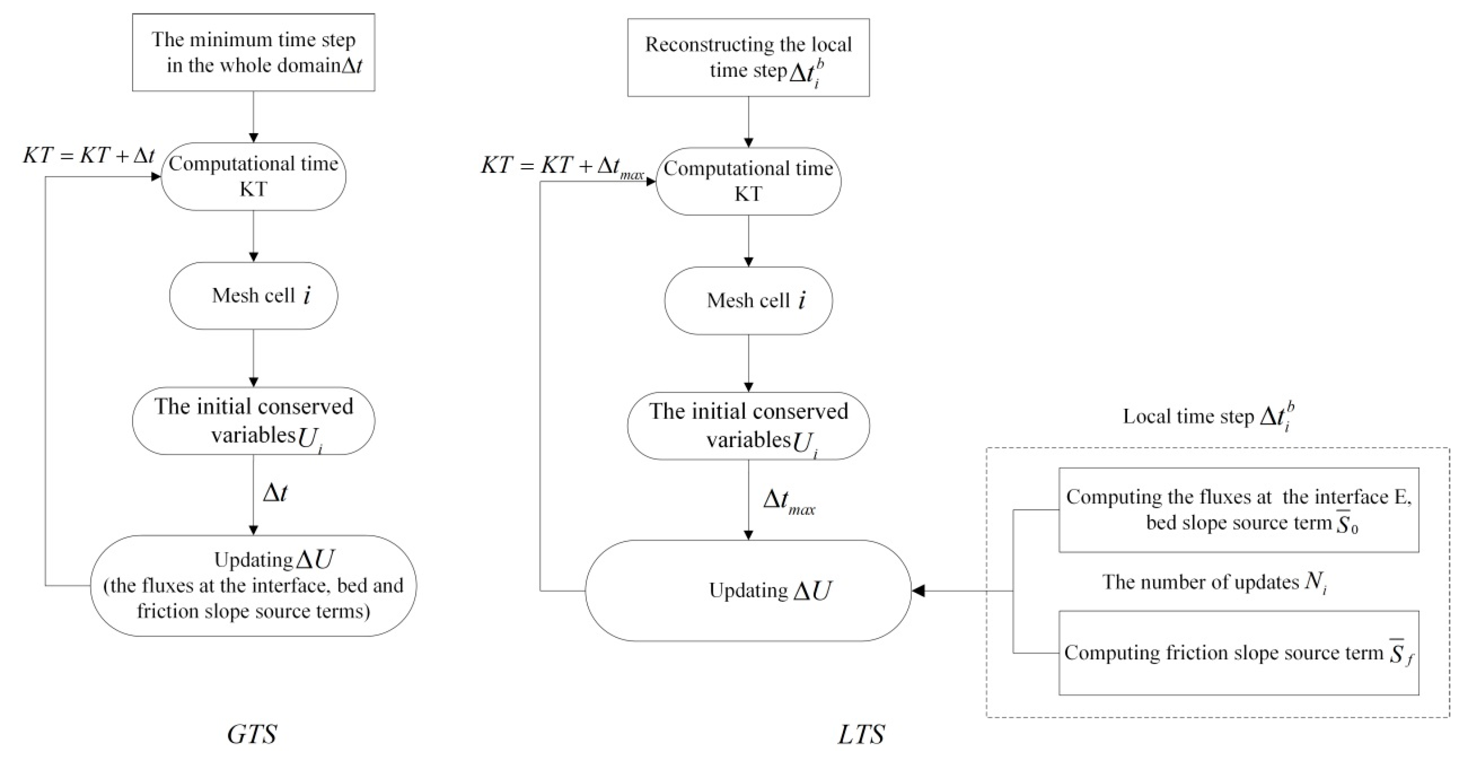
The key approach in the LTS algorithm is to advance each cell with a time step as close as possible to its maximum allowable value while satisfying the stability of the CFL condition. The algorithm reconstructs the time-step level of each cell with the aim of reducing the computational load of coarse grids, consequently saving computational time. Figure 2 compares the implementation of GTS versus LTS algorithms. The LTS algorithm differs in two aspects: reconstructing the local time step of each cell (Section 2.2.1) and updating values of the conserved variables (Section 2.2.2).
2.2.1. Reconstructing the Local Time Step of Each Cell
This procedure is defined as follows:
(1) Compute the initial time step
The of each cell satisfying the CFL condition is computed via Equation (9a):
where and are the maximum velocities in the and directions, respectively; and is the maximum water depth.
Next, calculate the minimum time step in the whole computational domain:
(2) Set an initial temporal resolution level for each cell
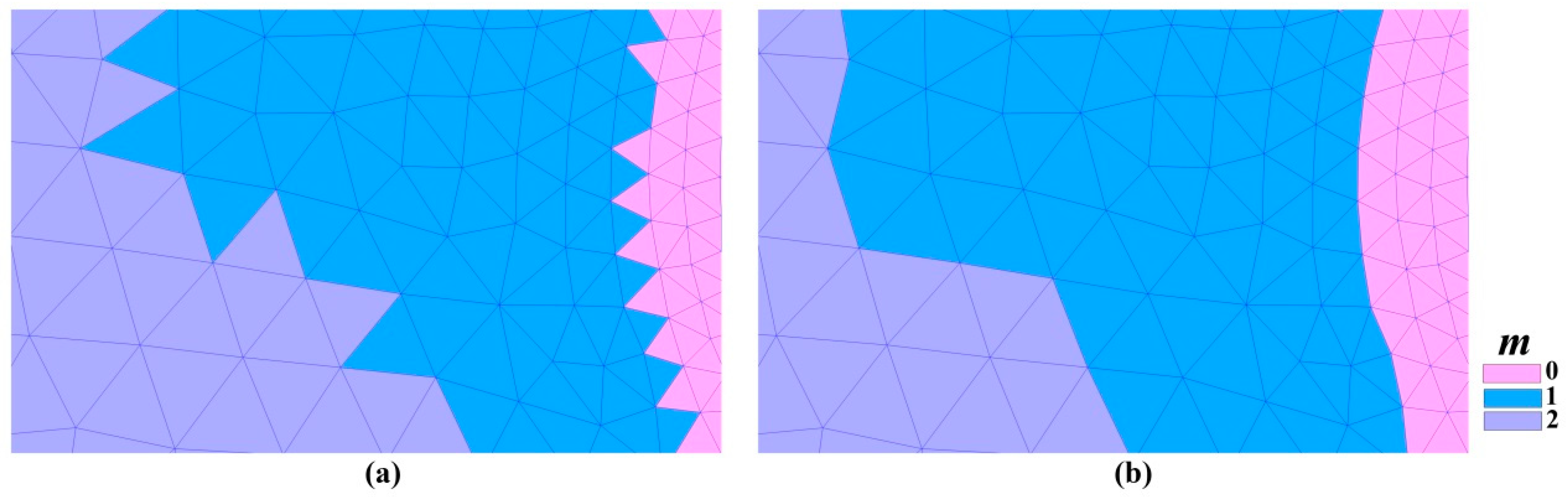
In terms of the CFL condition, the initial time step in cell is proportional to the mesh scale . Taking the minimum time step over the whole computational domain as the reference standard, a binary logarithmic function is selected as the conversion tool. Each cell is classified based on its initial time step , with the allocation of an initial time-step level , reflecting the mesh scale and having integer values of 1, 2, 4, 8, 16, 32, 64,… The initial m-level distribution map is shown in Figure 3a.
where the function of is to obtain the maximum integer that does not exceed the given number.
(3) Modify the time-step level
The initial m-level distribution calculated by Equation (10) is usually scattered and broken (see Figure 3a), especially within the transition zone between coarse and refined grids. This distribution varies dramatically because of the large difference in mesh size. Appropriate measures need to be taken to smooth the transition and to reduce mass and momentum errors in these zones related to the calculation of conserved variables at interfaces between cells with different m-levels. The initial m-levels are modified via Equation (11a), which produces a buffer zone.
where is the time-step level of the three neighboring cells of cell . The evaluation of the time-step level in cell is based on values of the neighboring cells: . If the time-step level of the current cell is larger than that of the neighboring cells, then the value will be reduced by one; otherwise, it will be retained. Thus, the difference between the m-levels of the current and neighboring cells cannot exceed one. In this way, the time-step level (see Figure 3a) is modified via Equation (11a), and the new m-level distribution is as shown in Figure 3b.
The maximum of time-step level is given by
where refers to the local time-step rank of the LTS algorithm in the computation (L = 1 represents the GTS solution). Building on the requirement of simulation accuracy, the maximum value of the different time-step level is selected according to the simulation accuracy requirements, and the restriction condition is added to Equation (11a).
In this case, the time step adopted by each calculation cell is
The maximum time step is
2.2.2. Calculation of Element Variables at the Interface
Once the local time-step level of each computation cell is reconstructed, no further cells are updated with the same time step but are instead updated with the locally allowable time step at each cell. The algorithm focuses on the convergence of the element variables at different time levels along the interface. In a maximum time step , the number of updates at each cell is calculated using
The expression for in Equation (7) is then replaced by Equation (13), in which from Equation (11c) takes the place of in each computing cell. The improved expression is as follows:
Then, Equation (13) is iterated times, and the conserved variables of each cell are updated to the same time level , from which the variables at the next time level are calculated until the calculation time terminates.
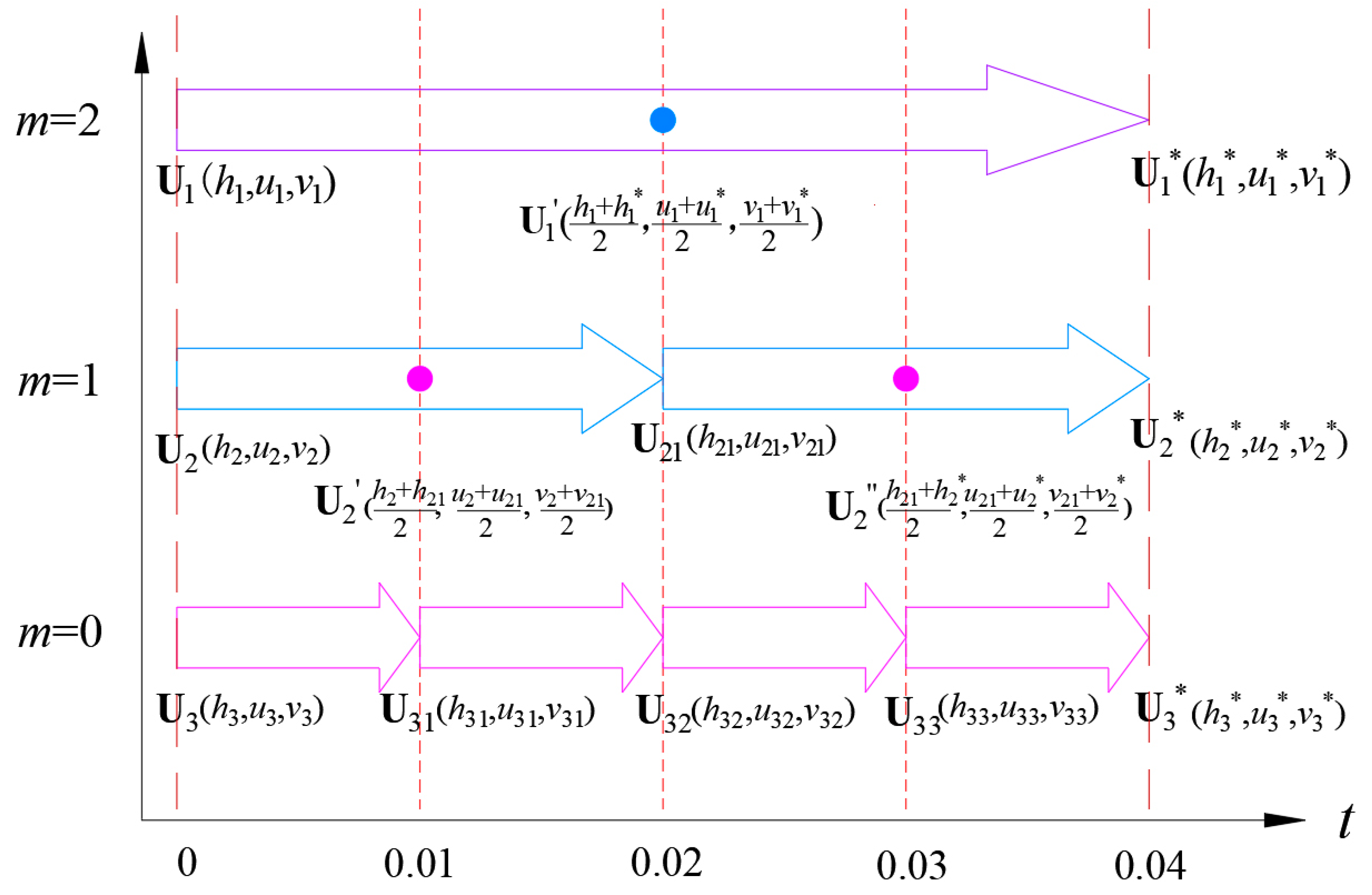
The fluxes on the interface of the governing cell are estimated from the approximate Riemann solution of the Roe scheme. However, the variable values of all cells at the current time level need to be given to confirm the and values of the adjacent states on the left and right sides of the interface. In the initial GTS model, the unified global time step can meet these requirements. In the LTS algorithm, however, when the m-level of the current and neighboring cells differ within the maximum time step , the update times are different, and time splitting occurs at the interface. In the present study, the value of the missing element variable at the interface was obtained by linear interpolation of the value of the element variable in two adjacent time layers. This is shown in Figure 4, where the maximum time-step level = 2. At the starting time of 0, we assumed that = 0.01 s. First, the element variables of the coarse grid (m = 2) were computed only once, which consumes 0.04 s. Next, the values for the intermediate meshes (m = 1) were calculated twice, costing 0.02 s for each calculation. The local time step of the coarse mesh (m = 2) at the interface is, however, 0.04 s, which suggests that the variable values at 0.02 s are missing. In the present study, the variable values were estimated approximately using the average value of the former and the latter time step (1/2 of the variable value at 0 and 0.04 s). Finally, the refined grids (m = 0) were calculated at four intervals, with time steps of 0.01 s. At 0.01 and 0.03 s, the values of the variables are absent at the interface of the cells having m = 1. The above approximation method was again used. At 0.04 s, all cell variables were updated to the same time level in preparation for the next iteration.
3. Numerical Tests
Numerical tests were carried out to verify the reliability and adaptability of the LTS strategy within a 2D hydrodynamic model, and to make a comparison between the effects of the novel LTS and the original GTS strategies on the simulation results. To quantify these differences, we used the mean-square error (MSE)
where refers to the MSE of variables (such as water depth , and velocity components and in the and directions, respectively), and the subscript L refers to the local time-step rank of the solutions.
The principle purpose of using the LTS algorithm instead of the GTS algorithm is to reduce the computing time. The relative time saving ratio and speedup ratio were used as evaluation indices of the computing efficiency for different L values.
The time saving ratio is given by
The speedup ratio is given by
where is the computation time of the GTS strategy, and is the computation time of the LTS strategy using different local time-step rank values (L).
3.1. Anti-Symmetric Dam Break Case
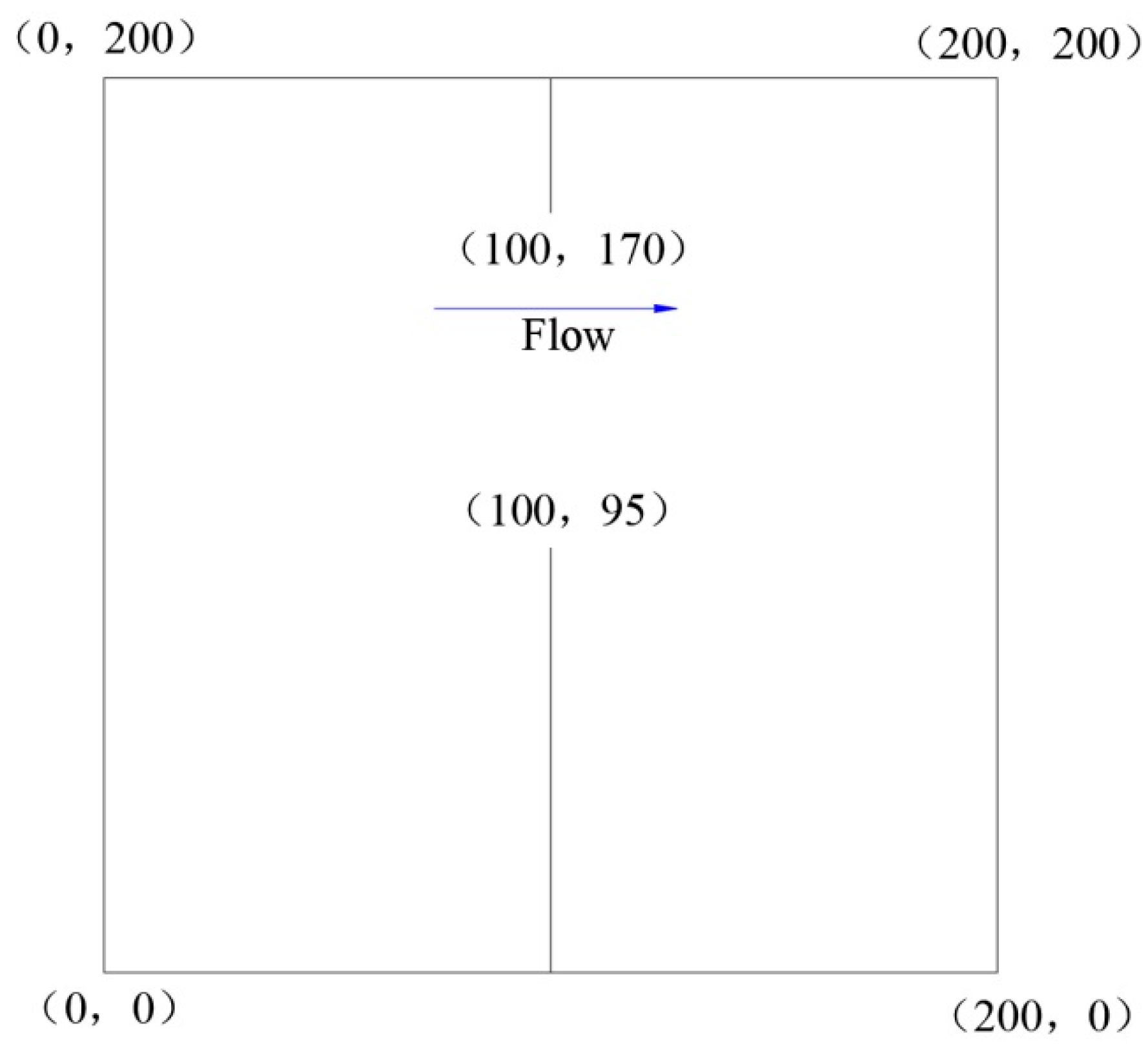
A classic verification experiment that considers the anti-symmetric square dam break case has been described by Fennema and Chaudhry [33]. The computational domain consists of a m square region with a flat bottom (bed elevation of 0 m). In this problem, the dam is assumed to fail instantaneously at a certain moment, producing an anti-symmetric breach with a width of 75 m at the center of the calculation domain, which is 95 m from the x-axis boundary. The detailed geometry of this problem is shown in Figure 5.
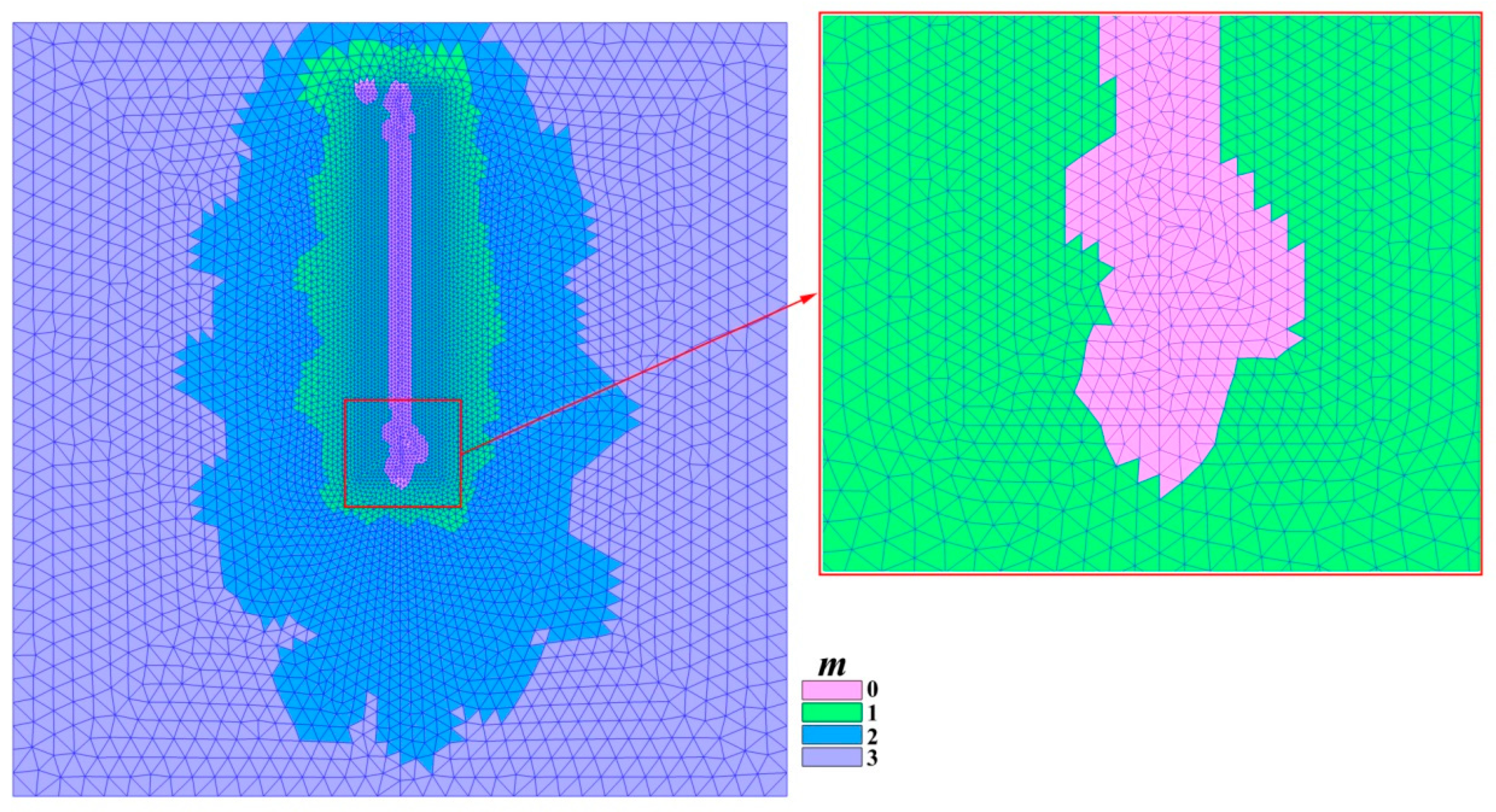
The computational domain was discretized on triangular meshes. Local mesh refinement technology was adopted near the break to accurately reflect the important flow regions while controlling the number of grids. The spatial resolution level varied from 6 to 1 m, with a refined area of 5%. A total of 13,338 computing cells were generated. The LTS algorithm was applied to shorten the computing time and improve the calculation efficiency. The m-level distribution of the LTS strategy is presented in Figure 6. The simulation duration was = 160 s. At the initial moment, upstream water depth was set to 10.0 m, while downstream water depth was assumed to be 5.0 m. Manning’s roughness coefficient was set to 0.03 [34].
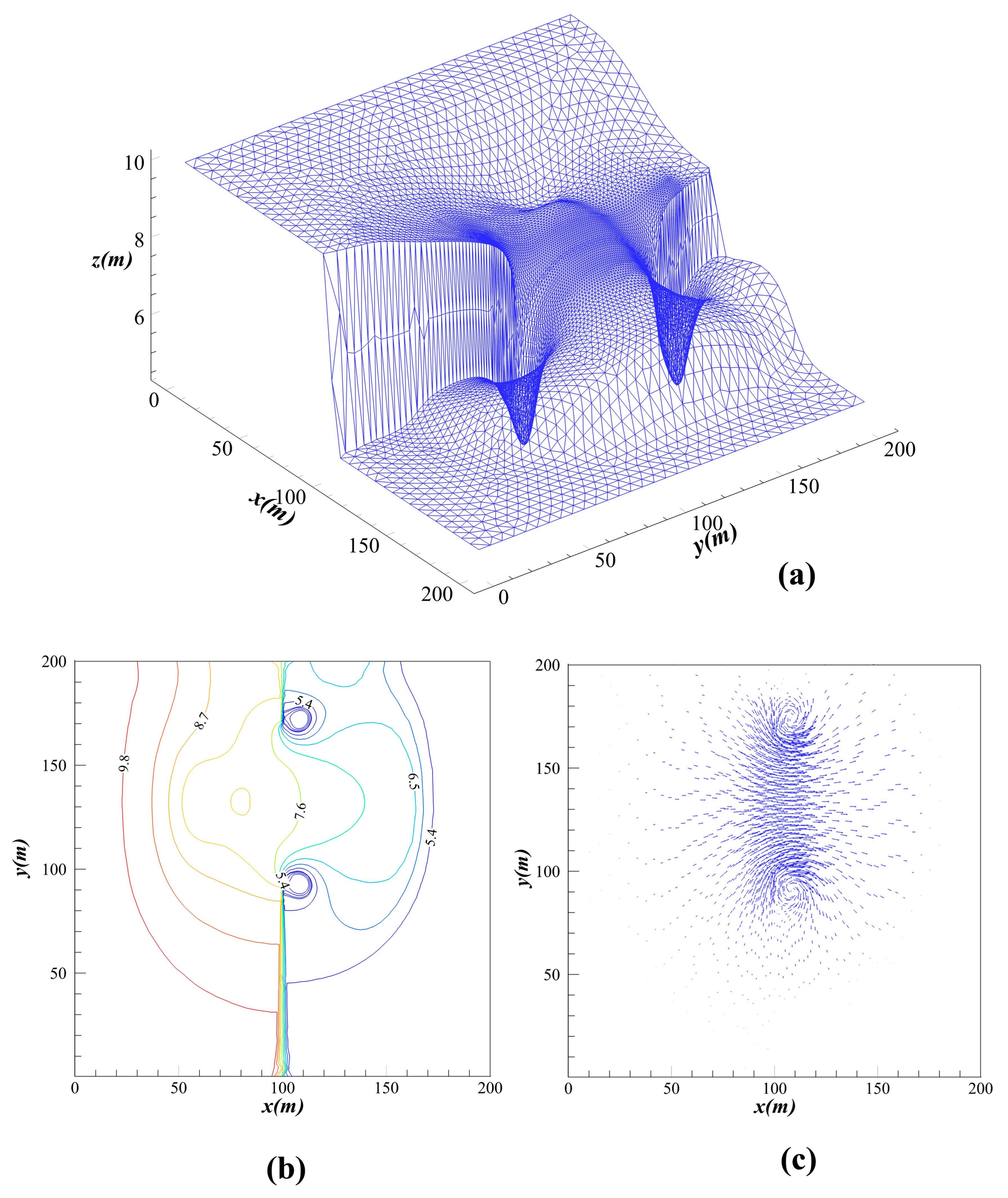
Before making a quantitative analysis of the MSE generated by the LTS strategy, it is useful to verify the validity of the GTS scheme applied to the original model. The numerical solution results at t = 7.2 s were obtained using the GTS strategy; the resulting water surface profiles are shown in Figure 7a, contours of water depth in Figure 7b, and velocity vector distribution in Figure 7c. These results effectively simulated the dam break waves and are consistent with previous research results [34,35,36].
Table 1 shows the MSE of water depth , as well as velocity components and along the and directions, respectively, of the simulation results. As the value of the local time-step rank L increased, the MSE increased accordingly. Both precision and efficiency are important when performing hydrodynamic numerical simulations. By reducing the value of L, the calculation efficiency can be improved when levels of high accuracy are reached. This observation agrees well with the research results of Hu et al. [37]. In the present study, the error of the solution using the LTS algorithm was within the 10−3 to 10−2 range. At the beginning of the calculation, the total water volume was 3 × 10⁵ m3. When the value of L was 2, 3, and 4, the relative error of the water volume was 0.0017%, 0.0019%, and 0.0045%, respectively, which indicates that the simulation meets the accuracy and conservation of water volume requirements.
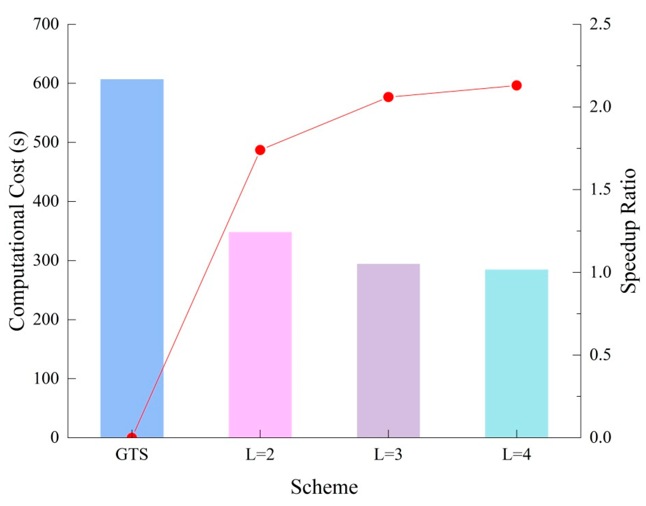
Table 2 shows the computing time, time-saving ratio, and speedup ratio for different values of L. The simulation time of the dam break was 160 s. A time saving of 40% to 50% was achieved using the LTS algorithm in the numerical experiment of the anti-symmetric square dam break. For L = 4, a speedup ratio of 2.1 was achieved.
This clearly shows that the calculation efficiency of the numerical simulation of the anti-symmetric square dam break is improved using the LTS technique (Figure 8). As the value of L increased, the speedup ratio also increased, thus shortening the model operation.
3.2. Non-Flat Bottom Dam Break Case
In this test case, the length of the rectangular channel was 75 m, and its width was 30 m. Three obstacles were placed on the bottom of the rectangular channel. Two obstacles had a radius of 6.5 m and a height of 1 m, and one had a radius of 8.6 m and a height of 2 m. The elevation expression is defined as follows:
Local mesh refinement was applied with a spatial resolution level varying from 0.5 to 3 m. The grid generation results are shown in Figure 9. The total number of grid cells for the region was 6848. In the calculation, a solid wall boundary condition was adopted. Manning’s roughness coefficient was set to 0.018 [30]. The water depth for 16 m in the computational domain was set to 2 m and was assumed to be 0 m elsewhere. The variation of the ground level is shown in Figure 10a. In the GTS scheme, the time step was 0.005 s, the initial total water volume was 959.841 m3, and the final water volume was 959.978 m3. The relative error was 0.01%, which is within the discrete error range. The model dealt well with wetting and drying fronts over the complex terrain, satisfied computational stability, and conservation of water volume requirements, and provided results that were consistent with previous experimental results [38,39].
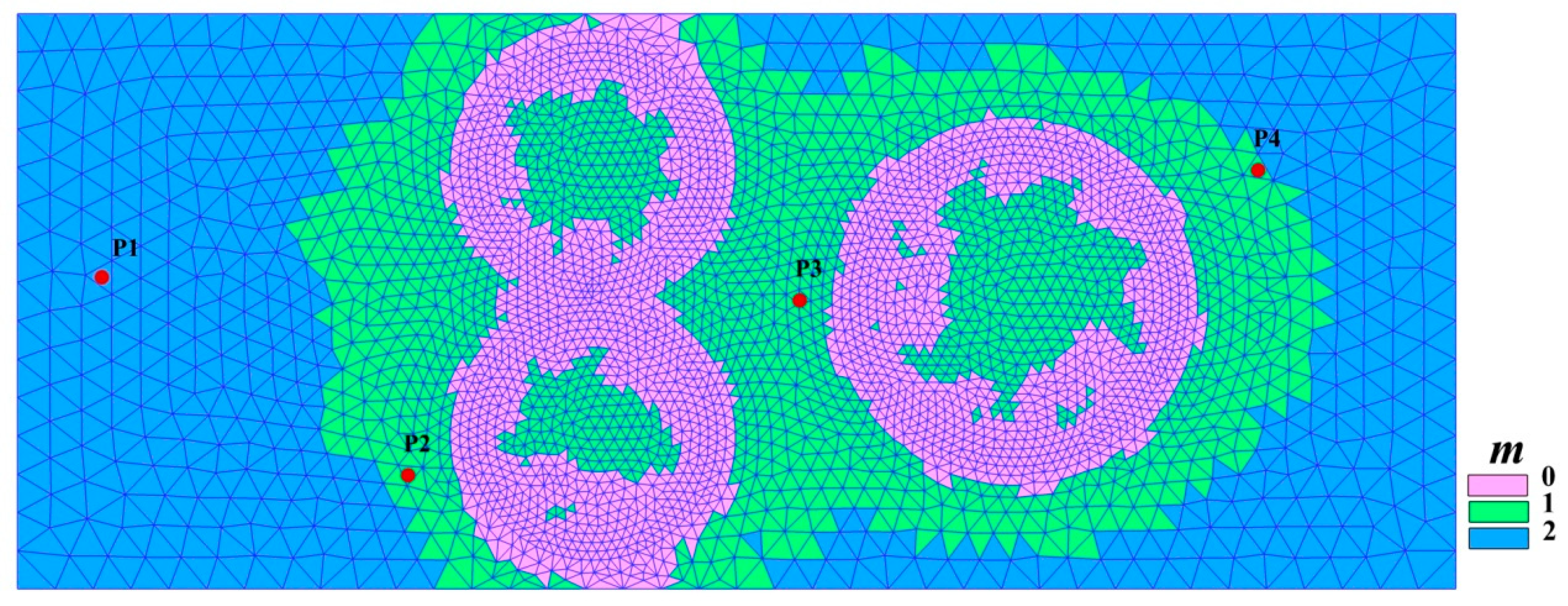
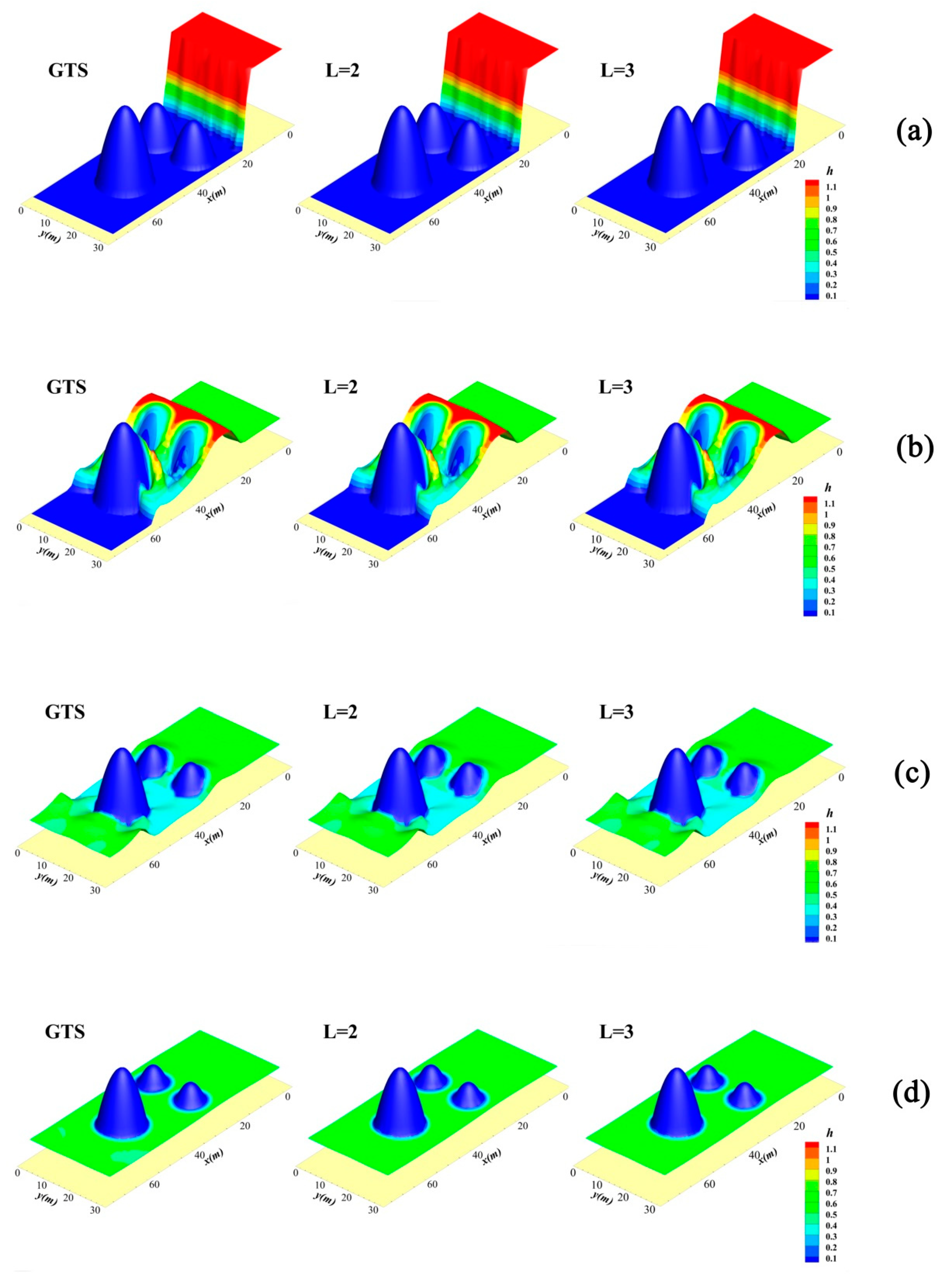
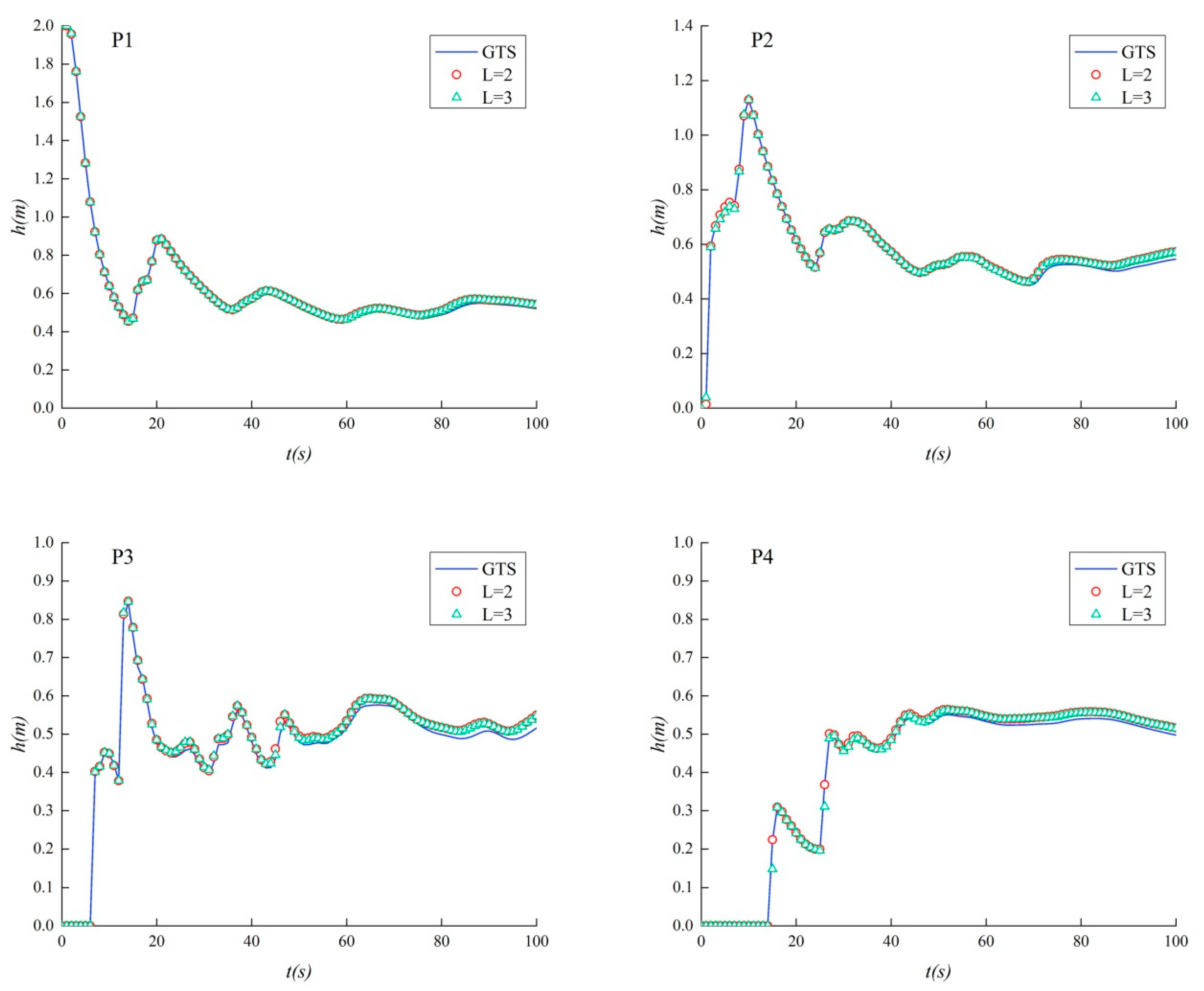
The distribution of m-values obtained by applying the LTS strategy is shown in Figure 9. The maximum time-step level is 2. The simulation of the dam break water flow was modeled for = 100 s. The inundation related to the dam break is shown in Figure 10. To observe the influence of the LTS algorithm on the simulation results, four bathymetric measuring points were arranged (see Figure 9 for the location of the measuring points). Figure 11 provides a comparison of water depths generated by the LTS algorithm and the classical algorithm during the process of the dam break. A visual inspection indicates that the simulated water depths from the two algorithms are essentially the same. Thus, the LTS technique improves the efficiency of calculation without any reduction in accuracy.
According to the statistical results for this simulation (shown in Table 3), adopting the LTS technology in the numerical experiment of the non-flat bottom dam break created a saving of up to 26% in computation time, and a speedup ratio of 1.3, without compromising the solution accuracy. The best result was obtained for L = 3, which reduced the computational cost and improved the calculation efficiency.
3.3. Navigable Flow Simulation Case
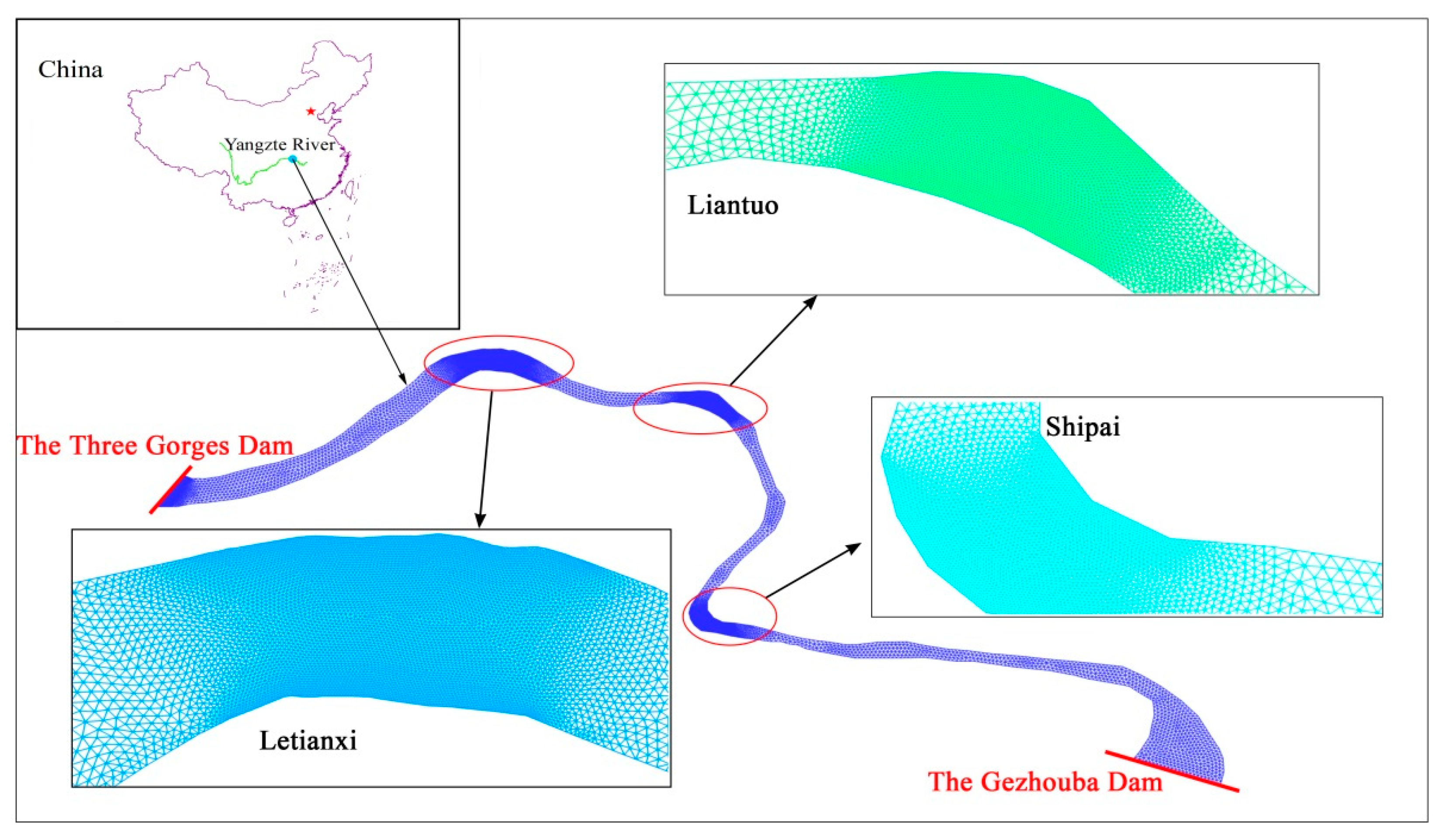
There are several noticeable perilous waterways between the Three Gorges Dam and the Gezhouba Dam. The river section is about 38 km long [40,41]. Bed elevations measured in October 2008 provided by the Three Gorges Navigation Authority were used as the initial bed topography. In the present study, the three segments with the highest risk to shipping (the Letianxi, Liantuo, and Shipai riverways), and the outlet of the Three Gorges Reservoir are adopted for local mesh refinement. The spatial resolution level ranged from 10 to 100 m, and 36,297 cells and 19,011 nodes were generated. The results of the grid generation and refined areas are shown in Figure 12.
The LTS algorithm was applied to the numerical simulation of the navigable flow of the waterway. The results are provided in Table 4. The maximum time-step level ( = 4) and the minimum time step ( = 0.03 s) were calculated for the whole computational domain. The simulation duration was set to = 4 h. The absolute deviation in the water level between the calculated and measured values was 0.06 to 0.07 m, and the relative deviation in flow velocity was between −3.8% and 4.6%. There is no significant difference between the LTS and GTS algorithm simulation results for water level and flow velocity. The mass errors are non-negligible for a large computational area and a long simulation. This was addressed by adopting a smaller maximum time-step level . The obvious acceleration effect that this provides in the real application ensures that accuracy requirements are met. It is clear that the LTS algorithm has provided obvious improvements in the execution time without compromising the solution accuracy. This is of practical value and importance in navigation.
4. Discussion
4.1. The Influence of the Proportion of Refined Mesh on the Acceleration Effect
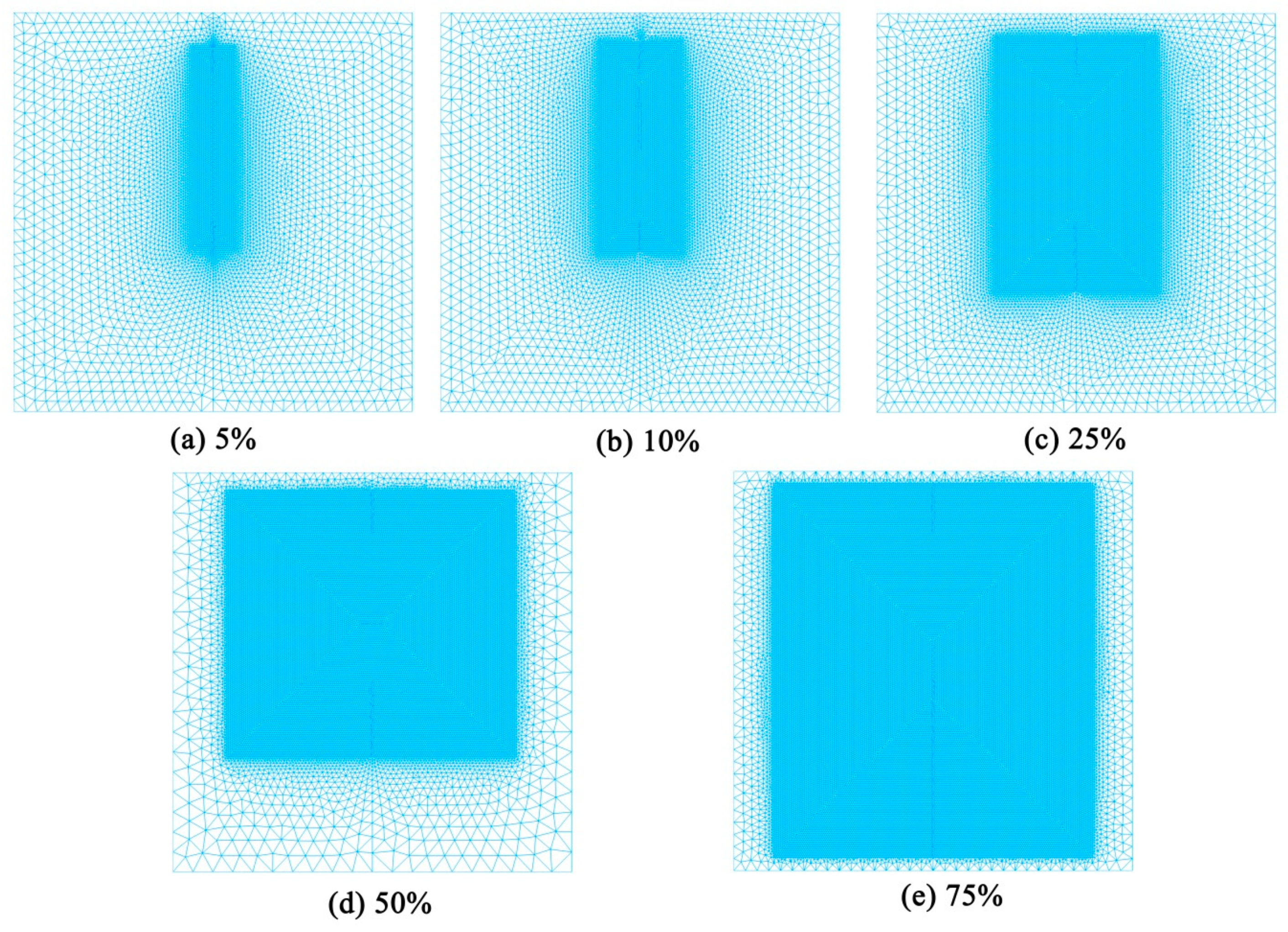
In the anti-symmetric dam break case, the 75-m breach was used as the core area in which to analyze the acceleration effect of the LTS algorithm. In this area, we set the refined area to different proportions of the total area (4 hm2). The spatial resolution level varied from 1 to 6 m, with a minimum resolution close to the breach of 1 m, surrounded by a smooth transition up to a maximum resolution of 6 m in the outer domain. The mesh generation results for the refined areas for various proportions in the anti-symmetric dam break case is shown in Figure 13. The numerical simulation was performed for refined areas of 5%, 10%, 25%, 50%, and 75%. The impact of increasing the local refinement area on the acceleration effect was analyzed for a time-step level of m = 0 in the refinement area, m = 2 in the coarse grid area, and m = 1 in the buffer zone.
The duration of the dam break was kept at 160 s. Table 5 shows the number of generated grids, computational cost, speedup ratio, and time-saving ratio for different refined area proportions. As the refined area was increased, the total number of meshes generated by partitioning increased. The grid number increased from 13,338 at 0.2 hm2 to 73,306 at 3 hm2, which represents an increase by a factor of 5.5. The operating time of the model rose from 608 to 3394 s, which represents an increase by a factor of 5.6. The number of grids is a key factor determining the overhead of computing. There is a direct positive correlation between the number of grids and computing overheads.
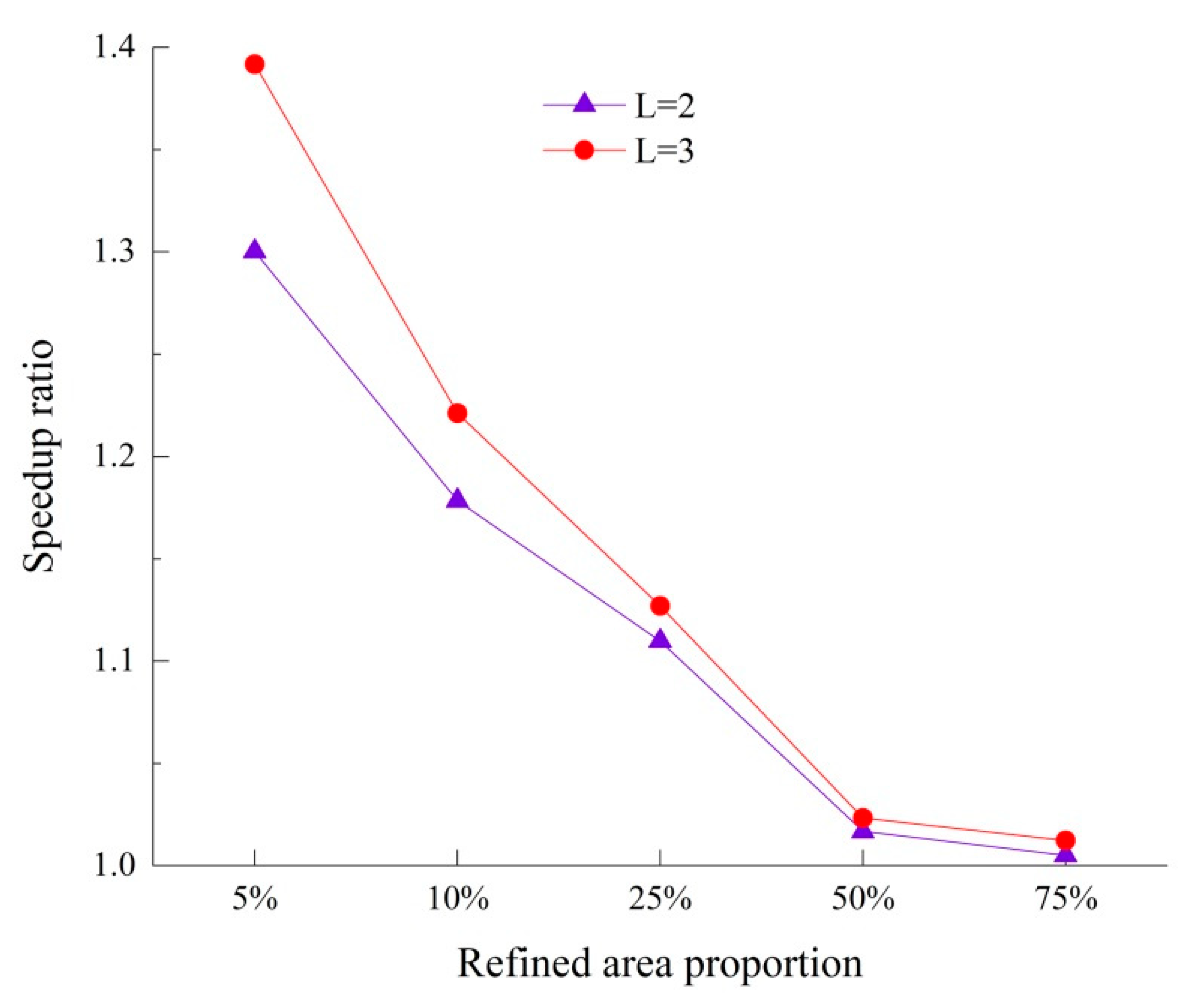
The speedup ratio was strongly affected by the ratio of the locally refined area to the total area. As the proportion of the refined area increased, the speedup ratio obtained by the LTS algorithm diminished, reducing the acceleration effect. When L = 3, the speedup ratio decreased from 1.39 times to 1.01 times; when the refined area was increased from 5% to 75%, there was scarcely any improvement in computational efficiency at high proportions of refined area. These patterns occurred because a high proportion of refined area brings about an unreasonable number of refined grids (with a local time-step level, m = 0), which reduces the number of coarse grids (m = 1, 2) that help optimize the operation. This suggests that little improvement is gained by implementing the LTS algorithm in cases that have a high proportion of refined grids. Conversely, when refined grids account for a small proportion of the total number of grids, the LTS algorithm can markedly shorten the computing time and achieve an excellent acceleration effect. Furthermore, the results in Figure 14 suggest that L has an influence on the calculation efficiency. The acceleration ratio increased as L increased.
4.2. The Impact of the Different Scale of the Mesh on Acceleration Effect
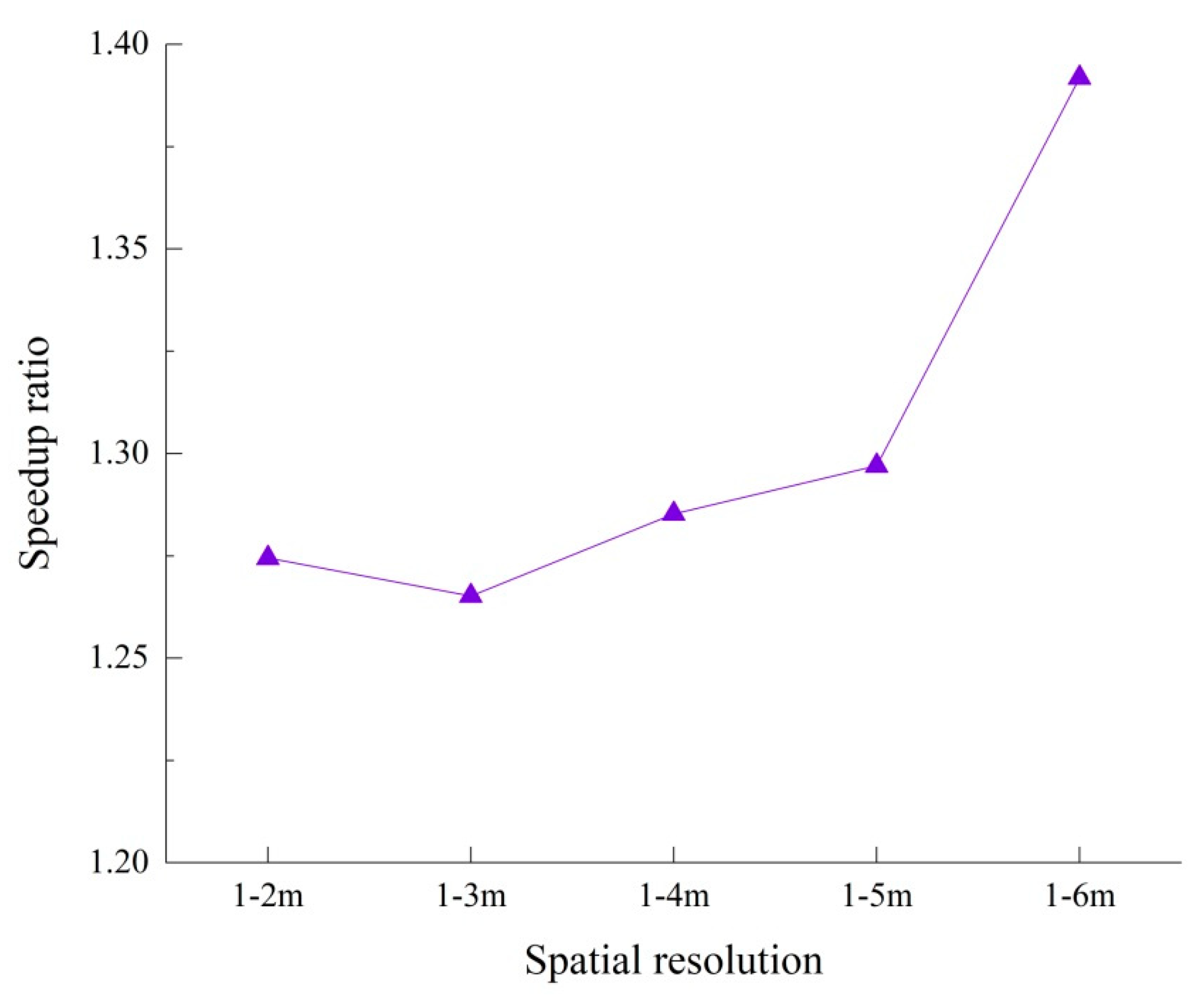
In the case study of the anti-symmetric dam break, the test was carried out using a refinement of 5% of the breach area, as shown in Figure 13a. A grid discretization method was employed to analyze the influence of using different grid scales on the acceleration effect while using the LTS algorithm. The refined grid had a minimum spatial step of 1 m in the burst section, while the coarse grids had spatial steps of 2, 3, 4, 5, and 6 m. The computational results are shown in Table 6 and Figure 15. These results indicate that the speedup ratio improves with the increasing differences in grid resolution. The CFL condition of Equation (9a) shows that the time step of the mesh is positively correlated with the mesh scale difference. As the difference between the maximum and minimum scales of the grids increases, the maximum time-step level becomes higher, and a larger L can be adopted. In this test, once the spatial step of the coarse grid was 4, 5, and 6 m, it was possible to set the L value to 3, while the other two conditions were only subdivided into two grades. This explains why greater grid diversity leads to a higher speedup ratio.
5. Conclusions
Improvements in the computational efficiency of the 2D hydrodynamic model have a significant bearing on its engineering applications. In the present study, an improved 2D shallow-water dynamic model applying an LTS algorithm was established using an FVM on a triangular mesh. Results from simulation and analysis of three canonical test cases show that the LTS scheme has a satisfactory ability for adapting real complex applications and long simulations while meeting the required accuracy. The following conclusions were drawn:
- (1)
- Based on the FVM for unstructured grids, an LTS algorithm was implemented that improved the computational efficiency of the model, while satisfying water conservation conditions. In the anti-symmetric dam break case, a speedup ratio of 2.1 was achieved, which saved 53% in execution time. The speedup ratio of the non-flat bottom dam break case was 1.3, which represented a shortening of 26% in the calculation time. The numerical simulation of the navigable flow of the river reach between the Three Gorges and Gezhouba Dams achieved a speedup ratio of 1.9, which represented a saving of 49% in modeling time.
- (2)
- The proportions of coarse to refined meshes on the acceleration effect of the LTS algorithm were noticeable. It was evident that a higher speedup ratio was obtained when the proportion of the refined mesh was minimized. When the proportion of the refined mesh was high, the acceleration effect was not significant. It is clear that the LTS algorithm is best suited to situations in which refinement is only required in small regions.
- (3)
- When using the LTS algorithm on non-uniform unstructured grids, the larger the grid scale difference, the more obvious the grid layering became. This led to increased acceleration effects. However, computational accuracy was slightly impaired by excessive differences in grid mesh size.
Author Contributions
Conceptualization, S.Z. and X.Y.; Methodology, S.Z. and X.Y.; Software, X.Y., W.A. and W.L.; Validation, S.Z., X.Y., W.A. and W.L.; Formal Analysis, S.Z.; Investigation, X.Y. and W.A.; Resources, S.Z.; Data Curation, X.Y. and W.A.; Writing—Original Draft Preparation, X.Y.; Writing—Review & Editing, S.Z.; Supervision, S.Z. All authors have read and agreed to the published version of the manuscript.
Funding
This study was supported by the National Natural Science Foundation of China (51979105, 51722901).
Acknowledgments
The authors thank Trudi Semeniuk and Paul Seward from Liwen Bianji, Edanz Editing China (www.liwenbianji.cn/ac), for editing the English text of drafts of this manuscript.
Conflicts of Interest
The authors declare no conflict of interest.
References
- Wang, Z.; Gang, Y.; Jin, S. Numerical modeling of 2D shallow water flow with complicated geometry and topography. J. Hydraul. Eng. 2005, 36, 439–444. (In Chinese) [Google Scholar]
- Jin, H.; Jespersen, D.; Mehrotra, P.; Biswas, R.; Huang, L.; Chapman, B. High performance computing using MPI and OpenMP on multi-core parallel systems. Parallel Comput. 2011, 37, 562–575. [Google Scholar] [CrossRef]
- Zhang, S.; Xia, Z.; Yuan, R.; Jiang, X. Parallel computation of a dam-break flow model using OpenMP on a multi-core computer. J. Hydrol. 2014, 512, 126–133. [Google Scholar] [CrossRef]
- Vacondio, R.; Dal Palù, A.; Ferrari, A.; Mignosa, P.; Aureli, F.; Dazzi, S. A non-uniform efficient grid type for GPU-parallel Shallow Water Equations models. Environ. Model. Softw. 2017, 88, 119–137. [Google Scholar] [CrossRef]
- Dawson, C. High Resolution Schemes For Conservation Laws With Locally Varying Time Steps. SIAM J. Sci. Comput. 2000, 22, 2256–2281. [Google Scholar] [CrossRef] [Green Version]
- Sanders, B.F. Integration of a shallow water model with a local time step. J. Hydraul. Res. 2008, 46, 466–475. [Google Scholar] [CrossRef]
- Kesserwani, G.; Liang, Q. RKDG2 shallow-water solver on non-uniform grids with local time steps: Application to 1D and 2D hydrodynamics. Appl. Math. Model. 2015, 39, 1317–1340. [Google Scholar] [CrossRef]
- Caboussat, A.; Boyaval, S.; Masserey, A. On the modeling and simulation of non-hydrostatic dam break flows. Comput. Vis. Sci. 2011, 14, 401–417. [Google Scholar] [CrossRef] [Green Version]
- Li, D.; Zeng, Q.; Feng, H. A P-adaptive Discontinuous Galerkin Method Using Local Time-stepping Strategy Applied to the Shallow Water Equations. J. Inf. Comput. Sci. 2013, 10, 2199–2210. [Google Scholar] [CrossRef]
- Tirupathi, S.; Hesthaven, J.S.; Liang, Y.; Parmentier, M. Multilevel and local time-stepping discontinuous Galerkin methods for magma dynamics. Comput. Geosci. 2015, 19, 965–978. [Google Scholar] [CrossRef] [Green Version]
- Zhou, W.; Ouyang, J.; Wang, X.; Su, J.; Yang, B. Numerical simulation of viscoelastic fluid flows using a robust FVM framework on triangular grid. J. Non-Newton. Fluid Mech. 2016, 236, 18–34. [Google Scholar] [CrossRef]
- Cheng, L.; Hu, C. An adaptive multi-moment FVM approach for incompressible flows. J. Comput. Phys. 2018, 359, 239–262. [Google Scholar]
- Osher, S.; Sanders, R. Numerical approximations to nonlinear conservation laws with locally varying time and space grids. Math. Comput. 1983, 41, 321–336. [Google Scholar] [CrossRef]
- Tan, Z.; Huang, Y. An Adaptive Grid Method with Local Time Stepping for One Dimensional Conservation Laws. Nat. Sci. J. Xiangtan Univ. 2003, 25, 110–116. (In Chinese) [Google Scholar]
- Crossley, A.J.; Wright, N.G.; Whitlow, C.D. Local time stepping for modeling open channel flows. J. Hydraul. Eng. 2003, 129, 455–462. [Google Scholar] [CrossRef]
- Crossley, A.J.; Wright, N.G. Time accurate local time stepping for the unsteady shallow water equations. Int. J. Numer. Methods Fluids 2005, 48, 775–799. [Google Scholar] [CrossRef]
- Dazzi, S.; Maranzoni, A.; Mignosa, P. Local time stepping applied to mixed flow modelling. J. Hydraul. Res. 2016, 54, 145–157. [Google Scholar] [CrossRef]
- Dazzi, S.; Vacondio, R.; Dal Palù, A.; Mignosa, P. A local time stepping algorithm for GPU-accelerated 2D shallow water models. Adv. Water Resour. 2018, 111, 274–288. [Google Scholar] [CrossRef]
- Wu, D.; Yu, X.; Xu, Y. A Discontinuous Galerkin Method with Local Time Stepping for Euler Equations. Chin. J. Comput. Phys. 2016, 28, 1–9. (In Chinese) [Google Scholar]
- Trahan, C.J.; Dawson, C. Local time-stepping in Runge–Kutta discontinuous Galerkin finite element methods applied to the shallow-water equations. Comput. Methods Appl. Mech. Eng. 2012, 217–220, 139–152. [Google Scholar] [CrossRef]
- Hu, P.; Lei, Y.; Han, J.; Cao, Z.; Liu, H.; He, Z. Computationally efficient modeling of hydro–sediment-morphodynamic processes using a hybrid local time step/global maximum time step. Adv. Water Resour. 2019, 127, 26–38. [Google Scholar] [CrossRef]
- Baldauf, M. Local time stepping for a mass-consistent and time split advection scheme. R. Meteorol. Soc. 2019, 145, 337–346. [Google Scholar] [CrossRef] [Green Version]
- Toro, E.F. Shock-Capturing Methods for Free-Surface Shallow Flows; John Wiley: Hoboken, NJ, USA, 2001. [Google Scholar]
- Thompson, J.F.; Warsi, Z.U.A.; Mastin, C.W. Numerical Grid Generation; North Holland: New York, NY, USA, 1985; Chapter 6; pp. 129–165. [Google Scholar]
- Pan, C. Advanced in numerical simulation of discontinuous shallow water flows. Adv. Sci. Technol. Water Resour. 2010, 30, 77–84. (In Chinese) [Google Scholar]
- Zhang, D.; Li, D.; Wang, X. Numerical modeling of dam-break water flow with wetting and drying change based on unstructured grids. J. Hydroelectr. Eng. 2008, 27, 98–102. (In Chinese) [Google Scholar]
- Murillo, J.; García-Navarro, P. Wave Riemann description of friction terms in unsteady shallow flows: Application to water and mud/debris floods. J. Comput. Phys. 2012, 231, 1963–2001. [Google Scholar] [CrossRef]
- Vacondio, R.; Dal Palù, A.; Mignosa, P. GPU-enhanced Finite Volume Shallow Water solver for fast flood simulations. Environ. Model. Softw. 2014, 57, 60–75. [Google Scholar] [CrossRef]
- Fernández-Pato, J.; Morales-Hernández, M.; García-Navarro, P. Implicit finite volume simulation of 2D shallow water flows in flexible meshes. Comput. Methods Appl. Mech. Eng. 2018, 328, 1–25. [Google Scholar] [CrossRef] [Green Version]
- Brufau, P.; Vázquez-Cendón, M.E.; García-Navarro, P. A numerical model for the flooding and drying of irregular domains. Int. J. Numer. Methods Fluids 2002, 39, 247–275. [Google Scholar] [CrossRef]
- Lv, B.; Jin, S.; Ai, C. Well-balanced Roe-type scheme for 2D shallow water flow using unstructured grids. Hydro-Sci. Eng. 2010, 2, 39–44. (In Chinese) [Google Scholar]
- Toro, E.F. Riemann Solvers and Numerical Methods for Fluid Dynamics; Springer: Berlin/Heidelberg, Germany, 2013; pp. 87–114. [Google Scholar]
- Fennema, R.J.; Chaudhry, M.H. Explicit methods for 2-D transient free surface flows. J. Hydraul. Eng. 1990, 116, 1013–1034. [Google Scholar] [CrossRef]
- Wang, D. Computational Hydraulics: Theory and Application; Science Press: Beijing, China, 2011. (In Chinese) [Google Scholar]
- Liu, H.; Zhou, J.G.; Burrows, R. Lattice Boltzmann simulations of the transient shallow water flows. Adv. Water Resour. 2010, 33, 387–396. [Google Scholar] [CrossRef]
- Baghlani, A. Simulation of dam-break problem by a robust flux-vector splitting approach in Cartesian grid. Sci. Iran. 2011, 18, 1061–1068. [Google Scholar] [CrossRef]
- Hu, P.; Han, J.; Lei, Y. Coupled modeling of sediment-laden flows based on local-time-step approach. J. Zhejiang Univ. (Eng. Sci.) 2019, 53, 743–752. (In Chinese) [Google Scholar]
- Kawahara, M.; Umetsu, T. Finite element method for moving boundary problems in river flow. Int. J. Numer. Methods Fluids 1986, 6, 365–386. [Google Scholar] [CrossRef]
- Zhang, H.; Zhou, J.; Bi, S.; Song, L.X. Two-dimensional shallow hydrodynamic model based on adaptive structured grid. Chin. J. Hydrodyn. 2012, 27, 667–678. (In Chinese) [Google Scholar]
- Yan, W.; Zhou, R.; Cheng, Z.; Yang, W.; Lu, H. Adaptation of fleets to the navigation discharge in the waterway between Three Gorges Project and Gezhouba Hydroproject. J. Yangtze River Sci. Res. Inst. 2013, 6, 33–37. (In Chinese) [Google Scholar]
- Zhang, S.; Jing, Z.; Li, W.; Wang, L.; Liu, D.; Wang, T. Navigation risk assessment method based on flow conditions: A case study of the river reach between the Three Gorges Dam and the Gezhouba Dam. Ocean Eng. 2019, 175, 71–79. [Google Scholar] [CrossRef]
Figure 1.
Schematic diagram of the two-dimensional model with finite volume discretization: physical variables are defined at the grid center, where is the kth control volume; is the unit normal vector; is a grid point; and is the length of a side.
Figure 1.
Schematic diagram of the two-dimensional model with finite volume discretization: physical variables are defined at the grid center, where is the kth control volume; is the unit normal vector; is a grid point; and is the length of a side.

Figure 2.
Flow diagram showing global time stepping (GTS) and local time stepping (LTS) algorithms. In the GTS scheme, each cell is updated with the same time step , while in the LTS scheme, a locally allowable maximum time step () is used for updating variables in each cell.
Figure 2.
Flow diagram showing global time stepping (GTS) and local time stepping (LTS) algorithms. In the GTS scheme, each cell is updated with the same time step , while in the LTS scheme, a locally allowable maximum time step () is used for updating variables in each cell.

Figure 3.
Example of the m-level assignment to each cell in the unstructured grid. (a) Distribution showing initial values assigned by Equation (10); (b) distribution after being modified by Equation (11a), with the reassignment of buffer zone values based on neighboring cells values.
Figure 3.
Example of the m-level assignment to each cell in the unstructured grid. (a) Distribution showing initial values assigned by Equation (10); (b) distribution after being modified by Equation (11a), with the reassignment of buffer zone values based on neighboring cells values.

Figure 4.
Sketch showing the calculation of element variables at an interface: the variable refers to the water depth , and the velocity components and in the and directions, respectively. Within a maximum time step of = 0.04 s, the coarse mesh areas (time-step level, m = 2) were updated only once. The value of at 0 s was updated to after 0.04 s. The blank value at 0.02 s was estimated using the average of the values at the former and the latter time-step level, giving . Immediately following this, the intermediate grids (m = 1) were updated twice over this maximum time step. The values of variables at 0.01 and 0.03 s were similarly approximated. Finally, the refined mesh grids (m = 0) were updated four times over this interval. All variables were ultimately updated to 0.04 s, which allowed the next time step to be performed.

Figure 5.
Sketch showing the plane geometry of an anti-symmetric dam break, with the breach occurring in the center.
Figure 5.
Sketch showing the plane geometry of an anti-symmetric dam break, with the breach occurring in the center.

Figure 6.
Details of the non-uniform unstructured meshes and time-step level (m-level) distribution for the anti-symmetric dam break case.
Figure 6.
Details of the non-uniform unstructured meshes and time-step level (m-level) distribution for the anti-symmetric dam break case.

Figure 7.
Results of the simulation using the global time stepping strategy at dam break (t = 7.2 s). (a) Three-dimensional visualization of the water surface; (b) contour plot of water depth; (c) velocity vector distribution.
Figure 7.
Results of the simulation using the global time stepping strategy at dam break (t = 7.2 s). (a) Three-dimensional visualization of the water surface; (b) contour plot of water depth; (c) velocity vector distribution.

Figure 8.
Computational cost (s) and speedup ratios for different local time-step rank values (L) for the anti-symmetric dam break case. As the value of L increases, the computational cost decreases and the speedup ratio increases.
Figure 8.
Computational cost (s) and speedup ratios for different local time-step rank values (L) for the anti-symmetric dam break case. As the value of L increases, the computational cost decreases and the speedup ratio increases.

Figure 9.
Details of the non-uniform unstructured meshes, time-step level (m-level) distribution, and bathymetric point arrangement for the non-flat bottom dam break case.
Figure 9.
Details of the non-uniform unstructured meshes, time-step level (m-level) distribution, and bathymetric point arrangement for the non-flat bottom dam break case.

Figure 10.
Three-dimensional visualization of the inundation process at various time points following the dam break. (a) t = 0 s; (b) t = 10 s; (c) t = 30 s; (d) t = 100 s. (GTS: global time stepping strategy, while L is the time-step rank value in the local time stepping strategy).
Figure 10.
Three-dimensional visualization of the inundation process at various time points following the dam break. (a) t = 0 s; (b) t = 10 s; (c) t = 30 s; (d) t = 100 s. (GTS: global time stepping strategy, while L is the time-step rank value in the local time stepping strategy).

Figure 11.
Comparison of water levels at different local time-step rank values (L) for the non-flat bottom dam break case (GTS: global time stepping strategy).
Figure 11.
Comparison of water levels at different local time-step rank values (L) for the non-flat bottom dam break case (GTS: global time stepping strategy).

Figure 12.
Computational cells and details of refined areas for the river reach between the Three Gorges and Gezhouba Dams.
Figure 12.
Computational cells and details of refined areas for the river reach between the Three Gorges and Gezhouba Dams.

Figure 13.
Locally refined areas of various proportions (%) in the anti-symmetric dam break case: the refined area of (a) 5%; (b) 10%; (c) 25%; (d) 50%, (e) 75%.
Figure 13.
Locally refined areas of various proportions (%) in the anti-symmetric dam break case: the refined area of (a) 5%; (b) 10%; (c) 25%; (d) 50%, (e) 75%.

Figure 14.
Speedup ratio for implementing the LTS algorithm for various refined area proportions in the dam break model for different local time-step rank values (L). As the refined area increased, the speedup ratio decreased. The acceleration effect increased with increasing L.
Figure 14.
Speedup ratio for implementing the LTS algorithm for various refined area proportions in the dam break model for different local time-step rank values (L). As the refined area increased, the speedup ratio decreased. The acceleration effect increased with increasing L.

Figure 15.
Graph showing the relationship between speedup ratio and grid scale difference.


Table 1.
Mean square errors of water depth () and velocity components (, ) for different local time-step rank values (L) in the anti-symmetric dam break case.
Table 1.
Mean square errors of water depth () and velocity components (, ) for different local time-step rank values (L) in the anti-symmetric dam break case.
| t(s) | L = 2 | L = 3 | L = 4 | ||||||
|---|---|---|---|---|---|---|---|---|---|
| Ls(u) × 10−2 | Ls(v) × 10−2 | Ls(h) × 10−2 | Ls(u) × 10−2 | Ls(v) × 10−2 | Ls(h) × 10−2 | Ls(u) × 10−2 | Ls(v) × 10−2 | Ls(h) × 10−2 | |
| 7.2 | 0.41 | 0.38 | 0.22 | 0.65 | 0.56 | 0.50 | 1.07 | 0.71 | 0.79 |
| 15.2 | 0.34 | 0.31 | 0.17 | 0.65 | 0.64 | 0.45 | 1.02 | 0.67 | 0.87 |
| 23.2 | 0.50 | 0.43 | 0.39 | 1.02 | 0.81 | 1.07 | 1.84 | 1.20 | 1.99 |
| 31.2 | 0.66 | 0.72 | 0.57 | 1.53 | 1.45 | 1.39 | 2.81 | 2.63 | 2.62 |
| 39.2 | 0.74 | 0.75 | 0.29 | 1.34 | 1.37 | 0.62 | 2.43 | 2.40 | 1.04 |
| 47.2 | 0.55 | 0.70 | 0.30 | 0.89 | 1.24 | 0.72 | 2.03 | 3.31 | 1.63 |
| 55.2 | 0.55 | 0.71 | 0.36 | 0.84 | 1.06 | 0.96 | 1.72 | 2.16 | 1.76 |
| 63.2 | 0.51 | 0.60 | 0.31 | 0.95 | 1.18 | 0.86 | 1.63 | 3.12 | 2.14 |
| 71.2 | 0.71 | 0.70 | 0.30 | 1.17 | 1.25 | 0.68 | 2.82 | 2.81 | 1.46 |
| 79.2 | 0.64 | 0.63 | 0.27 | 1.10 | 1.05 | 0.74 | 2.54 | 2.32 | 1.50 |
| 120 | 0.67 | 0.63 | 0.18 | 1.33 | 1.12 | 0.47 | 2.69 | 2.26 | 1.10 |
| 160 | 0.61 | 0.56 | 0.24 | 1.03 | 0.97 | 0.70 | 2.35 | 2.26 | 1.85 |
| average | 0.57 | 0.59 | 0.30 | 1.04 | 1.06 | 0.76 | 2.08 | 2.15 | 1.56 |
Table 2.
Computing time T (s), time-saving ratio (%), speedup ratio () of different local time-step rank values (L) for the anti-symmetric dam break case (GTS: global time stepping strategy).
Table 2.
Computing time T (s), time-saving ratio (%), speedup ratio () of different local time-step rank values (L) for the anti-symmetric dam break case (GTS: global time stepping strategy).
| Test | T | ||
|---|---|---|---|
| GTS | 608 | - | - |
| L = 2 | 349 | 43 | 1.74 |
| L = 3 | 295 | 51 | 2.06 |
| L = 4 | 285 | 53 | 2.13 |
Table 3.
Computing time T (s), time saving ratio (%), speedup ratio () for different local time-step rank values (L) for the non-flat bottom dam break case (GTS: global time stepping strategy).
Table 3.
Computing time T (s), time saving ratio (%), speedup ratio () for different local time-step rank values (L) for the non-flat bottom dam break case (GTS: global time stepping strategy).
| Test | T | ||
|---|---|---|---|
| GTS | 148 | - | - |
| L = 2 | 115 | 22 | 1.28 |
| L = 3 | 110 | 26 | 1.34 |
Table 4.
Simulation results for the navigable flow of the waterway between the Three Gorges and Gezhouba Dams.
Table 4.
Simulation results for the navigable flow of the waterway between the Three Gorges and Gezhouba Dams.
| Data | River Reach | Water Level (m) | Flow Velocity (m/s) | ||||||||||||
|---|---|---|---|---|---|---|---|---|---|---|---|---|---|---|---|
| Observation Time | Discharge (m3/s) | Measured | Calculated | Measured | Calculated | ||||||||||
| GTS | L = 2 | L = 3 | L = 4 | L = 5 | GTS | L = 2 | L = 3 | L = 4 | L = 5 | ||||||
| 2008.08.20 | 28,400 | Letianxi | Value | 68.32 | 68.39 | 68.39 | 68.39 | 68.39 | 68.39 | 1.56 | 1.63 | 1.63 | 1.63 | 1.63 | 1.63 |
| Deviation | - | 0.07 | 0.07 | 0.07 | 0.07 | 0.07 | - | 0.07 | 0.07 | 0.07 | 0.07 | 0.07 | |||
| 2008.08.20 | 29,700 | Liantuo | Value | 68.35 | 68.41 | 68.41 | 68.41 | 68.41 | 68.41 | 2.13 | 2.16 | 2.16 | 2.16 | 2.16 | 2.16 |
| Deviation | - | 0.06 | 0.06 | 0.06 | 0.06 | 0.06 | - | 0.03 | 0.03 | 0.03 | 0.03 | 0.03 | |||
| 2008.09.04 | 31,700 | Shipai | Value | 67.83 | 67.90 | 67.90 | 67.90 | 67.90 | 67.90 | 1.61 | 1.55 | 1.55 | 1.55 | 1.55 | 1.55 |
| Deviation | - | 0.07 | 0.07 | 0.07 | 0.07 | 0.07 | - | −0.06 | −0.06 | −0.06 | −0.06 | −0.06 | |||
| T | 6.65 | 3.86 | 3.56 | 3.45 | 3.39 | ||||||||||
| Tr | - | 41.96 | 46.47 | 48.06 | 48.96 | ||||||||||
| Sn | - | 1.72 | 1.87 | 1.93 | 1.96 | ||||||||||
GTS: global time stepping strategy; L: local time-step rank in the local time stepping strategy; T: execution time (h); : time saving ratio (%); and : speedup ratio.
Table 5.
Simulation results for different refined area proportions in the dam break simulation.
| Refined Area Proportion | Refined Area (hm2) | Total Grid Number | Test | |||
|---|---|---|---|---|---|---|
| Index | GTS | L = 2 | L = 3 | |||
| 5% | 0.2 | 13,338 | T | 608 | 467 | 436 |
| - | 23% | 28% | ||||
| - | 1.30 | 1.39 | ||||
| 10% | 0.4 | 18,986 | T | 857 | 727 | 702 |
| - | 15% | 18% | ||||
| - | 1.18 | 1.22 | ||||
| 25% | 1 | 32,230 | T | 1474 | 1328 | 1308 |
| - | 9.8% | 11.3% | ||||
| - | 1.11 | 1.13 | ||||
| 50% | 2 | 48,622 | T | 2234 | 2197 | 2183 |
| - | 1.6% | 2.3% | ||||
| - | 1.01 | 1.02 | ||||
| 75% | 3 | 73,306 | T | 3393 | 3376 | 3352 |
| - | 0.5% | 0.5% | ||||
| - | 1.01 | 1.01 | ||||
NB: GTS: global time stepping strategy; L: local time-step rank in the local time stepping strategy; T: execution time (s), : time-saving ratio, : speedup ratio.
Table 6.
Simulation results for different spatial resolutions in the dam break simulation.
| Spatial Resolution | Grid Number | Test | ||
|---|---|---|---|---|
| Index | GTS | LTS | ||
| 1–2 m | 35,104 | T | 1558 | 1223 |
| - | 22% | |||
| - | 1.27 | |||
| 1–3 m | 22,084 | T | 973 | 769 |
| - | 21% | |||
| - | 1.26 | |||
| 1–4 m | 17,108 | T | 757 | 589 |
| - | 22% | |||
| - | 1.28 | |||
| 1–5 m | 14,380 | T | 641 | 494 |
| - | 23% | |||
| - | 1.30 | |||
| 1–6 m | 13,338 | T | 608 | 436 |
| - | 28% | |||
| - | 1.39 | |||
(GTS: global time stepping strategy, LTS: local time stepping strategy, T: execution time (s), : time-saving ratio, and : speedup ratio).
© 2020 by the authors. Licensee MDPI, Basel, Switzerland. This article is an open access article distributed under the terms and conditions of the Creative Commons Attribution (CC BY) license (http://creativecommons.org/licenses/by/4.0/).
Share and Cite
MDPI and ACS Style
Yang, X.; An, W.; Li, W.; Zhang, S. Implementation of a Local Time Stepping Algorithm and Its Acceleration Effect on Two-Dimensional Hydrodynamic Models. Water 2020, 12, 1148. https://doi.org/10.3390/w12041148
AMA Style
Yang X, An W, Li W, Zhang S. Implementation of a Local Time Stepping Algorithm and Its Acceleration Effect on Two-Dimensional Hydrodynamic Models. Water. 2020; 12(4):1148. https://doi.org/10.3390/w12041148
Chicago/Turabian StyleYang, Xiyan, Wenjie An, Wenda Li, and Shanghong Zhang. 2020. "Implementation of a Local Time Stepping Algorithm and Its Acceleration Effect on Two-Dimensional Hydrodynamic Models" Water 12, no. 4: 1148. https://doi.org/10.3390/w12041148
Note that from the first issue of 2016, this journal uses article numbers instead of page numbers. See further details here.