Smoothed Particle Hydrodynamics Modeling with Advanced Boundary Conditions for Two-Dimensional Dam-Break Floods

Abstract

To simulate the dynamics of two-dimensional dam-break flow on a dry horizontal bed, we use a smoothed particle hydrodynamics model implementing two advanced boundary treatment techniques: (i) a semi-analytical approach, based on the computation of volume integrals within the truncated portions of the kernel supports at boundaries and (ii) an extension of the ghost-particle boundary method for mobile boundaries, adapted to free-slip conditions. The trends of the free surface along the channel, and of the impact wave pressures on the downstream vertical wall, were first validated against an experimental case study and then compared with other numerical solutions. The two boundary treatment schemes accurately predicted the overall shape of the primary wave front advancing along the dry bed until its impact with the downstream vertical wall. Compared to data from numerical models in the literature, the present results showed a closer fit to an experimental secondary wave, reflected by the downstream wall and characterized by complex vortex structures. The results showed the reliability of both the proposed boundary condition schemes in resolving violent wave breaking and impact events of a practical dam-break application, producing smooth pressure fields and accurately predicting pressure and water level peaks.

1. Introduction

Dams provide water for domestic, industrial, and irrigation purposes and are a source of hydroelectric power. They are also built to control river flow, improve navigation, provide recreation areas for fishing and boating, and regulate flooding. However, if a dam breaks, the effects can be catastrophic on both surrounding and downstream areas. Besides changes in river channel shape and local topography, the consequences of flow propagation can include significant damage to property and even loss of lives. Accordingly, the study of the dynamics of sudden floods resulting from dam failure is critical for evacuation planning and safe reservoir management.

Since the large fluid deformations and multiple interacting physical effects arising from wave impact events are difficult to interpret, the analysis of this phenomenon through experimental models is very expensive and time consuming. In contrast, numerical methods can simulate even the most complex of scenarios, helping reduce time and cost, even if they cannot completely replace physical modeling.

The most commonly used numerical methods in this field are based on solutions to the 1D or 2D shallow water equations (SWEs), which require a minor amount of computational time and cost compared to 3D CFD (computational fluid dynamics) equations [1,2]. However, given their meshing features, assumptions regarding hydrostatic pressure, and neglect of vertical velocity and flow velocity uniformity along the vertical axis [3,4], traditional numerical solutions to SWEs cannot effectively reproduce the strong distortion of the free surface that occurs in dam-break flows.

Mesh-free models, such as smoothed particle hydrodynamics (SPH), offer an alternative to solving SWEs with grid-based numerical methods and have, accordingly, been applied to several areas of computational fluid dynamics [5,6]. The SPH method presents different advantages: mesh deformation and cracking; calculation of the system’s advection and transport (due to its Lagrangian nature); modeling of free surface and phase/fluid interface problems; the ability to manage very large deformations in high-energy phenomena (e.g., explosions, high-velocity impacts, and penetrations); applicability at multiple scales if coupled with molecular dynamics and dissipative particle dynamics; and greater suitability to 3D-modeling than mesh-based methods [7,8]. In addition, should a “weakly compressible” approach be adopted, the non-iterative SPH algorithms are simplified [8].

The limits of SPH models are linked to slightly higher computational costs, complex procedures for the local refining of spatial resolution, and a relatively low accuracy for classical CFD applications where mesh-based models are well-validated (e.g., confined mono-phase flows [8]). However, they are effectively employed in several fields [9,10,11,12,13,14,15,16,17,18].

Various flood propagation studies have focused on the use of the SPH method to investigate dam-break events [19,20,21,22,23,24,25,26,27,28,29,30,31,32]. Having implemented an SPH scheme to treat a dam-break problem in a two-phase approach, Colagrossi and Landrini [19] discussed the effects of density-ratio variations and air entrapment on loads. Antoci et al. [20] employed an SPH method to simulate fluid-structure interactions of a 2D dam-break event where an elastic plate was deformed under the effects of a rapidly varying fluid flow. Having studied different propagation regimes during the evolution of a dam-break with dry and wet beds using an SPH model, Crespo et al. [21] highlighted the dissipation mechanisms of bottom friction and wave breaking. In their 2010 study to reproduce in detail the features of a dam-break on a wet bed, Khayyer and Gotoh [22] discussed the potential capacities of three standard or improved particle-based methods: Moving Particle Semi-implicit method (MPS), incompressible smoothed particle hydrodynamics (ISPH), and weakly compressible smoothed particle hydrodynamics (WCSPH). Moreover, they introduced a new viscosity reduction function in WCSPH to represent backward breaking and applied a fractional drag force term to include the effect of bed friction. Marrone et al. [23] analyzed the violent impacts of a dam-break event on obstacles of different shapes, using an advanced SPH model within which solid surfaces’ boundary conditions were implemented by way of fixed ghost particles. This allowed them to predict global and local loads of impact flows on structures. Chang et al. [24] investigated shallow-water dam-break flow effects on 1D open channels using an SPH formulation enhanced through the concept of slice water particles (SWP). The validation of this method on four benchmark problems showed its good performance in different conditions such as shock discontinuities, shock front motion, supercritical/subcritical/transcritical flow, contraction flow, and multiple wave interaction.

An SPH method implementing the Lagrangian concept of cylindrical water particles (CWPs) was used to solve the 2D-SWEs [25] and model complex flow phenomena occurring during dam-break events. Pu et al. [26] assessed the ability of an ISPH modeling technique, implementing an improved SWE model—the surface gradient upwind method (SGUM)—to calculate the dam-break flow with a triangular obstacle. The ISPH model more accurately predicted the dam-break peak wave build-up time and better represented the features of the streamwise flow surface profiles, velocities, and pressures. Applying an SPH method to graphical processing units (GPUs), Wu et al. [27] analyzed complex 3D dam-break flows in urban and underground areas, obtaining a close agreement with a real flooding experiment. In 2014, St-Germain et al. [28] compared the hydrodynamic forces of a tsunami bore exerted on a freestanding square column, measured from small-scale physical experiments, with the ones computed by a single-phase 3D WCSPH model. Although the authors showed the significant potential of the numerical model to investigate the tsunami bore impact on a square bridge pier, the inability to incorporate the air and soil entrainment in the same model did not result in a more accurate free surface evolution. In addition, the reliability of the model was not sufficiently validated in the presence of flow obstructions and for large-scale tsunami-like waves. Later, these issues were addressed by the authors of [29,30], who applied the SPH model using a highly effective parallel computing technique to large-scale experimental tests involving the impact of tsunami-like waves on free-standing buildings, with and without openings, in dry bed surge and wet bed bore conditions. The authors demonstrated a good agreement between the experimental and numerical data, although some discrepancies were observed due to the insufficient spatial resolution of the computation and the difficulty of considering the channel floor roughness in the dry bed surge case, as well as the turbulent nature of the process and its air-entrainment in the wet bed bore case.

Jian et al. [31] investigated 2D dam-break flows with wet beds through a WCSPH solver in order to analyze the advection and mixing phenomena of water bodies. They focused on the evolution of the water-water interface at various ratios of upstream to downstream flow depths along a long channel. In 2016, Cercos-Pita et al. [32] treated the problem of anomalous pressure fluctuations during a dam-break event using a WCSPH approach and the introduction of diffusive terms in the conservation of mass equation. They demonstrated the method’s greater reliability over other modified SPH schemes, based on an equivalence with Riemann solvers. Recently, a Monotone Upstream-centered Scheme for Conservation Laws (MUSCL) reconstruction model was applied to the study of dam-break flows [33], serving to improve the Riemann solution with Lax-Friedrichs fluxes. The model was first tested on two benchmark dam-break flows interacting with two obstacles differing in shape and, subsequently, on a prototype of the South-Gate Gorges Reservoir area in China’s Qinghai Province. In the same year, Zhang et al. [34] proposed a WCSPH method based on a low-dissipation Riemann solver to reduce numerical dissipation for expansion or compression waves. Moreover, they developed a wall boundary condition based on the one-sided Riemann solver to handle violent breaking-wave impacts. In another study, Albano et al. [35] applied an SPH model, implementing an advanced boundary treatment [15], to handle complex 3D configurations, which considered the transport of different rigid bodies in free surface flows arising from a small dam failure. The model accurately reproduced trends in the water depth and the timeline of the bodies’ movements.

These studies developed and applied several boundary treatment techniques within the SPH method to overcome the method’s typically challenging limits related to boundary spatial accuracy [36]. When using SPH methods, the solid boundary and the free surface are generally modeled with fictitious particles [37,38,39,40,41,42], distributed near or outside boundaries. By attributing physical properties (e.g., velocity and temperature, as in Dirichlet boundary conditions, and pressure, as in Neumann boundary conditions) to fictitious particles, the approximate fluid characteristics can be obtained. When using mirror particles, the number of virtual particles varies according to the position of the real particle, making its computational implementation difficult. A proposed solution to this problem based on interpolation theory [43], the dynamic boundary particles (DBPs) approach, posits that such dynamic particles obey the laws of conservation of mass, momentum balance, and energy governing the movement of real fluid particles. It achieves this by modifying their physical properties and the forces acting on them, such that the dynamic particles either constitute fixed boundaries or move according to some externally imposed functions [44]. When the fluid particles approach the solid boundary, their density and pressure grow, increasing the repulsive forces exerted on the real particles [45], thereby maintaining them within the domain. The DBP’s approach presents an undesirable and nonphysical behavior in the repulsion mechanism, which could be overcome by other techniques such as the reflective boundary treatment, in which a collision detection and response algorithm, based on Newton’s restitution law, brings the particles back into the domain. The real particles are forced inside the domain due to the presence of the boundaries. Shortly after collision detection, the particles are reflected; the collision detection and response procedures are then repeated until the particles return to the flow region. More specifically, the resolution of the momentum conservation equation provides the acceleration of the particles at each time step [46,47]. Subsequently, when coupled with an integration method (Euler’s method), one can obtain accurate estimates of the particles’ final positions and velocities. The convergence and precision of the particles’ final positions depend on the quality of the reflections evaluated by the algorithm [47]. Other boundary treatment techniques currently being developed include: a semi-analytical method with the estimation of the contact forces in rigid boundaries [48], an enhanced form of the latter with wall-corrected gradients to be used under general 2D [49,50] and 3D [51] boundary conditions, a boundary integral approach proposed by the authors of [52], and a new SPH model presented by the authors of [53] for viscous and non-viscous flows with 3D complex boundaries.

In this context, this paper aims at validating the open source SPH research code SPHERA [54] by applying two advanced boundary treatment methods distinct from those implemented in other recently developed SPH methods, through the experimental 2D dam-break flow measurements conducted by the authors of [55] and simulated using a laboratory set-up resembling the set-up reported in [56]. The first boundary treatment scheme [57] represents a numerical variant of the semi-analytical approach of [58], and is based on the computation of volume integrals within the truncated portions of the kernel supports at the boundaries. The main advantages of this method are computational speed, management of complex surfaces, and accuracy. The second boundary condition for the transport of solid bodies [15] also deals with the interaction between the fluid and mobile solid bodies, and is based on the extension of the ghost-particle boundary method for mobile boundaries of [42], adapted to free-slip conditions. The main advantages of this scheme are the management of surfaces, characterized by complex geometry and non-null wall velocity, and accuracy. The results show the reliability of both the proposed boundary condition schemes in resolving violent wave breaking and impact events of this practical dam-break application, producing smooth pressure fields and accurately predicting pressure and water level peaks. In particular, the present SPH method is capable of numerically reconstructing time trends of the primary wave pressures acting on the solid vertical wall downstream and the primary and secondary wave heights at specific positions of the reference test case where both the experimental measurements and numerical results of [32,34] are available.

This paper is organized as follows. In Section 2, the numerical SPH scheme of the open source code SPHERA v.9.0.0 and the two advanced boundary treatment methods are described. Section 3 depicts the experimental details of a literature 2D dam-break flow used to validate the accuracy and efficiency of the proposed model. In Section 4, a comparison among the observed time trends of the wave pressures and heights and the numerical results obtained by the present model and by other methods in the literature are presented and analyzed. In this framework, the differences between experimental and numerical data are identified and examined in depth. Finally, the main findings are summarized in Section 5.

2. The Numerical Model

The SPH model used for this study is SPHERA v.9.0.0 [54]. The following sub-sections describe the numerical schemes of the code relevant to this study with an emphasis on the two advanced boundary treatment methods adopted.

2.1. SPH “Semi-Analytic Approach” of SPHERA for the Boundary Condition Scheme

A weakly-compressible (WC) SPH model, which implements a boundary treatment for fixed boundaries based on the semi-analytic approach of [58], is adopted for the main flow numerical scheme, as developed by the authors of [57]. Let one consider Euler’s momentum and continuity equations:

$$\frac{d{u}_i}{dt}=-\frac{1}{\rho }\frac{\partial p}{\partial x_i}-{\delta }_{i3}g,\begin{array}{cc}& \end{array}i=1,2,3,$$

(1)

$$\frac{d\rho }{dt}=-\rho \nabla \cdot \underset{\_}{u},$$

(2)

where p is the pressure (Pa), ρ respresents the fluid density (kg m⁻³), δ_ij is Kronecker’s delta (unitless), $\underset{\_}{u}\equiv \left(u,v,w\right)$ stands for the velocity vector (m s⁻¹), and t is the time (s). One needs to calculate the momentum and continuity equations at each position of the fluid particle by using SPH formalism and including the boundary terms in the computation. One considers the discretization of the momentum and continuity equations, as provided by the SPH approximation of the first derivative of a generic function (f), according to a semi-analytic approach (“_SA”; [58]):

$${\langle \frac{\partial f}{\partial x_i}\rangle }_{SA,0}=-{\displaystyle \sum _b\left(f_b-f_0\right)\frac{\partial W_b}{\partial x_i}{\omega }_b}-{\displaystyle \underset{V_h^{’}}{\overset{}{\int }}\left(f-f_0\right)\frac{\partial W_{}}{\partial x_i}d{x}^3}.$$

(3)

The numerical particles compose the inner part of the fluid domain. At boundaries, the kernel support is not truncated, because it may be, in part, external to the fluid domain. The summation is executed over all the fluid particles “_b” (neighbouring particles with volume ω) in the kernel support of the computational fluid particle (“₀”). In the truncated portion of the kernel support V_h’ (m³), the generic function f (pressure, velocity, or density, alternatively) can be defined and computed under the assumption of the semi-analytic approach (“_SA”), as developed by the authors of [42]:

$${\langle \frac{\partial f}{\partial x_i}\rangle }_{SA}=-{\displaystyle \sum _b\left(f_b-f_0\right)\frac{\partial W_b}{\partial x_i}{\omega }_b}-{\displaystyle \underset{V_h^{\prime }}{\overset{}{\int }}{f}_{SA}\frac{\partial W_{}}{\partial x_i}d{x}^3}-{\displaystyle \underset{V_h^{\prime }}{\overset{}{\int }}{\frac{\partial f}{\partial x_i}|}_{SA}\left(\underset{\_}{x}-{\underset{\_}{x}}_0\right)\frac{\partial W_{}}{\partial x_i}d{x}^3}.$$

(4)

The subscript “_SA” values are added in the functions and derivatives within the V_h’ to consider a null normal gradient of reduced pressure at the frontier interface (while considering uniform density):

$$p_{SA}=p_0,\begin{array}{cc}& \end{array}{\langle \frac{\partial p}{\partial x_i}\rangle }_{SA}=-{\delta }_{i3}g;\hspace{1em}\hspace{1em}{\rho }_{SA}={\rho }_0,\begin{array}{cc}& \end{array}{\langle \frac{\partial \rho }{\partial x_i}\rangle }_{SA}=0.$$

(5)

The velocity vector ${\underset{\_}{u}}_{SA}$ at the boundaries is decomposed as the sum of a vector normal to the boundary $\left({\underset{\_}{u}}_{SA,n}\right)$ and a tangential vector $\left({\underset{\_}{u}}_{SA,T}\right)$ in the case of free-slip conditions:

$$\begin{array}{l}{\underset{\_}{u}}_{SA}={\underset{\_}{u}}_{SA,T}+{\underset{\_}{u}}_{SA,n}=u_{0,T}+\left[\left(2{\underset{\_}{u}}_w-{\underset{\_}{u}}_0\right)\cdot \underset{\_}{n}\right]\underset{\_}{n}\\ {\underset{\_}{u}}_{SA,T}={\underset{\_}{u}}_{0,T},\begin{array}{cc}& \end{array}{\langle \frac{\partial u_i}{\partial x_i}\rangle }_{SA}=0\end{array}\}\Rightarrow \underset{\_}{u}-{\underset{\_}{u}}_0={\underset{\_}{u}}_{SA}-{\underset{\_}{u}}_0=2\left[\left({\underset{\_}{u}}_w-{\underset{\_}{u}}_0\right)\cdot \underset{\_}{n}\right]\underset{\_}{n},$$

(6)

where n is the normal vector of the wall surface, as defined by its local orientation. The continuity equation is written by applying Einstein’s notation for the subscript “_j” and using the semi-analytic method for the treatment of boundary conditions (second term on the right-hand side):

$${\langle \frac{d\rho }{dt}\rangle }_0={\displaystyle \sum _b{\rho }_b\left(u_{b,j}-u_{0,j}\right){\frac{\partial W}{\partial x_j}|}_b{\omega }_b}+2{\rho }_0{\displaystyle \underset{V_h^{\prime }}{\overset{}{\int }}\left[\left({\underset{\_}{u}}_w-{\underset{\_}{u}}_0\right)\cdot \underset{\_}{n}\right]n_j\frac{\partial W}{\partial x_j}d{x}^3}+C_s,$$

(7)

The parameter C_s (kg m⁻³ s⁻¹) represents a fluid-body interaction term. The notation $\langle \rangle$ indicates the SPH particle integral approximation. The approximation of the momentum equation is:

$$\begin{gathered} {\langle \frac{d{u}_i}{dt}\rangle }_0^{}=-{\delta }_{i3}g+{\displaystyle \sum _b\left(\frac{p_b}{{\rho }_b^2}+\frac{p_0}{{\rho }_0^2}\right)W_b^{\prime }{m}_b}+2\frac{p_0}{{\rho }_0}{\displaystyle \underset{V_h^{\prime }}{\int }\frac{\partial W}{\partial x_i}d{x}^3}+ \\ -{\upsilon }_M{\displaystyle \sum _b\frac{m_b}{{\rho }_0^{}{r}_{0b}^2}\left({\underset{\_}{u}}_b-{\underset{\_}{u}}_0\right)\cdot \left({\underset{\_}{x}}_b-{\underset{\_}{x}}_0\right)}{\frac{\partial W}{\partial x_i}|}_b-2{\upsilon }_M\left({\underset{\_}{u}}_w-{\underset{\_}{u}}_0\right)\cdot {\displaystyle \underset{V_h^{’}}{\int }\frac{1}{r_{0w}^2}\left(\underset{\_}{x}-{\underset{\_}{x}}_0\right)\frac{\partial W}{\partial x_i}d{x}^3}+{\underset{\_}{a}}_s \end{gathered}$$

(8)

where a_s (m s⁻²) represents the acceleration term due to the fluid-body interactions, υ_M (m² s⁻¹) is the artificial viscosity [59], m (kg) is the particle mass, and r (m) is the relative distance between the neighboring and the computational particle.

Finally, a barotropic equation of state (EOS) is linearized as follows:

$$p\cong c_{ref}^2\left(\mathsf{\rho }-{\rho }_{ref}\right).$$

(9)

The artificial sound speed c (m s⁻¹) is 10-fold greater than the maximum fluid velocity (WC approach), and “_ref” represents a reference state. More details are available in [15,57].

2.2. The SPHERA Scheme for the Transport of Solid Bodies as a Boundary Treatment Scheme

Adopting the mobile and complex boundaries introduced by the authors of [42] and implemented and adapted to free-slip conditions by the authors of [15], the fluid-body interaction term is written in the continuity equation as:

$$C_s=2{\rho }_0{\displaystyle \sum _s\left[\left({\underset{\_}{u}}_s-{\underset{\_}{u}}_0\right)\cdot {\underset{\_}{n}}_s\right]W_s^{\prime }{\omega }_s}.$$

(10)

Moreover, the analogous term is formulated in the momentum equation as in the following:

$${\underset{\_}{a}}_s={\displaystyle \sum _s\left(\frac{p_s+p_0}{{\rho }_0^2}\right)W_s^{\prime }{m}_s}.$$

(11)

The pressure value of the generic neighboring surface body particle “_s” depends on the fluid particle “₀” under current investigation; accordingly, the interaction is represented by the subscript “_s,0”. A unique pressure value for each body particle (free-slip conditions) is derived by applying an SPH interpolation over all the pressure values coming from the fluid-body particle interactions:

$$p_s=\frac{{\displaystyle \sum _0\left\{p_0+{\rho }_0\left[\left(\underset{\_}{g}-{\underset{\_}{a}}_s\right)\cdot {\underset{\_}{n}}_w\right]\left[\left({\underset{\_}{x}}_s-{\underset{\_}{x}}_{’0}\right)\cdot {\underset{\_}{n}}_w\right]\right\}{W}_{0s}\left(\frac{m_0}{{\rho }_0}\right)}}{{\displaystyle \sum _0{W}_{0s}\left(\frac{m_0}{{\rho }_0}\right)}}.$$

(12)

More details are available in [15].

2.3. Time Integration Scheme

Time integration is ruled by a second-order Leapfrog scheme, as described in [15,57]:

$${x_{i,0}^{}|}_{t+dt}={x_{i,0}^{}|}_t+{u_{i,0}|}_{t+dt/2}dt,\begin{array}{cc}& \end{array}i=1,2,3$$

(13)

$${u_{i,0}|}_{t+dt/2}={u_{i,0}|}_{t-dt/2}+{\langle \frac{d{u}_{i,0}}{dt}\rangle |}_{t}dt,\begin{array}{cc}& \end{array}i=1,2,3$$

(14)

$${{\rho }_0^{}|}_{t+dt}={{\rho }_0^{}|}_t+{\langle \frac{d{\rho }_0}{dt}\rangle |}_{t+dt/2}dt.$$

(15)

Time integration is controlled by the stability criterion in the following:

$$dt={\min }_0\left\{CFL\frac{2h}{c+\left|\underset{\_}{u}\right|}\right\},$$

(16)

where CFL stands for the Courant-Friedrichs-Lewy number that was set to 0.05 in the current study, and is described below.

3. Case Study

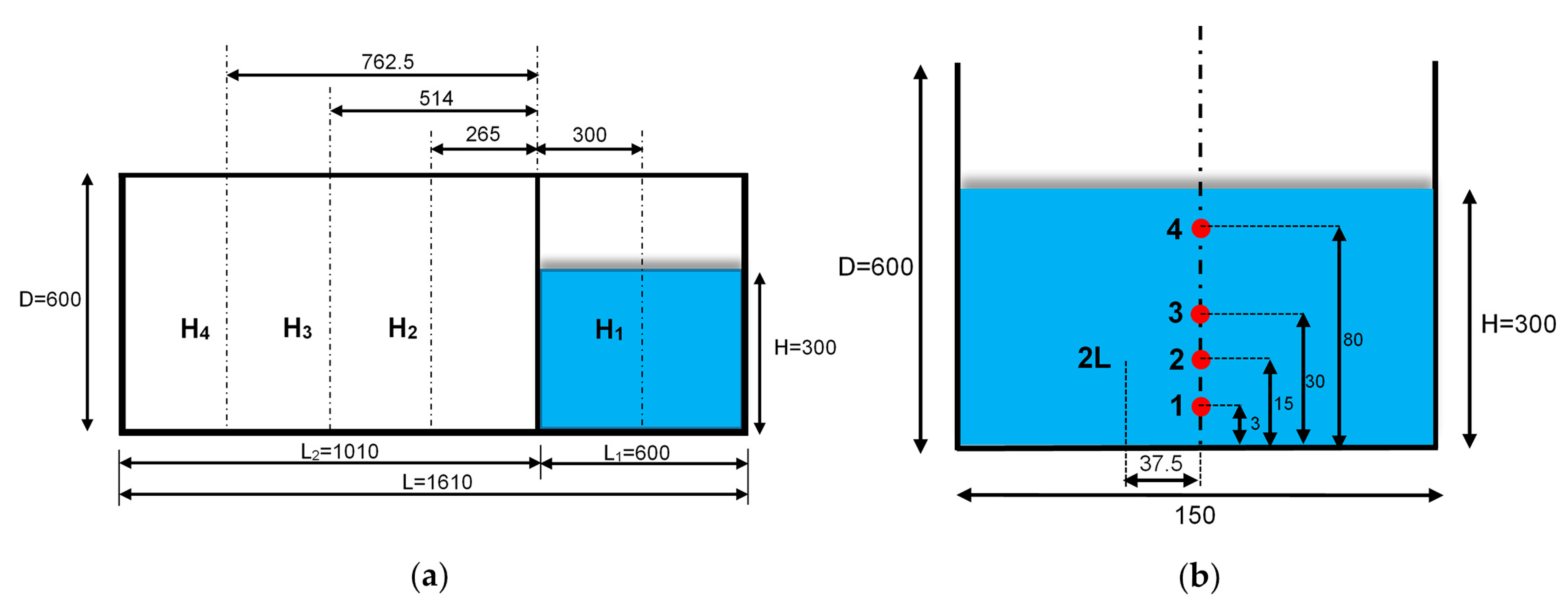
The model was applied to a large series of laboratory measures on a generally 2D dam-break flow [55] and to a H = 0.3 m water level in the reservoir in order to numerically reconstruct the free surface and the pressures acting on the downstream solid vertical wall. The experimental set-up, resembling the one by the authors of [56], consisted of a prismatic tank of 1610 × 600 × 150 mm, divided into two separate chambers by a removable gate placed at 600 mm from the lateral side (Figure 1). Before running each test, the bed and the downstream walls of the tank were kept completely dry.

The lateral, frontal, and top view of the complex free-surface profile evolution and the impact on the downstream wall were recorded by a digital camera, which also enabled the capture of the time history of the water level at several locations (i.e., H₁ = 300 mm in the reservoir, and H₂ = 265 mm, H₃ = 514 mm, and H₄ = 762.5 mm, all downstream of the gate). Given that the phenomenon under analysis was a gravity current flow with a horizontal bed, the Reynolds and the Weber numbers, based on both the distance between the gate and the wall and the predicted velocity of the wave front [60], were 3.8 × 10⁶ and 1.64 × 10⁵, respectively. Under these conditions of heavy turbulence in the boundary layer triggered by the advancing wave front, surface tension effects were negligible. The pressures were measured by five piezo-resistive sensors with an acquisition frequency of 20 kHz. Four were in the central line, and an additional one was placed halfway towards the back wall, to detect the presence of any 3D effects of the frontal impact wave. In detail, sensor 1 was positioned at 3 mm from the bottom of the tank, while sensors 2, 3, and 4 were, respectively, at 15 mm, 30 mm, and 80 mm above the bed; sensor 5 was installed at the same height as sensor 2.

4. Results and Discussion

The two advanced boundary treatment methods implemented in the SPHERA model [54], described respectively in Section 2.1 and Section 2.2, were validated with data from the experimental dam-break event carried out by the authors of [55] (see Section 3). In order to represent a sudden and complete dam-break, at the onset of the computation, water held under hydrostatic conditions is immediately released, rather than what occurs in the experimental setup, where the water is released gradually from a gate. This simplistic hypothesis is justified by the good agreement between the experiment and the SPH model in the representation of the time evolution of the primary wave, before the impact on the downstream wall. Moreover, the authors of [55] showed that the median value of the measured removal time is of the same order of magnitude as the theoretically predicted duration of the dam gate removal based on the freefall of the weight. In addition, the front side of the liquid block has not advanced beyond the position of the gate, which indicates that the gate rising speed is fast enough to disregard its effect on the liquid column.

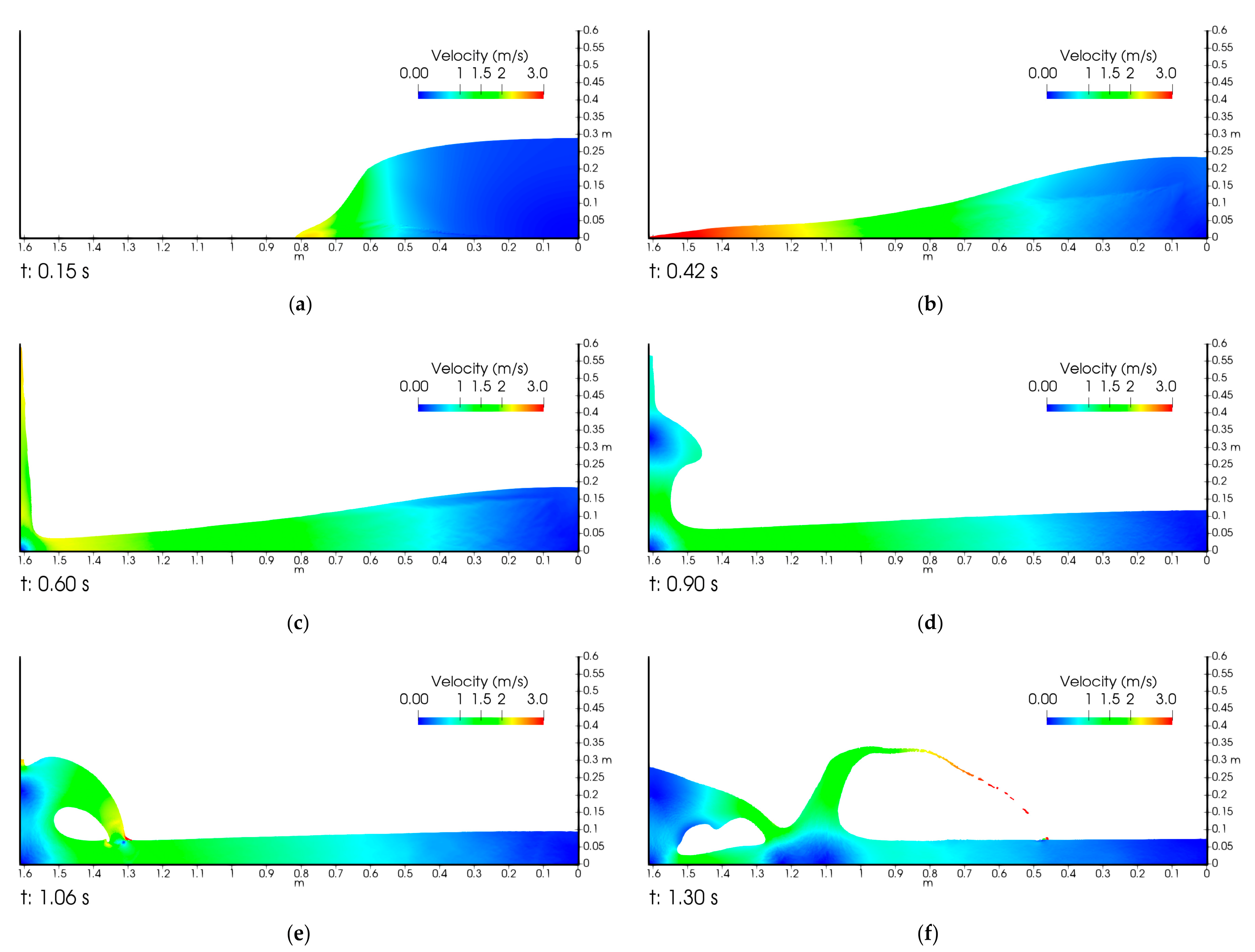
When the computation water held under hydrostatic conditions is released, a downstream wave advances along a dry bed towards the downstream vertical wall and, finally, strikes this wall (i.e., primary wave). Later, two different successive high vertical run-up jets, due to the inviscid model used (as highlighted also in [32,34]), are created and fall by gravity onto the underlying fluid. The second jet initially disintegrates into droplets that splash onto and are reabsorbed by the main volume of the fluid flow. It is notable that the proposed SPH model is not suitable for the treatment of the superficial cohesion of the fluid. The wave reflected by the downstream wall (i.e., the secondary wave) appears upstream as a unique plunging wave propagation combined with an air cushion. Several snapshots of the calculated free surface at several time instances are shown in Figure 2.

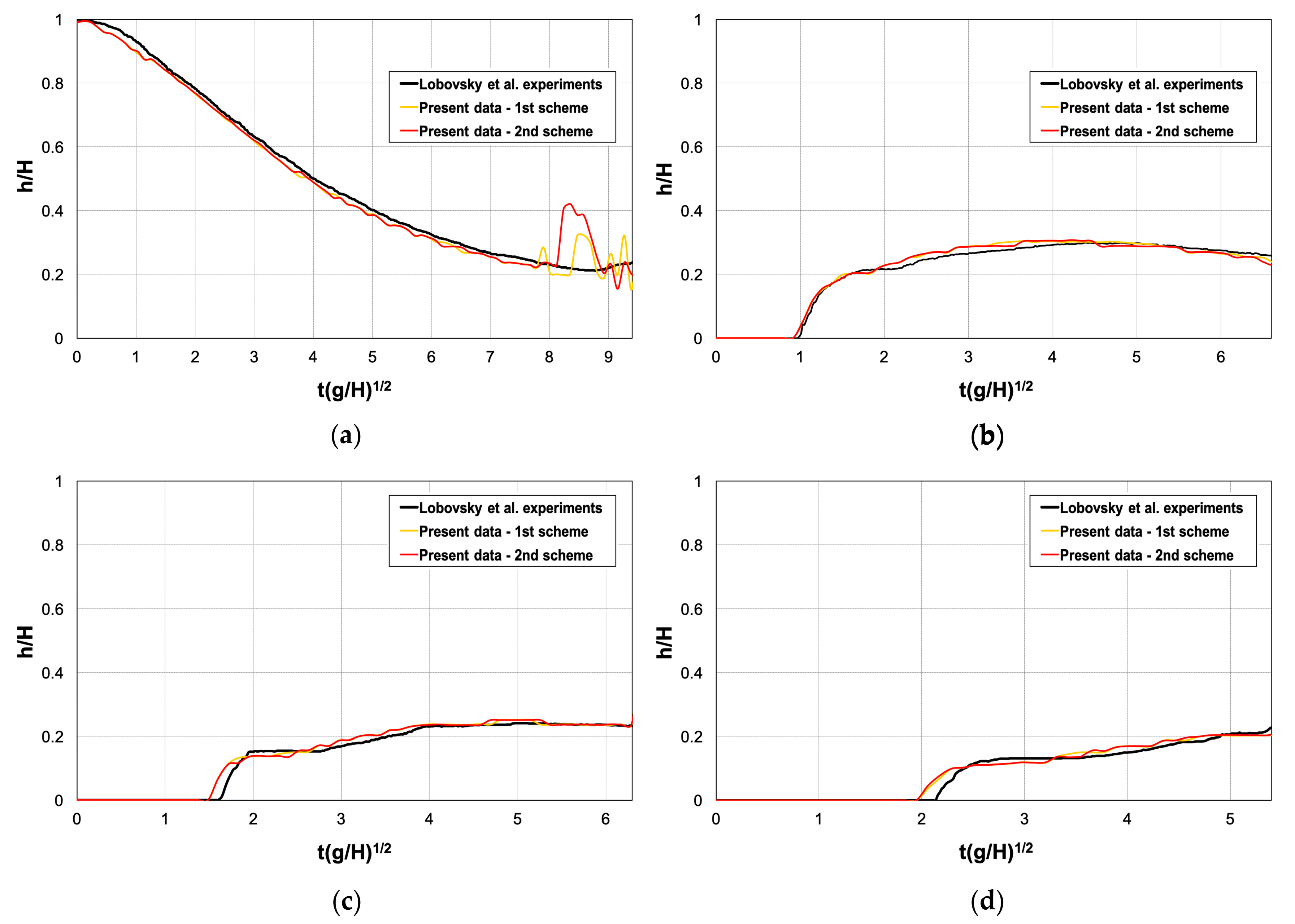
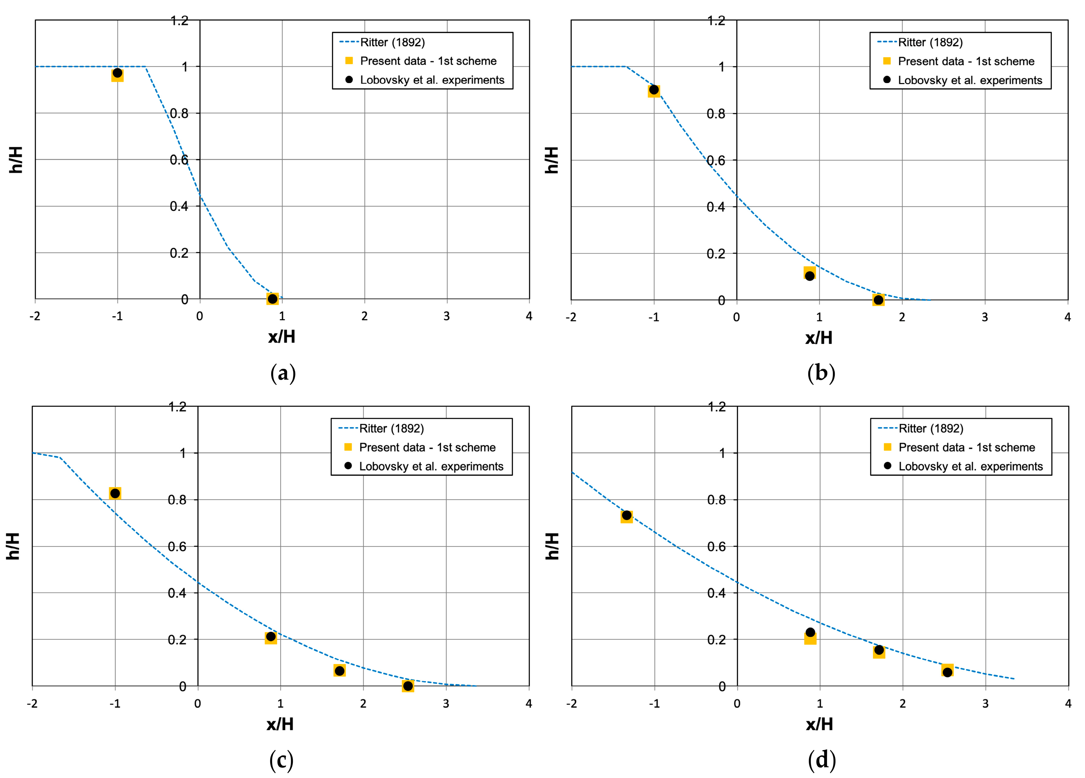
Figure 3 and Figure 4 report the experimental temporal evolution of water levels at locations H₁, H₂, H₃, and H₄ compared with those obtained using the first (green line) and the second (blue line) boundary treatment techniques. The numerical reconstruction of the free-surface profile from the gate release to the arrival of the secondary wave is pictured in Figure 3. The numerical and Lobovsky’s experimental [55] results at locations H₁, H₂, H₃, and H₄ have been compared with the longitudinal water surface profiles at several time instants from the gate release to the arrival of the secondary wave, obtained by the theoretical parabolic profile of Ritter [60]. The SPH simulation reproduces the theoretical solution well, as shown in Figure 4.

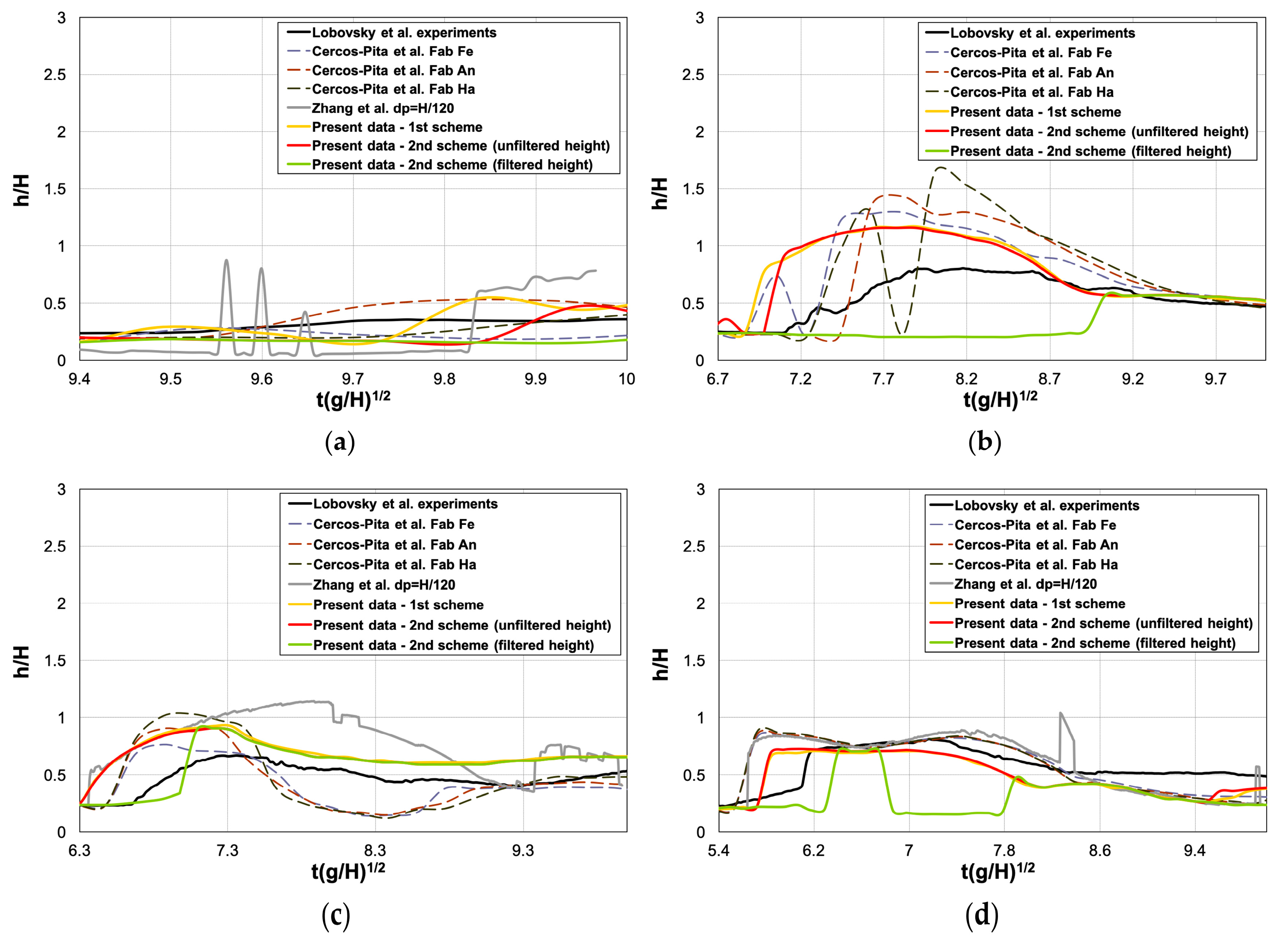
Figure 5 displays the evolution of water flow levels from the secondary wave’s arrival onward. In the latter case, the second scheme also includes the filtered height (red line) estimated along the same vertical, neglecting the breaking effects.

The distance of the wave front from the gate and the water levels are normalized by the initial height of the reservoir, H. The water levels are plotted against dimensionless time $t^{*}=\sqrt{g/H}$ (where t is the dimensional time recorded since the start of the gate’s movement, and g is the gravity acceleration magnitude). From Figure 3, both levels are generally in perfect agreement with the experimental trend for all sensors. Following the breaking of the reflected wave and the beginning of splashing, the signal acquired by the authors of [55] becomes noisy, due to both the flow fragmentation and the presence of complex vortex structures propagating along the channel and greatly affecting the water level at different locations. In fact, the authors of [55] stated: “The discrepancies in elevation of the secondary wave depend on complex flow structures that are created as the secondary wave propagates through the tank. These flow structures differ from case to case and significantly affect the water levels at specific locations. Thus, a question as to secondary flow repeatability emerges. This question remains open”. This poses a challenge not only with respect to the repeatability of the experimental signal and related uncertainty but also complicates its comparison with the proposed numerical reconstruction (Figure 4). In fact, both the simulations developed here and the curve by the authors of [34], with a particle resolution of dx = H/120 and the three curves from the authors of [32], obtained using different diffusive models, do not adequately represent water levels during the secondary wave.

More specifically, the filtered height curve of the second scheme is closer to the experimental data compared to the numerical results in the literature. The difference between the filtered and the unfiltered time series of the free surface height quantifies both the position of the multi-phase region (characterized by air intrusion) and the uncertainty in the definition of the free surface height. At the reflection of the primary dam-break wave, the filtering procedure on the free surface level provides differences comparable with the errors of the numerical code (with respect to measure). The filtering procedure locally reveals the presence of more than one liquid-gas interface along the vertical and possibly motivates either the use of a multi-phase model or the need for a clearer definition of the experimental procedure to detect the free surface.

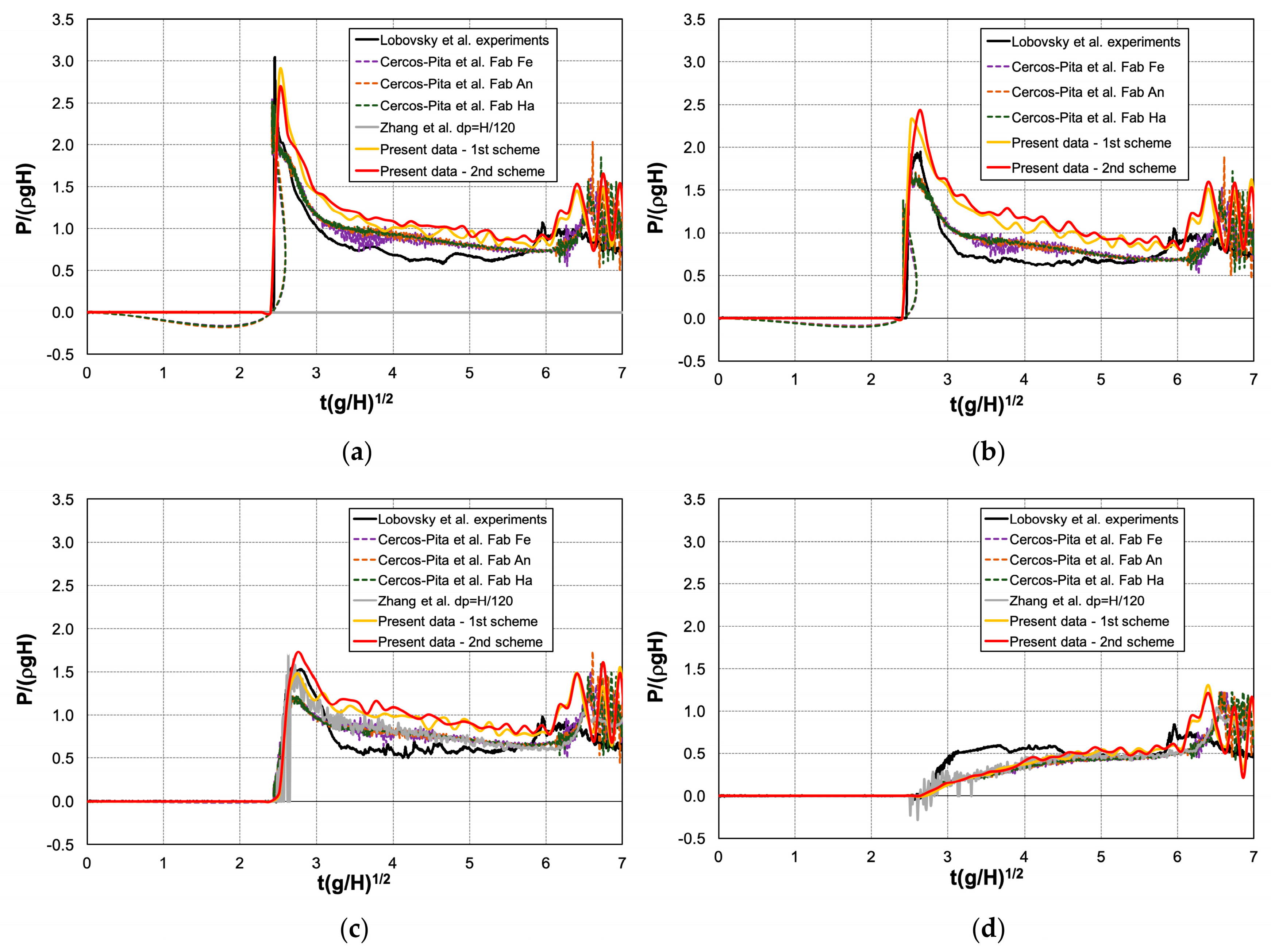
Finally, the numerical reconstruction of the impact wave pressures on the downstream vertical wall are presented in Figure 6. Here, the pressures are non-dimensionalized with regard to the hydrostatic pressure at the bottom of the reservoir and plotted versus t*. The trends of the pressures simulated with both the first and second scheme generally showed a close agreement with the experimental signals. The model developed here provides values slightly higher than those recorded by the authors of [55], especially for the probes P1, P2, and P4. In contrast, a lower pressure peak is produced for P3. Compared with previous numerical data, the present results show a smoother signal, a more pronounced overestimation of the pressure levels at 3 < t* <6, and a more correct assessment of the peak pressure.

5. Conclusions

A smoothed particle hydrodynamics method with two advanced boundary treatment techniques was proposed for modeling a free-surface flow with violent wave-breaking. Its efficiency and accuracy were validated by numerically simulating the dynamics of a two-dimensional dam-break event investigated by the authors of [55] in a laboratory prismatic tank with a removable gate.

The model generated an accurate representation of the wave’s free-surface profile and pressures on the downstream vertical wall seen in the experimental data. Both the advanced boundary techniques reproduced the water levels from the gate release to the arrival of the secondary wave with accuracy. Flow fragmentation and complex vortex structures propagating along the channel make a robust experimental reconstruction of the free surface profile of the secondary wave difficult, as widely discussed in previous studies. However, a comparison of the present work with numerical simulations in the literature highlights how the filtered height curve obtained from the second scheme, which neglects the breaking effects, is closer to the experimental data.

Finally, the temporal evolution of the pressures simulated with either techniques generally agrees well with the ones recorded by [55], providing slightly higher values, especially for the probes P1, P2, and P4, and a lower peak for P3. In the last time-step, the present data showed a more regular signal compared with the previous numerical results.

References

- Albano, R.; Mancusi, L.; Adamowski, J.; Cantisani, A.; Sole, A. A GIS Tool for Mapping Dam-Break Flood Hazards in Italy. ISPRS Int. J. Geo Inf. 2019, 8, 250. [Google Scholar] [CrossRef] [Green Version]
- Scarpino, S.; Albano, R.; Cantisani, A.; Mancusi, L.; Sole, A.; Milillo, G. Multitemporal SAR Data and 2D Hydrodynamic Model Flood Scenario Dynamics Assessment. ISPRS Int. J. Geo Inf. 2018, 7, 105. [Google Scholar] [CrossRef] [Green Version]
- Ferrari, A.; Fraccarollo, L.; Dumbser, M.; Toro, E.F.; Armanini, A. Three-dimensional flow evolution after a dam-break. J. Fluid Mech. 2010, 663, 456–477. [Google Scholar] [CrossRef]
- Liang, D. Evaluating shallow water assumptions in dam-break flows. Proc. Inst. Civ. Eng. Water Manag. 2010, 163, 227–237. [Google Scholar] [CrossRef]
- Manenti, S.; Wang, D.; Domínguez, J.M.; Li, S.; Amicarelli, A.; Albano, R. SPH Modeling of Water-Related Natural Hazards. Water 2019, 11, 1875. [Google Scholar] [CrossRef] [Green Version]
- Albano, R.; Manenti, S.; Domínguez, J.M.; Li, S.; Wang, D. Computational Methods and Applications to Simulate Water-Related Natural Hazards. Math. Probl. Eng. 2020, 4363095. [Google Scholar] [CrossRef]
- Liu, M.B.; Liu, G.R. Smoothed Particle Hydrodynamics (SPH): An Overview and Recent Developments. Arch. Comput. Methods Eng. 2010, 17, 25–76. [Google Scholar] [CrossRef] [Green Version]
- Amicarelli, A.; Kocak, B.; Sibilla, S.; Grabe, J. A 3D Smoothed Particle Hydrodynamics model for erosional dam-break floods. Int. J. Comput. Fluid D. 2017, 31, 413–434. [Google Scholar] [CrossRef]
- Vacondio, R.; Rogers, B.D.; Stansby, P.; Mignosa, P. SPH Modeling of Shallow Flow with Open Boundaries for Practical Flood Simulation. J. Hydraul. Eng. 2012, 138, 530–541. [Google Scholar] [CrossRef]
- Amicarelli, A.; Leuzzi, G.; Monti, P.; Alessandrini, S.; Ferrero, E. A stochastic Lagrangian micromixing model for the dispersion of reactive scalars in turbulent flows: Role of concentration fluctuations and improvements to the conserved scalar theory under non-homogeneous conditions. Environ. Fluid Mech. 2017, 17, 715–753. [Google Scholar] [CrossRef]
- He, J.; Tofighi, N.; Yildiz, M.; Lei, J.; Suleman, A. A Coupled WC-TL SPH Method for Simulation of Hydroelastic Problems. Int. J. Comput. Fluid D. 2017, 31, 174–187. [Google Scholar] [CrossRef]
- Colagrossi, A.; Souto-Iglesias, A.; Antuono, M.; Marrone, S. Smoothed-Particle-Hydrodynamics Modeling of Dissipation Mechanisms in Gravity Waves. Phys. Rev. E Stat. Nonlin. Soft Matter Phys. 2013, 87, 023302. [Google Scholar] [CrossRef] [PubMed]
- Espa, P.; Sibilla, S.; Gallati, M. SPH Simulations of a Vertical 2-D Liquid Jet Introduced from the Bottom of a Free-Surface Rectangular Tank. Adv. Appl. Fluid Mech. 2008, 3, 105–140. [Google Scholar]
- Price, D.J. Smoothed Particle Hydrodynamics and Magneto hydrodynamics. J. Comput. Phys. 2012, 231, 759–794. [Google Scholar] [CrossRef] [Green Version]
- Amicarelli, A.; Albano, R.; Mirauda, D.; Agate, G.; Sole, A.; Guandalini, R. A Smoothed Particle Hydrodynamics Model for 3D Solid Body Transport in Free Surface Flows. Comput. Fluids 2015, 116, 205–228. [Google Scholar] [CrossRef]
- Manenti, S.; Sibilla, S.; Gallati, M.; Agate, G.; Guandalini, R. SPH Simulation of Sediment Flushing Induced by a Rapid Water Flow. J. Hydraul. Eng. 2012, 138, 227–311. [Google Scholar] [CrossRef]
- Abdelrazek, A.M.; Kimura, I.; Shimizu, Y. Simulation of Three-Dimensional Rapid Free-Surface Granular Flow Past Different Types of Obstructions Using the SPH Method. J. Glaciol. 2016, 62, 335–347. [Google Scholar] [CrossRef] [Green Version]
- Danis, M.E.; Orhan, M.; Ecder, A. ISPH Modelling of Transient Natural Convection. Int. J. Comput. Fluid D. 2013, 27, 15–31. [Google Scholar] [CrossRef]
- Colagrossi, A.; Landrini, M. Numerical Simulation of Interfacial Flows by Smoothed Particle Hydrodynamics. J. Comput. Phys. 2003, 191, 448–475. [Google Scholar] [CrossRef]
- Antoci, C.; Gallati, M.; Sibilla, S. Numerical Simulation of Fluid-Structure Interaction by SPH. Comput. Struct. 2007, 85, 879–890. [Google Scholar] [CrossRef]
- Crespo, A.J.; Gómez-Gesteira, M.; Dalrymple, R.A. Modeling Dam-break Behavior over a Wet Bed by a SPH Technique. J. Waterw. Port. Coast. Ocean. Eng. 2008, 134, 313–320. [Google Scholar] [CrossRef]
- Khayyer, A.; Gotoh, H. On Particle-Based Simulation of a Dam-break over a Wet bed. J. Hydraul. Res. 2010, 48, 238–249. [Google Scholar] [CrossRef]
- Marrone, S.; Antuono, M.; Colagrossi, A.; Colicchio, G.; Le Touzé, D.; Graziani, G. ?-SPH Model for Simulating Violent Impact Flows. Comput. Methods Appl. Mech. Eng. 2011, 200, 1526–1542. [Google Scholar] [CrossRef]
- Chang, T.J.; Kao, H.M.; Chang, K.H.; Hsu, M.H. Numerical simulation of shallow-water dam-break flows in open channels using smoothed particle hydrodynamics. J. Hydrol. 2011, 408, 78–90. [Google Scholar] [CrossRef]
- Kao, H.M.; Chang, T.J. Numerical modeling of dambreak-induced flood and inundation using smoothed particle hydrodynamics. J. Hydrol. 2012, 448–449, 232–244. [Google Scholar] [CrossRef]
- Pu, J.H.; Shao, S.; Huang, Y.; Hussain, K. Evaluations of SWEs and SPH Numerical Modelling Techniques for Dam-break Flows. Eng. Appl. Comput. Fluid Mech. 2013, 7, 544–563. [Google Scholar]
- Wu, J.; Zhang, H.; Dalrymple, R.A.; Hérault, A. Numerical modeling of Dam-Break Flood in City Layouts Including Underground Spaces Using GPU-Based SPH Method. J. Hydrodynam. 2013, 25, 818–828. [Google Scholar] [CrossRef]
- St-Germain, P.; Nistor, I.; Townsend, R.; Shibayama, T. Smoothed-Particle Hydrodynamics Numerical Modeling of Structures Impacted by Tsunami Bores. J. Waterway Port. Coastal Ocean. Eng. 2014, 140, 66–81. [Google Scholar] [CrossRef]
- Nishiura, D.; Wüthrich, D.; Furuichi, M.; Nomura, S.; Pfister, M.; De Cesare, G. Numerical Approach in the Study of Tsunami-like Waves and Comparison with Experimental Data. In Proceedings of the Twenty-ninth International Ocean and Polar Engineering Conference, Honolulu, HI, USA, 16–21 June 2019; pp. 3166–3173. [Google Scholar]
- Wüthrich, D.; Nishiura, D.; Furuichi, M.; Nomura, S.; Pfister, M.; De Cesare, G. Experimental and numerical study on wave-impact on buildings. In Proceedings of the 38th IAHR World Congress, Panama City, Panama, 1–6 September 2019; pp. 6047–6056. [Google Scholar] [CrossRef]
- Jian, W.; Liang, D.; Shao, S.; Chen, R.; Liu, X. SPH study of the evolution of water-water interfaces in dam-break flows. Nat. Hazards 2015, 78, 531–553. [Google Scholar] [CrossRef] [Green Version]
- Cercos-Pita, J.L.; Dalrymple, R.A.; Herault, A. Diffusive terms for the conservation of mass equation in SPH. Appl. Math. Model. 2016, 40, 8722–8736. [Google Scholar] [CrossRef]
- Gu, S.; Zheng, X.; Ren, L.; Xie, H.; Huang, Y.; Wei, J.; Shao, S. SWE-SPHysics Simulation of Dam-break Flows at South-Gate Gorges Reservoir. Water 2017, 9, 387. [Google Scholar] [CrossRef] [Green Version]
- Zhang, C.; Hu, X.Y.; Adams, N.A. A weakly compressible SPH method based on a low-dissipation Riemann solver. J. Comput. Phys. 2017, 335, 605–620. [Google Scholar] [CrossRef]
- Albano, R.; Sole, A.; Mirauda, D.; Adamowski, J. Modelling large floating bodies in urban area flash-floods via a Smoothed Particle Hydrodynamics model. J. Hydrol. 2016, 541, 344–358. [Google Scholar] [CrossRef]
- Amicarelli, A.; Agate, G.; Guandalini, R. A 3D Fully Lagrangian Smoothed Particle Hydrodynamics model with both volume and surface discrete elements. Int. J. Numer. Meth. Eng. 2013, 95, 419–450. [Google Scholar] [CrossRef]
- Monaghan, J.J.; Koss, A. Solitary waves on a Cretan beach. J. Waterw. Port. Coast. Ocean. Eng. 2002, 125, 145–155. [Google Scholar] [CrossRef]
- Monaghan, J.J. Simulating free surface flows with SPH. J. Comput. Phys. 1994, 110, 399–406. [Google Scholar] [CrossRef]
- Lobovský, L.; Groenenboomb, P.H.L. Smoothed particle hydrodynamics modelling in continuum mechanics: Fluid-structure interaction. ACM 2009, 3, 101–110. [Google Scholar]
- Yildiz, M.; Rook, R.A.; Suleman, A. SPH with the boundary tangent method. Int. J. Numer. Meth. Eng. 2009, 77, 1416–1438. [Google Scholar] [CrossRef] [Green Version]
- Fourtakas, G.; Vacondio, R.; Rogers, B.D. On the approximate zeroth and first-order consistency in the presence of 2-D irregular boundaries in SPH obtained by the virtual boundary particle methods. Int. J. Num. Meth. Fl. 2015, 78, 475–501. [Google Scholar] [CrossRef]
- Adami, S.; Hu, X.Y.; Adams, N.A. A generalized wall boundary condition for smoothed particle hydrodynamics. J. Comput. Phys. 2012, 231, 7057–7075. [Google Scholar] [CrossRef]
- Crespo, A.J.C.; Gómez-Gesteira, M.; Dalrymple, R.A. Boundary conditions generated by dynamic particles in SPH methods. CMC Comput. Mater. Contin. 2007, 5, 173–184. [Google Scholar]
- Gómez-Gesteira, M.; Rogers, B.D.; Crespo, A.J.C.; Dalrymple, R.A.; Narayanaswamy, M.; Dominguez, J.M. SPHysics-development of a free surface fluid solver-part 1: Theory and formulations. Comput. Geosci. 2012, 48, 289–299. [Google Scholar] [CrossRef]
- Fraga Filho, C.A.D.; Chacaltana, J.T.A. Boundary treatment techniques in smoothed particle hydrodynamics: Implementations in fluid and thermal sciences and results analysis. In Proceedings of the XXXVII Iberian Latin American Congress on Computational Methods in Engineering (CILAMCE 2016), Brasília, DF, Brazil, 6–9 November 2016. [Google Scholar]
- House, D.H.; Keyser, J.C. Foundations of Physically Based Modeling & Animation, 1st ed.; CRC Press—Taylor & Francis Group: Boca Raton, FL, USA, 2017. [Google Scholar]
- Fraga Filho, C.A.D. An algorithmic implementation of physical reflective boundary conditions in particle methods: Collision detection and response. Phys. Fluids 2017, 29, 113602. [Google Scholar] [CrossRef]
- Kulasegaram, S.; Bonet, J.; Lewis, R.W.; Profit, M. A variational formulation based contact algorithm for rigid boundaries in two-dimensional SPH applications. Comput. Mech. 2004, 33, 316–325. [Google Scholar] [CrossRef]
- Ferrand, M.; Laurence, D.R.; Rogers, B.D.; Violeau, D.; Kassiotis, C. Unified semi-analytical wall boundary conditions for inviscid, laminar or turbulent flows in the meshless SPH method. Int. J. Num. Meth. Fl. 2013, 71, 446–472. [Google Scholar] [CrossRef] [Green Version]
- Leroy, A.; Violeau, D.; Ferrand, M.; Kassiotis, C. Unified semi-analytical wall boundary conditions applied to 2-D incompressible SPH. J. Comput. Phys. 2014, 261, 106–129. [Google Scholar] [CrossRef] [Green Version]
- Mayrhofer, A.; Ferrand, M.; Kassiotis, C.; Violeau, D.; Morel, F. Unified semi-analytical wall boundary conditions in SPH: Analytical extension to 3-D. Numer. Algor. 2015, 68, 15–34. [Google Scholar] [CrossRef]
- Macià, F.; Gonzales, L.M.; Cercos-Pita, J.L.; Souto-Iglesias, A.A. Boundary Integral SPH Formulation—Consistency and Applications to ISPH and WCSPH. Prog. Theor. Phys. 2012, 128, 439–462. [Google Scholar] [CrossRef] [Green Version]
- Chiron, L.; De Leffe, M.; Oger, G.; Le Touzé, D. Fast and accurate SPH modelling of 3D complex wall boundaries in viscous and non viscous flows. Comput. Phys. Commun. 2019, 234, 93–111. [Google Scholar] [CrossRef]
- Amicarelli, A.; Manenti, S.; Albano, R.; Agate, G.; Paggi, M.; Longoni, L.; Mirauda, D.; Ziane, L.; Viccione, G.; Todeschini, S.; et al. SPHERA v.9.0.0: A Computational Fluid Dynamics research code, based on the Smoothed Particle Hydrodynamics mesh-less method. Comput. Phys. Commun. 2020, 250, 107157. [Google Scholar] [CrossRef]
- Lobovský, L.; Botia-Vera, E.; Castellana, F.; Mas-Soler, J.; Souto-Iglesias, A. Experimental investigation of dynamic pressure loads during dam-break. J. Fluids Struct. 2014, 48, 407–434. [Google Scholar] [CrossRef] [Green Version]
- Lee, T.; Zhou, Z.; Cao, Y. Numerical simulations of hydraulic jumps in water sloshing and water impacting. J. Fluids Eng. 2002, 124, 215–226. [Google Scholar] [CrossRef]
- Di Monaco, A.; Manenti, S.; Gallati, M.; Sibilla, S.; Agate, G.; Guandalini, R. SPH modeling of solid boundaries through a semi-analytic approach. Eng. Appl. Comput. Fluid Mech. 2011, 5, 1–15. [Google Scholar] [CrossRef]
- Vila, J.P. On particle weighted methods and Smooth Particle Hydrodynamics. Math. Models Methods Appl. Sci. 1999, 9, 161–209. [Google Scholar] [CrossRef]
- Monaghan, J.J. Smoothed particle hydrodynamics. Rep. Prog. Phys. 2005, 68, 1703–1759. [Google Scholar] [CrossRef]
- Ritter, A. Die Fortpflanzung de Wasserwellen. Z. Ver. Deutscher Ingenieure Ger. 1892, 36, 947–954. [Google Scholar]
Figure 1.
Experimental set-up: (a) water level measuring position on the left (lateral view); (b) pressure sensor locations on the right (frontal view). Dimensions are in millimeters.
Figure 2.
Two-dimensional dam-break phenomena: field snapshots of the absolute value of velocity at several time instants: (a) t = 0.15 s; (b) t = 0.42 s; (c) t = 0.60 s; (d) t = 0.90 s; (e) t = 1.06 s; and (f) t = 1.30 s.
Figure 3.
Comparison between the experimental and numerical water level elevations at locations: (a) H1; (b) H2; (c) H3; and (d) H4 over time, until the arrival of the secondary wave.
Figure 4.
Comparison between the experimental and the numerical water level elevations at locations: (a) H1; (b) H2; (c) H3; and (d) H4 with the Ritter theoretical solution at t = 0.1 s, t = 0.2 s, t = 0.3 s, and t = 0.4 s, until the arrival of the secondary wave.
Figure 5.
Water surface elevation comparison between the numerical results and the experimental data from the secondary wave arrival: (a) H1; (b) H2; (c) H3; and (d) H4.
Figure 6.
Temporal evolution of pressure simulated at: (a) P1; (b) P2; (c) P3; and (d) P4 located on the downstream vertical wall of the channel. Comparison between experimental and numerical data in the literature.
© 2020 by the authors. Licensee MDPI, Basel, Switzerland. This article is an open access article distributed under the terms and conditions of the Creative Commons Attribution (CC BY) license (http://creativecommons.org/licenses/by/4.0/).
Share and Cite
MDPI and ACS Style
Mirauda, D.; Albano, R.; Sole, A.; Adamowski, J. Smoothed Particle Hydrodynamics Modeling with Advanced Boundary Conditions for Two-Dimensional Dam-Break Floods. Water 2020, 12, 1142. https://doi.org/10.3390/w12041142
AMA Style
Mirauda D, Albano R, Sole A, Adamowski J. Smoothed Particle Hydrodynamics Modeling with Advanced Boundary Conditions for Two-Dimensional Dam-Break Floods. Water. 2020; 12(4):1142. https://doi.org/10.3390/w12041142
Chicago/Turabian StyleMirauda, Domenica, Raffaele Albano, Aurelia Sole, and Jan Adamowski. 2020. "Smoothed Particle Hydrodynamics Modeling with Advanced Boundary Conditions for Two-Dimensional Dam-Break Floods" Water 12, no. 4: 1142. https://doi.org/10.3390/w12041142
Note that from the first issue of 2016, this journal uses article numbers instead of page numbers. See further details here.