Total Maximum Allocated Load of Chemical Oxygen Demand Near Qinhuangdao in Bohai Sea: Model and Field Observations
by
Zhichao Dong
1, 
Cuiping Kuang
1,*, 
Jie Gu
2,
Qingping Zou
3,*,
Jiabo Zhang
4,
Huixin Liu
4 and
Lei Zhu
4 1
College of Civil Engineering, Tongji University, Shanghai 200092, China
2
College of Marine Ecology and Environment, Shanghai Ocean University, Shanghai 201306, China
3
The Lyell Centre for Earth and Marine Science and Technology, Institute for Infrastructure and Environment, Heriot-Watt University, Edinburgh EH14 4AS, UK
4
The Eighth Geological Brigade, Hebei Geological Prospecting Bureau, Qinhuangdao 066001, China
*
Authors to whom correspondence should be addressed.
Water 2020, 12(4), 1141; https://doi.org/10.3390/w12041141
Submission received: 17 March 2020
/
Revised: 11 April 2020
/
Accepted: 14 April 2020
/
Published: 16 April 2020
(This article belongs to the Section Water Quality and Contamination)
Abstract
:Total maximum allocated load (TMAL) is the maximum sum total of all the pollutant loading a water body can carry without surpassing the water quality criterion, which is dependent on hydrodynamics and water quality conditions. A coupled hydrodynamic and water quality model combined with field observation was used to study pollutant transport and TMAL for water environment management in Qinhuangdao (QHD) sea in the Bohai Sea in northeastern China for the first time. Temporal and spatial variations of the chemical oxygen demand (COD) concentration were investigated based on MIKE suite (Danish Hydraulic Institute, Hørsholm, Denmark). A systematic optimization approach of adjusting the upstream pollutant emission load was used to calculate TMAL derived from the predicted COD concentration. The pollutant emission load, TMAL, and pollutant reduction of Luanhe River were the largest due to the massive runoff, which was identified as the most influential driving factor for water environmental capacity and total carrying capacity of COD. The correlation analysis and Spearman coefficient indicate strong links between TMAL and forcing factors such as runoff, kinetic energy, and pollutant emission load. A comparison of total carrying capacity in 2011 and 2013 confirms that the upstream pollutant control scheme is an effective strategy to improve water quality along the river and coast. Although, the present model results suggest that a monitoring system could provide more efficient total capacity control. The outcome of this study establishes the theoretical foundation for coastal water environment management strategy in this region and worldwide.
1. Introduction
With growing industrialization and urbanization, effluent discharge and human activities impose increasing pressure on coastal ecosystems and natural resources, especially in densely populated coastal zones [1]. Coastal water is contaminated by discharge of land-based pollutant and marine aquaculture, which causes increasing water pollution for residents as well as risk of eutrophication. Red tide and harmful algal bloom due to eutrophication are common phenomena in coastal regions in recent years [2,3,4]. Stricter limits for pollutant emissions and effective coastal management are vital to prevent water pollution and improve the coastal environment [5,6].
In fact, the upper limit of pollutant discharging into a coastal area has been identified as the environmental carrying capacity by GESAMP (Joint Group of Experts on the Scientific Aspects of Marine Environmental Protection) [7]. The environmental capacity is a quantitative description of pollution accommodation capacity under the premise of no harm on the ecological system [8], which ensures sustainable coastal zone development [9]. The quantity of pollutant transported to the open sea was estimated by the water exchange rate and observations of water quality and hydrodynamics, and the transport quantity was determined as the environmental capacity in the 1980s [10]; however, this method has suffered from discontinuity of data and human factors. A numerical model was instead used to supplement data and simulate water quality conditions; through calibration and validation combined with observation data, most of the physical and biogeochemical processes in the coastal area were obtained [11,12,13]. Hence, numerical simulation has become a popular technique to assess environmental capacity based on optimization of the water quality simulation process [14,15,16].
Focusing on water environmental capacity, management of pollutant sources mainly relies on water quality as an indicator [17]. In the past decades, many water management techniques were examined extensively in many countries [18,19,20]. The Total Pollutant Load Control System (TPLCS) was established as part of national regulations and laws in Japan and has been applied to Tokyo Bay, Ise Bay, and Seto Island Sea since the 1970s [21]. The TPLCS focuses on limiting pollutant emission and preventing pollution discharge without certificates. Pollutants are effectively controlled by the TPLCS; in fact, Japan has changed since the 1960s and is no longer a larger polluter but instead is a clean developed country [22,23]. In America, the total maximum daily load (TMDL) has been used as a key measure to ensure surface water quality is up to health standards. TMDL has developed and improved for more than 20 years and forms a set of integrated total pollutant control strategies and technique systems, which are not only used in coastal areas but also in lakes and watersheds [24,25]. Since the total pollutant control and comprehensive treatment measures were used in European countries, the water qualities of the Rhine and Baltic Sea have improved markedly due to efficient management of industrial and sanitary wastewater emission [26,27]. The Coastal Pollution Total Load Control Management (CPTLCM) has been implemented to improve the coastal water environment in China. The total maximum allocated load (TMAL) has been used to assess the maximum pollutant emission under the water quality criterion described in the “National Marine Water Quality Criteria” (GB 3097-1997) [28,29].
Eutrophication is the major cause of ecological disasters such as algae bloom [30]. Chemical oxygen demand (COD) is the key contributing factor to eutrophication by providing a carbon source for phytoplankton and algae growth [31]. However, COD transport in a coastal area is complex due to combined action of runoff and tide [11]. The eutrophication in Qinhuangdao (QHD) in the Bohai Sea has increased due to increased discharge of domestic, industrial, and agricultural wastewater, therefore harmful algae occur more frequently [32]. Thus, COD was chosen as an indicator for TMAL in this study.
QHD was voted as one of the top ten ecological cities in China and the most well-recognized coastal resort. As the destination city of recreational tourism, QHD is required to maintain a high water quality. To achieve the water quality criteria, the QHD coastal area has adopted integrated systematic management and development strategies covering all seagoing rivers and coastal water. The TMAL is mainly determined by water quality field data collected under multiple forcing conditions, including hydrodynamics, source discharge, and human activities [33,34]. In this study, a coupled hydrodynamic and water quality model combined with field observations was used to investigate the spatial and temporal variations of water quality in QHD for the first time, from which environmental capacity and total capacity control were derived through an optimization approach of adjusting the upstream pollutant emission. Seasonal variations of TMAL, emission load, and pollutants were analyzed and linked with hydrodynamic variables and correlations between TMAL, runoff, kinetic energy, and emission load were obtained. The comparison of water environmental capacity and total capacity control of pollutants over the past years indicates that the environment management regulations and strategies efficiently improved QHD coastal water quality. The objective of the present study is to better understand the driving mechanisms of water environmental capacity in the coastal area of QHD. The outcome of this study should provide guidelines for robust coastal water environment management strategies in other coastal regions around the globe.
2. Field Site and Model Setup
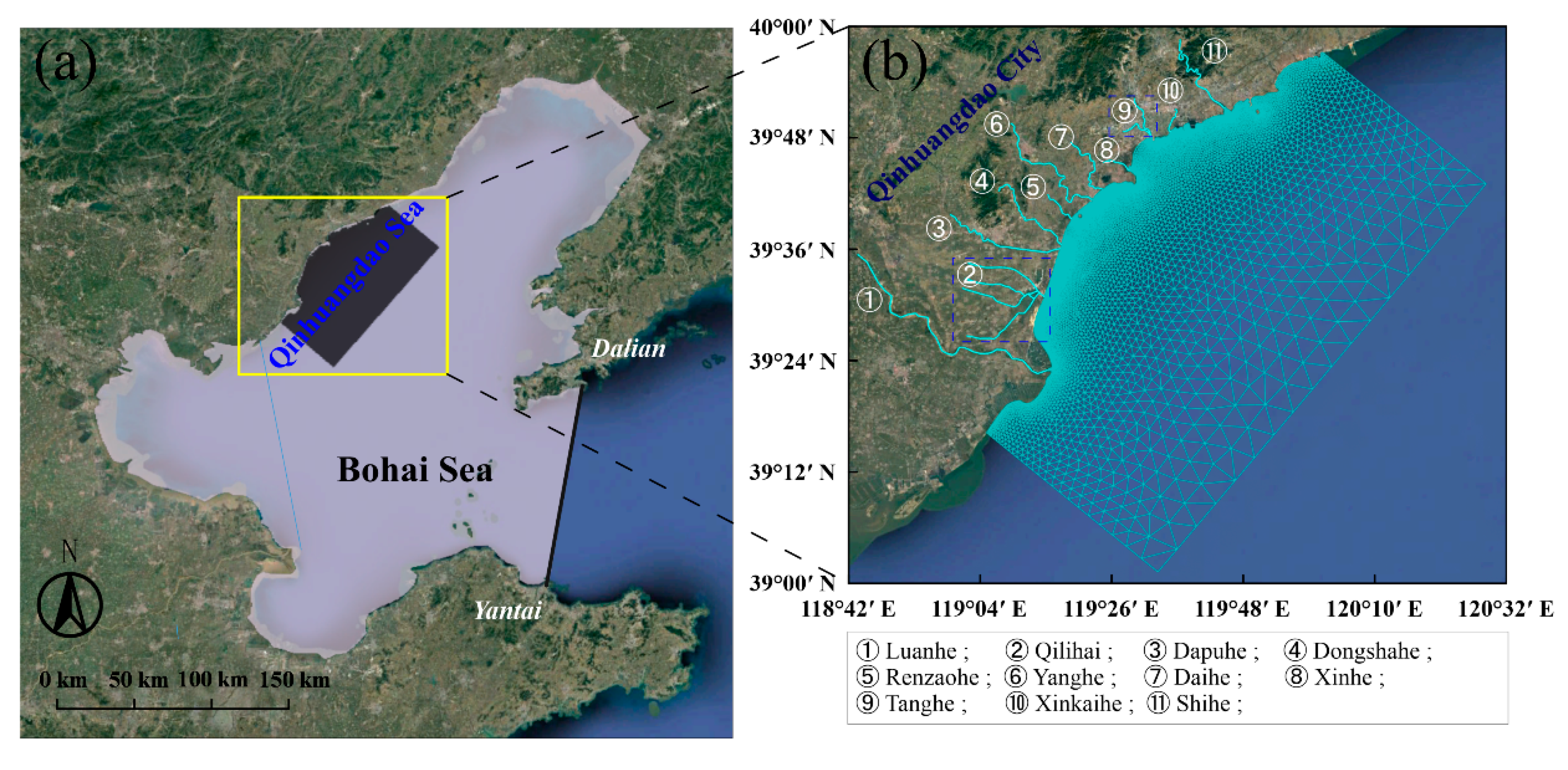
QHD is located in the northeastern Hebei Province in China and adjacent to the Bohai Sea (39°24′~40°37′ N, 118°33′~119°51′ E). A large amount of recreational bathing beaches are distributed along the 163 km coastline of QHD, as shown in Figure 1. QHD is within the middle latitude zone with a humid and semi-humid continental monsoon climate of a warm temperate zone. QHD has an annual sunshine duration of 2700~2850 h, temperature of 8.8~11.3 °C, precipitation of 650~750 mm, and average evaporation of 1468.7 mm. Since the average temperature of QHD in winter is −3.7 °C, the rivers in QHD are frozen for about 108 days from 21 November to 31 March [35].
QHD has a drainage basin over 30 km2 and an annual average runoff volume of 12.6 × 10⁸ m3. The interannual variation of runoff ranges from 2.5 × 10⁸ to 41.8 × 10⁸ m3. River flow in QHD area comes from a northwest to southeast direction before discharging into the Bohai Sea. Qilihai Lagoon collects water from four rivers and the Tanghe estuary from two rivers, which are approximated as one river. Thus there are 11 seagoing rivers including Luanhe River (LH), Qilihai Lagoon (QLH), Dapuhe River (DPH), Dongshahe River (DSH), Renzaohe River (RZH), Yanghe River (YH), Daihe River (DH), Xinhe River (XH), Tanghe River (TH), Xinkaihe River (XKH), and Shihe River (SH) from south to north, as numbered and indicated in Figure 1b. The rainfall mainly occurs during summer and autumn, and rarely during spring and winter, which causes significant seasonal variation of runoff. The annual mean runoff in 2013 ranged from 0.25 m3/s to 39.74 m3/s.
According to the marine function zoning regulation in Hebei Province (2011–2020), QHD is within the scenic tourism and recreational entertainment zone and boasts one of the best bathing beaches in China. In addition to tourism, mariculture is also important to the local economy. It follows that QHD has to meet the requirements of the criterion of second category water quality [36]. The COD has to be less than or equal to 3.0 mg/L based on the criterion of second category water quality according to the “National Marine Water Quality Criteria” (GB3097-1997) [37].
3. Methodology
3.1. Hydrodynamic and Water Quality Model
TMAL was calculated based on hydrodynamic and water quality models. Field observations tended to be point measurements, whereas numerical simulation captured both spatial and temporal variations of hydrodynamics and contamination. MIKE 21 FM (flow model) is a two-dimensional modeling system in MIKE suite (Release 2014), which was applied in this study to simulate the hydrodynamic and pollutant transport. In MIKE 21 FM coupled with the hydrodynamic model, the water quality model was driven by tide and runoff. Using Boussinesq approximation, hydrostatic pressure, and shallow water conditions, the Reynolds averaged Navier–Stokes equations were reduced to generalized shallow water equations using the controlling volume method. The governing equations of the numerical model are demonstrated in the Appendix A [38].
The unstructured nested grid from the Bohai Sea to QHD was constructed based on World Geodetic System 1984 (Figure 1b). The larger mesh of the Bohai Sea took the line connecting the tide stations of Dalian and Yantai as the offshore boundary, whose tidal level data were from the National Marine Data and Information Service of China [39]. Then the larger mesh domain provided a tidal level boundary for smaller mesh domain of the QHD sea. The mesh of QHD has 9442 nodes and 17,973 elements with WE span of 110 km and NS span of 120 km. The mesh size is 7 km in the open sea and 15 m near the coastline. The higher resolution near the coastline is necessary to resolve the complex coastal bathymetry and shoreline.
The boundary conditions at 11 river mouths were set by monthly average runoff and COD discharge in 2013. The flood season is from June to September and the largest runoff for each river occurs in July or August. December to March are the dry months with less runoff. LH is the largest river in QHD, with runoff much larger than other rivers. The mean discharge was over 1.72 × 10⁹ t from July to September with a peak value of 4.28 × 10⁹ t in August. Bottom stress was determined by a quadratic friction law with a bottom roughness from 0.01 to 0.015 s/m1/3 through water depth and sediment diameter.
For the water quality model, non-conservative matter such as COD was not only influenced by flow convection and diffusion, but also by degradation processes such as microbial assimilation and metabolism. The initial COD concentration was set as the historical average value of 1.3 mg/L, and the decay rate for degradation was 0.03/d through model calibration [11]. The horizontal dispersion was determined by the eddy viscosity formulation dependent on the Prandtl number which was set as 1 by calibration in this study [40].
3.2. Field Observations
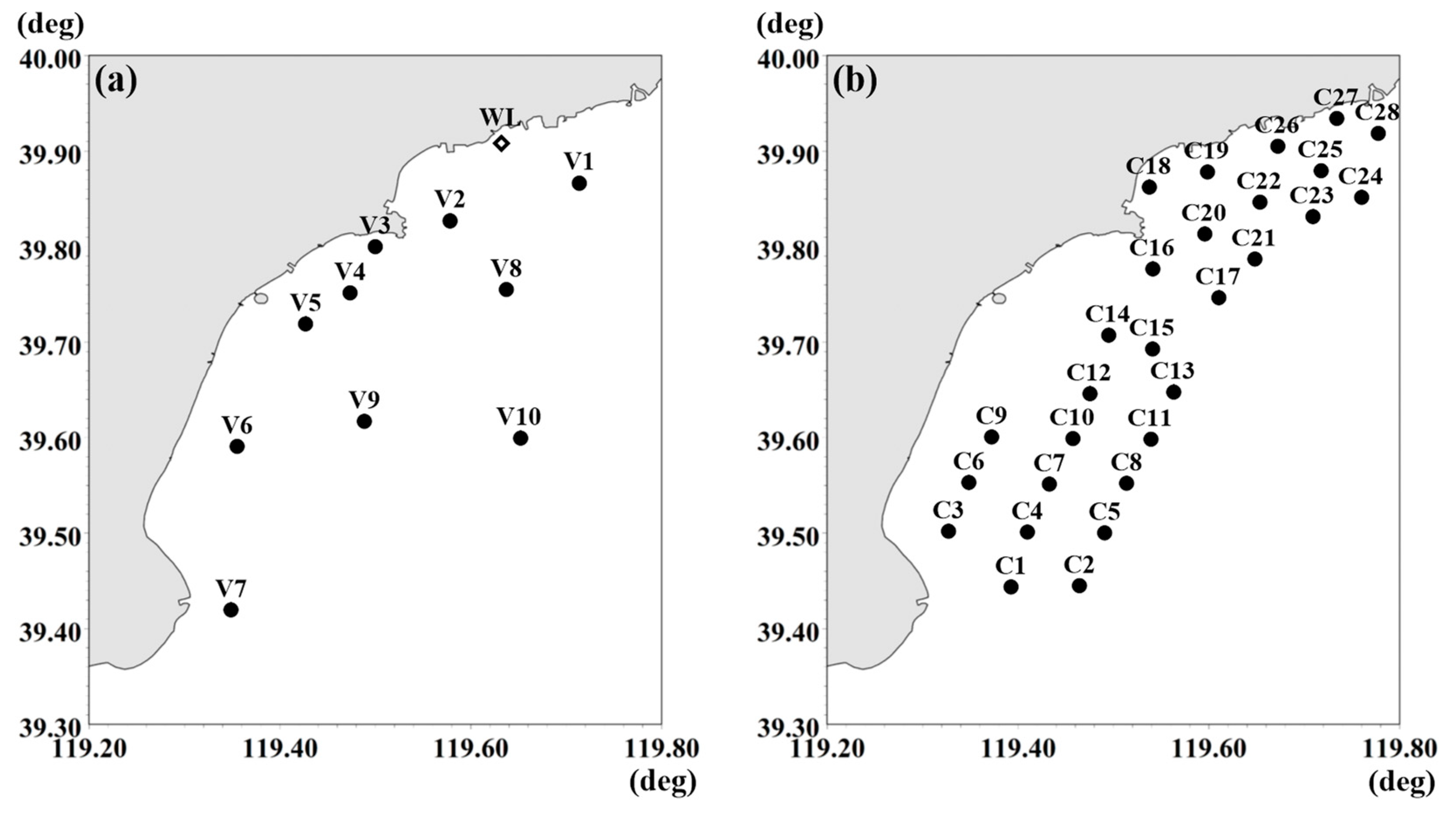
Predicted and observed water level and current were compared with each other to assess the performance of the hydrodynamic model. The hydrodynamic measurement work in May of 2013 was for other coastal projects by the Marine Environmental Monitoring Center of Hebei Province Qinhuangdao, China. However, measurements from July to August when the largest runoff occurs would be better for calibrating the model. Observations at 10 current stations (V1–V10) and 1 water level station (WL), as indicated in Figure 2a, provided measurements from 0:00 on 11 May to 24:00 on 12 May and from 0:00 on 16 May to 24:00 on 17 May 2013. The water level was measured at the tide station near XKH estuary based on the limnimeter (DCX-22, Keller, Zug, Switzerland). For current observation, 10 stations with an acoustic Doppler current profiler (ADCP) were set in QHD coastal area, and vertical mean current speed and direction were adopted. The observed COD concentrations given by the sampling laboratory report of 28 observation stations (C1–C28), as shown in Figure 2b, were used to validate the water quality model. The water samples were collected on 11 August 2013 and brought back to the laboratory for determination of the permanganate index (CODMn). The runoff was measured once a month in every seagoing river by a flowmeter in 2013; in the same manner, the water was sampled for determination of the dichromate index (CODCr) which was converted into CODMn as the river boundary. In this study, CODMn is treated as the major water quality research object and is uniformly called COD concentration in later sections.
3.3. Model Validations
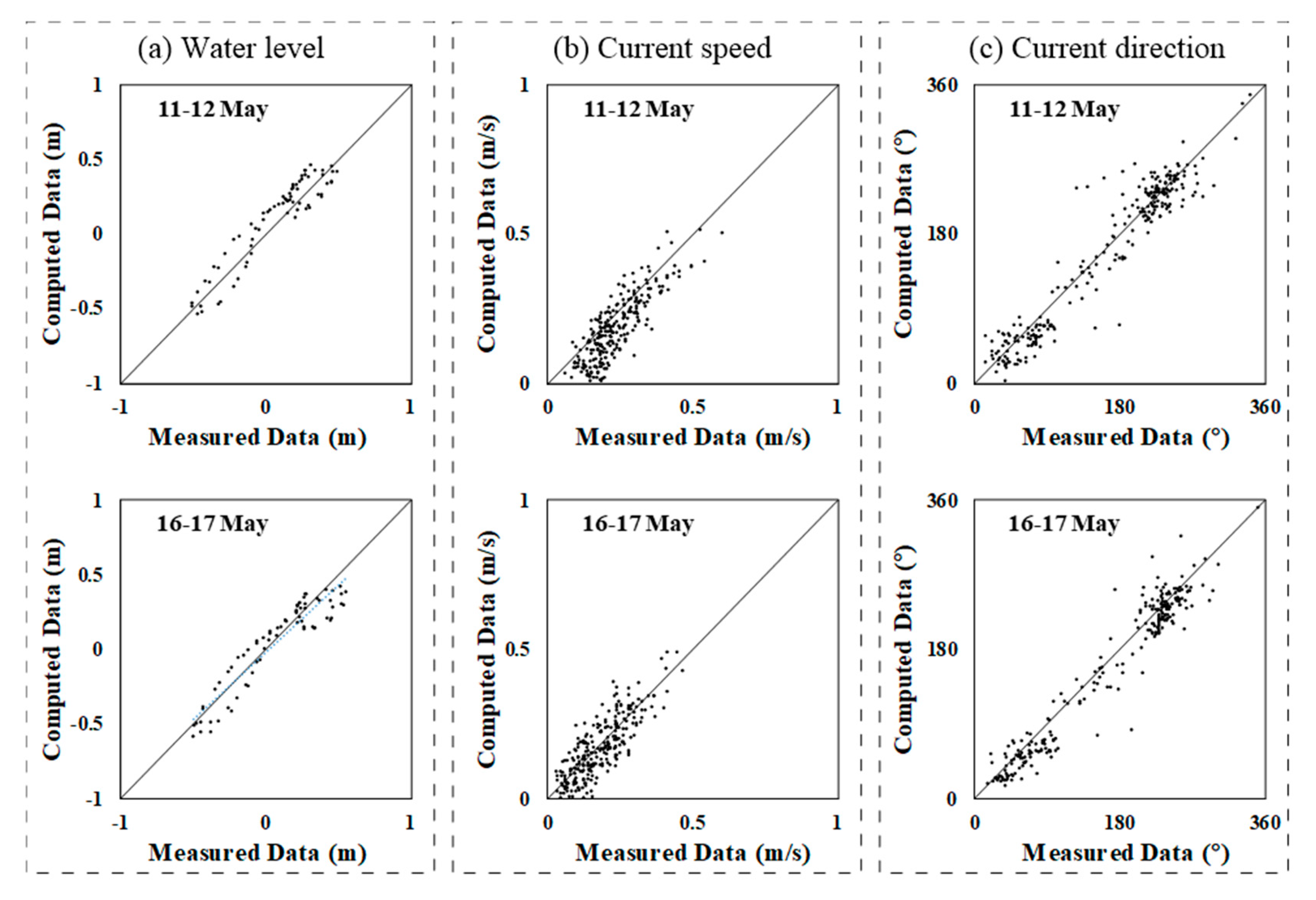
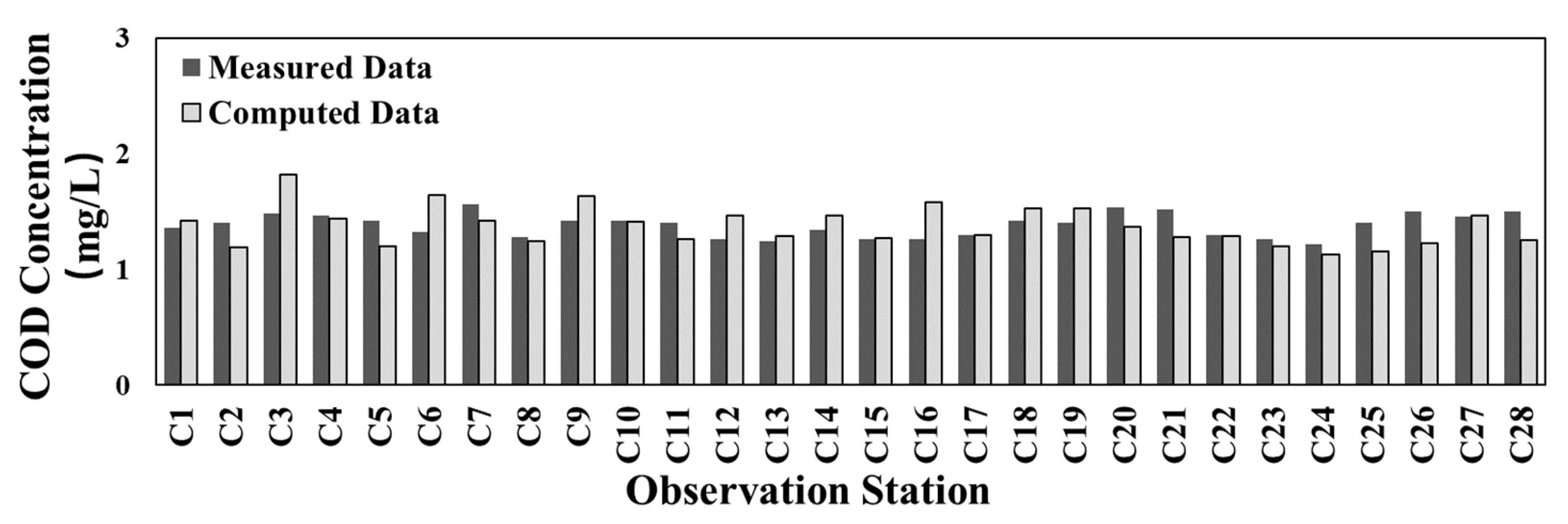
A favorable linear correlation between measured and model predicted COD concentrations confirmed the good agreement between the model and data. R2 was used to quantify the model–data agreement in the range of 0 to 1 (i.e., if R2 was close to 1, the correlation was higher). Figure 3 indicates good agreements between the measured and computed water level, current speed, and current direction. The R2 values were 0.80 and 0.87 for the computed and observed water level, 0.80 and 0.77 for current speed, and 0.94 and 0.92 for current direction on 11–12 May and 16–17 May, respectively. Except for the current speed on 16–17 May, all R2 values were larger than 0.80, which indicates good performance of the hydrodynamic model, even though the hydrodynamic conditions in the QHD sea were complicated and variable due to the presence of an amphidromic point in this region. As shown in Figure 4, the computed and measured COD concentrations compare well. The differences between measured COD concentration once a day and daily average computed COD concentration were acceptable. The water quality model performance of COD concentration was evaluated by the root mean square error (RMSE) [41]. The RMSE of COD concentration was 0.17 mg/L, which indicated that an accurate COD concentration could be obtained from the validated TMAL model.
3.4. Model Results of Total Maximum Allocated Load (TMAL)
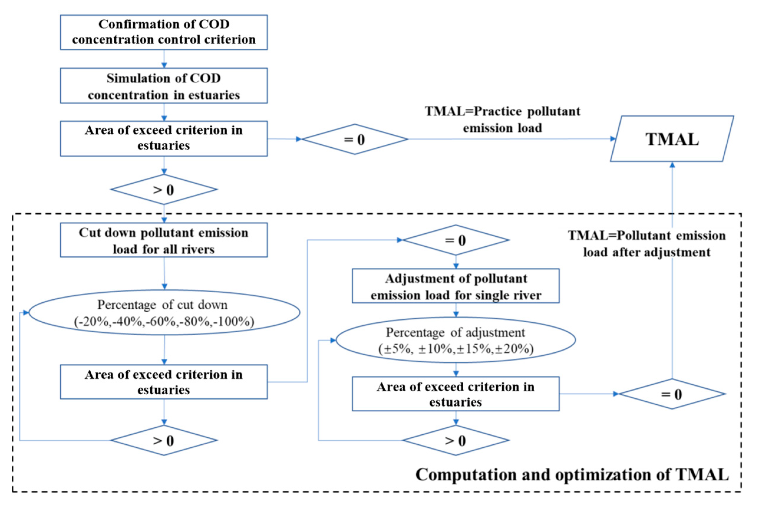
TMAL was determined by source of pollution and water quality distribution characteristics. Due to significant spatial variation of water quality in the QHD sea, it was necessary to execute the computation of the TMAL for each river. As shown in the computational procedure of the TMAL in Figure 5, COD was selected as the focus of this study, and it was necessary to impose an upper limit of COD concentration. The COD concentration control criterion of 2.0 mg/L was empirically determined by the water quality criteria. Based on the model simulation of COD concentration in the QHD sea, the area where the criterion exceeded in estuaries was identified. If no area exceeded the criterion, the TMAL was treated as the good practice pollutant emission load. Otherwise computation of TMAL needed to be determined through an optimization process by cutting down the pollutant emission load. The COD discharge at each river mouth boundary was determined through trial and error (i.e., with a reduction of −20%, −40%, −60%, −80%, and −100% for all rivers successively). If the reduction proportion could not satisfy the water quality criterion, a stronger cut of COD discharge would be adopted until that led to zero areas exceeding the criterion. Then an adjustment process of COD emission load for a single river could improve the accuracy of TMAL. The pollutant emission loads needed to be further decreased for rivers with relatively large pollutant discharge, meanwhile, the loads could be increased for less polluted rivers by ±5%, ±10%, ±15%, and ±20%. When the COD concentration started to exceed the control criterion, TMAL was the pollutant emission load after adjustments using the optimization scheme.
4. Model Results
4.1. COD Transport in Qinhuangdao Sea
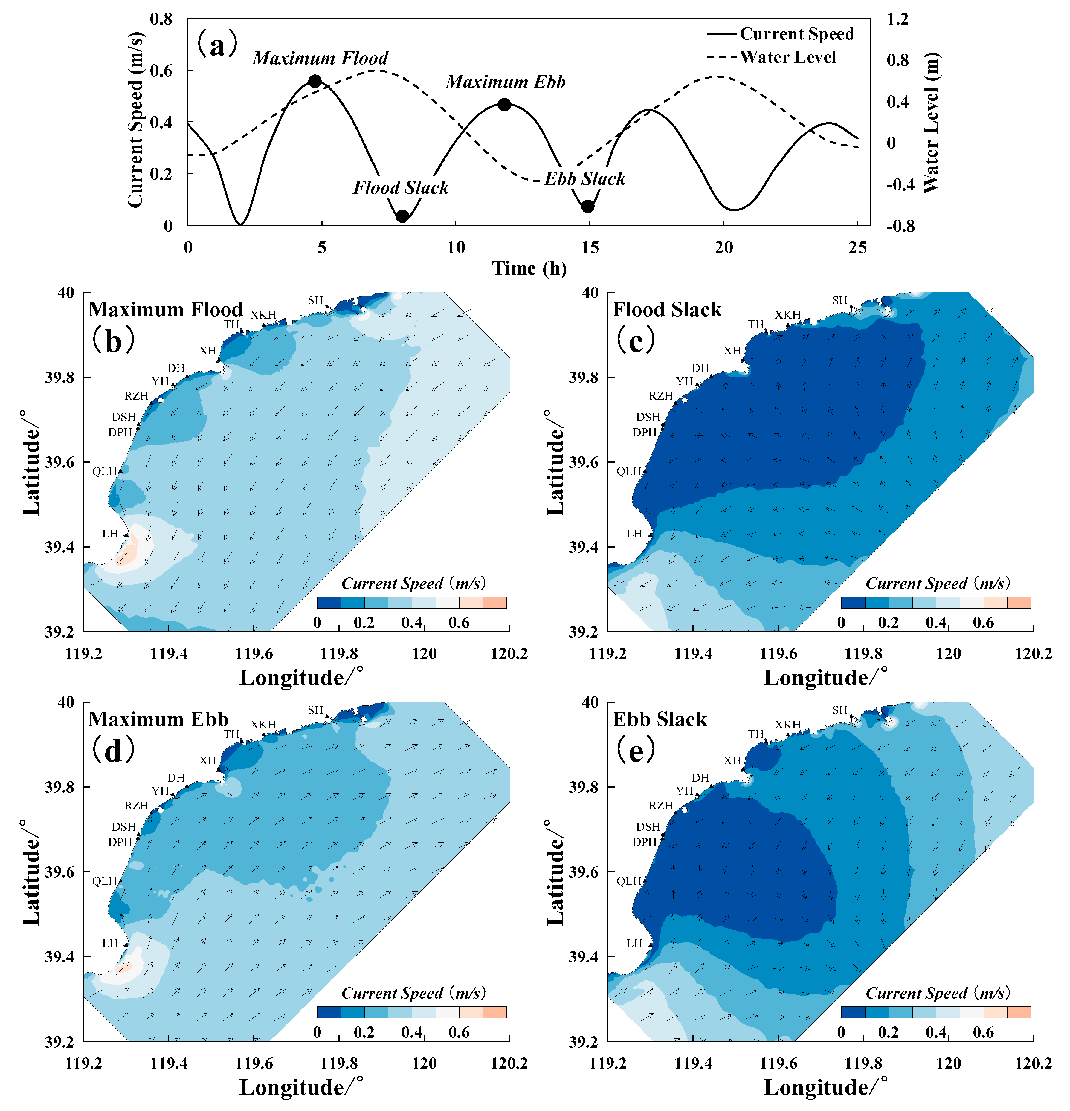
A coupled hydrodynamic and water quality numerical model was validated against field observations. The model was used to simulate hydrodynamics and COD concentrations of the QHD sea in 2013, which supplemented data for large-scale distribution of COD concentration. TMAL was calculated based on the COD concentration distribution which was dominated by tidal current forcing. The variations of water level and current speed near YH estuary (39°46′ N, 119°28′ E) are shown in Figure 6a. The regular semi-diurnal tide shows two peaks and two minima during a daily tidal cycle; however, the hydrodynamics were complicated at the QHD sea, due to approximation to the amphidromic point and the fact that the reversal of the tidal current lagged behind the reversal of the water level [42]. The four typical moments of tidal current were described as maximum flood, flood slack, maximum ebb, and ebb slack, and the flow fields of typical moments are shown in Figure 6b–e. The current was reciprocating flow parallel with coastline and the current direction was west-southwest as flood tide and east-northeast as ebb tide. The current speed magnitude was relatively smaller with inconspicuous differences between flood tide and ebb tide. The average current speed was 0.13~0.3 m/s during flood tide and 0.14~0.32 m/s during ebb tide. At the moment of maximum flood and maximum ebb, the current speeds of the coastal area were smaller than those of open sea, and the current speeds near the LH estuary were relatively larger with 0.4~0.6 m/s. At the moment of flood slack, the current speed near YH and DH estuary was close to 0 m/s, but the current near LH estuary was still flood tide, and the current in the north of the QHD sea was ebb tide. At the moment of ebb slack, the current in the north of QHD sea was flood tide and near LH estuary was ebb tide. It meant that turns of tidal current were not at the same time in spatial distribution of QHD sea; the turns of the tidal current in the north area were in advance of the south area.
In the water quality model, the COD variation in QHD was combined with monthly hydrodynamic conditions and COD discharge at river boundaries. A favorable water exchange capacity helps to alleviate water pollutants and strong tidal stream energy indicates rapid water exchange [43]; therefore, the kinetic energy was derived from the current speed to analyze its influence on water quality distribution.
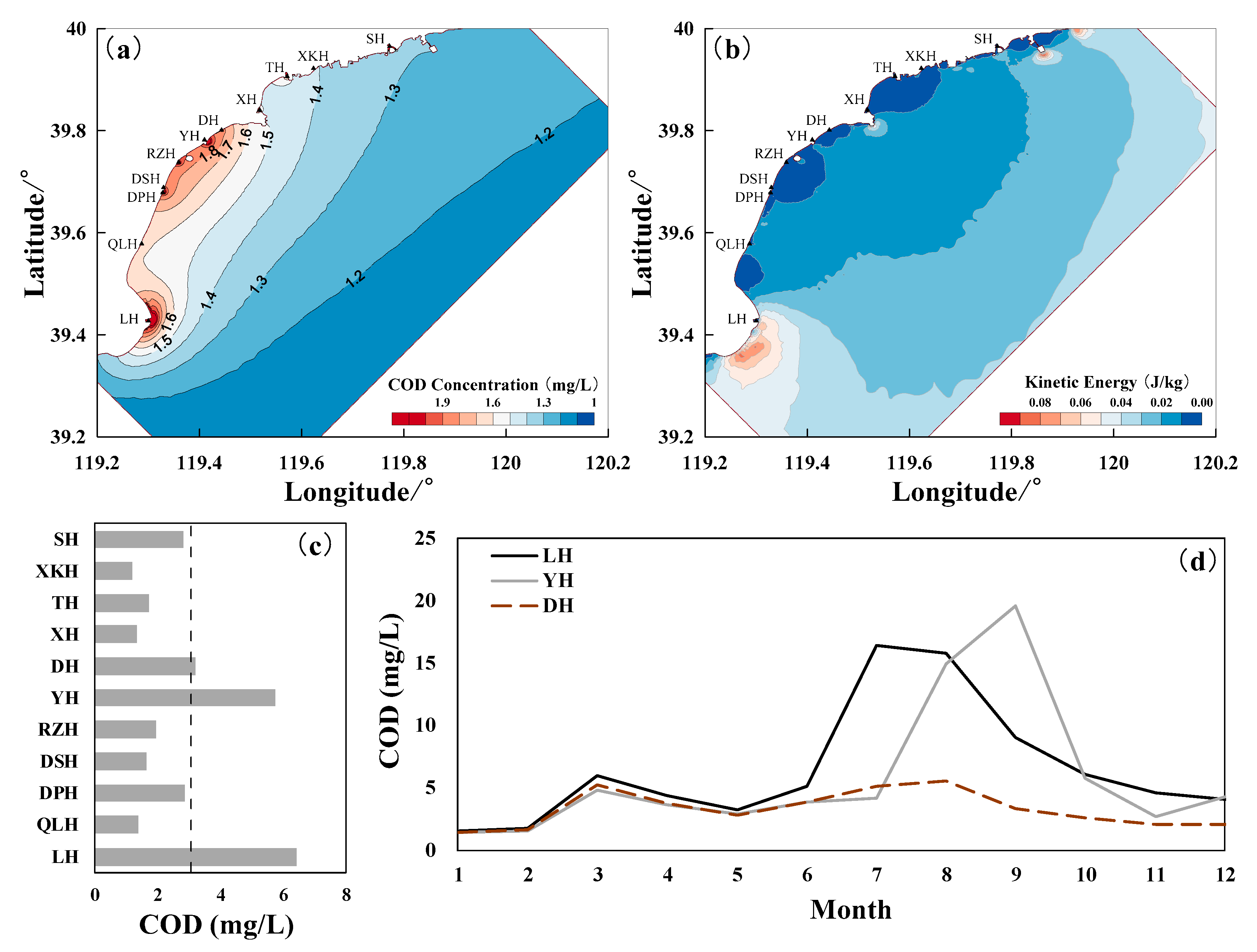
The spatial distributions of annual average COD concentration and annual average kinetic energy for 2013 are shown in Figure 7a,b. The COD concentration in the nearshore was higher than that in the offshore and it was higher in the southwest than northeast of QHD coastal water. It is evident from Figure 7a that isoline of 1.8 mg/L mainly appeared at the coast next to LH and from DPH to DH, while in other areas, the COD concentration was less than 1.8 mg/L. Serious pollution concentrated along the coast between LH and DH. The annual average COD concentrations for the 11 estuaries are shown in Figure 7c, and the COD concentrations of LH, YH, and DH estuaries were larger than 3.0 mg/L and exceeded the criterion of second category water quality. The COD concentration of LH estuary with about 6.4 mg/L in 2013 was the highest among the seagoing rivers in QHD. The COD concentrations at YH and DH were 5.7 mg/L and 3.2 mg/L, respectively. The water quality at DPH was close to the criterion of the second category with COD concentration of 2.8 mg/L. While the COD concentrations of RZH and DSH were lower than 2 mg/L, due to the shorter distance with YH, DH, and DPH, the coastal environment from DPH to DH was severely polluted. The COD concentration of XKH estuary was the lowest at 1.4 mg/L which showed fewer pollutant emissions, and the concentrations of TH, XH, and QLH were lower than 2 mg/L. COD in QLH coastal water was larger than 1.6 mg/L, which was mainly polluted by adjacent estuaries. From the perspective of mean kinetic energy distribution (Figure 7b), the kinetic energies in the southwest and northeast of QHD sea and open sea were relatively larger than those in the nearshore from LH to SH. Except for LH, QLH, and SH, the kinetic energies in adjacent water areas were lower than 0.01 J/kg, which meant a weaker coastal water exchange capacity in the QHD coastal area. Although SH had a larger COD concentration of 2.8 mg/L in estuary, a stronger kinetic energy with 0.025 J/kg led to cleaner water in the adjacent sea.
The three estuaries of LH, YH, and DH had COD concentrations over the second category water quality criterion and were chosen as the case study estuaries to investigate the monthly variation of COD concentrations, as shown in Figure 7d. Winter consists of December, January, and February in QHD, and as the temperature is lower than ice point, the rivers are frozen so that there is rarely any runoff discharge into the sea and pollutant is not liable to be carried by runoff. The COD concentrations of three estuaries in December were larger than those in January and February because rivers were just beginning to freeze in December. There were two peaks in the monthly variation for LH, YH, and DH. The first peak appeared in March and the second peak appeared from July to September. As spring was coming and temperature became warmer in March, accumulation of pollutant from melting ice discharged into the sea and COD concentration increased in each estuary. Although the COD concentration dropped down in April and May because the accumulative effect of pollutant was taped down during March. The precipitation during summer and autumn in QHD was larger than other seasons according to historical meteorological and hydrological data, so that there were larger amounts of water and agricultural pollution discharged during these seasons. Summer was from June to August and autumn was from September to November. The largest COD concentration occurred in July with a magnitude of 16.4 mg/L in LH, in September with a magnitude of 19.6 mg/L in YH, and in August with a magnitude of 5.5 mg/L in DH. Though the COD discharge of LH at 3.28 kg/s in July was larger than that of YH at 2.93 kg/s in September, the maximum COD concentration among the estuaries occurred in YH estuary in September, which was mainly due to the larger kinetic energy of LH estuary than that of YH estuary, as shown in Figure 7b. Therefore, the COD concentration in an estuary was not only controlled by emission load, but also by kinetic energy.
4.2. Water Environmental Capacity and Total Capacity Control of COD
QHD sea is a major tourist attraction for sea baths, therefore, it needs to meet the criterion of second category water quality, so that the COD concentration should be less than or equal to 3.0 mg/L. During red tide outbreaks in Xiamen, COD concentration may exceed 2.0 mg/L [44]. In previous studies of environmental capacity for Luoyuan Bay and Leqing Bay, the COD concentration of 2.0 mg/L was used as the environmental control criterion [45,46]. In QHD sea, before the red tide event in 2011, the COD concentrations of most field stations were lower than 2.0 mg/L, however, more than half of the field observed that COD concentrations became larger than 2.0 mg/L during red tide outbreaks. It follows that COD concentration of 2.0 mg/L was adopted as the indicating index for red tide outbreak [47]. Therefore, it was required to maintain COD concentration below 2.0 mg/L in QHD for sustainable socio-economy development and the natural environment, which satisfied the criterion of second category water quality at the same time. In case COD concentrations exceeded 2.0 mg/L, it was necessary to reduce the concentration by further decreasing the pollutant discharge at unqualified rivers while maintaining the emission at the same level for qualified rivers.
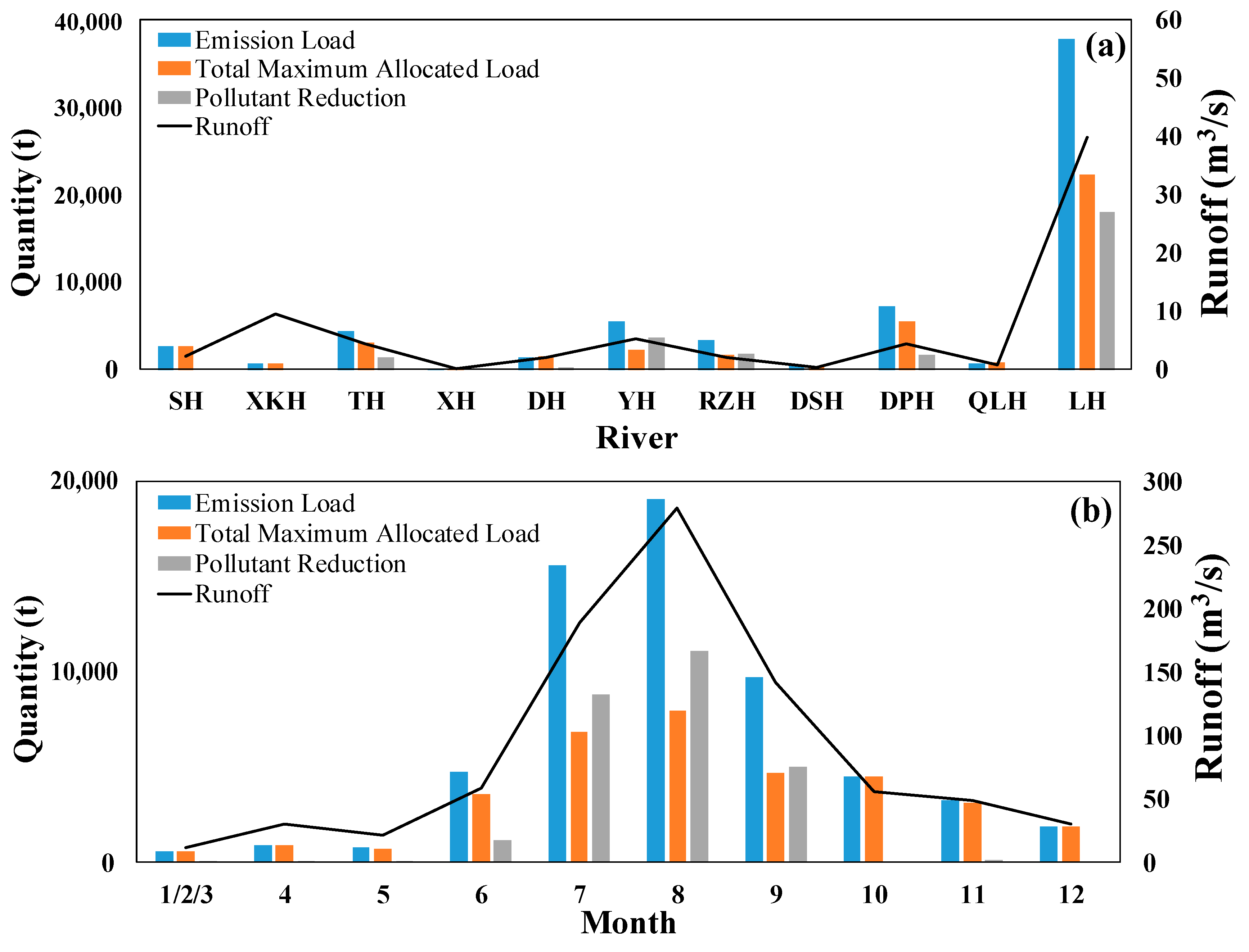
Through simulation of COD concentrations in estuaries and optimization processes, TMAL was calculated for all estuaries every month in 2013. The pollutant reduction was estimated as emission load minus the TMAL that corresponded to the desired total capacity control. The year-round emission load, TMAL, pollutant reduction, and runoff of each seagoing river in 2013 are demonstrated in Figure 8a. Annual mean runoff of LH was the largest at 39.74 m3/s; that of other rivers was lower than 5 m3/s, except for XKH and YH which had runoff of 9.53 m3/s and 5.27 m3/s respectively. It was shown that LH had the largest emission load of 37,817.4 t/a, TMAL of 22,221.3 t/a, and pollutant reduction of 17,993.3 t/a due to the largest runoff. These differences of emission load and TMAL followed the variation of runoff except for XKH which upstream had excellent water quality and little pollutant discharge. Five rivers, SH, XKH, XH, DSH, and QLH, did not need contaminant discharge reduction. Ranking from largest to smallest pollutant reduction was LH, YH, RZH, DPH, TH, and DH, and the effluent discharge of these rivers was necessary to be controlled.
Hydrological characteristics in QHD featured significant seasonal variations due to ephemeral rivers. TMAL, emission load, and pollutant reduction of QHD in 2013 were mainly controlled by runoff with strong seasonal variation. Since temperature of QHD in winter was below the frozen point, rivers were almost all covered by ice with little runoff and effluent discharge, so that January, February, and March were combined together as the average value to be considered. As shown in Figure 8b, variation of seasonal runoff characteristics revealed that small amounts of river discharge into the sea were observed for December to May. In summer and autumn, the runoff became larger. In August, the emission load became the largest with 1.9 × 10⁴ t in 2013 with the abundant runoff of 279 m3/s, and the emission load as well as runoff in July occupied second place. In the other months, the emission loads were lower than 1.0 × 10⁴ t, especially in January to May, which were lower than 1.0 × 10³ t. It was remarkable that variation of emission load, TMAL, and runoff had the same tendency. In other words, runoff was the main dominant control factor for pollutant emission and TMAL. The total capacity control, during the rainy season from June to September had pollutant reduction larger than 200 t, and these months became the key months to regulate pollutant emissions.
5. Discussion
5.1. Correlation of TMAL with Forcing Factors
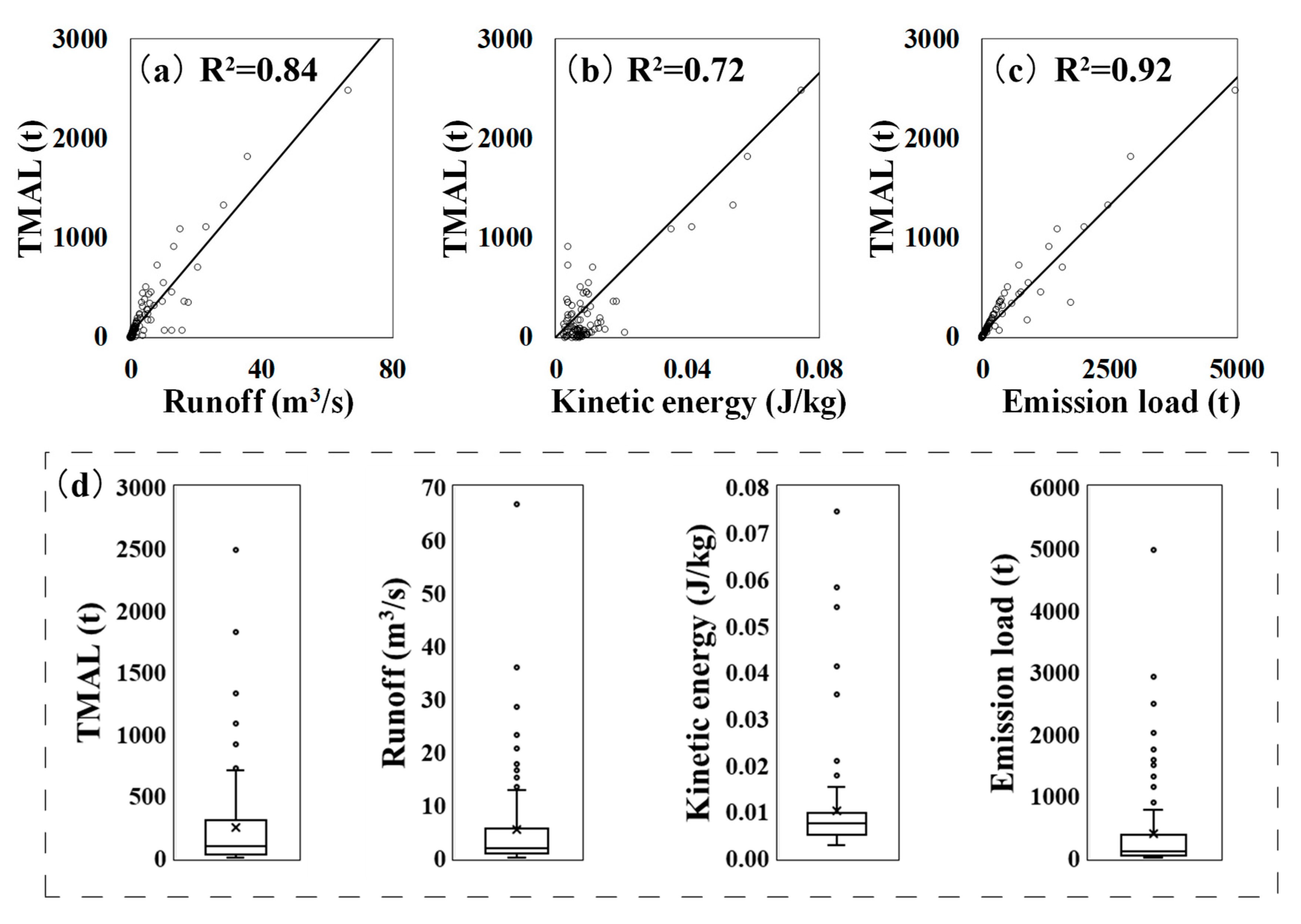
TMAL was calculated by COD concentrations near the estuaries of QHD sea which were controlled by runoff, kinetic energy, and COD discharge. To conduct correlation analysis of various influence factors (runoff, kinetic energy, and emission load) with TMAL, variables including influence factors and TMAL were collected from 11 seagoing rivers every month in 2013. The linear relationships were derived as shown in Figure 9a–c, which suggests that TMAL had approximately linear relationship with these key factors. Emission load featured a particularly high linear correlation with the R2 of 0.92. The R2 values of the correlation of TMAL with runoff and kinetic energy were 0.84 and 0.72, respectively.
Spearman and Pearson coefficients are frequently used to evaluate correlation, whereas the stabilization of Pearson coefficient is influenced by extremum [48]. From the box figure shown in Figure 9d, there were extremums in each factor, therefore the Spearman coefficient was used to evaluate the correlation instead of the Pearson coefficient and the Spearman values are shown in Table 1. The positive value showed the extent of positive correlation. The Spearman value between kinetic energy and runoff was the lowest at 0.84, due to that the current speed in QHD sea was mainly dominated by tide, terrain, and coastline instead of runoff. Similarly, the kinetic energy was mainly controlled by current speed rather than emission load, so that the Spearman value of kinetic energy with emission load was relatively small at 0.85. The Spearman value of 0.88 between kinetic energy and TMAL showed kinetic energy had a significant influence on TMAL. It was evident that runoff had a close correlation with emission load and TMAL with Spearman values at 0.96 and 0.92, respectively. Runoff contributed to pollutant discharge for emission load, meanwhile it could also accelerate pollutant dispersion and increase TMAL. Runoff became the key link between emission load and TMAL with Spearman value of 0.95.
5.2. Environmental Capacity Management
Comprehensive coastal environment and pollution treatment programs of seagoing rivers have been carried out by the QHD municipal government since 2012 [49]. Since March 2012, about 254 companies with illegal pollution discharge and 25 outdated production lines have been shut down. Among them, 167 companies were closed permanently, and 87 companies suspended productions [50]. To assess the effectiveness of management projects on seagoing rives, the emission load, TMAL, and pollutant reduction of COD in 2011 were calculated and compared with those in 2013, as shown in Figure 10. The emission loads of 11 rivers in 2013 were lower than those in 2011, which indicated that the pollutant discharge was mitigated to a certain degree. TMALs in 2013 differed from those in 2011 due to different hydrodynamic conditions in these years; however, TMAL of XKH in 2013 differed from that in 2011 due to pollutant discharge variation. The TMAL of LH in 2013 was larger than that in 2011, mainly due to a larger annual mean runoff of LH at 45.66 m3/s in 2013 than that at 39.74 m3/s in 2011. SH and DH no longer required pollutant reduction, and recommended pollutant reductions of DPH and TH decreased from 2011 to 2013. The total emission load dropped down to 64,272 t in 2013 which was about 83% of that in 2011. Overall, the water environment improved significantly through upstream pollutant control. In recent years, the upstream control program such as the River Governor System, which allocates the supervision and management of river water quality to a particular person in QHD, has improved water qualities in QHD sea and adjacent bathing beaches to satisfy the second category water quality criterion [51]. Reduction of pollutants discharged into the sea from rivers is the key for coastal pollution control and marine disaster prevention.
The environmental capacity and total capacity control of COD was investigated based on hydrologic and water quality field observational data collected once a month. During the model simulation setup, however, the data measured once a month were regarded as the monthly average data. Therefore, construction of monitoring stations was recommended to continuously monitor the discharge and water quality of seagoing rivers, which was adopted by the local government as a pilot project. This monitoring system could measure the water quality in the estuaries of SH, XKK, TH, DH, YH, RZH, DPH, and XKH, and provided sufficient and timely data for future total pollutant capacity control.
6. Conclusions
Premium water quality at Qinhuangdao (QHD) sea in the Bohai Sea is necessary for recreational sea bathing activities, therefore, pollutant management projects have been implemented to improve environmental capacity in this region. In this study, a coupled hydrodynamic and water quality model was constructed to assess water environmental capacity in QHD sea, after model validation with field measurements of tide, current, and water quality. Spatial and monthly temporal variations of COD concentration from 11 rivers to QHD sea were investigated through model simulation for 2013 using MIKE. Total maximum allocated load (TMAL) was derived from the predicted COD concentration and optimized by adjusting the pollutant emission load.
It was found that runoff was the most influential driving factor for pollutant emission load, water environmental capacity, and total pollution capacity control. The seasonal variation of COD indicated that water quality was particularly problematic during the rainy season of summer and autumn when the runoff was at the peak, but less so during winter when rivers were frozen, and less water and pollutant were discharged into the sea. Spearman correlation coefficient results indicated a linear relationship between TMAL and forcing factors such as runoff, kinetic energy, and emission load. Comparisons of TMAL, emission load, and pollutant reduction at QHD Sea in 2011 and 2013 indicated that the upstream pollutant control management scheme such as River Governor System improved coastal water quality significantly. Similar practice may be applied to other coastal areas. Meanwhile, based on previous investigations of environmental capacity, a continuous monitoring system was adopted, and a pilot project is in operation to collect a large data set to achieve more accurate total capacity control.
Author Contributions
Conceptualization, C.K. and J.G.; methodology, Z.D. and C.K.; validation, Z.D.; investigation, Z.D. and C.K.; data curation, Z.D. and J.Z.; observation, J.Z., H.L. and L.Z.; writing—original draft preparation, C.K., Q.Z. and Z.D.; writing—review and editing, C.K., Q.Z. and Z.D.; supervision, C.K. and J.G. All authors have read and agreed to the published version of the manuscript.
Funding
This research was funded by the National Key Research and Development Project of China, grant number 2019YFC1407900, the National Natural Science Foundation of China, grant number 41976159, and the Marine Public Welfare Program of China, grant number 201305003.
Acknowledgments
The authors would like to thank the Eighth Geological Brigade, Hebei Geological Prospecting Bureau, Qinhuangdao, China, Marine Environmental Monitoring Center of Hebei Province Qinhuangdao, China and Jinan University for providing field-measured hydrodynamic and pollutant data that are needed for model validation and result discussion.
Conflicts of Interest
The authors declare no conflict of interest.
Appendix A. Governing Equations of Numerical Model
The numerical models used in this study include hydrodynamic and water quality models. The hydrodynamic model is used to simulate circulation driven by tide and runoff. The governing equations of the hydrodynamic model are continuity Equation (1) and horizontal momentum Equations (2) and (3) as follows:
where is the time; , are the Cartesian co-ordinates; , are the components of depth average current velocity in and direction; is the total water depth with sum of undisturbed water depth and the water level ; is the magnitude of discharge due to point sources and (, ) is the velocity by which the water is discharged into the ambient water; is the Coriolis parameter dominated by the angular rate of revolution and the geographic latitude; is the gravitational acceleration; and are the density and reference density of water; is the atmospheric pressure; and are components of the bottom stresses dominated by bottom roughness; and are horizontal stress terms dominated by sub-grid scale horizontal eddy viscosity [52].
The transport of pollutant variables that are present in the water column is simulated by advection-dispersion process based on water quality and the hydrodynamic model. The transport equation for water quality model is obtained as follows:
where is the depth average concentration; is the horizontal diffusion term; is the linear decay rate; is the concentration of source discharge.
References
- Cracknell, A.P.; Rowan, E.S. Physical Processes in the Coastal Zone: Computer Modelling and Remote Sensing; CRC Press: Boca Raton, FL, USA, 1989; Volume 49, p. 86. [Google Scholar]
- Anderson, D.M. Toxic red tides and harmful algal blooms: A practical challenge in coastal oceanography. Rev. Geophys. 1995, 33, 1189–1200. [Google Scholar] [CrossRef]
- Heisler, J.; Glibert, P.M.; Burkholder, J.M.; Anderson, D.M.; Cochlan, W.; Dennison, W.C.; Dortch, Q.; Gobler, C.J.; Heil, C.A.; Humphries, E. Eutrophication and harmful algal blooms: A scientific consensus. Harmful Algae 2008, 8, 3–13. [Google Scholar] [CrossRef] [PubMed] [Green Version]
- Liu, L.; Zhou, J.; Zheng, B.; Cai, W.; Lin, K.; Tang, J. Temporal and spatial distribution of red tide outbreaks in the Yangtze River Estuary and adjacent waters, China. Mar. Pollut. Bull. 2013, 72, 213–221. [Google Scholar] [CrossRef] [PubMed]
- Deng, Y.; Zheng, B.; Fu, G.; Lei, K.; Li, Z. Study on the total water pollutant load allocation in the Changjiang (Yangtze River) Estuary and adjacent seawater area. Estuar. Coast. Shelf Sci. 2010, 86, 331–336. [Google Scholar] [CrossRef]
- Wang, S.; Li, K.; Liang, S.; Zhang, P.; Lin, G.; Wang, X. An integrated method for the control factor identification of resources and environmental carrying capacity in coastal zones: A case study in Qingdao, China. Ocean Coast Manag. 2017, 142, 90–97. [Google Scholar] [CrossRef]
- Pravdić, V.; Juračić, M. The environmental capacity approach to the control of marine pollution: The case of copper in the Krka River Estuary. Chem. Ecol. 1988, 3, 105–117. [Google Scholar] [CrossRef]
- Zhang, Y.L.; Liu, P.Z. Comprehensive Manual of Water Environmental Capacity; Tsinghua University Press: Beijing, China, 1991; p. 1222. [Google Scholar]
- Miharja, M.; Arsallia, S. Integrated Coastal Zone Planning Based on Environment Carrying Capacity Analysis. Proc. IOP Conf. Earth Environ. Sci. 2017, 79, 012008. [Google Scholar] [CrossRef]
- Wu, J.; Wang, Z. The turn-over and self-cleaning capability of seawater in Dalian Bay. Mar. Sci. 1983, 7, 32–35. [Google Scholar]
- Gu, J.; Hu, C.; Kuang, C.; Kolditz, O.; Shao, H.; Zhang, J.; Liu, H. A water quality model applied for the rivers into the Qinhuangdao coastal water in the Bohai Sea, China. J. Hydrodyn. 2016, 28, 905–913. [Google Scholar] [CrossRef]
- Lopes, J.F.; Dias, J.M.; Cardoso, A.C.; Silva, C. The water quality of the Ria de Aveiro lagoon, Portugal: From the observations to the implementation of a numerical model. Mar. Environ. Res. 2005, 60, 594–628. [Google Scholar] [CrossRef]
- Yassuda, E.A.; Davie, S.R.; Mendelsohn, D.L.; Isaji, T.; Peene, S.J. Development of a waste load allocation model for the Charleston Harbor estuary, phase II: Water quality. Estuar. Coast. Shelf Sci. 2000, 50, 99–107. [Google Scholar] [CrossRef]
- Yan, R.; Gao, Y.; Li, L.; Gao, J. Estimation of water environmental capacity and pollution load reduction for urban lakeside of Lake Taihu, eastern China. Ecol. Eng. 2019, 139, 105587. [Google Scholar] [CrossRef]
- Wang, Q.; Liu, R.; Men, C.; Guo, L.; Miao, Y. Temporal-spatial analysis of water environmental capacity based on the couple of SWAT model and differential evolution algorithm. J. Hydrol. 2019, 569, 155–166. [Google Scholar] [CrossRef]
- Guyondet, T.; Comeau, L.A.; Bacher, C.; Grant, J.; Rosland, R.; Sonier, R.; Filgueira, R. Climate change influences carrying capacity in a coastal embayment dedicated to shellfish aquaculture. Estuar. Coast 2015, 38, 1593–1618. [Google Scholar] [CrossRef] [Green Version]
- Wang, H.Y.; Deng, J.; He, K.; Wang, Z.H. Regulation Based on the Carrying Capacity of the Water Environment and Water Quality Information System Model Research. Adv. Mater. Res. 2013, 610–613, 936–940. [Google Scholar] [CrossRef]
- Waltham, N.J.; Elliott, M.; Lee, S.Y.; Lovelock, C.; Duarte, C.M.; Buelow, C.; Simenstad, C.; Nagelkerken, I.; Claassens, L.; Wen, C.K. UN Decade on Ecosystem Restoration 2021–2030—What Chance for Success in Restoring Coastal Ecosystems? Front. Mar. Sci. 2020, 7, 71. [Google Scholar] [CrossRef] [Green Version]
- Zhang, Q. Synthesis of nutrient and sediment export patterns in the Chesapeake Bay watershed: Complex and non-stationary concentration-discharge relationships. Sci. Total Environ. 2018, 618, 1268–1283. [Google Scholar] [CrossRef]
- Kataoka, Y. Water quality management in Japan: Recent developments and challenges for integration. Environ. Policy Gov. 2011, 21, 338–350. [Google Scholar] [CrossRef]
- Hayashi, T. Water pollution control in Japan. J. Water Pollut. Control Fed. 1980, 850–861. [Google Scholar] [CrossRef]
- Tomita, A.; Nakura, Y.; Ishikawa, T. Review of coastal management policy in Japan. J. Coast. Conserv. 2015, 19, 393–404. [Google Scholar] [CrossRef]
- Tomita, A.; Nakura, Y.; Ishikawa, T. New direction for environmental water management. Mar. Pollut. Bull. 2016, 102, 323–328. [Google Scholar] [CrossRef] [PubMed]
- Elshorbagy, A.; Teegavarapu, R.S.; Ormsbee, L. Total maximum daily load (TMDL) approach to surface water quality management: Concepts, issues, and applications. Can. J. Civil Eng. 2005, 32, 442–448. [Google Scholar] [CrossRef]
- Gulati, S.; Stubblefield, A.A.; Hanlon, J.S.; Spier, C.L.; Stringfellow, W.T. Use of continuous and grab sample data for calculating total maximum daily load (TMDL) in agricultural watersheds. Chemosphere 2014, 99, 81–88. [Google Scholar] [CrossRef] [PubMed]
- Huisman, P.; De Jong, J.; Wieriks, K. Transboundary cooperation in shared river basins: Experiences from the Rhine, Meuse and North Sea. Water Policy 2000, 1, 83–97. [Google Scholar] [CrossRef]
- Trela, J.; Płaza, E. Innovative technologies in municipal wastewater treatment plants in Sweden to improve Baltic Sea water quality. Proc. E3S Web Conf. 2018, 45, 113. [Google Scholar] [CrossRef] [Green Version]
- Su, Y.; Wang, X.; Li, K.; Liang, S.; Qian, G.; Jin, H.; Dai, A. Estimation methods and monitoring network issues in the quantitative estimation of land-based COD and TN loads entering the sea: A case study in Qingdao City, China. Environ. Sci. Pollut. Res. 2014, 21, 10067–10082. [Google Scholar] [CrossRef]
- Dai, A.; Li, K.; Ding, D.; Li, Y.; Liang, S.; Li, Y.; Su, Y.; Wang, X. Total maximum allocated load calculation of nitrogen pollutants by linking a 3D biogeochemical–hydrodynamic model with a programming model in Bohai Sea. Cont. Shelf Res. 2015, 111, 197–210. [Google Scholar] [CrossRef]
- Laws, E.; Taguchi, S. The 1987–1989 Phytoplankton Bloom in Kaneohe Bay. Water 2018, 10, 747. [Google Scholar] [CrossRef] [Green Version]
- Lee, Y.S.; Kang, C.K.; Kwon, K.Y.; Kim, S.Y. Organic and inorganic matter increase related to eutrophication in Gamak Bay, South Korea. J. Environ. Biol. 2009, 30, 373–380. [Google Scholar]
- Zhou, Q.; Ma, F.; Zhang, Y.; Zhang, J. Data changes of Buoys during two red tides in Qinhuangdao coastal area after a storm surge. J. Ocean Technol. 2018, 37, 68–73. [Google Scholar]
- Davies, S.; Mirfenderesk, H.; Tomlinson, R.; Szylkarski, S. Hydrodynamic, water quality and sediment transport modeling of estuarine and coastal waters on the gold coast Australia. J. Coast. Res. 2009, SI56, 937–941. [Google Scholar]
- Rothenberger, M.B.; Burkholder, J.M.; Brownie, C. Long-term effects of changing land use practices on surface water quality in a coastal river and lagoonal estuary. Environ. Manag. 2009, 44, 505–523. [Google Scholar] [CrossRef] [PubMed]
- Li, W.; Sun, L.; Cao, X.; Wang, Z. Analysis on temperature variation characteristics of Qinhuangdao in recent 64 Years. J. Environ. Manag. Coll. China 2018, 28, 70–74. [Google Scholar]
- State Council of the People’s Republic of China. The Reply of the State Council on Marine Function Zoning of Hebei Province (2011–2020). Bull. State Counc. People’s Repub. China 2012, 30, 21. [Google Scholar]
- Yang, D.; Zheng, L.; Song, W.; Chen, S.; Zhang, Y. Evaluation indexes and methods for water quality in ocean dumping areas. Procedia Environ. Sci. 2012, 16, 112–117. [Google Scholar] [CrossRef] [Green Version]
- DHI. MIKE 21 & MIKE 3 FLOW MODEL FM Hydrodynamic and Transport Module Scientific Documentation; DHI Group: Hørsholm, Denmark, 2014; p. 52. [Google Scholar]
- Kuang, C.; Liang, H.; Gu, J.; Su, T.; Zhao, X.; Song, H.; Ma, Y.; Dong, Z. Morphological process of a restored estuary downstream of a tidal barrier. Ocean Coast Manag. 2017, 138, 111–123. [Google Scholar] [CrossRef]
- Rodi, W. Turbulence Models and Their Application in Hydraulics; CRC Press: Boca Raton, FL, USA, 1993; p. 124. [Google Scholar]
- Willmott, C.J. On the validation of models. Phys. Geogr. 1981, 2, 184–194. [Google Scholar] [CrossRef]
- Huang, J.; Xu, J.; Gao, S.; Lian, X.; Li, J. Analysis of influence on the Bohai Sea tidal system induced by coastline modification. J. Coast. Res. 2015, 73, 359–363. [Google Scholar] [CrossRef]
- Yang, Z.; Wang, T. Effects of Tidal Stream Energy Extraction on Water Exchange and Transport Timescales. In Marine Renewable Energy; Springer: Berlin/Heidelberg, Germany, 2017; pp. 259–278. [Google Scholar]
- Wu, L. Studies on Relationship of Diatom Red Tides and Environmental Conditions in Tongan Bay. J. Fujian Fish. 2006, 6, 19–23. [Google Scholar]
- Zhang, C. Study on Water Quality and Environmental Capacity in Luoyuan Bay. Master’s Thesis, Ocean University of China, Qingdao, China, 2011. [Google Scholar]
- Huang, X. Study on Marine Environmental Capacity and Total Pollutant Control in Yueqing Bay; Ocean Press: Beijing, China, 2011; p. 418. [Google Scholar]
- Zheng, X.; Fu, Z.; Xi, Y.; Mu, J.; Li, Y. Grey relationship analysis for the environmental factors affecting the Noctiluca scintillans density in Qinhuangdao coastal area. Prog. Fish. Sci. 2014, 35, 8–15. [Google Scholar]
- Myers, L.; Sirois, M.J. Spearman correlation coefficients, differences between. In Wiley StatsRef: Statistics Reference Online; Wiley, 2014; pp. 1–2. Available online: https://www.onacademic.com/detail/journal_1000039512824510_24c6.html (accessed on 15 April 2020).
- Zhang, J.; Cao, X.; Song, X. Investigation and analysis of changes in water quality of major seaward rivers after comprehensive improvement of the offshore environment in Qinhuangdao. Environ. Eng. 2019, 37, 7–11. [Google Scholar]
- Kang, J.; Sun, J.; Zhao, L. Research on the effects and countermeasures of the coastwise environmental comprehensive improvements in Qinhuangdao City. J. Environ. Manag. Coll. China 2015, 25, 39–42. [Google Scholar]
- Song, S. Implement “River Governor System” to improve the ecological condition of all river basins. Hebei Water Resour. 2016, 7, 32–33. [Google Scholar]
- Smagorinsky, J. General circulation experiments with the primitive equations: I. The basic experiment. Mon. Weather Rev. 1963, 91, 99–164. [Google Scholar] [CrossRef]
Figure 1.
(a) Location of the Bohai Sea with the offshore tidal modeling boundary from Dalian to Yantai and Qinhuangdao (QHD) highlighted by the square box; (b) Zoomed-in view of computational mesh of numerical model for QHD and 11 seagoing rivers.
Figure 1.
(a) Location of the Bohai Sea with the offshore tidal modeling boundary from Dalian to Yantai and Qinhuangdao (QHD) highlighted by the square box; (b) Zoomed-in view of computational mesh of numerical model for QHD and 11 seagoing rivers.

Figure 2.
(a) Locations of field observation stations V1 to V10 for velocity and WL for water level; (b) locations of 28 chemical oxygen demand (COD) sampling stations.
Figure 2.
(a) Locations of field observation stations V1 to V10 for velocity and WL for water level; (b) locations of 28 chemical oxygen demand (COD) sampling stations.

Figure 3.
Linear correlation between computed and measured water level, current speed, and current direction on 11–12 May (upper) and 16–17 May (lower) in 2013.
Figure 3.
Linear correlation between computed and measured water level, current speed, and current direction on 11–12 May (upper) and 16–17 May (lower) in 2013.

Figure 4.
Comparison of computed and measured COD concentration at the 28 sampling stations.

Figure 5.
Computation procedures of total maximum allocated load (TMAL) with optimization process based on COD concentration simulation.
Figure 5.
Computation procedures of total maximum allocated load (TMAL) with optimization process based on COD concentration simulation.

Figure 6.
(a) The variations of water level and current speed in a tidal cycle; the flow fields of (b) maximum flood, (c) flood slack, (d) maximum ebb, and (e) ebb slack. Abbreviations: Luanhe River (LH), Qilihai Lagoon (QLH), Dapuhe River (DPH), Dongshahe River (DSH), Renzaohe River (RZH), Yanghe River (YH), Daihe River (DH), Xinhe River (XH), Tanghe River (TH), Xinkaihe River (XKH), and Shihe River (SH).

Figure 7.
(a) The spatial distribution of annual average COD concentration in 2013; (b) the spatial distribution of annual average kinetic energy; (c) the annual average COD concentrations in 11 estuaries in QHD sea; (d) variations of COD concentrations in LH, YH, and DH estuaries where annual mean COD concentration exceeds 3 mg/L.

Figure 8.
(a) The year-round emission load, TMAL, pollutant reduction, and runoff of 11 seagoing rivers in QHD sea in 2013. (b) Monthly average variations of emission load, TMAL, pollutant reduction, and runoff of all rivers in QHD sea during 2013.
Figure 8.
(a) The year-round emission load, TMAL, pollutant reduction, and runoff of 11 seagoing rivers in QHD sea in 2013. (b) Monthly average variations of emission load, TMAL, pollutant reduction, and runoff of all rivers in QHD sea during 2013.

Figure 9.
Linear correlations between (a) runoff, (b) kinetic energy, and (c) emission load and TMAL in 2013; (d) discrete degrees of scattered data of TMAL, runoff, kinetic energy, and emission load.
Figure 9.
Linear correlations between (a) runoff, (b) kinetic energy, and (c) emission load and TMAL in 2013; (d) discrete degrees of scattered data of TMAL, runoff, kinetic energy, and emission load.

Figure 10.
Comparisons of emission load, TMAL, and pollutant reduction of 11 rivers in QHD sea between 2011 and 2013.
Figure 10.
Comparisons of emission load, TMAL, and pollutant reduction of 11 rivers in QHD sea between 2011 and 2013.


Table 1.
Spearman values between TMAL (total maximum allocated load), runoff, kinetic energy, and emission load.
Table 1.
Spearman values between TMAL (total maximum allocated load), runoff, kinetic energy, and emission load.
| Factors | TMAL | Runoff | Kinetic Energy | Emission Load |
|---|---|---|---|---|
| TMAL | 1.00 | 0.92 | 0.88 | 0.95 |
| Runoff | 0.92 | 1.00 | 0.84 | 0.96 |
| Kinetic energy | 0.88 | 0.84 | 1.00 | 0.85 |
| Emission load | 0.95 | 0.96 | 0.85 | 1.00 |
© 2020 by the authors. Licensee MDPI, Basel, Switzerland. This article is an open access article distributed under the terms and conditions of the Creative Commons Attribution (CC BY) license (http://creativecommons.org/licenses/by/4.0/).
Share and Cite
MDPI and ACS Style
Dong, Z.; Kuang, C.; Gu, J.; Zou, Q.; Zhang, J.; Liu, H.; Zhu, L. Total Maximum Allocated Load of Chemical Oxygen Demand Near Qinhuangdao in Bohai Sea: Model and Field Observations. Water 2020, 12, 1141. https://doi.org/10.3390/w12041141
AMA Style
Dong Z, Kuang C, Gu J, Zou Q, Zhang J, Liu H, Zhu L. Total Maximum Allocated Load of Chemical Oxygen Demand Near Qinhuangdao in Bohai Sea: Model and Field Observations. Water. 2020; 12(4):1141. https://doi.org/10.3390/w12041141
Chicago/Turabian StyleDong, Zhichao, Cuiping Kuang, Jie Gu, Qingping Zou, Jiabo Zhang, Huixin Liu, and Lei Zhu. 2020. "Total Maximum Allocated Load of Chemical Oxygen Demand Near Qinhuangdao in Bohai Sea: Model and Field Observations" Water 12, no. 4: 1141. https://doi.org/10.3390/w12041141
Note that from the first issue of 2016, this journal uses article numbers instead of page numbers. See further details here.