Coupling SKS and SWMM to Solve the Inverse Problem Based on Artificial Tracer Tests in Karstic Aquifers


1
Géosciences Environnement Toulouse (GET), CNRS–UPS–IRD–CNES, 14 avenue Edouard Belin, 31400 Toulouse, France
2
Centre of Hydrogeology and Geothermics, University of Neuchâtel, 11 Rue Emile Argand, CH-2000 Neuchâtel, Switzerland
*
Author to whom correspondence should be addressed.
Water 2020, 12(4), 1139; https://doi.org/10.3390/w12041139
Submission received: 9 March 2020
/
Revised: 10 April 2020
/
Accepted: 13 April 2020
/
Published: 16 April 2020
(This article belongs to the Special Issue Recent Advances in Karstic Hydrogeology)
Abstract
:Artificial tracer tests constitute one of the most powerful tools to investigate solute transport in conduit-dominated karstic aquifers. One can retrieve information about the internal structure of the aquifer directly by a careful analysis of the residence time distribution (RTD). Moreover, recent studies have shown the strong dependence of solute transport in karstic aquifers on boundary conditions. Information from artificial tracer tests leads us to propose a hypothesis about the internal structure of the aquifers and the effect of the boundary conditions (mainly high or low water level). So, a multi-tracer test calibration of a model appeared to be more consistent in identifying the effects of changes to the boundary conditions and to take into consideration their effects on solute transport. In this study, we proposed to run the inverse problem based on artificial tracer tests with a numerical procedure composed of the following three main steps: (1) conduit network geometries were simulated using a pseudo-genetic algorithm; (2) the hypothesis about boundary conditions was imposed in the simulated conduit networks; and (3) flow and solute transport were simulated. Then, using a trial-and-error procedure, the simulated RTDs were compared to the observed RTD on a large range of simulations, allowing identification of the conduit geometries and boundary conditions that better honor the field data. This constitutes a new approach to better constrain inverse problems using a multi-tracer test calibration including transient flow.
1. Introduction
Karstic aquifers can be characterized by a hierarchical drainage system embedded in a calcareous matrix having a much lower hydraulic conductivity [1]. The internal structure of karstic aquifers is the result of karstification processes: fracture and bedding planes are enlarged by dissolution, leading to a gradual establishment of a conduit network [2]. The location and the size of the conduits are generally unknown, leading to major issues for the potential application of physically distributed karst models [3]. Although the complete description of flow paths in karstic aquifers is not possible, several methods have been developed to characterize groundwater drainage structure in karstic aquifers, such as artificial tracer tests [4] and applied geophysics [5], among others.
Artificial tracer tests constitute one of the most powerful tools to investigate solute transport in conduit dominated karstic aquifers [6,7,8,9,10,11,12,13]. The careful analysis of the residence time distribution (RTD) derived from the tracer breakthrough curve (BTC) allows getting information about the internal structure of the aquifer. As an example, a tailing effect can be the consequence of the existence of dead space [9,14,15] or friction effects [8]. Otherwise, this could be due to the coexistence of multiple flow dynamics [10,13]. A multiple peaked RTD could give evidence of multiple flow paths in the system [16,17,18]. Besides, the RTD shape may be directly linked to the spatial distribution of flow and transport. Investigations at bench-scale [16,19,20,21] enabled the identification of the effects of different flow patterns on the RTD measured at the outlet of the system. Also, changes in boundary conditions should be considered properly, since they may have a strong influence on the RTD shape [11,12] even on a flood event scale [13]. So, one should consider that the observed RTD is a convolution of the signal transformation made by every part of the system along the solute transport path for a specific range of boundary conditions.
Considering the above-mentioned information, it should be theoretically possible to infer conduit network geometry based on artificial tracer tests [3]. Nonetheless, it constitutes a complex task because one needs to solve several problems with numerical modeling of the conduit network and then about flow and solute transport in a synthetic karst model. Many modeling approaches dealing with solute transport in karstic aquifers have been developed in past decades. As an example, the pipe flow models [22,23] consider the karst aquifer as a horizontal network of pipe connecting points within the aquifer [24,25]. This modeling approach can also be implemented in the Modflow Conduit Flow Processes (CFP) model, allowing the simulation of turbulent and laminar groundwater flow conditions [26] and consideration of lateral exchanges between the conduit and saturated fissured matrix through a dependence between head difference between matrix continuum and discrete conduit [27]. Modflow CFP model has been used to simulate the solute transport in karstic aquifers [28,29], to improve the understanding of the interaction between seawater and freshwater in coastal aquifers [30,31], and to improve the interpretation of artificial tracer tests [32]. Other studies have not considered lateral exchanges and use of the Storm Water Management Model (SWMM) [33], developed by the United States Environmental Protection Agency (EPA). In this approach, the aquifer is considered as an assembly of interconnected pipes without interaction with the surrounding matrix [34,35]. Considering that the conduit geometry in a karst aquifer is well known, the conduit network can be converted in the analogous sewer system with pipes and junctions. In the case where the position and size of the conduit are unknown, one should try to solve the inverse problem based on artificial tracer tests [36].
The main focus of this study consisted of attempting to solve the inverse problems based on artificial tracer tests. So, the objective was to answer whether we can constrain the conduit network geometry using artificial tracer test data. Conduit network geometries were simulated using the Stochastic Karst Simulator (SKS), a pseudo-genetic algorithm [3,37] including field data such as geology and structural heterogeneities. Then, the flow and the solute transport were simulated using the Storm Water Management Model (SWMM). Then, using a systematic search procedure, the simulated RTDs were compared to the observed RTD for a large range of simulations, allowing identification of the conduit geometries and boundary conditions that better match the field data.
2. Materials and Methods
2.1. Study site and Field Data
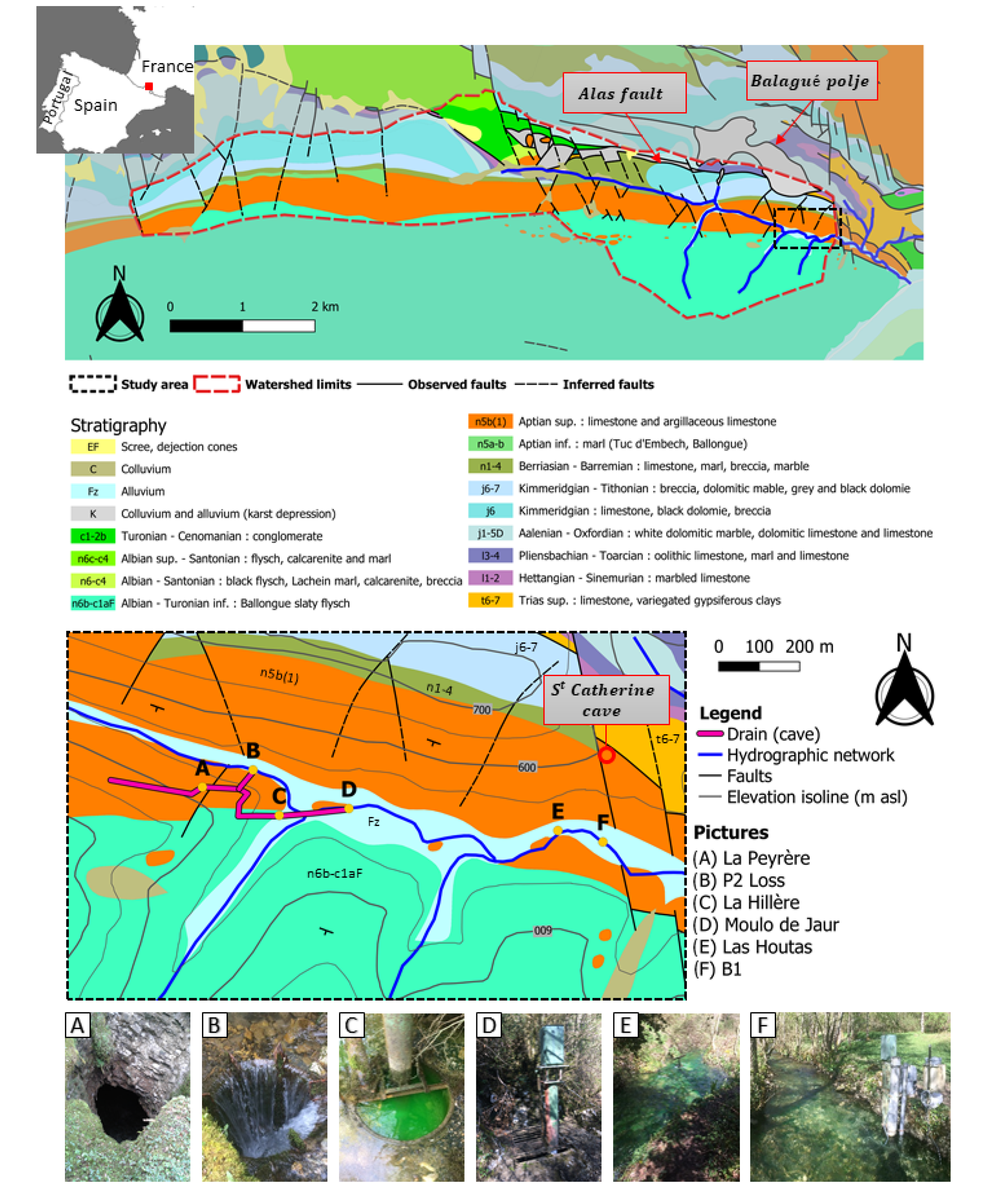
The area studied is the Baget karstic watershed, part of the French KARST observatory network (SNO KARST) [38]. This basin is in the Pyrenees Mountains (Ariège, France) and is characterized by a recharge area of about 13.2 km2 and a median elevation of about 940 m above sea level (a.s.l.). It belongs to the carbonate belt bordering the North of the French Pyrenees (Figure 1). The area was highly deformed during late Cenomanian to Tertiary Pyrenean orogeny induced by the transpressional strike-slip motion of the Iberic and European plates along the North Pyrenean fault [39,40]. The karstified part of the basin is characterized by metamorphic Jurassic to Cretaceous dolomites, limestones and calcareous marls. As a consequence of the metamorphism, matrix porosity was reduced to less than 1 percent [41]. These formations deep 70° to 90° southwards, under the slaty Albian-Cenomanian Ballongue flysch. The southern part of the area consists of a Cretaceous pull-apart basin opened during strike-slip motion along the Pyrenean margin [40,42]. A secondary fault from the North Pyrenean fault, the Alas fault, and the Balagué polje constitute the northern limit of the Baget drainage basin. The contact between the karstified calcareous formations and the impermeable flysch gives the valley orientation in the west-east direction. In the upstream part of the watershed, the Lachein river flows during periods of the high-water level; otherwise, the river flows downstream the perennial spring of the Baget watershed, Las Hountas. The downstream part of the watershed is characterized by the presence of loss and temporary and permanent resurgences on a spatially restrained area of around 1 km2 (Figure 1). According to Mangin [41], voids consist of dissolution caves and in open fractures and joints. Several caves have been recognized and mapped, such as St Catherine, La Peyrère [43] and part of the system between La Peyrère, P2 Loss, and Moulo de Jaur [44]. Several approaches have been performed to attempt to establish voids geometry [45,46] and their influence in solute transport [10,13,41].
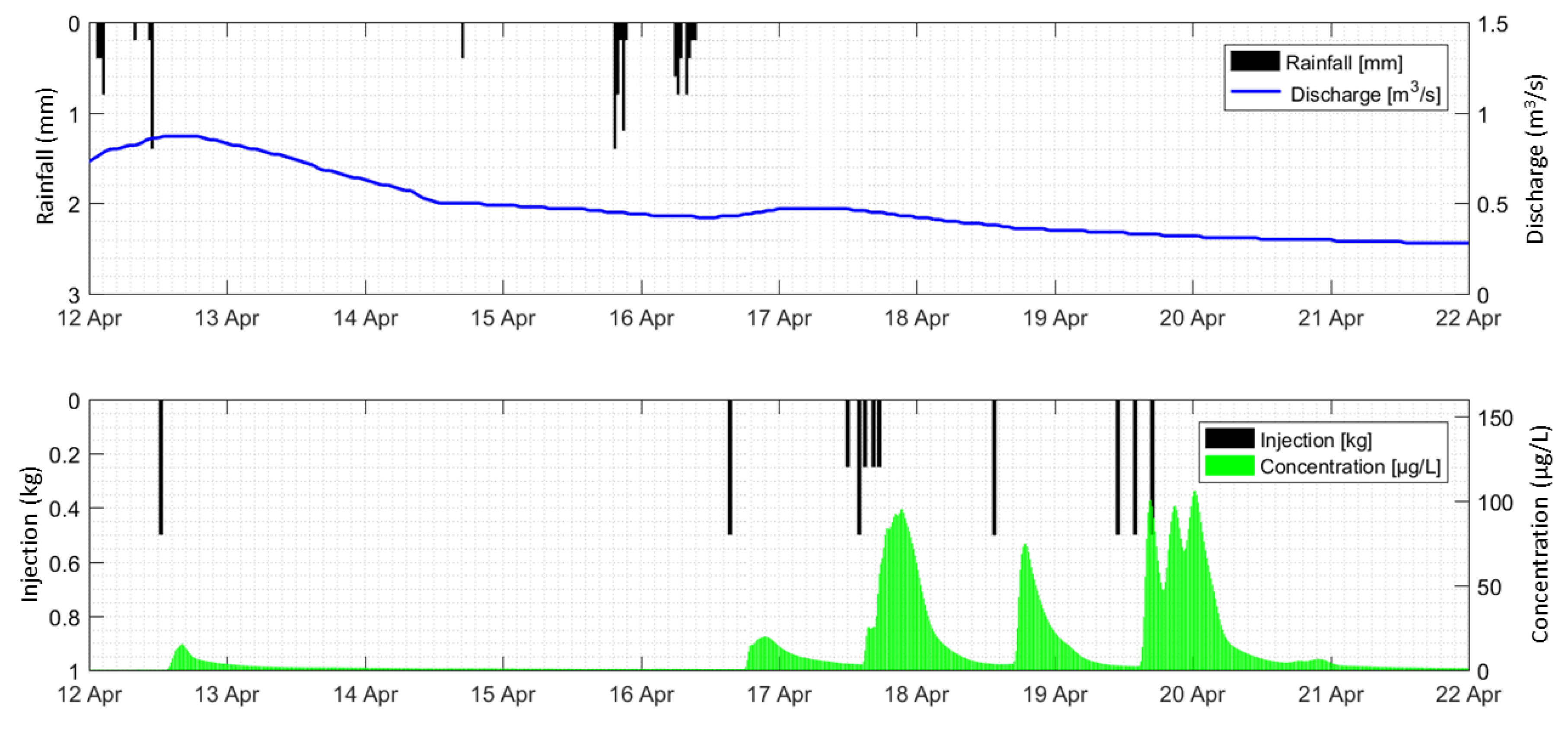
The Baget watershed has been previously studied based on artificial tracer tests [41,47]. Labat and Mangin [10] proposed a transfer function-based interpretation of artificial tracer tests performed from several points of the area (Peyrère, Moulo de Jaur, and P2 Loss) to the perennial resurgence of the Baget watershed, called Las Hountas. The recovery rate was greater than 95% for all tracer tests showing a good hydraulic connection between injection and recovery points. Sivelle and Labat [13] focused on the solute transport between P2 Loss and Las Hountas. Eleven artificial tracer tests were performed on a few days, without any significant influence of rainfall. During, the tracer test campaign, the discharge varied from 0.9 m3/s at the beginning down to 0.3 m3/s at the end of the campaign (Figure 2). A field fluorimeter GGUNFL-30 [48] was installed near the station B1, where the discharge has been measured since the late 1960s [41]. The fluorescence measurement is done on a 15-min sampling rate and the water sampling is performed at an hourly sampling rate. Water samples were analyzed by the CETRAHE laboratory (Orléans, France) using a spectrofluorimeter Hitachi F2500 and F7000. The injection point P2 Loss was chosen so the tracer reached the subterranean drainage system rapidly, getting close from an instantaneous injection (Dirac function).
The effect of short-term variations in discharge on solute transport has been highlighted using a transfer function approach [13]. This constitutes an easily reproducible framework for other systems [49]. Nonetheless, the transfer function approach consists of a systemic approach but does not consider any information about the internal structure of the aquifer.
Applying a physical approach to artificial tracer test interpretation requires a minimum level of knowledge about the flow geometry. One of the most commonly used methods is based on analytical solutions of the advection-dispersion equation (ADE) [50]. The application of such models assumes that both flow and dispersivity are constant along the flow path. This hypothesis is rarely observed in karst media. However, the system studied can be segmented in a sub-structure, called “reach”, where the flow conditions can be considered as homogeneous [12,15,51]. That implies that the underground drainage structure is well known to constrain the physically based modeling [52,53]. In a case where the internal structure is unknown and difficult to access (speleology, cave monitoring), coupling artificial tracer tests and numerical modeling could provide additional information [36]. In this study, the part of the conduit network which has been characterized by the speleological investigation (Figure 1) was considered as conditional data for the simulation of the synthetic conduit networks.
2.2. Modeling Approach
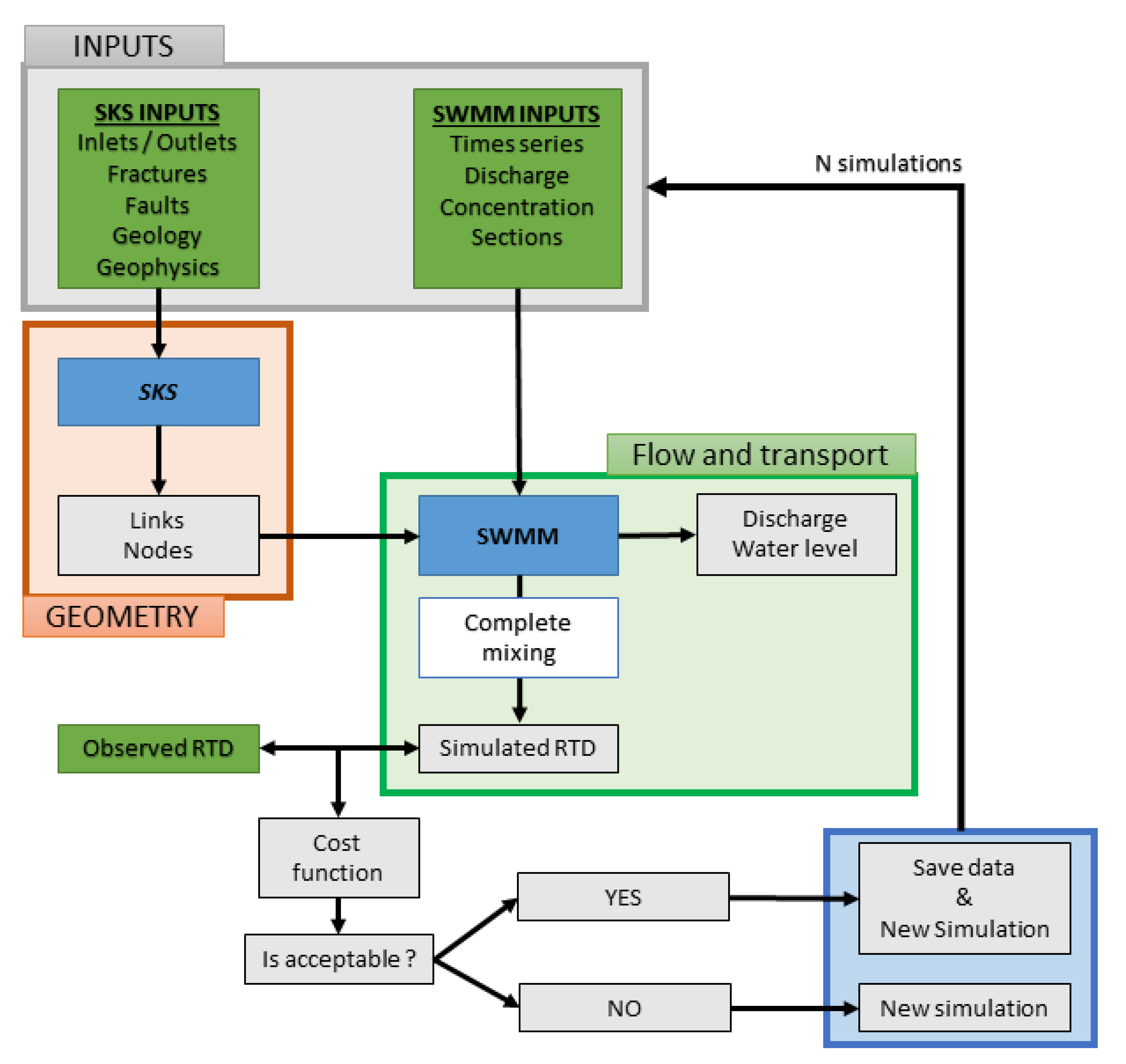
The modeling workflow (Figure 3) was based on a systematic search procedure to solve the inverse problem based on artificial tracer test data. One needs to identify both the conduit geometry and the flow conditions that are at the origin of the RTD measured at the outlet of the system. To do so, synthetic karst networks were simulated using a pseudo-genetic algorithm, then, different plausible flow conditions were applied to simulate flow and solute transport. Finally, the simulated RTD was compared to the observed RTD using the Nash-Sutcliff Efficiency coefficient (NSE) [56]. The procedure was applied to 1000 simulations allowing to identify the geometries and flow conditions that are compatible with the observed RTD.
2.2.1. Conduit Network Simulation
The conduit networks simulation was performed using the Stochastic Karst Simulator (SKS) developed by Borghi et al. [3,37]. The procedure consisted of four main steps:
- Building a geological model of the studied area. It covered about 1 km2. Only the two main geological formations were considered: the slaty flysch in the southern part of the area and the Jurassic to Cretaceous metamorphic limestones in the northern part of the area. The contact between these two formations is oriented in the west-east direction. The calcareous formation was numerically considered as a homogeneous formation affected by structural heterogeneities (faults and fractures). Then, bedding planes, inception horizons, or even foliation were not considered for implementation of geological constraints in conduit networks simulation with SKS. This constitutes a strong hypothesis but seems to be acceptable regarding the small extension of the simulation area. Moreover, slaty formations constituted a boundary condition for the development of the conduit networks.
- The structural heterogeneities (faults and fractures) over the area were considered in the SKS model. The main discontinuity direction was recognized from the satellite image, running 170° N to 10° N orientations [57,58,59] as well as the faults and fractures reported by the French geological survey (BRGM) in the BD_CHARM database [54]. The fracture model includes the main structures identified in the area and a set of stochastic fractures that is different for every simulation and generated following the statistical distributions derived from the field data. Besides, the observations made through speleological investigations [44] have been considered as conditional data in the conduit network simulations; thus, SKS reproduces this known conduit.
- The inlets and outlets can be identified and imposed in SKS. The inlets are composed of La Peyrère, P2 Loss, La Hillière and Moulo de Jaur. Moreover, some additional potential inlets can be randomly added over the area to ensure more physical realism and to allow potential feeding branches along with the solute transport to be considered. Then, Las Hountas, which is the perennial outlet of the Baget system, constitutes the only outlet of the synthetic conduits networks.
Finally, nodes and links were automatically extracted from the synthetic conduit networks and using the Dijkstra algorithm [61] the shortest path between the inlet(s) and outlet(s) can be extracted. So, the tracer path was identified based on the hypothesis that the tracer will be transported through the minimum effort path.
2.2.2. Flow Simulation
The flow simulation in the synthetic conduit networks was performed using the EPA Storm Water Management Model (SWMM) [33]. Considering that there are no lateral exchanges between the simulated conduits and the matrix system, the aquifer can be compared to a set of interconnected pipes [34]. This constitutes a strong hypothesis, but it seems to be acceptable over the Baget area. It was estimated, through a conceptual reservoir model, that the reservoir corresponding to the matrix contributes about 10% in the total spring discharge [62] and the tracer velocity measured by Sivelle and Labat [13] is characteristic of conduit dominated karstic aquifers [63].
To simulate flow, SWMM implements the Saint-Venant equations [64,65] that represent the principles of conservation of momentum and conservation of mass (Equations (1) and (2)).
where is the depth of water (L), is the velocity (L·t−1), is the longitudinal distance (L), is the time (t), is the gravitational acceleration (L·t−2), is the channel slope, is the friction slope, is the area of the flow cross-section and is a function of y upon the geometry of the conduit (L2) and is the discharge with (L3·t−1).
Equation (1) represents hydrostatic pressure, convective acceleration, local acceleration and gravity, and frictional forces, respectively. Representing the effects of turbulence and viscosity, the friction slope () is calculated in SWMM using Manning’s equation [66]:
where is the Manning’s roughness coefficient (t·L−1/3), is the hydraulic radius (L), is the discharge (L3·t−1) and is the area of the flow cross-section (L2).
Equation (3) is substituted into Equation (1) and the resulting equation is solved for :
Since there is no known analytical solution, an iterative finite-difference method is applied to Equations (1) and (2) to solve the equation. For each time step, the discharge, the flow section area and the water depth (y) at the outlet of each conduit are calculated.
2.2.3. Solute Transport Modeling
Modeling solute transport in a karst aquifer constitutes a broad area of research. Using a physically based approach to interpret an artificial tracer test in the karstic area can be questionable when parameters such as flow velocities and dispersivity should represent flow processes over several kilometers [10]. Nonetheless, the physical meaning may be improved when the system is divided into individual “reaches” where the flow conditions can be assumed to be homogeneous [54]. In this study, the solute transport simulation was performed using SWMM, assuming a complete and instantaneous mixing within each part of the conduit networks along with the tracer transport, i.e., the mixing occurs only in part of the drainage system that contributes to the tracer transport. The concentration of solutes was determined for each time step by solving the finite-difference form of the continuity equation [65]:
where is the concentration in the mixed volume (m·L−3), V is the volume (L3), t is the time (t), and are inflow (i) and outflow (o) rate (L3·t−1), and are the concentration of the influent and effluent (m·L−3), k is the decay constant (t−1), is the source (or sink) (m·t−1).
3. Results
3.1. Model Setup
The shape of the modeling area for SKS consists of a square of one kilometer on the side with a 1 m2 mesh grid. The temporal resolution in SWMM is a routing step of 15 s and a report step of 15 min. This provided a good compromise between model resolution and time of computation. Also, it allowed us to avoid numerical instabilities during dynamic wave routing for both flow and solute transport simulation [65]. A complete simulation, from the simulation of a synthetic conduit network to the simulation of the corresponding RTD, lasted about 5 min on a computer equipped with 8 Go RAM. The simulation was run over 1000 simulations and required approximately 84 h of computation.
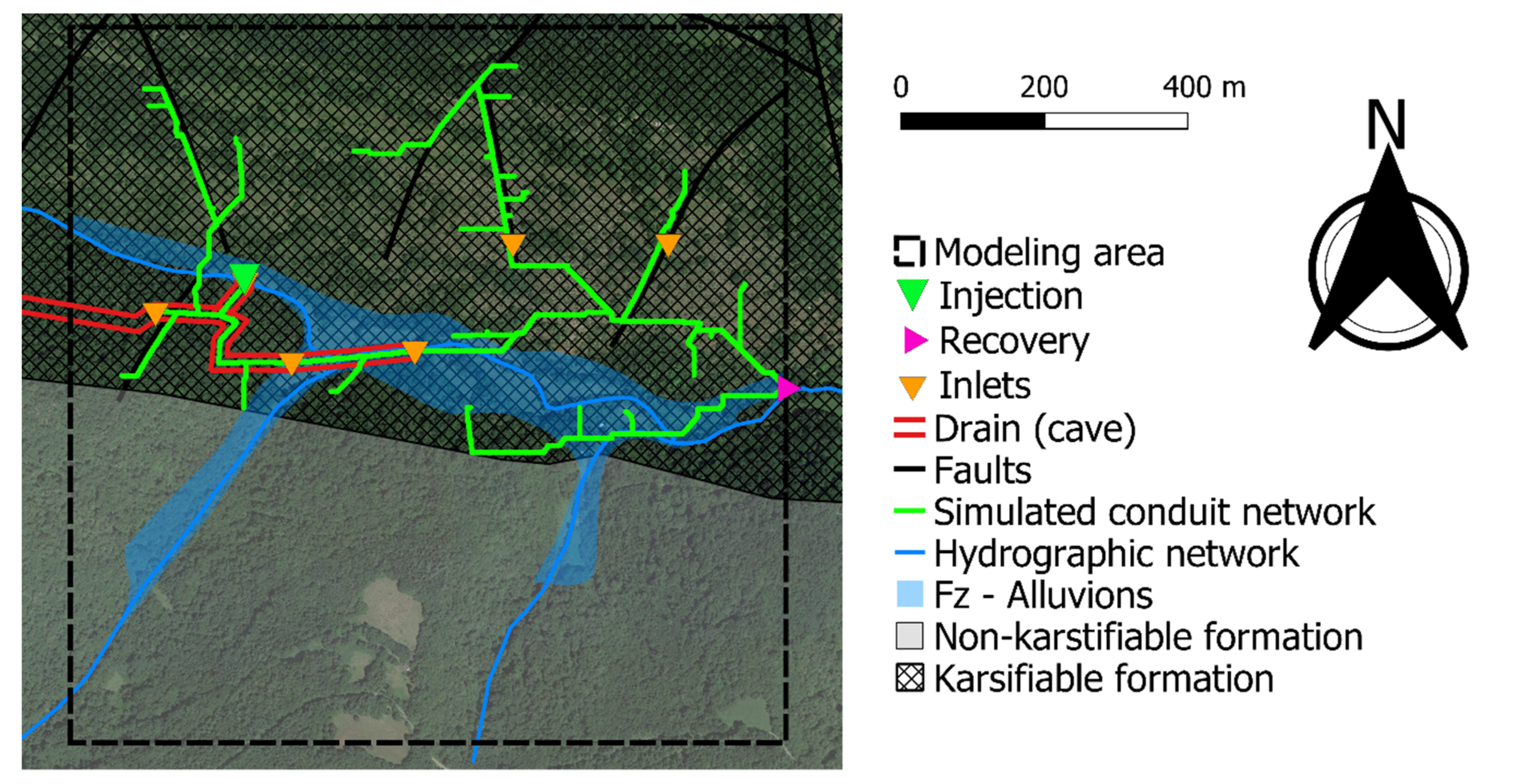
An example of a simulated conduit network is shown in Figure 4. The modeling area was cut in half between the south part composed of the slaty flysch (non-karstifiable formation) and the north part composed of Jurassic limestone (karstifiable formation). To honor the geological observations over the area, the conduits were not simulated in flysch, since it is considered to be a non-karstifiable formation. Then, the conduits were only simulated in the karstic limestone using SKS, and not in the flysch (non-karstifiable formation). Injection and recovery points were imposed based on the topographic survey. Then, the mean slope of the conduit network is around 1:1000 from West to East, between La Peyrère, where the first channel arrives at 508 m a.s.l. [44] and Las Hountas at 498 m a.s.l. [41]. The inlet constitutes an infiltration point from which the FMA can be computed. For better realism, a random inlet can be added for the FMA computation. Fractures are given as a fast flow structure and so can constitute a preferential path for conduit development. As the simulation area was of small extension, the lithology was considered homogeneous, and no inception horizon has been considered. Also, in this study, the pseudo-genetic approach appears more suitable than the speleogenetic approach as the modeling was calibrated based on short-term information (discharge and fluorescent dye concentration measured over several days) and it was less time-consuming.
The SKS simulation provides the spatial organization of the conduit networks but does not provide the shape and size of the conduits section. Some assumptions are needed for those parameters to run flow and solute transport simulation in SWMM. The simulation provided better results considering a rectangular shape, as in previous studies [34,36]. So, the geometry is described by the height H and width W parameters. To consider some natural heterogeneities, the value for each conduit section was sampled in a uniform law such as H ∈ (1.0, 1.5) m and W ∈ (5.0, 7.0) m. In the same way, the Manning’s roughness coefficient n was sampled in a uniform law such as n ∈ (0.045, 0.055) corresponding to an order of magnitude for irregular and rough channel. For numerical reasons, the injection of fluorescent dye was simulated by considering an injection at a constant concentration over a one-time step. In theory, it corresponded to a Heaviside function rather than a Dirac function. In practice, tracer injection was considered to be a Dirac function, and so injected instantaneously [67]. This hypothesis is still acceptable when the time of injection is sufficiently short compared to the mean time of residence. Moreover, as the modeling approach focuses on solute transport on a short-term scale, the discharge was considered to be a linear division of the measured spring discharge between the different inlets. The discharge was considered not to be influenced by recharge during the tracer test as there was no significant rainfall during the tracer tests and it includes short term discharge variations linked to the emptying of the system.
3.2. Statistical Analysis
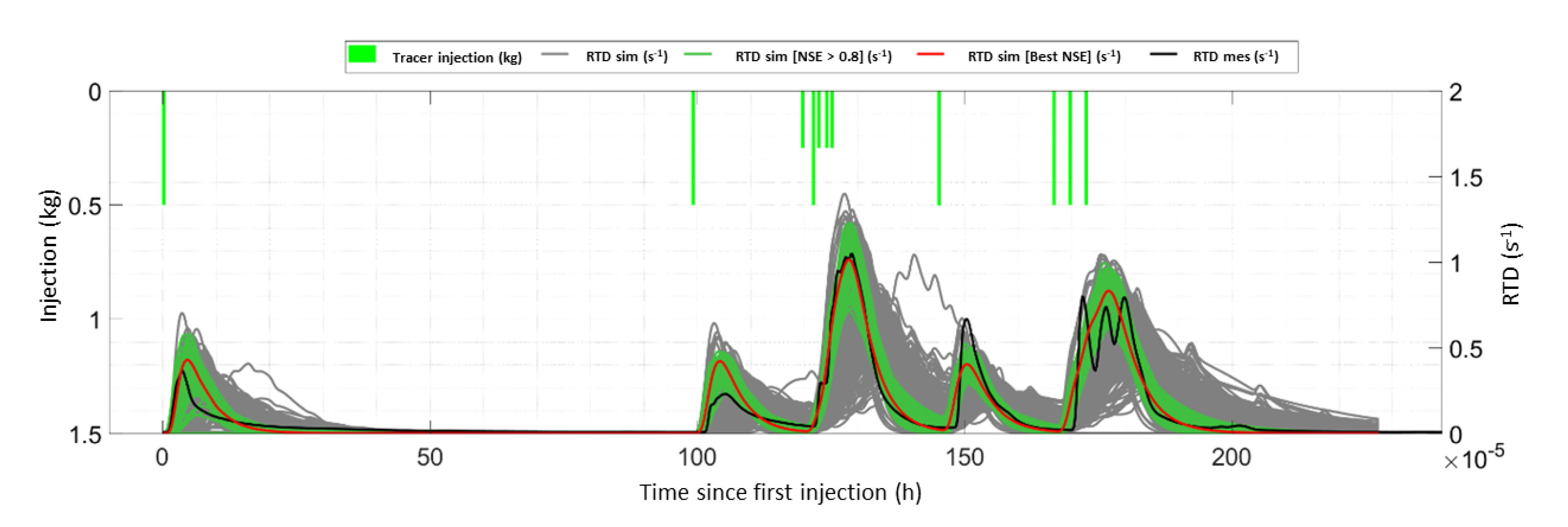
The modeling approach (Figure 3) was performed over 1000 simulations. The simulated RTDs were compared to the observed RTD through the Nash-Sutcliff Efficiency coefficient (NSE) [57] with 174 simulations providing an NSE greater than 0.8 (Figure 5). The shape of the RTD was globally well-reproduced. However, some specific problems can be highlighted. Firstly, the tailing effect appears to be underestimated on the two first tracer-tests recovery. Later in the observed RTD, the tailing effect seems to be less important, so the model gave a quite good fitting despite the curve superposition corresponding to the successive artificial tracer injections. Secondly, the maximum value for 1st (~1 h) 2nd (~100 h) and 4th (~150 h) RTD peaks were poorly simulated. These correspond to lower peak values, in the entire observed RTD. Here, the simulations were selected using the NSE coefficient, which is frequently used in hydrology for multi-peak time series evaluation but tends to favor the high values to the detriment of lower values [68,69]. Moreover, considering the three last injections, the multiple peaked RTD shape was not reproduced. On the opposite, the main recovery, corresponding to the tracer injection 3 to 7 (~120 h after first tracer injection), appeared to be well reproduced. Moreover, some simulations appear to be out of range, with low NSE values (or negative values). The modeling approach proposed here allows investigation of a range of geometry and boundary conditions sufficiently large to investigate their effects on solute transport. Also, the statistical analysis of the results seems to be adequate as there is an acceptable proportion of simulation providing physically acceptable results.
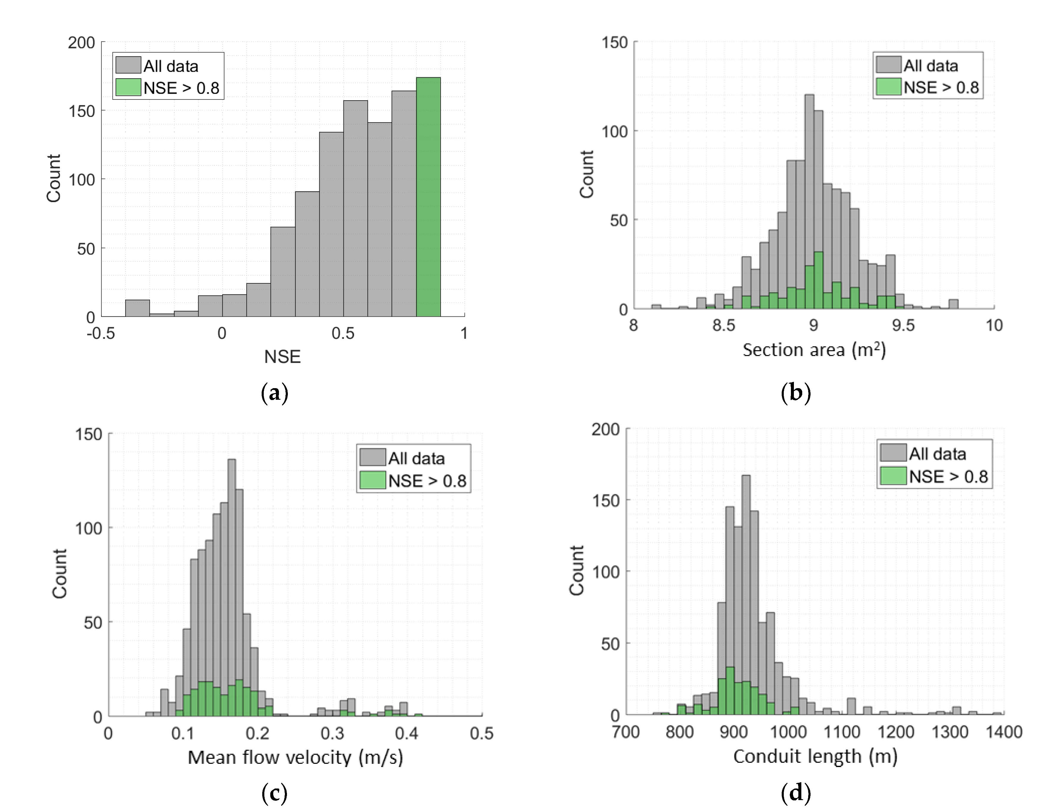
Considering the simulations providing an NSE greater than 0.8 some basic statistics can be calculated (Table 1). The mean flow section along the tracer transport is about 9 m2, the mean flow velocity is 0.16 m/s and the mean length of the conduits between injection and recovery point was about 905 m. Dividing the length of the total conduits by the apparent distance between injection and recovery point gives and estimation of tortuosity. In karst systems, the tortuosity generally varies from 1.10 to 1.40 depending on the morphology of the conduit networks [70]. Considering an apparent distance of 850 m between injection and recovery sites [13], the mean tortuosity here is about 1.06, getting closer to the range of value for an angular maze conduit network morphology [70]. The variability of the mean flow section along the transport and the length of transport appears to be lower than for the mean flow velocity. Moreover, both present a unimodal distribution contrary to the mean flow velocity showing 3 modes (Figure 6). Nonetheless, the two modes showing higher flow velocity values count a low number of simulations in contrast with the mode showing values from 0.1 to 0.2 m/s. The mean flow velocity is considered both in temporal (during tracer recovery) and spatial (along with the entire tracer transport) terms. Considering spatial variations of the conduit section along with the tracer transport pathway may lead to significant variations in flow velocity.
3.3. Conduit Geometry and Spatial Distribution of Flow
The above-mentioned results highlight the ability of the proposed workflow to provide some physically realistic results in terms of RTD shapes and of mean flow section, mean flow velocity and conduit length, which are the basic variable for application of an ADE approach.
In this study, the modeling focused on solving the inverse problem from artificial tracer tests. The entire conduit networks have been simulated to provide numbers of synthetic models in agreement with field observation (geology and heterogeneities such as faults and fractures) and with realistic features such as inputs from a secondary branch. The latter can play an important role in spatial heterogeneities of flow and transport.
In the same way, the simulations with NSE greater than 0.8 were considered for the analysis. The upstream part of the simulated conduit networks was strongly constrained by conditional data, and shows a low range of shapes for the simulated tracer pathway. On the opposite, the downstream part is characterized by a larger range of tracer paths (Figure 7). Considering the principal orientation of the conduit networks in the West to East direction, the transport of the tracer takes place in a 200 m wide corridor in the North-South axis. In addition, this corridor appears to be thinner in the upstream part of the area.
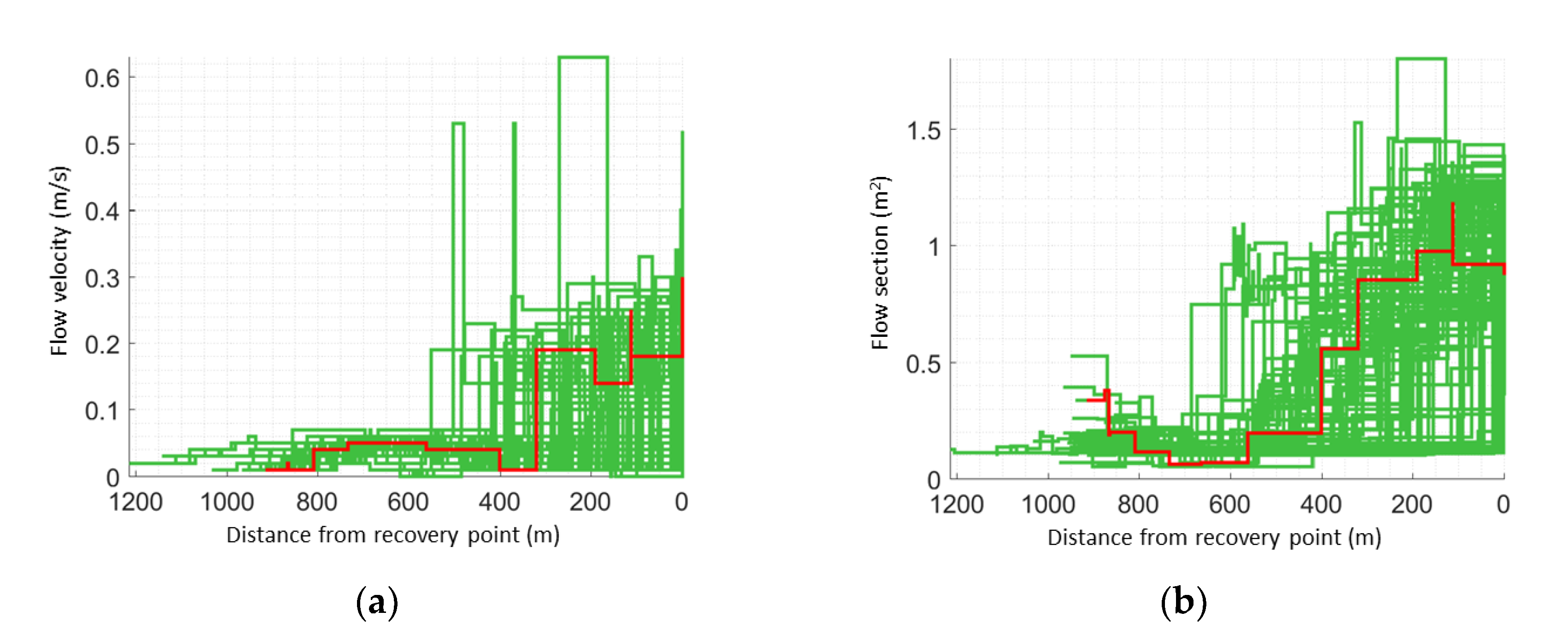
Both the flow velocity and flow section are extracted for each part of the conduit networks along with the tracer transport. The flow velocity and the flow section can be presented as a function of the distance from the outlet (Figure 8). Both presented a significative variability along with the tracer transport. The flow velocity increased around 400 to 500 m from the outlet. This was the consequence of a secondary feeding branch in the conduit networks. In a quite similar way, the flow section increased in the second part of the tracer transport. Moreover, these two parameters show significative variations on a short spatial scale because of the complex structure of karstic aquifers. The shape and size of the conduits present naturally a range of variability. This point has been taken into consideration to provide better realism in the flow and transport simulation.
4. Discussion and Conclusions
The modeling workflow proposed in this study allowed us to simulate artificial tracer tests in synthetic karst systems with imposed boundary conditions. The simulated data were compared to artificial tracer tests performed over the Baget karstic watershed.
The main objective of the study was to assess whether one can characterize karst conduit network geometry from artificial tracer tests. The conduit network modeling includes field observations (geology, heterogeneities such as fault or fractures and speleological information) and was tested against RTD curves derived from artificial tracer tests. The upstream part of the modeling area was constrained by the speleological investigations [44] and therefore most of the simulated conduit network geometries show little variability. So, most of the simulation presented a quite similar structure in the area where there are conditional data. On the contrary, the main drainage structure in the downstream part of the simulation area was unknown. The inverse procedure based on the artificial tracer test data has generated several different network geometries that reproduce the RTD shape measured at the outlet. Moreover, the proposed approach highlighted that some simulated tracer paths may also honor the artificial tracer test data, even if they don’t honor speleological observations. Water coloration has been observed at Moulo de Jaur during tracer tests, ascertaining the transit of the tracer in this area. So one can assume that the tracer transport occurs here, but since there is no possible mass balance computation at this point (absence of concentration and discharge measurements), it is not possible to say that it concerns the total amount of tracer.
Some complementary field investigations, such as an electrical resistivity tomography (ERT) survey, could allow to better constrain the geometry of the simulated conduits over the area [45]. However, as the ERT measurement may be strongly influenced by the presence of water, the ERT survey performed over the Baget area does not provide sufficient information to be considered as conditioning data in the conduit network simulations. Nonetheless, ERT results interpretation can be used as a posterior validation tool for conduit geometries and more broadly the groundwater flow path. This point may constitute an open question for further investigations about hydrogeophysics since recent studies highlighted successfully applied geophysics applications for karst features detection [71,72,73].
Previous studies highlighted that the Baget karstic system response to artificial tracer tests is sensitive to short-term variations in boundary conditions [13]. The flow simulation was performed assuming transient flow conditions with SWMM. By the way, the numerical tracer test simulations consider the perfect mixing assumption in a simulated conduit network subject to several successive injections. For each of these injections, the solute transport was simulated considering temporal variations for flow conditions, even on a short-term scale (infra-hourly scale).
The results provide some interesting perspectives in the use of such an approach for intrinsic aquifer vulnerability mapping. Considering a large number of simulations, it could be possible to build a map of the probability of occurrence of drainage structure over the area. Since the proposed modeling approach provides equiprobability simulations, one can run a K parameter (karst network development) weighing in intrinsic vulnerability mapping methods such as EPIK [74,75,76], depending on the probability for the area to be crossed by a drain.
Finally, the solute transport was simulated on the assumption of perfect and instantaneous mixing. Obtained modeling results could be further improved using an ADE approach. Further work might be performed to implement ADE model computation in the workflow using existing codes such as OTIS [52] or OM-MADE [53]. The reach and the needed parameters (flow velocity, section area) can be directly derived from the SWMM simulations.
Author Contributions
Conceptualization, V.S.; methodology, V.S.; software, P.R. and V.S.; validation, V.S., P.R., and D.L.; formal analysis, V.S.; investigation, V.S.; resources, D.L.; data curation, V.S.; writing—original draft preparation, V.S.; writing—review and editing, V.S., P.R., and D.L.; visualization, V.S.; supervision, D.L.; project administration, D.L.; funding acquisition, D.L., and V.S. All authors have read and agreed to the published version of the manuscript.
Funding
This research has been partially funded by the European and International Relations Department at the University of Toulouse through an International Mobility Assistance.
Acknowledgments
The authors would like to thank the KARST observatory network (SNO KARST) initiative at the INSU/CNRS, which aims to strengthen knowledge sharing and promote cross-disciplinary research on karst systems at the national scale. The authors would like to thank Franck Brehier for the discussion about speleological investigations over the Baget area and Zacharie Alabraeil for his help on performing artificial tracer tests. Also, the authors show their gratitude to Cécile Vuilleumier and Chloé Fandel for their precious help at the beginning of the modeling project.
Conflicts of Interest
The authors declare no conflict of interest.
References
- Király, L. Rapport sur l’état actuel des connaissances dans le domaine des caractères physiques des roches karstiques. Hydrogeol. Karstic Terrains (Hydrogéol. Des Terrains Karstiques) Int. Union Geol. Sci. 1975, 3, 53–67. [Google Scholar]
- Palmer, A.N. Origin and morphology of limestone cave. Geol. Soc. Am. Bull. 1991, 103, 1–21. [Google Scholar] [CrossRef]
- Borghi, A.; Renard, P.; Cornaton, F. Can one identify karst conduit networks geometry and properties from hydraulic and tracer test data? Adv. Water Resour. 2016, 90, 99–115. [Google Scholar] [CrossRef] [Green Version]
- Ford, D.; Williams, P.D. Karst Hydrogeology and Geomorphology; John Wiley & Sons, Inc.: Hoboken, NJ, USA, 2007; ISBN 978-0-470-84996-5. [Google Scholar]
- Chalikakis, K.; Plagnes, V.; Guerin, R.; Valois, R.; Bosch, F.P. Contribution of geophysical methods to karst-system exploration: An overview. Hydrogeol. J. 2011, 19, 1169–1180. [Google Scholar] [CrossRef]
- Field, M.S.; Pinsky, P.F. A two-region nonequilibrium model for solute transport in solution conduits in karstic aquifers. J. Contam. Hydrol. 2000, 44, 329–351. [Google Scholar] [CrossRef]
- Birk, S.; Geyer, T.; Liedl, R.; Sauter, M. Process-based interpretation of tracer tests in carbonate aquifers. Ground Water 2005, 43, 381–388. [Google Scholar] [CrossRef]
- Massei, N.; Wang, H.Q.; Field, M.S.; Dupont, J.P.; Bakalowicz, M.; Rodet, J. Interpreting tracer breakthrough tailing in a conduit-dominated karstic aquifer. Hydrogeol. J. 2006, 14, 849–858. [Google Scholar] [CrossRef]
- Goldscheider, N. A new quantitative interpretation of the long-tail and plateau-like breakthrough curves from tracer tests in the artesian karst aquifer of Stuttgart, Germany. Hydrogeol. J. 2008, 16, 1311–1317. [Google Scholar] [CrossRef] [Green Version]
- Labat, D.; Mangin, A. Transfer function approach for artificial tracer test interpretation in karstic systems. J. Hydrol. 2015, 529, 866–871. [Google Scholar] [CrossRef]
- Duran, L.; Fournier, M.; Massei, N.; Dupont, J.-P. Assessing the Nonlinearity of Karst Response Function under Variable Boundary Conditions. Ground Water 2016, 54, 46–54. [Google Scholar] [CrossRef]
- Ender, A.; Goeppert, N.; Goldscheider, N. Spatial resolution of transport parameters in a subtropical karst conduit system during dry and wet seasons. Hydrogeol. J. 2018, 26, 2241–2255. [Google Scholar] [CrossRef]
- Sivelle, V.; Labat, D. Short-term variations in tracer-test responses in a highly karstified watershed. Hydrogeol. J. 2019, 27, 2061–2075. [Google Scholar] [CrossRef]
- Morales, T.; Uriarte, J.A.; Olazar, M.; Antigüedad, I.; Angulo, B. Solute transport modelling in karst conduits with slow zones during different hydrologic conditions. J. Hydrol. 2010, 390, 182–189. [Google Scholar] [CrossRef]
- Dewaide, L.; Collon, P.; Poulain, A.; Rochez, G.; Hallet, V. Double-peaked breakthrough curves as a consequence of solute transport through underground lakes: A case study of the Furfooz karst system, Belgium. Hydrogeol. J. 2018, 26, 641–650. [Google Scholar] [CrossRef]
- Field, M.S.; Leij, F.J. Solute transport in solution conduits exhibiting multi-peaked breakthrough curves. J. Hydrol. 2012, 440–441, 26–35. [Google Scholar] [CrossRef]
- Vincenzi, V.; Riva, A.; Rossetti, S. Towards a better knowledge of Cansiglio karst system (Italy): Results of the first successful groundwater tracer test. Acta Carsologica 2011, 40. [Google Scholar] [CrossRef] [Green Version]
- Filippini, M.; Squarzoni, G.; De Waele, J.; Fiorucci, A.; Vigna, B.; Grillo, B.; Riva, A.; Rossetti, S.; Zini, L.; Casagrande, G.; et al. Differentiated spring behavior under changing hydrological conditions in an alpine karst aquifer. J. Hydrol. 2018, 556, 572–584. [Google Scholar] [CrossRef]
- Hauns, M.; Jeannin, P.-Y.; Atteia, O. Dispersion, retardation and scale effect in tracer breaktrough curves in karst conduits. J. Hydrol. 2001, 241, 177–193. [Google Scholar] [CrossRef]
- Mohammadi, Z.; Gharaat, M.J.; Field, M. The Effect of Hydraulic Gradient and Pattern of Conduit Systems on Tracing Tests: Bench-Scale Modeling. Groundwater 2018, 57, 110–125. [Google Scholar] [CrossRef] [Green Version]
- Zhao, X.; Chang, Y.; Wu, J.; Xue, X. Effects of flow rate variation on solute transport in a karst conduit with a pool. Environ. Earth Sci. 2019, 78, 237. [Google Scholar] [CrossRef]
- Thrailkill, J. Pipe Flow Models of a Kentucky Limestone Aquifer. Groundwater 1974, 12, 202–205. [Google Scholar] [CrossRef]
- Jeannin, P.-Y. Modeling flow in phreatic and epiphreatic karst conduits in the Hölloch cave (Muotatal, Switzerland). Water Resour. Res. 2001, 37, 191–200. [Google Scholar] [CrossRef]
- Gill, L.W.; Naughton, O.; Johnston, P.M. Modeling a network of turloughs in lowland karst. Water Resour. Res. 2013, 49, 3487–3503. [Google Scholar] [CrossRef]
- Schuler, P.; Duran, L.; McCormack, T.; Gill, L. Submarine and intertidal groundwater discharge through a complex multi-level karst conduit aquifer. Hydrogeol. J. 2018, 26, 2629–2647. [Google Scholar] [CrossRef] [Green Version]
- Shoemaker, W.B.; Kuniansky, E.L.; Birk, S.; Bauer, S.; Swain, E.D. Documentation of a Conduit Flow Process (CFP) for MODFLOW-2005; U.S. Geological Survey: Reston, VA, USA, 2008. [Google Scholar]
- Barenblatt, G.I.; Zheltov, I.P.; Kochina, I.N. Basic concepts in the theory of seepage of homogeneous liquids in fissured rocks. J. Appl. Math. Mech. 1960, 24, 1286–1303. [Google Scholar] [CrossRef]
- Chang, Y.; Wu, J.; Jiang, G.; Liu, L.; Reimann, T.; Sauter, M. Modelling spring discharge and solute transport in conduits by coupling CFPv2 to an epikarst reservoir for a karst aquifer. J. Hydrol. 2019, 569, 587–599. [Google Scholar] [CrossRef]
- Xu, Z.; Hu, B.X.; Davis, H.; Cao, J. Simulating long term nitrate-N contamination processes in the Woodville Karst Plain using CFPv2 with UMT3D. J. Hydrol. 2015, 524, 72–88. [Google Scholar] [CrossRef]
- Xu, Z.; Hu, B.X.; Davis, H.; Kish, S. Numerical study of groundwater flow cycling controlled by seawater/freshwater interaction in a coastal karst aquifer through conduit network using CFPv2. J. Contam. Hydrol. 2015, 182, 131–145. [Google Scholar] [CrossRef] [Green Version]
- Xu, Z.; Hu, B.X. Development of a discrete-continuum VDFST-CFP numerical model for simulating seawater intrusion to a coastal karst aquifer with a conduit system. Water Resour. Res. 2017, 53, 688–711. [Google Scholar] [CrossRef]
- Assari, A.; Mohammadi, Z. Assessing flow paths in a karst aquifer based on multiple dye tracing tests using stochastic simulation and the MODFLOW-CFP code. Hydrogeol. J. 2017, 25, 1679–1702. [Google Scholar] [CrossRef]
- Gironás, J.; Roesner, L.A.; Rossman, L.A.; Davis, J. A new applications manual for the Storm Water Management Model (SWMM). Environ. Model. Softw. 2010, 25, 813–814. [Google Scholar] [CrossRef]
- Peterson, E.W.; Wicks, C.M. Assessing the importance of conduit geometry and physical parameters in karst systems using the storm water management model (SWMM). J. Hydrol. 2006, 329, 294–305. [Google Scholar] [CrossRef]
- Wu, Y.; Jiang, Y.; Yuan, D.; Li, L. Modeling hydrological responses of karst spring to storm events: Example of the Shuifang spring (Jinfo Mt., Chongqing, China). Environ. Geol. 2008, 55, 1545–1553. [Google Scholar] [CrossRef]
- Vuilleumier, C. Hydraulics and Sedimentary Processes in the Karst Aquifer of Milandre (Jura Mountains, Switzerland). Ph.D. Thesis, Université de Neuchâtel, Neuchâtel, Switzerland, 2017. [Google Scholar]
- Borghi, A.; Renard, P.; Jenni, S. A pseudo-genetic stochastic model to generate karstic networks. J. Hydrol. 2012, 414–415, 515–529. [Google Scholar] [CrossRef]
- Jourde, H.; Massei, N.; Mazzilli, N.; Binet, S.; Batiot-Guilhe, C.; Labat, D.; Steinmann, M.; Bailly-Comte, V.; Seidel, J.L.; Arfib, B.; et al. SNO KARST: A French Network of Observatories for the Multidisciplinary Study of Critical Zone Processes in Karst Watersheds and Aquifers. Vadose Zone J. 2018, 17, 1–18. [Google Scholar] [CrossRef] [Green Version]
- Choukroune, P. Tectonic evolution of the Pyrenees. Annu. Rev. Earth Planet. Sci. 1992, 20, 143–158. [Google Scholar] [CrossRef]
- Angrand, P. Évolution 3D D’un Rétro-Bassin D’avant-Pays: Le Bassin Aquitain, France. Ph.D. Thesis, Université de Lorraine, Lorraine, France, 2017. [Google Scholar]
- Mangin, A. Contribution à L’étude Hydrodynamique des Aquifères Karstiques. Ph.D. Thesis, Université de Dijon, Dijon, France, 1975. [Google Scholar]
- Johnson, J.A.; Hall, C.A. The structural and sedimentary evolution of the Cretaceous North Pyrenean Basin, southern France. Geol. Soc. Am. Bull. 1989, 101, 231–247. [Google Scholar] [CrossRef]
- Genthon, P.; Bataille, A.; Fromant, A.; D’Hulst, D.; Bourges, F. Temperature as a marker for karstic waters hydrodynamics. Inferences from 1 year recording at La Peyrére cave (Ariège, France). J. Hydrol. 2005, 311, 157–171. [Google Scholar] [CrossRef]
- Brehier, F.; Horizon VerticalSaint Girons, France. Speleoglogic Investigations over the Baget Area. Personal Communication, 2019. [Google Scholar]
- Sivelle, V. Couplage D’approches Conceptuelles, Systémiques et Distribuées Pour L’interprétation de Traçages Artificiels en Domaine Karstiques. Implications Pour la Détermination de la Structure Interne des Aquifères Karstiques. Ph.D. Thesis, Université Paul Sabatier-Toulouse III, Touloue, France, 2019. [Google Scholar]
- Rousset, D.; Genthon, P.; Perroud, H.; Sénéchal, G. Detection and Characterization of Near Surface Small Karstic Cavities Using Integrated Geophysical Surveys; European Association of Geoscientists & Engineers: DB Houten, The Netherland, 1998. [Google Scholar]
- Bakalowicz, M.; Crochet, P.; D’Hulst, D.; Mangin, A.; Marsaud, B.; Ricard, J.; Rouch, R. High discharge pumping in a vertical cave, fundamental and applied results. Basic Appl. Hydrogeol. Res. Fr. Karstic Areas 1994, 65, 93–110. [Google Scholar]
- Schnegg, P.-A. An Inexpensive Field Fluorometer for Hydrogeological Tracer Tests with Three Tracers and Turbidity Measurement. Available online: https://doc.rero.ch/record/5068 (accessed on 15 April 2020).
- Sivelle, V.; Labat, D.; Duran, L.; Fournier, M.; Massei, N. Artificial Tracer Tests Interpretation Using Transfer Function Approach to Study the Norville Karst System. In Proceedings of the Eurokarst 2018, Besançon, France, 2–6 July 2018; Bertrand, C., Denimal, S., Steinmann, M., Renard, P., Eds.; Springer International Publishing: Heidelberg, Gemany, 2020; pp. 193–198. [Google Scholar]
- Wang, H.Q.; Crampon, N.; Huberson, S.; Garnier, J.M. A linear graphical method for determining hydrodispersive characteristics in tracer experiments with instantaneous injection. J. Hydrol. 1987, 95, 143–154. [Google Scholar] [CrossRef]
- Lauber, U.; Ufrecht, W.; Goldscheider, N. Spatially resolved information on karst conduit flow from in-cave dye tracing. Hydrol. Earth Syst. Sci. 2014, 18, 435–445. [Google Scholar] [CrossRef] [Green Version]
- Runkel, R.L. One-Dimensional Transport with Inflow and Storage (OTIS): A Solute Transport Model for Streams and Rivers; Water-Resources Investigations Report; Geological Survey (U.S.): Reston, VA, USA, 1998. [Google Scholar]
- Tinet, A.-J.; Collon, P.; Philippe, C.; Dewaide, L.; Hallet, V. OM-MADE: An open-source program to simulate one-dimensional solute transport in multiple exchanging conduits and storage zones. Comput. Geosci. 2019, 127, 23–35. [Google Scholar] [CrossRef]
- BRGM Geological Map at 1:50 000 (Bd-Charm-50), Department: Ariège (09, France). Available online: http://infoterre.brgm.fr/formulaire/telechargement-cartes-geologiques-departementales-150-000-bd-charm-50 (accessed on 30 December 2019).
- IGN BD ALTI® 25M—Orne. Available online: https://geo.data.gouv.fr/fr/datasets/22355590527b92116abf42a509b6defdbf4c0e33 (accessed on 5 April 2020).
- Nash, J.E.; Sutcliffe, J.V. River flow forecasting through conceptual models part I—A discussion of principles. J. Hydrol. 1970, 10, 282–290. [Google Scholar] [CrossRef]
- Debroas, E.-J. Géologie du bassin versant du Baget (Zone nord-pyrénéenne, Ariège, France): Nouvelles observations et conséquences. Strata 2009, 2, 1–93. [Google Scholar]
- Sisavath, S.; Mourzenko, V.; Genthon, P.; Thovert, J.-F.; Adler, P.M. Geometry, percolation and transport properties of fracture networks derived from line data. Geophys. J. Int. 2004, 157, 917–934. [Google Scholar] [CrossRef] [Green Version]
- Debroas, E.J. Modele de bassin triangulaire a l’intersection de decrochements divergents pour le fosse albo-cenomanien de la Ballongue (zone nord-pyreneenne, France). Bull. Soc. Géol. Fr. 1987, 3, 887–898. [Google Scholar] [CrossRef]
- Sethian, J.A. A fast marching level set method for monotonically advancing fronts. Proc. Natl. Acad. Sci. USA 1996, 93, 1591–1595. [Google Scholar] [CrossRef] [Green Version]
- Aryo, D. Dijkstra Algorithm. Available online: https://www.mathworks.com/matlabcentral/fileexchange/36140 (accessed on 21 June 2019).
- Sivelle, V.; Labat, D.; Mazzilli, N.; Massei, N.; Jourde, H. Dynamics of the Flow Exchanges between Matrix and Conduits in Karstified Watersheds at Multiple Temporal Scales. Water 2019, 11, 569. [Google Scholar] [CrossRef] [Green Version]
- Worthington, S.R.H.; Soley, R.W.N. Identifying turbulent flow in carbonate aquifers. J. Hydrol. 2017, 552, 70–80. [Google Scholar] [CrossRef]
- De Saint-Venant, A.; Barré, D.; Saint-Cyr, J. Théorie du Mouvement Non-Permanent des Eaux, Avec Application Aux Crues des Rivières et à L’introduction des Marées Dans Leur Lit; Académie des Sciences: Paris, France, 1871. [Google Scholar]
- Rossman, L.A. Storm Water Management Model User’s Manual, Version 5.0; National Risk Management Research Laboratory, Office of Research and Development, US Environmental Protection Agency: Cincinnati, OH, USA, 2010. [Google Scholar]
- Metcalf, E. Storm Water Management Model, Volume I-Final Report; University of Florida and Water Resources Engineers, Inc.: Washington, DC, USA, 1971. [Google Scholar]
- Goldscheider, N.; Meiman, J.; Pronk, M.; Smart, C. Tracer tests in karst hydrogeology and speleology. Int. J. Speleol. 2008, 37, 27–40. [Google Scholar] [CrossRef] [Green Version]
- Gupta, H.V.; Kling, H.; Yilmaz, K.K.; Martinez, G.F. Decomposition of the mean squared error and NSE performance criteria: Implications for improving hydrological modelling. J. Hydrol. 2009, 377, 80–91. [Google Scholar] [CrossRef] [Green Version]
- Pool, S.; Vis, M.; Seibert, J. Evaluating model performance: Towards a non-parametric variant of the Kling-Gupta efficiency. Hydrol. Sci. J. 2018, 63, 1941–1953. [Google Scholar] [CrossRef]
- Jouves, J.; Viseur, S.; Arfib, B.; Baudement, C.; Camus, H.; Collon, P.; Guglielmi, Y. Speleogenesis, geometry, and topology of caves: A quantitative study of 3D karst conduits. Geomorphology 2017, 298, 86–106. [Google Scholar] [CrossRef] [Green Version]
- Xu, S.; Sirieix, C.; Riss, J.; Malaurent, P. A clustering approach applied to time-lapse ERT interpretation—Case study of Lascaux cave. J. Appl. Geophys. 2017, 144, 115–124. [Google Scholar] [CrossRef]
- Cheng, Q.; Chen, X.; Tao, M.; Binley, A. Characterization of karst structures using quasi-3D electrical resistivity tomography. Environ. Earth Sci. 2019, 78, 285. [Google Scholar] [CrossRef] [Green Version]
- Bermejo, L.; Ortega, A.I.; Guérin, R.; Benito-Calvo, A.; Pérez-González, A.; Parés, J.M.; Aracil, E.; de Bermúdez Castro, J.M.; Carbonell, E. 2D and 3D ERT imaging for identifying karst morphologies in the archaeological sites of Gran Dolina and Galería Complex (Sierra de Atapuerca, Burgos, Spain). Quat. Int. 2017, 433, 393–401. [Google Scholar] [CrossRef]
- Doerfliger, N.; Jeannin, P.-Y.; Zwahlen, F. Water vulnerability assessment in karst environments: A new method of defining protection areas using a multi-attribute approach and GIS tools (EPIK method). Environ. Geol. 1999, 39, 165–176. [Google Scholar] [CrossRef] [Green Version]
- Doerfliger, N.; Zwahlen, F. Practical Guide: Groundwater Vulnerability Mapping in Karstic Regions (EPIK); Agency for the Environment, Forests and Landscape (SAEFL): Bern, Switzerland, 1998; Volume 56. [Google Scholar]
- Ollivier, C.; Lecomte, Y.; Chalikakis, K.; Mazzilli, N.; Danquigny, C.; Emblanch, C. A QGIS Plugin Based on the PaPRIKa Method for Karst Aquifer Vulnerability Mapping. Groundwater 2019, 57, 201–204. [Google Scholar] [CrossRef]
Figure 1.
Location of the Baget karstic system, a geological map of the area (modified from [54]) and limits of the watershed (red dashed line). The study area concerns the downstream part of the watershed (black dashed line), in the mid mountains Lachein valley, characterized by altitude from 450 m a.s.l. to 750 m a.s.l. [55]. The pictures show remarkable features across the area: (A) La Peyrère is a cave connected to the main drainage system, (B) P2 Loss is the point of injection for artificial tracer tests, (C) La Hillère is a temporary resurgence, (D) Moulo de Jaur is a temporary resurgence and an intermediate observation point of tracer transport, (E) Las Hountas is the perennial spring of the watershed and the tracer recovery point and (F) B1 is the gauging station (discharge, water sampling, and fluorimeter), modified from [13].

Figure 2.
Rainfall-discharge time series during artificial tracer tests and injection recovery time series. The artificial tracer tests have been performed in April 2018 (modified from [13]).
Figure 2.
Rainfall-discharge time series during artificial tracer tests and injection recovery time series. The artificial tracer tests have been performed in April 2018 (modified from [13]).

Figure 3.
Coupling the Stochastic Karst Simulator (SKS) and Storm Water Management Model (SWMM) to solve the inverse problem based on artificial tracer tests. SKS is used to simulate the conduit network geometry and SWMM is used to simulate flow and solute transport, assuming an instantaneous complete mixing hypothesis.

Figure 4.
Simulation of a karst conduit network over the downstream part of the Baget watershed using the SKS algorithm.
Figure 4.
Simulation of a karst conduit network over the downstream part of the Baget watershed using the SKS algorithm.

Figure 5.
Tracer injection (green bars), experimental residence time distribution (RTD; black solid line) and simulated RTD curves: grey lines represent simulated RTD for all scenarios, green lines represent simulated RTD with an Nash-Sutcliff Efficiency coefficient (NSE) superior to 0.8 and the red line is the simulation providing the best NSE (0.89).

Figure 6.
Histograms calculated over 1000 simulations on (a) NSE coefficient, (b) section area, (c) the mean flow velocity and (d) the conduit length. Grey bars are for all data and green bars represent the simulations providing an NSE superior to 0.8 between simulated RTD and observed RTD.
Figure 6.
Histograms calculated over 1000 simulations on (a) NSE coefficient, (b) section area, (c) the mean flow velocity and (d) the conduit length. Grey bars are for all data and green bars represent the simulations providing an NSE superior to 0.8 between simulated RTD and observed RTD.

Figure 7.
2D representation of the simulated tracer pathways, extracted from the synthetic conduit networks simulated with SKS.
Figure 7.
2D representation of the simulated tracer pathways, extracted from the synthetic conduit networks simulated with SKS.

Figure 8.
(a) Flow velocity along with the tracer transport and (b) flow section along with the tracer transport. Green lines correspond to simulations providing an NSE superior to 0.8 and red lines correspond to simulation providing the best NSE (0.89).
Figure 8.
(a) Flow velocity along with the tracer transport and (b) flow section along with the tracer transport. Green lines correspond to simulations providing an NSE superior to 0.8 and red lines correspond to simulation providing the best NSE (0.89).


Table 1.
Statistics based the simulation with an NSE > 0.8 (174 simulations).
| Descriptive Statistics | Mean Flow Section Area (m2) | Mean Flow Velocity (m/s) | Transport Length (m) |
|---|---|---|---|
| Min | 8.42 | 0.09 | 772.7 |
| Max | 9.45 | 0.41 | 1007.0 |
| Mean | 9.01 | 0.16 | 905.5 |
| Standard Deviation | 0.20 | 0.06 | 43.1 |
| Variation Coefficient | 0.02 | 0.14 | 0.05 |
© 2020 by the authors. Licensee MDPI, Basel, Switzerland. This article is an open access article distributed under the terms and conditions of the Creative Commons Attribution (CC BY) license (http://creativecommons.org/licenses/by/4.0/).
Share and Cite
MDPI and ACS Style
Sivelle, V.; Renard, P.; Labat, D. Coupling SKS and SWMM to Solve the Inverse Problem Based on Artificial Tracer Tests in Karstic Aquifers. Water 2020, 12, 1139. https://doi.org/10.3390/w12041139
AMA Style
Sivelle V, Renard P, Labat D. Coupling SKS and SWMM to Solve the Inverse Problem Based on Artificial Tracer Tests in Karstic Aquifers. Water. 2020; 12(4):1139. https://doi.org/10.3390/w12041139
Chicago/Turabian StyleSivelle, Vianney, Philippe Renard, and David Labat. 2020. "Coupling SKS and SWMM to Solve the Inverse Problem Based on Artificial Tracer Tests in Karstic Aquifers" Water 12, no. 4: 1139. https://doi.org/10.3390/w12041139
Note that from the first issue of 2016, this journal uses article numbers instead of page numbers. See further details here.