Removing Wave Bias from Velocity Measurements for Tracer Transport: The Harmonic Analysis Approach
by
 , ,
, ,
Sangdon So
1,*, 
Arnoldo Valle-Levinson
1,
Jorge Armando Laurel-Castillo
2,
Junyong Ahn
3 and
Mohammad Al-Khaldi
4 1
Civil and Coastal Engineering, University of Florida, Gainesville, FL 32611, USA
2
National Water Commission, Mexico City 04340, Mexico
3
Mechanical and Civil Engineering, Florida Institute of Technology, Melbourne, FL 32901, USA
4
Kuwait Institute for Scientific Research, Safat 13109, Kuwait
*
Author to whom correspondence should be addressed.
Water 2020, 12(4), 1138; https://doi.org/10.3390/w12041138
Submission received: 4 September 2019
/
Revised: 13 April 2020
/
Accepted: 13 April 2020
/
Published: 16 April 2020
(This article belongs to the Special Issue Tracer and Timescale Methods for Passive and Reactive Transport in Fluid Flows)
Abstract
:Estimates of turbulence properties with Acoustic Doppler Current Profiler (ADCP) measurements can be muddled by the influence of wave orbital velocities. Previous methods—Variance Fit, Vertical Adaptive Filtering (VAF), and Cospectra Fit (CF)—have tried to eliminate wave-induced contamination. However, those methods may not perform well in relatively energetic surface gravity wave or internal wave conditions. The Harmonic Analysis (HA) method proposed here uses power spectral density to identify waves and least squares fits to reconstruct the identified wave signals in current velocity measurements. Then, those reconstructed wave signals are eliminated from the original measurements. Datasets from the northeastern Gulf of Mexico and Cape Canaveral, Florida, are used to test this approach and compare it with the VAF method. Reynolds stress estimates from the HA method agree with the VAF method in the lower half of the water column because wave energy decays with depth. The HA method performs better than the VAF method near the surface during pulses of increased surface gravity wave energy.
1. Introduction
The range of fluid and tracer dynamics in aquatic systems extends from basin scale, up to approximately 10,000 km in the ocean, to turbulence scale, approximately 1 mm, which is related to the dissipation of Turbulent Kinetic Energy (m2/s3 or Watt/kg) [1,2,3]. Turbulent Kinetic Energy has a critical effect in transporting and changing the local concentration of ocean tracers such as dissolved oxygen, carbon dioxide, nutrients, plankton, and pollutants. Processes at the air–water interface can influence the transport and transformation of tracers in the water column. For instance, wind-driven waves can affect tracer concentration and distribution through advection and diffusion. In particular, diffusive processes should be dominated by turbulence, which may be biased by waves because of their overlap in frequency and scale. Thus, the study of diffusion and turbulence in the water column, and its identification from waves’ influence, should allow an understanding of vertical exchange processes that determine the fate of tracers in aquatic environments. It follows that estimating Turbulent Kinetic Energy, including its transport, production, and dissipation, is obscured by the presence of surface waves because, as mentioned above, waves and turbulence share spectral energy bands. A reliable approach for velocity measurements is needed to distinguish the signal related to waves and to turbulence.
Most fluid motions in nature and engineering are turbulent [4]. Measurements of turbulence in the coastal environment can bolster our understanding of vertical exchange of momentum, energy, heat, and any tracer (e.g., nutrients), and they can help us parameterize turbulence in boundary layers [5,6,7,8]. Microstructure measurements have been used to estimate turbulence in the marine environment with devices that either fall, rise, or move horizontally (on an AUV). However, these microstructure measurements are labor intensive and require a dedicated platform [9,10]. Although this approach can produce reliable results, it is logistically and financially unfeasible to collect continuous long-term spatial—in the water column—series of turbulence [11]. The use of anchored shipboard or bottom-mounted Acoustic Doppler Current Profilers (ADCPs) has allowed measurements of time series of turbulent parameters in the water column [9,12,13].
Estimates of tracer transport under turbulent conditions in shallow coastal regions throughout the world may be contaminated by wave action. Turbulence properties may be confused by velocity fluctuations that include orbital velocities generated by multi-scale and multi-directional waves. Unless the effects of wave orbital velocities are eliminated from turbulence assessments, descriptions of tracer transport will be overestimated by at least one order of magnitude. Therefore, in studies of tracer transport, it is essential to implement a reliable approach to eliminate, remove, or at least reduce wave bias.
2. Previous Methods for Removing Wave Bias
Direct turbulence measurements can be overwhelmed by wave motion in coastal and ocean environments [14,15,16]. Observational studies have recognized that velocity covariance produced by waves can be one order of magnitude larger even than the covariance generated by an instrument tilt [16,17]. Several methods have been introduced to remove wave contamination from turbulent velocity measurements. The Velocity Differencing method, introduced by Lohrmann et al. (1990), is based on the assumption that the correlation scale of wave-induced velocity is larger than that of the turbulence. Wave contamination can be reduced by contrasting measurements between two velocimeters that are separated by a distance where the turbulent fluctuations are uncorrelated [17]. This differencing method was extended to ADCPs and named the Variance Fit method [13].
The Variance Fit method [13,14] assumes that the wave-induced velocities along ADCP beams are in phase and that velocities at two different vertical positions are scaled by a constant. An adaptive filtering method was introduced by Shaw and Trowbridge (2001) [15] assuming the wave-induced fluctuations are 100% coherent in space. Rosman et al. (2008) [18] applied the adaptive filtering method to ADCP measurements. Vertical Adaptive Filtering (VAF) and Horizontal Adaptive Filtering (HAF) methods relax the assumptions of the Variance Fit method [18]. These adaptive filtering methods assume that the velocities at a position are a linear function of the velocities at another position rather than a constant [18]. Both of these methods reduce wave bias to an acceptable level in relatively “mild” wave climates [16] by differencing velocities measured by two sensors. Gerbi et al. (2008) [19] proposed an alternative approach showing that the cospectra of the Reynolds stress (, where and are fluctuating parts of horizontal and vertical velocity, respectively) are approximately constant at low frequencies and roll off with a −7/3 slope in the inertial subrange [16]. This method was later extended to ADCP observations by Kirincich et al. (2010) [16]. Scannell et al. (2017) [20] introduced a method to remove the wave bias in the Turbulent Kinetic Energy Dissipation Rate (), which is estimated by a modified structure function. From ADCP data at three depths, they demonstrated that the modified structure function is effective in removing wave bias, compared to the standard structure function [10]. However, this method is limited to the estimation of a structure function.
Free fall profilers recording at high frequencies (>100 Hz) have been developed to observe turbulence. However, data collection is labor-intensive and limits observational periods (Williams and Simpson, 2004). While ADCPs were not ideal to measure turbulence in coastal environments because of their coarse sampling frequency, they have been used widely to derive Reynolds stresses and [12,13]. The variance method for extracting Reynolds stresses from ADCP observations has been applied by different researchers [13,16,18]. In the absence of instrument misalignment and waves, the Reynolds stresses can be computed from the difference of beam velocity variance along opposing beams [12,21]:
where is the demeaned along-beam velocity of 4 beams which are positive toward the transducer, and is the angle formed by the beam and the vertical. By comparing with results from Acoustic Doppler Velocimeters (ADVs), the variance method was validated in Souza and Howarth (2005) [22] and Nidzieko et al. (2006) [23]. However, the variance method failed in the presence of surface waves, because their orbital velocities are orders of magnitude larger than turbulent velocities and bias the estimates [16].
In the presence of surface waves, the velocity components can be decomposed as:
where an overbar denotes a temporal mean value, and tilde and prime are orbital velocities and turbulent fluctuations, respectively. Substituting Equation (3) into Equation (2) yields
with the corresponding expression for Equation (1), where and are instrument tilts, which are commonly referred to as pitch and roll, respectively. The derivation of wave-induced bias is illustrated in detail by Rosman et al. (2008) [18] and Trowbridge (1998) [17]. On the right-hand side of Equation (4), the first term is the unbiased Reynolds stress [18], which is the quantity of interest. The second term is the error due to wave stresses. The third term includes errors of the interaction between waves and the instrument misalignment. The fourth term, the turbulence bias , is insignificant if the sensor misalignment is small [17]. For tilts <3°, the proposed is less than 50% of the true Reynolds stress in the absence of waves [18]. The wave-induced errors, and , are one order of magnitude larger than the Reynolds stresses even if the tilt is small. can be removed by rotating the principal axis where waves propagate [17]. To reduce the error to 10% of the Reynolds stress, one must be able to establish the principal axis, which is not feasible [17] in an open coastal area. Therefore, it is essential to remove wave contamination from the beam velocities before applying the variance method.
The bias produced by surface waves can be reduced to an acceptable level by differencing velocities measured by two sensors [17]. In order to be effective, the two sensors must be separated by a distance shorter than the predominant wavelength and longer than the distance at which the turbulent fluctuations are correlated [15,17]. Hereafter, this method is referred to as the Differencing method. An extension of the Differencing method to ADCP measurements [13] consists of vertically differencing beam velocities () at two locations. One of the velocities is scaled by a parameter that accounts for wave attenuation, in accordance with linear wave theory.
where and denote the demeaned beam velocities, and A and B are two different vertical positions with A being farther from the transducer than B. The scaling parameter can be chosen to minimize the difference of wave orbital velocity variance between two levels:
where wave variances and are computed from linear wave theory. Wave height (, frequency (), and wave number () are determined by fitting a model variance vertical profile, , to the observations of velocity variance (Whipple et al., 2006)
where is the vertical coordinate (zero at the water surface and positive upward), and is the angle formed by the beam and the vertical (approximately 20°).
Assuming is the same for opposing beams, the variance of the remainder yields:
If the distance between A and B is chosen to be such that the turbulent fluctuations are uncorrelated, the third terms on the right hand side of Equations (9) and (10) are zero. The application of the variance method of Equation (2) gives:
Therefore, an average value of the Reynolds stress between positions A and B is:
with the corresponding equation along beams 1 and 2.
Under “high wave energy”, the Differencing method in Equations (5) and (6) can fail to reduce the wave bias to an acceptable level due to the differences of amplitude and phase between two locations [15]. To minimize the wave-induced differences in Equations (5) and (6), Shaw and Trowbridge (2001) [15] used linear filtering techniques. Based on the Differencing method with linear filtering, Rosman et al. (2008) [18] developed vertical and horizontal Differencing methods with Adaptive Filtering, which are henceforth referred to as VAF and HAF, respectively. Instead of using the constant parameter , Rosman et al. (2008) [18], and Shaw and Trowbridge (2001) [15] described the wave velocity at as a linear function () of the wave velocity at by assuming that wave-induced velocities are spatially coherent.
where is time, is an integration variable, and is a continuous function that relates to . The VAF and HAF method are explained in detail by Rosman et al. (2008) [18].
The Cospectra-Fit (CF) method [16] assumes that the momentum and heat in the bottom boundary layer of the atmosphere are transported in the upper ocean with similar turbulence scales as predicted by Kaimel et al. (1972) [24]. Based on observations of the atmospheric boundary layer, Kaimel et al. (1972) [24] determined that the cospectra of Reynolds stress are approximately constant at low frequencies but roll off as a power law in the inertial subrange. According to Gerbi et al. (2008) [19], the spectral shape of turbulence cospectral energy can be expressed as a function of wave number , where and is a turbulence length scale, as follows:
where the cospectra are denoted by an asterisk. The model turbulence cospectrum [16] can be described as the integral of the cospectrum (), the covariances of two signals and , and a “roll off” wave number (a measurement of the dominant length scale of turbulent fluctuations). The CF method involves fitting the model cospectrum (Equation (14)) to the observed cospectrum at frequencies below those of surface gravity waves [16]. If the observed cospectra are integrated in the entire frequency range, the resulting covariance is one or two orders of magnitude larger than the expected covariance, which is likely caused by a combination of instrument misalignment and waves [19]. From ADV data obtained at 1–3 m below the sea surface, Gerbi et al. (2008) [19] successfully estimated the unbiased Reynolds stress with the CF method.
By applying the CF method to ADCP data, unbiased Reynolds stresses were also computed by Kirincich et al. (2010) [16]. The variance method for one-side cospectra of horizontal and vertical velocities can be expressed as
where is the velocity spectra of th beam velocities. Integration of Equations (15) and (16) in the entire frequency range, i.e., the covariances, yields the Reynolds stresses and . The wave-band cut-off frequency () for fitting to the below-wave band cospectra was estimated [16] by comparing the beam velocity spectrum to the vertical velocity spectrum derived by linear wave theory. Kirincich et al. (2010) [16] showed that the CF method minimizes wave-induced errors and yields more realistic estimates of near-bottom Reynolds stress than the VAF method. The method introduced here, the Harmonic Analysis (HA) method, relaxes the assumptions (turbulence scales < wave scales) that are used in the Differencing methods and the VAF method. The method also overcomes the assumptions of constant phase and linearity. Without considering correlation and coherence, the HA method is likely to preserve the wave-induced turbulence, which may be correlated between two locations. The HA method is tested by using a 1200 kHz RDI workhorse ADCP dataset from the northeastern Gulf of Mexico, in the Florida Big Bend region and by using a 1000 kHz RDI Sentinel V dataset from a shoal off Cape Canaveral, Florida.
3. Harmonic Analysis (HA) Method
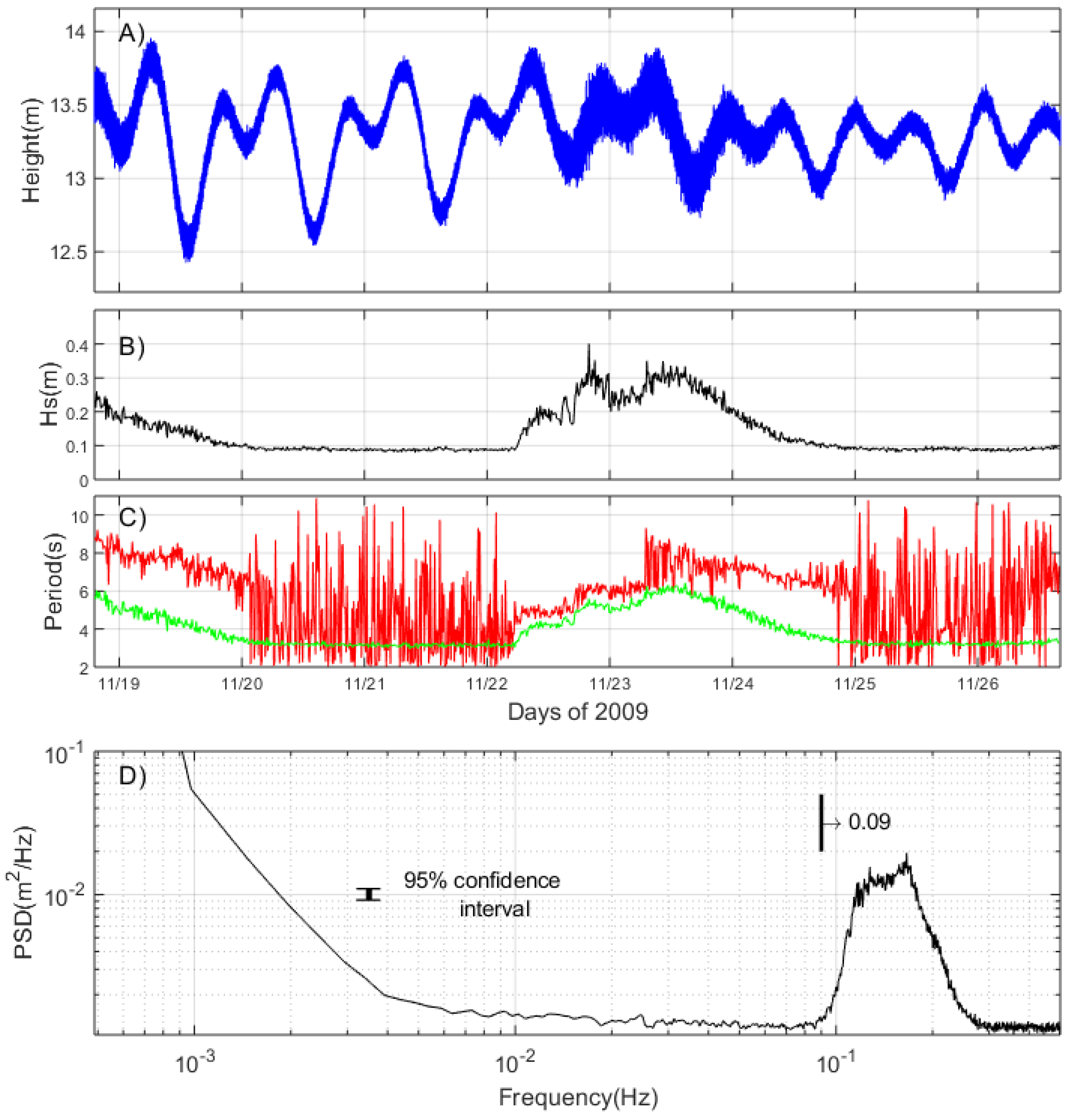
Wave bias is only partially removed with simple filtering approaches because waves often overlap in frequency range with turbulence [18]. The approach proposed here, the HA method, identifies wave harmonics from ADCP measurements by using Power Spectral Density (PSD) analysis and then fitting, via least squares [25], those harmonics identified from the PSD distribution to the ADCP measurements. The HA method is illustrated with a synthetic signal (Supplementary Material, Section 2) and with an approximately 8-day time series of sea surface height (m) and its PSD (m2/Hz) (Figure 1A,D). Wave energy is mostly distributed at frequencies higher than 0.09 Hz (Figure 1D). The highest significant wave height (Figure 1B) is approximately 0.4 m with a dominant period of 6 s at 20:00, on 22 November 2009. The dominant periods of the waves vary from 2 to 10 s, and the average periods change from 3 to 6.4 s (Figure 1C).
Frequencies associated with wave energy are identified from the PSD of the four beam velocities at the bin closest to the surface (top bin, 0.5 m thick). All wave frequencies identified from each PSD are then fitted to each of the four beam velocities for the top bin. This fit provides the amplitude and phase of the wave orbital velocities that are then reconstructed and subtracted from the beam velocities recorded by the ADCP.
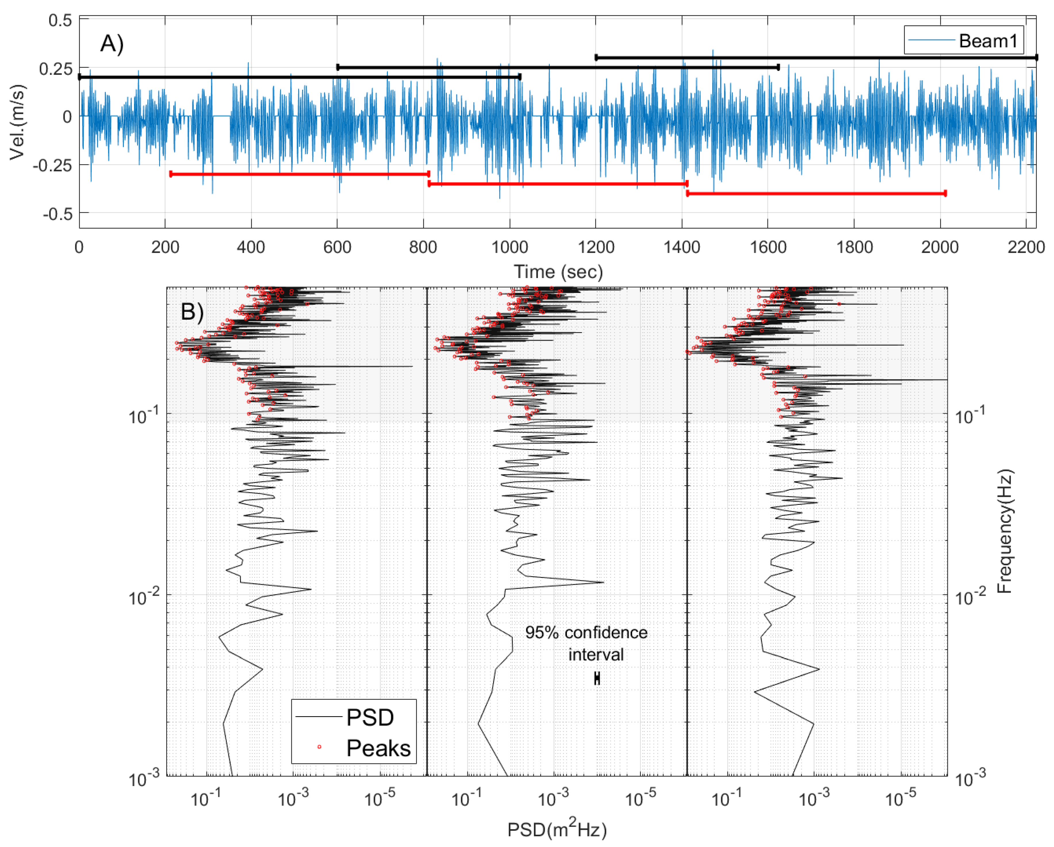
The HA method is applied to beam velocities because they resolve the rapidly changing orbital velocities better than the surface height. Details of the HA method are now illustrated with a segment (approximately 40 min) of the top-bin Beam1 velocity data (Figure 2A). The blue line is the top-bin Beam1 velocity measured at 1 Hz and the red lines delimit 600-s ensembles used to calculate turbulence parameters. Absolute values of pitch and roll tilts remained below 3 degrees throughout the deployment.
The HA method works under the assumption that turbulence is stationary for 10 min. Although PSDs can be estimated with 10-min ensembles, the actual PSDs are calculated with ensembles of 1024 samples (approximately 17 min or 1024 s) to avoid padding with zeros. Each PSD ensemble has overlaps of 424 s with each other, extending 212 s before and after each 10-min ensemble (e.g., Figure 2A). The black solid lines in Figure 2A indicate the window or ensemble size for the PSD calculation. The PSD for each black-line window of Figure 2A appears in Figure 2B. The shaded area in Figure 2B (frequencies > 0.09 Hz) denotes the wave-energy frequency band, which is the portion in need of wave-bias removal.
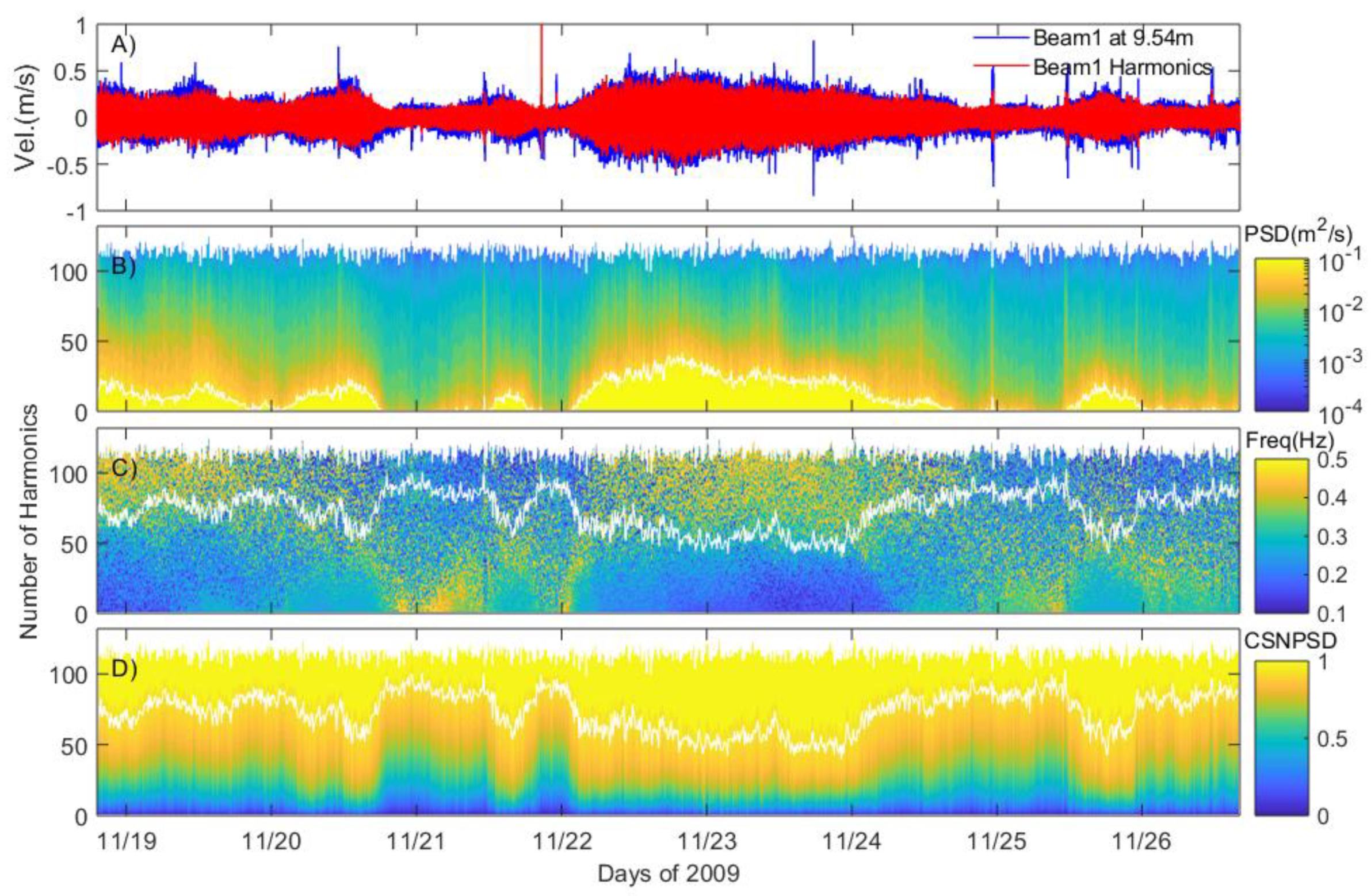
Subsequently, approximately 8 days of top-bin beam velocities (Figure 3A for Beam1) are used to calculate PSDs for all 10-min segments, as explained in Figure 2. The first step, after PSD calculation of each ensemble, is to find spectral peaks (red circles in Figure 2B) in the frequency range between 0.09 and 0.5 Hz. Each peak is assumed to be related to wave orbital velocities and identified as having larger spectral density than two neighboring values (please also see the Supplementary Material, Section 2). The next step is to sort the spectral peaks by descending order of spectral value (Figure 3B). This is done to identify X% of the wave energy, e.g., 95%, and remove it from the beam velocity. The vertical axis in Figure 3B–D indicates the number of peaks, or harmonics, identified in each 10-min ensemble. The shaded contour plot of sorted spectral peaks (Figure 3B) shows increased spectral energy at times with more harmonics containing the highest PSD (yellow-shaded areas). Increased spectral energies should appear at times of largest Beam1 velocity fluctuations (e.g., between 11/22 and 11/24; between 11/19 and 11/20; in the middle of 11/20; and in the second half of 11/25). The frequency corresponding to each sorted spectral peak is presented in Figure 3C. The largest spectral peaks between 11/22 and 11/24 correspond to frequencies between 0.1 and 0.2 Hz (blue regions in the contour plot). Similar frequency values are observed during other periods with largest variability in Beam1 velocity.
The following step is to remove X% of wave energy (e.g., 95%) from each 10-min ensemble. For this purpose, the PSDs are normalized with the sum of all spectral peaks (between 0.09 and 0.5 Hz) of that ensemble. In other words, each normalized PSD represents the ratio of each PSD value to the sum of all spectral peaks between 0.09 and 0.5 Hz. Then, normalized PSD values are integrated throughout all peaks of each 10-min ensemble to represent the Cumulative Normalized Power Spectral Density (CNPSD, Figure 3D). Thus, a value of 1 denotes 100% of the wave energy related to each ensemble. The white contour line in Figure 3C,D shows the number of peaks (or harmonics) representing 95% of the total wave energy from each ensemble (95% of the largest peaks in the PSDs of each ensemble). Overall, around 75 peaks represent 95% of the total energy of the peaks (Figure 3C,D). This number of peaks changes over time according to wave conditions. Relatively fewer spectral peaks contain 95% of the wave energy when the beam velocities are relatively higher. The crux of this method is to fit all harmonic frequencies, up to the white line, to each 10-min ensemble and thus obtain the amplitude and phase of each oscillatory harmonic, the wave signal. The fitted wave signal is finally subtracted from each 10-min beam velocity ensemble. This final procedure is as follows.
The wave orbital velocity may be represented by the sum of M harmonics plus a mean ():
where is an approximation to the wave orbital velocity of each 10-min ensemble. , , and are the amplitude, angular frequency, and phase, respectively, associated with the spectral peaks. Values of are gleaned from the PSD peaks of the beam velocity 10-min ensemble (Figure 3C). Values of u0, , and are obtained by fitting the harmonics to . For a more in-depth explanation of the least squares fit to Equation (17), see the Supplementary Material, Section 1. The harmonic orbital velocities are reconstructed with u0, , and from Equation (17) (red line in Figure 3A). This signal is taken as the wave orbital velocities , and then subtracted from the , i.e.,
The remaining signal (, or the difference between red and blue lines in Figure 3A) is assumed to be related predominantly to turbulent fluctuations and noise.
4. Comparison between VAF and HA Method
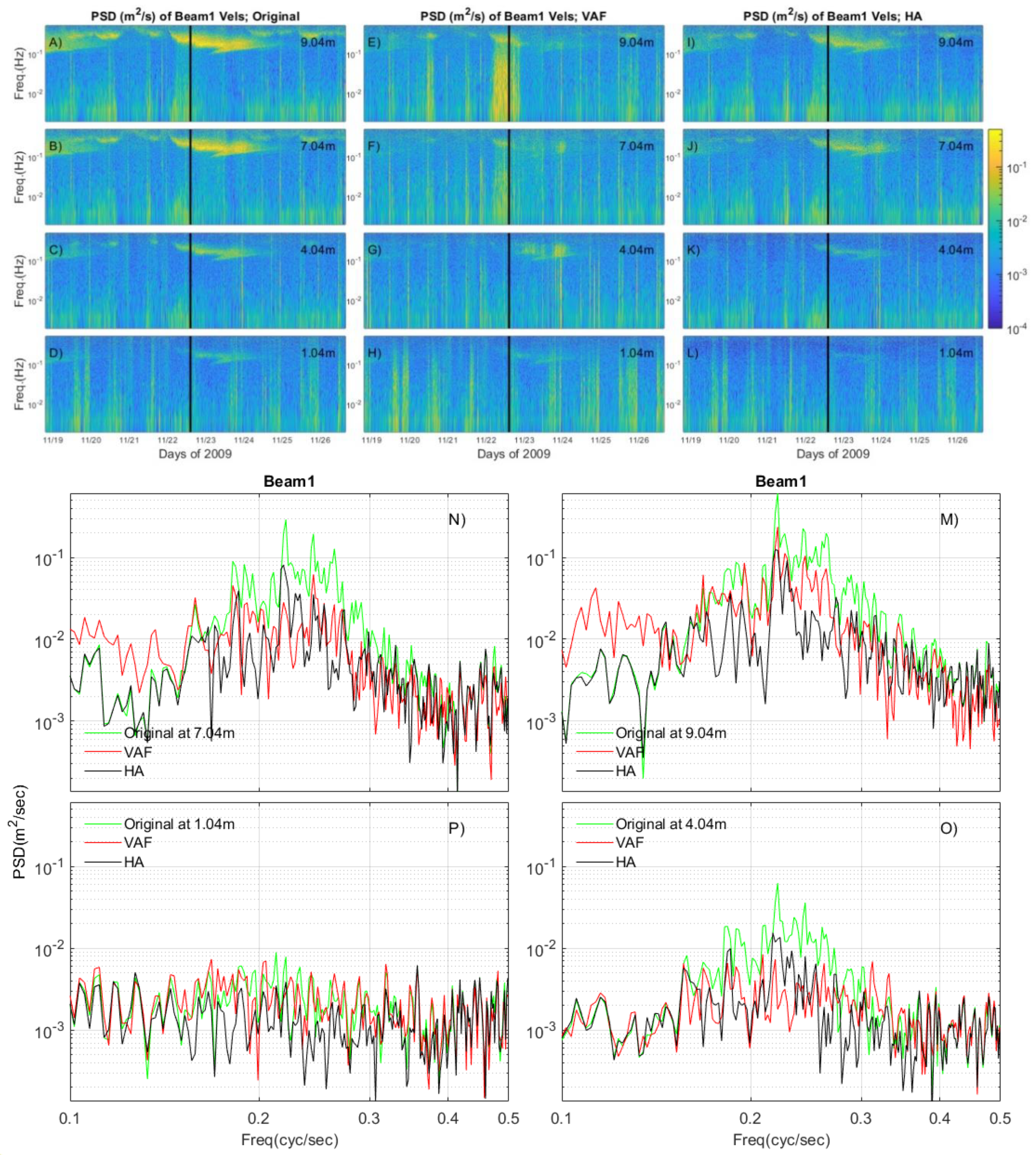
Power Spectral Densities derived from the VAF and HA methods are compared to the PSDs of original velocities over the entire water column for all 8 days of measurements (Figure 4). To evaluate the methods, PSDs are computed for every 10-min ensemble of the Beam1 velocities. The PSDs of original Beam1 velocities are shown in Figure 4A–D for different distances from the bottom. As shown in Figure 1B, surface gravity wave energy is predominantly distributed between 0.09 and 0.5 Hz, and it decreases with depth (Figure 4A–D). Surface gravity waves are evident between 11/19 and 11/21, evolving from low to high frequencies, and between 11/22 and 11/24, evolving from high to low frequencies. The shortest waves (>0.3 Hz) do not reach the bin closest to the bottom, while the longest waves (near 0.1 Hz) do reach those depths. This is expected from linear wave theory [26].
The PSDs corrected by VAF are shown in Figure 4E–H. A 2 m vertical separation is chosen to determine the continuous function in Equation (13), together with a 10-s window length for the weight function. Near the surface (9.04 m from the bottom, i.e., at the top bin) the VAF performs well at frequencies > 0.1 Hz. However, longer period waves are artificially amplified, especially between 11/22 and 11/23, when significant wave heights reach approximately 0.4 m (Figure 1B). The amplification of longer period waves also occurs at a distance of 7.04 m, although it is less prominent than near the surface. This artifact is caused by the least squares fit of the VAF method. Least squares Adaptive Filters amplify or generate signals, especially in longer period waves, to minimize the sum of squared residuals between two locations. Rosman et al. (2008) [18] explained that the linear transform does not sufficiently resolve the abrupt change of wave directions and phase difference between two locations during a 10-min averaging period. As a result, the VAF method does not perform well near the surface.
While the VAF method performs unreliably near the surface, the HA method removes most of the wave bias in the beam velocities (Figure 4I). The wave energy is drastically reduced between 0.09 and 0.5 Hz. Moreover, the VAF method loses vertical resolution at the surface because of its requirement to relate beam velocities at two locations. In this case, 2 m is used as the vertical separation to compute the linear function. Therefore, unbiased beam velocities are unattainable at 2 m below the surface. The wave energy is successfully removed at 1.04 m above the bottom (Figure 4L), but the VAF method generates pseudo-longer period waves in Figure 4H because VAF depends on the quality of the linear function [18] in Equation (13).
The wave signal removal by VAF and HA methods is illustrated on specific PSD plots (Figure 4M–P) corresponding to the black vertical lines of Figure 4A through L. Wave biases do not seem to be removed entirely between 11/22 and 11/24. However, the HA method reduces wave energies in the dominant peaks by approximately one order of magnitude relative to the original data. In addition, the wave energy resulting from the HA method is not amplified at low frequencies (<0.15 Hz), in contrast to the VAF method. This is particularly conspicuous in the signals at 7.04 m (Figure 4N) and 9.04 m (Figure 4M).
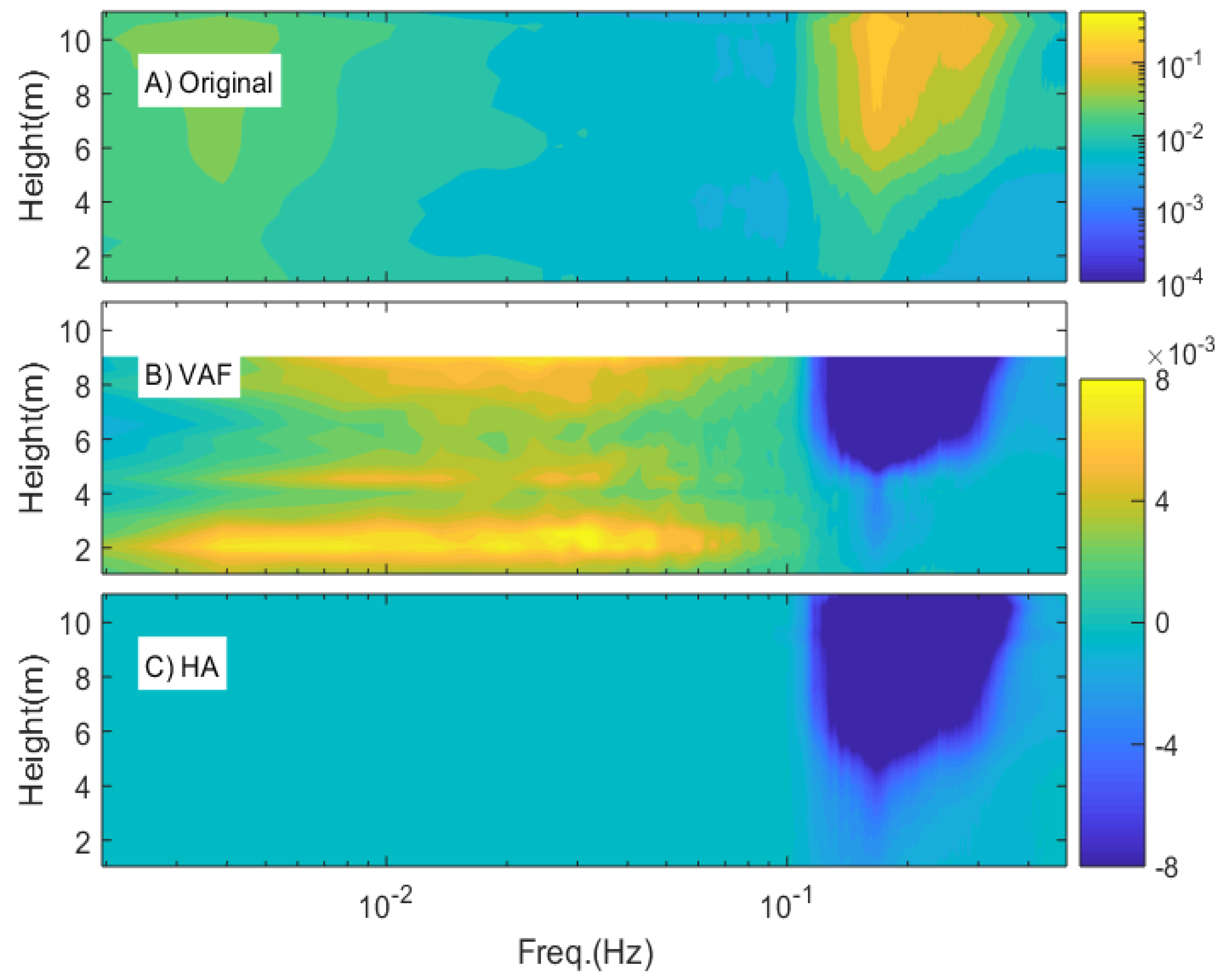
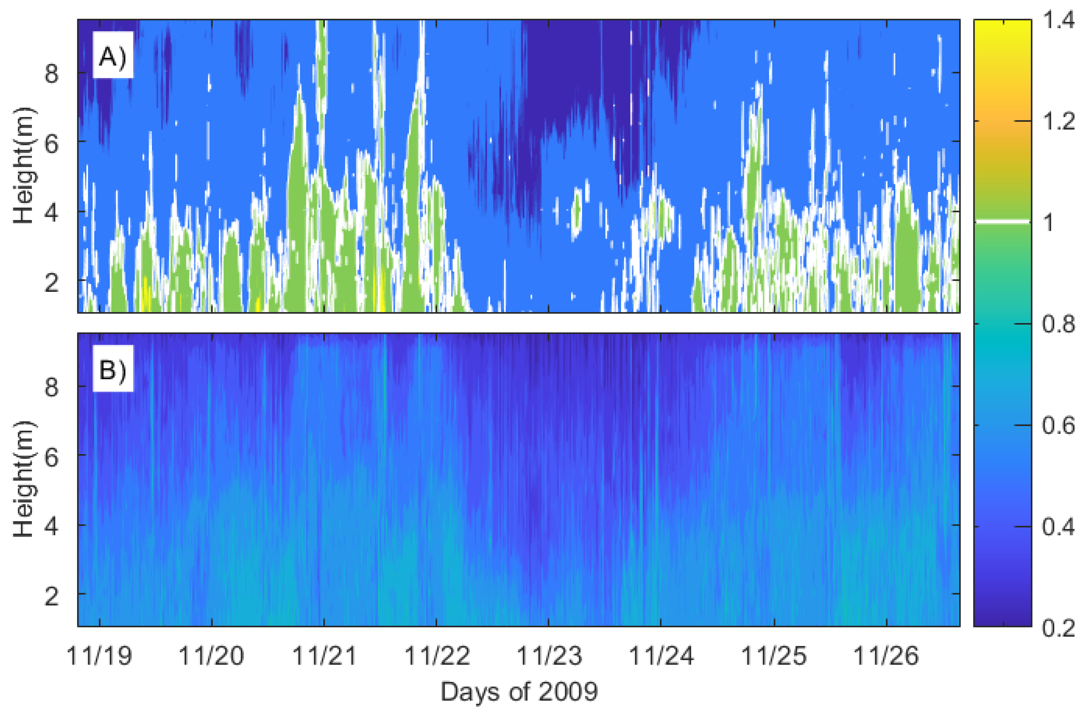
One way to evaluate the performance of the methods is to generate average PSD contours (Figure 5A) of all 10-min ensembles at each depth (Figure 4). The original average PSDs show wave energy predominantly at 0.17 Hz and at heights from the bottom above 5 m (Figure 5A). Deviations of the VAF and HA method from original ensemble-averaged PSDs are shown in Figure 5B,C, respectively. The deviations show that both VAF and HA methods remove the predominant wave energy at frequencies > 0.1 Hz. However, low-frequency wave energy is amplified with the VAF approach, especially at the surface and the bottom (Figure 5B). This is caused by the assumption that the wave velocity at A is a linear function of the wave velocity at B (Equation (13)). Wave velocities are unlikely to decay linearly with depth. The wave bias at frequencies > 0.1 Hz is approximately 10% less marked with the HA method than with the VAF. Moreover, spurious low frequency waves are not present in results obtained with the HA method (Figure 5C).
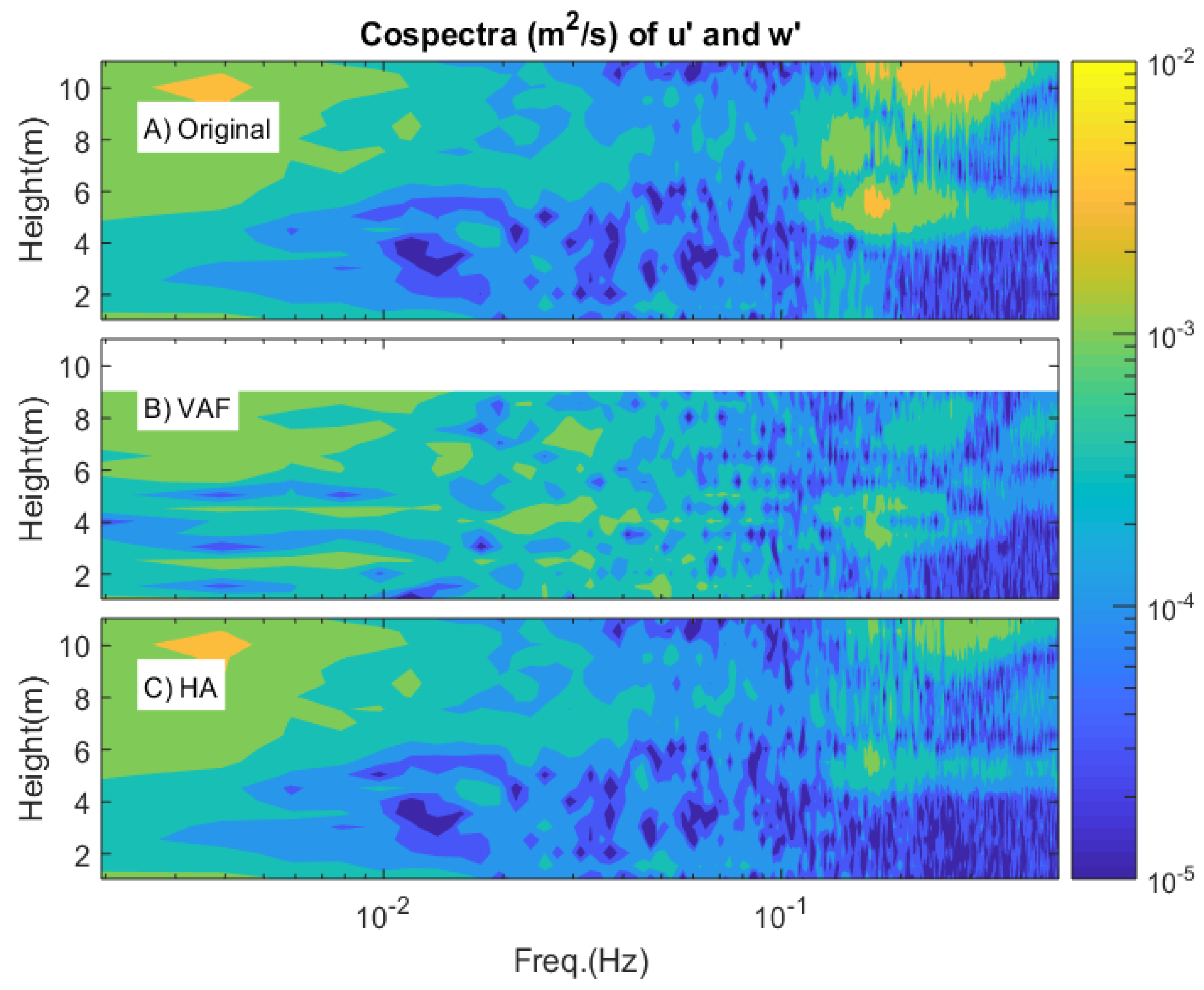
Another indicator of wave-bias removal is the cospectra of the beam velocities. Rosman et al. (2008) [18] indicated that the cospectra of and can be computed as
where and are the Power Spectral Densities of Beam1 and Beam2, respectively. The cospectra of original beam velocities have increased energy at the surface and in the middle of the water column at frequencies > 0.1 Hz (Figure 6A). As expected, the wave energy is highest at the surface and decreases with depth. In addition, increased wave energy appears at an approximately 5 m height. The VAF method performs well at frequencies > 0.1 Hz (Figure 6B) but loses vertical resolution as it relates velocities between two vertical positions to obtain the linear function described in Section 3. The cospectra computed by the HA method provides reasonable estimates at the surface (Figure 6C). Decreased cospectra indicated that the peaks where and have the same frequencies are largely removed. The magnitude of the HA method cospectra is approximately 64% and 36% smaller than the original cospectra at the surface and bottom, respectively.
5. Discussion
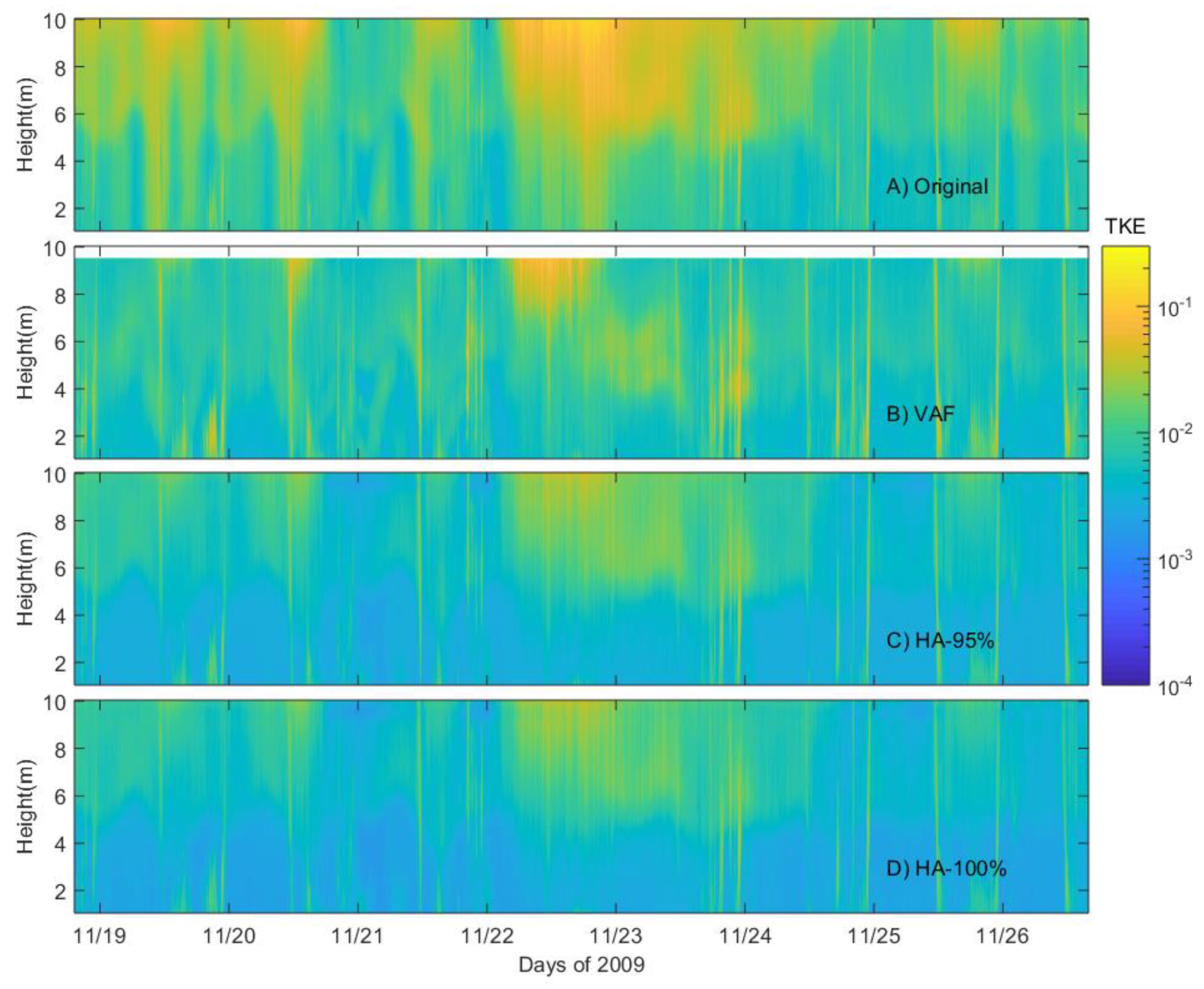
Turbulent Kinetic Energy was calculated with the original data and with the VAF and HA methods (Figure 7). The HA method was now applied by removing 95% and also 100% of the wave harmonics obtained from the PSD. The labels “HA-95%” and “HA-100%” in Figure 7C,D denote the Harmonic Analysis method that removes 95% and 100% of the wave energy. The sum of Turbulent Kinetic Energy (TKE) at 9.04 m was approximately 60% lower with the VAF method (Figure 7B) and approximately 67% lower with HA-95% (Figure 7C) relative to the original data. At 1.04 m, the TKE sum was approximately 24% less with the VAF method and approximately 55% less with the HA-95% method than with the original data. At 5.04 m, the TKE sum was approximately 34% less with the VAF method and approximately 63% less with the HA-95% method than that calculated with the original data (see also Table 1). The result of the TKE sum indicated that the HA method reduced more wave energy throughout the water column than the VAF method. Looking at the HA-100% approach, the TKE sum with HA-95% was approximately 15% more than the TKE sum with HA-100%. This shows a small change in the TKE budgets.
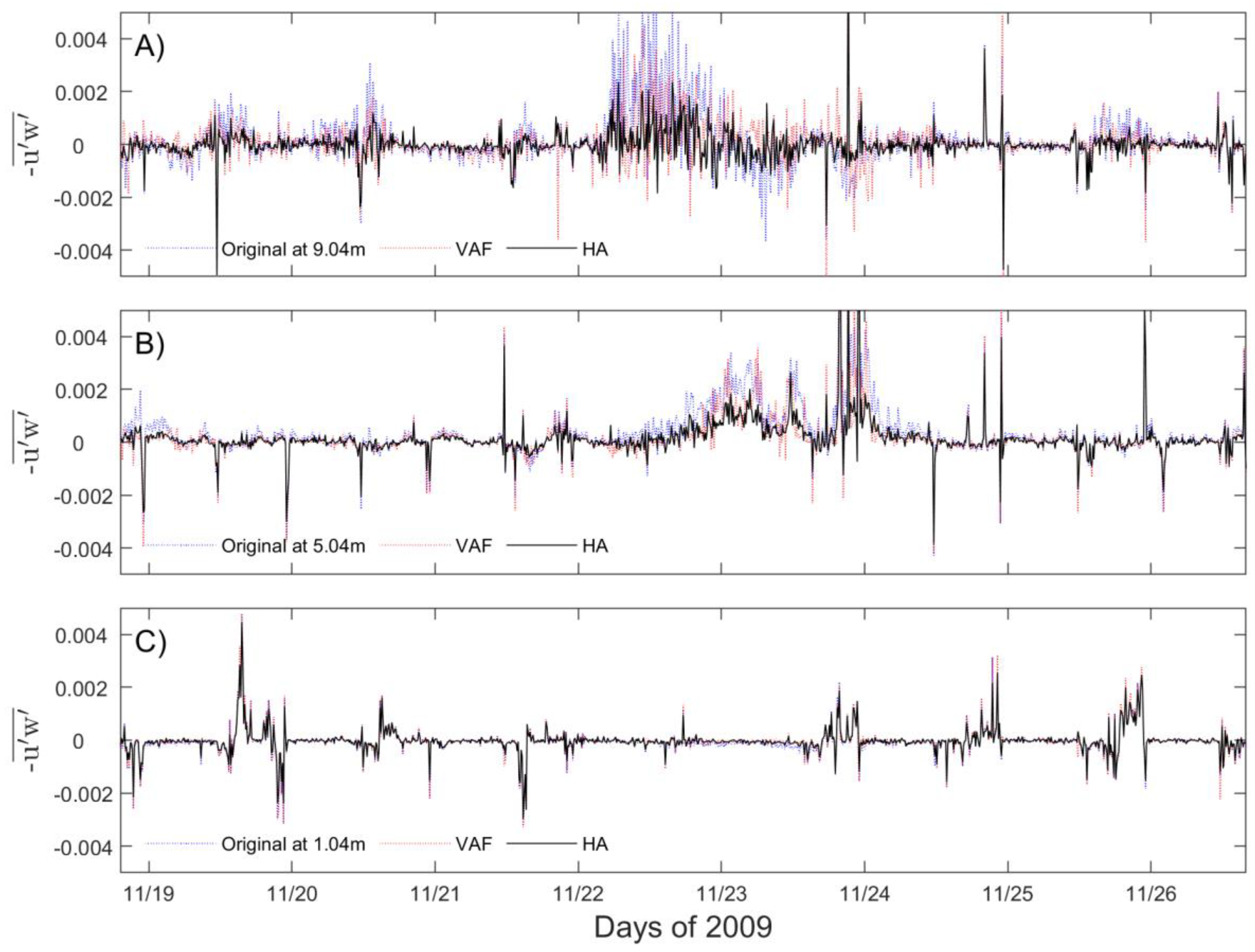
In addition, Reynolds stresses () were calculated with original velocities, with the VAF method and with the HA method at 3 different heights above the bottom (Figure 8). Compared to the original estimates and the VAF methods, the HA method gives the smallest standard deviation of Reynolds stresses at all depths. The standard deviation of Reynolds stresses for the HA method is approximately at 9.04 m (close to the surface) and at 1.04 m (closest to the bottom). Comparatively, the standard deviation of Reynolds stresses for the VAF method is approximately and at the same depths (Table 1). In other words, the Reynolds stresses standard deviation of the VAF method tends to be 50% greater than that of the HA method near the surface.
Furthermore, an estimate of the variance of Reynolds stresses () with the VAF method [18] is given by:
where denotes the estimator of the Reynolds stress. For comparison, the variance of Reynolds stresses can be estimated for the original velocity perturbations, for the VAF method, and for the HA method following Equation (20). In particular, standard deviations of Reynolds stresses derived from the VAF and HA methods are normalized with those obtained from the original velocities to compare the reliability of the VAF method with that of the HA method (Figure 9). Contour values >1 indicate that the estimator () of the VAF method is more broadly distributed than that of the original data (Figure 9A). Values > 1 from the VAF method are mostly found in the lower water column. This trend is caused by the difference between the velocity variance of the original beam velocities and the VAF method. As shown in Figure 4D,H, the Power Spectral Density for the original beam velocities is smaller than the Power Spectral Density for the VAF estimates. Based on the normalized standard deviation, the reliability in Reynolds stress estimates for the VAF method decreases toward the bottom of the water column. In contrast, contours of normalized standard deviations for the HA method are <1 everywhere (Figure 9B). This indicates that the reliability of the HA method increases in the entire water column, relative to the original estimates. The normalized standard deviations of the HA method are smallest at the top of the water column because the wave energy decreases with depth. Thus, the reliability of the Reynolds stresses is greater under relatively strong wave conditions (between 11/22 and 11/24) than under relatively weak wave conditions, as also noted in Figure 3A.
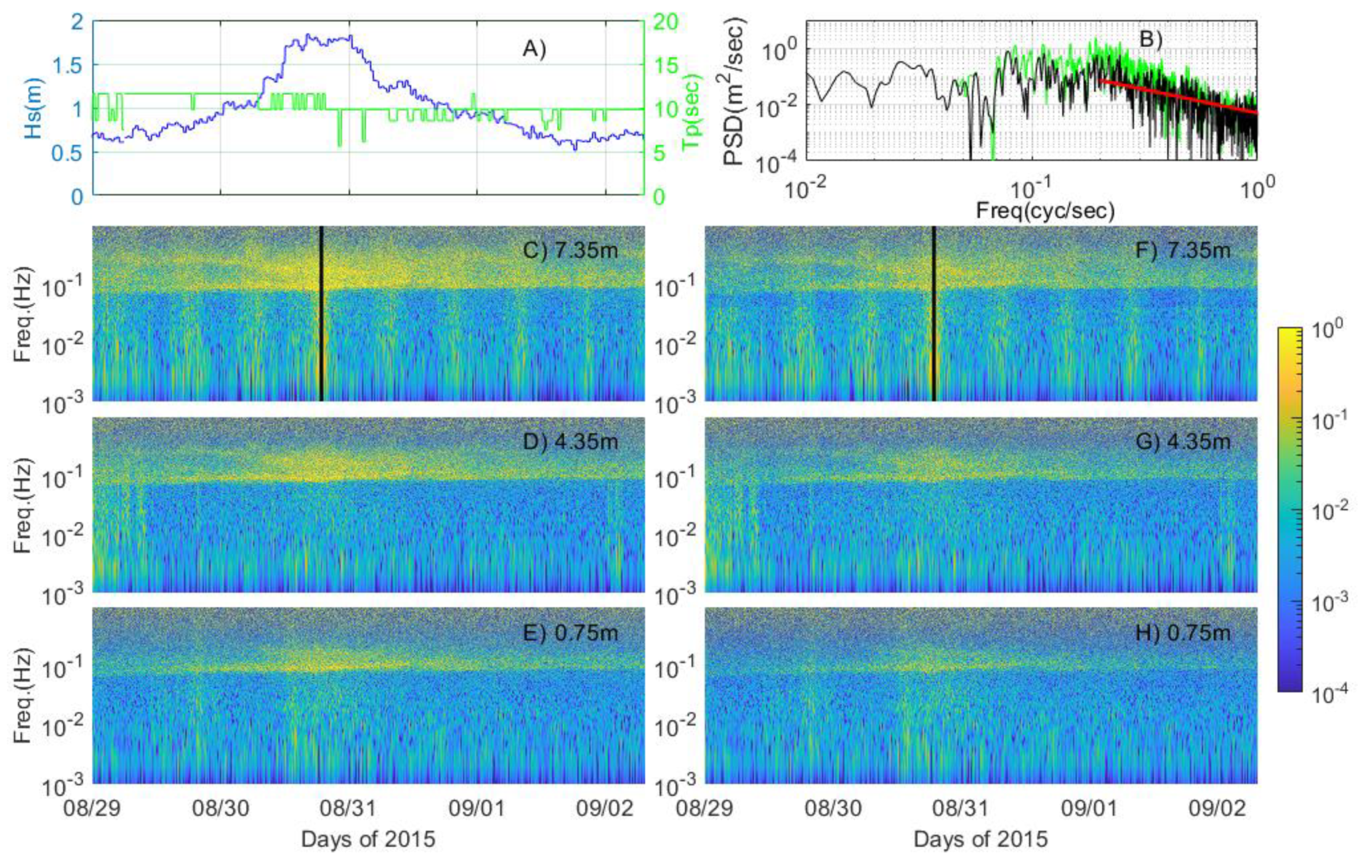
Rosman et al. (2008) [18] and Kirincich et al. (2010) [16] indicated that the VAF method is limited to mild wave climates, which would explain the difference with the HA method. To further evaluate the HA method in relatively more energetic wave conditions, the HA method is tested with a 4+ days, 2 Hz frequency dataset (Figure 10) over an approximately 8.5 m-depth water column near Cape Canaveral, Florida. The mean significant wave height (Hs) was approximately 1.0 m with a 10.2 s period. The highest significant wave height was 1.84 m with an approximately 12 s period at 16:05, August 30, 2015 (Figure 10A). The highest waves Hs > 1.5 m were steadily recorded from 11:30 on August 30 to 4:00 on August 31. The PSD of Beam1 velocity was estimated with a 10-min ensemble during the highest Hs (Figure 10B). The PSD of 95% wave-removed data (black line) decreases by approximately one order of magnitude at each peak identified, compared to the PSD of original data (green line). Moreover, the energy spectrum of the 95% wave-removed data cascades down with Kolmogorov’s −5/3 slope (red line, consistent with turbulence dissipation). Contours of PSD with 95% of waves removed show energy reduction at all depths (Figure 10F–H).
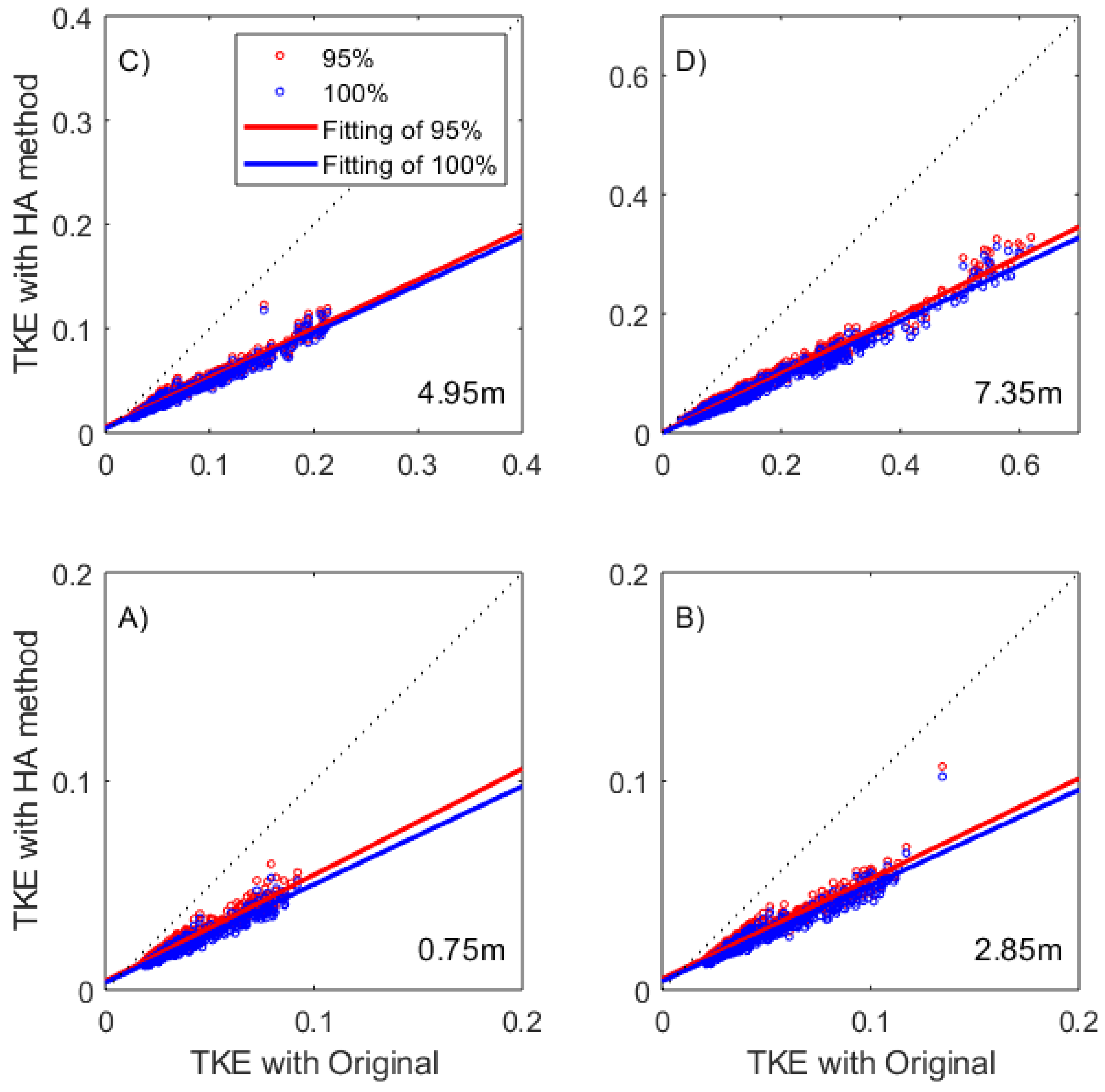
Turbulent Kinetic Energy estimated with 95% and 100% wave removal (for all depths) indicates the sensitivity of the method to the percentage of wave removal. This is assessed through a rough TKE budget (Figure 11). The black dotted line has a slope of 1. Data falling on that line would indicate no wave elimination from the total TKE budget. The red and blue circles denote that the HA method reduces wave energy from the total TKE because they fall below the straight line. Turbulent Kinetic Energy with corrected data is reduced by approximately 50% for every 10-min ensemble, compared with original data (Figure 11). The difference between a 95% and a 100% wave removal is determined by the linear fit lines (red and blue). The mean slope is approximately 0.02 larger for the 95% removal (red line) than the 100% removal (blue line). This indicates that the HA method of 100% wave removal reduces 2% more wave energy than the 95% wave removal. However, the time to reconstruct harmonics with HA-100% was 10.5 times longer than the time taken by HA-95%. In this study, the difference between HA-95% and 100% was barely noticeable. The user of the HA approach may determine the most convenient implementation of wave percentage to remove. From these results, the HA method performs well under energetic wave conditions and in the surface boundary layer, where the VAF method would be inadequate.
6. Conclusions
Recent progress has been made to remove wave contamination from ADCP velocity observations for improved estimates of turbulence properties. The Variance Fit method [13] and the VAF method [18] have had some success in “mild” wave climates [16]. Moreover, the CF method [16,19] has provided accurate derivations of Reynolds stress in the presence of surface gravity waves. The CF method relies on the assumption that the momentum in the atmospheric boundary layer is transferred to the upper ocean layer at a similar scale of the velocity cospectra. This approach can allow reduction of the wave bias under energetic wave conditions. However, the cospectra may be dissimilar in the middle of the water column, especially when buoyancy may exist via a pycnocline and show internal waves. In contrast, the HA method, introduced here, relaxes the assumptions and limiting conditions (restricted to relatively weak surface waves). The HA method consists of (a) using Power Spectral Densities to identify dominant wave harmonics and (b) applying Least Squares fits of ADCP beam velocities to those harmonics to identify the wave signal. This wave signal is subsequently subtracted from the ADCP beam velocities.
The estimation of Power Spectral Densities in Figure 4 shows that the HA method reduces wave-related spectral densities by one order of magnitude. The Turbulent Kinetic Energy estimates in Figure 7 compare original data to the VAF and HA methods. It is evident that the HA method reduces more wave energy than the VAF method. The sum of TKE at 9.04 m is 20% larger with the VAF method than with the HA-95% method. This is because the HA method separated more wave energy than the VAF method. Furthermore, the HA method performs well in energetic wave conditions (Hs > 1 m, Figure 10 and Figure 11). The HA method reduces approximately 50% TKE energy for every 10-min ensemble in energetic wave conditions. The and cospectra derived with the HA method near the surface and bottom are approximately 64% and 36% smaller than the original (wave-contaminated) cospectra. This implies that the wave energy of and is removed with the HA method. In addition, the HA method preserves the vertical resolution for the estimation of turbulence properties, while VAF loses vertical resolution as it relates velocities between two locations to obtain a required linear function.
Reynolds stress estimations and their reliability values show that the HA method performs better than the VAF method (Figure 8 and Figure 9). The Reynolds stress standard deviations derived with the HA method are approximately 45% and 16% smaller than the original data standard deviation near the surface and bottom, respectively. Reynolds stresses calculated near the bottom show similar values among the three estimates (original, VAF, and HA) because wave energy decays with depth. When compared via regression analysis (Figure 8, regressions not shown), the Reynolds stresses of the VAF method are consistent with those of the HA method only in the lower half of the water column. However, there is a discrepancy between the two methods near the surface. This is because the VAF does not perform well under energetic wave conditions [16]. Reliability analysis based on the standard deviation of the Reynolds stresses indicates that deviations of the HA method are smaller at all depths than the standard deviations from original estimates and from the VAF method. Therefore, the HA method should dramatically reduce wave contamination under surface and internal wave conditions. This approach should allow an improvement of estimates of the diffusive component of tracer transport by removing wind-wave effects that share spectral bands with turbulence. The diffusive transport of tracers is likely to develop throughout the world in nearshore regions, around tidal inlets, and in estuaries where wave action can influence transport processes.
Supplementary Materials
The following are available online at https://www.mdpi.com/2073-4441/12/4/1138/s1, Figure S1: (A) Ten-minute synthetic signals of turbulence (red), waves (blue) and waves plus turbulence (green). The green line would be analogous to an ADCP beam-velocity ensemble. This green line is the signal to which we want to remove the wave influence. (B) Power spectral density (PSD) of the waves+turbulence line in A) is shown in green, and the PSD of waves (blue line in A) is shown in blue, featuring the 10 harmonics prescribed. Figure S2: (A) The blue line is the same wave signal as in S1A and the red line is that reconstructed from fitting the frequencies identified by the PSD in S1B (green line) to the original signal (green line in S1A). (B) PSD of the turbulence prescribed in S1A (red line) and PSD of the turbulence, or signal, that arises from subtracting the red line in S2A from the original signal (green line in S1A). Figure S3: Same as in Figure S2 but using 95% of the wave energy from the PSD in Figure S1B (green line). Figure S2 uses 100% of the wave energy from the PSD in Figure S1B. As seen, the differnce between Figures S2 and S3 is minimal, as expounded in the main text with the actual records.
Author Contributions
Conceptualization, S.S., A.V.-L. and J.A.L.-C.; Data curation, S.S.; Formal analysis, S.S., J.A.L.-C., J.A. and M.A.-K.; Funding acquisition, A.V.-L.; Investigation, S.S. and A.V.-L.; Methodology, S.S.; Project administration, A.V.-L.; Resources, A.V.-L.; Supervision, A.V.-L.; Validation, J.A.-C., J.A. and M.A.-K.; Visualization, S.S. and J.A.L.-C.; Writing—original draft, S.S.; Writing—review & editing, A.V.-L. All authors have read and agreed to the published version of the manuscript.
Acknowledgments
We appreciate the efforts by Z. Biesinger and W. Lindberg in the instrument deployments and retrievals. This research was made possible in part by a grant from The Gulf of Mexico Research Initiative. AVL acknowledges support from NSF project OCE-1332718.
Conflicts of Interest
The authors declare no conflicts of interest.
References
- Smyth, W.D. Dissipation-range geometry and scalar spectra in sheared stratified turbulence. J. Fluid Mech. 1999, 401, 209–242. [Google Scholar] [CrossRef] [Green Version]
- Lewis, D. A simple model of plankton population dynamics coupled with a LES of the surface mixed layer. J. Theor. Boil. 2005, 234, 565–591. [Google Scholar] [CrossRef]
- Smith, K.M.; Hamlington, P.E.; Fox-Kemper, B. Effects of submesoscale turbulence on ocean tracers. J. Geophys. Res. Oceans 2016, 121, 908–933. [Google Scholar] [CrossRef] [Green Version]
- Tennekes, H.; Lumley, J.L. A First Course in Turbulence; MIT Press: Cambridge, MA, USA, 1972; p. 300. [Google Scholar]
- Burchard, H.; Petersen, O.; Rippeth, T.P. Comparing the performance of the Mellor-Yamada and the k-ϵ two-equation turbulence models. J. Geophys. Res. 1998, 103, 10543–10554. [Google Scholar] [CrossRef] [Green Version]
- MacKinnon, J.A.; Gregg, M.C. Mixing on the late-summer New England shelf—Solibores, shear, and stratification. J. Phys. Oceanogr. 2003, 33, 1476–1492. [Google Scholar] [CrossRef] [Green Version]
- Sharples, J.; Moore, C.M.; Abraham, E. Internal tide dissipation, mixing, and vertical nitrate flux at the shelf edge of NE New Zealand. J. Geophys. Res. Space Phys. 2001, 106, 14069–14081. [Google Scholar] [CrossRef]
- Simpson, J.H.; Crawford, W.R.; Rippeth, T.P.; Campbell, A.R.; Cheok, J.V.S. The Vertical Structure of Turbulent Dissipation in Shelf Seas. J. Phys. Oceanogr. 1996, 26, 1579–1590. [Google Scholar] [CrossRef] [Green Version]
- Williams, E.; Simpson, J.H. Uncertainties in Estimates of Reynolds Stress and TKE Production Rate Using the ADCP Variance Method. J. Atmos. Ocean. Technol. 2004, 21, 347–357. [Google Scholar] [CrossRef]
- Wiles, P.J.; Rippeth, T.P.; Simpson, J.H.; Hendricks, P.J. A novel technique for measuring the rate of turbulent dissipation in the marine environment. Geophys. Res. Lett. 2006, 33. [Google Scholar] [CrossRef]
- Lueck, R.G.; Huang, D.; Newman, D.; Box, J. Turbulence Measurement with a Moored Instrument. J. Atmos. Ocean. Technol. 1997, 14, 143–161. [Google Scholar] [CrossRef]
- Stacey, M.T.; Monismith, S.G.; Burau, J.R. Observations of turbulence in a partially stratified estuary. J. Phys. Oceanogr. 1999, 29, 1950–1970. [Google Scholar] [CrossRef]
- Whipple, A.C.; Luettich, R.A.; Seim, H.E. Measurements of Reynolds stress in a wind-driven lagoonal estuary. Ocean Dyn. 2006, 56, 169–185. [Google Scholar] [CrossRef] [Green Version]
- Whipple, A.C.; Luettich, R.A. A comparison of acoustic turbulence profiling techniques in the presence of waves. Ocean Dyn. 2009, 59, 719–729. [Google Scholar] [CrossRef]
- Shaw, W.J.; Trowbridge, J.H. The Direct Estimation of Near-Bottom Turbulent Fluxes in the Presence of Energetic Wave Motions. J. Atmos. Ocean. Technol. 2001, 18, 1540–1557. [Google Scholar] [CrossRef]
- Kirincich, A.; Lentz, S.; Gerbi, G.P. Calculating Reynolds Stresses from ADCP Measurements in the Presence of Surface Gravity Waves Using the Cospectra-Fit Method. J. Atmos. Ocean. Technol. 2010, 27, 889–907. [Google Scholar] [CrossRef]
- Trowbridge, J. On a Technique for Measurement of Turbulent Shear Stress in the Presence of Surface Waves. J. Atmos. Ocean. Technol. 1998, 15, 290–298. [Google Scholar] [CrossRef]
- Rosman, J.H.; Hench, J.L.; Koseff, J.R.; Monismith, S.G. Extracting Reynolds Stresses from Acoustic Doppler Current Profiler Measurements in Wave-Dominated Environments. J. Atmos. Ocean. Technol. 2008, 25, 286–306. [Google Scholar] [CrossRef]
- Gerbi, G.P.; Trowbridge, J.H.; Edson, J.B.; Plueddemann, A.J.; Terray, E.A.; Fredericks, J.J. Measurements of Momentum and Heat Transfer across the Air–Sea Interface. J. Phys. Oceanogr. 2008, 38, 1054–1072. [Google Scholar] [CrossRef] [Green Version]
- Scannell, B.; Rippeth, T.P.; Simpson, J.H.; Polton, J.; Hopkins, J.E. Correcting Surface Wave Bias in Structure Function Estimates of Turbulent Kinetic Energy Dissipation Rate. J. Atmos. Ocean. Technol. 2017, 34, 2257–2273. [Google Scholar] [CrossRef]
- Lohrmann, A.; Hackett, B.; Røed, L.P. High Resolution Measurements of Turbulence, Velocity and Stress Using a Pulse-to-Pulse Coherent Sonar. J. Atmos. Ocean. Technol. 1990, 7, 19–37. [Google Scholar] [CrossRef] [Green Version]
- Souza, A.; Howarth, M.J. Estimates of Reynolds stress in a highly energetic shelf sea. Ocean Dyn. 2005, 55, 490–498. [Google Scholar] [CrossRef] [Green Version]
- Nidzieko, N.J.; Fong, D.A.; Hench, J.L. Comparison of Reynolds Stress Estimates Derived from Standard and Fast-Ping ADCPs. J. Atmos. Ocean. Technol. 2006, 23, 854–861. [Google Scholar] [CrossRef] [Green Version]
- Kaimel, J.C.; Wyngaard, J.C.; Izumi, Y.; Coté, O. Spectral characteristics of surface-layer turbulence. Q. J. R. Meteorol. Soc. 1972, 98, 563–589. [Google Scholar] [CrossRef]
- Thomson, R.E.; Emery, W.J. Data Analysis Methods in Physical Oceanography, 3rd ed.; Elsevier: Amsterdam, The Netherlands, 2014; p. 716. [Google Scholar]
- Dean, R.G.; Dalrymple, R.A. Water wave mechanics for engineers and scientists. Adv. Ser. Ocean Eng. 1991, 2, 353. [Google Scholar]
Figure 1.
Data from the northeastern Gulf of Mexico, in the Florida Big Bend region. (A) Time series of water surface height (m), (B) Significant wave heights (Hs), (C) Dominant wave period (DPD) in red and Average wave period (APD) in green, and (D) Power Spectral Density (m2/Hz) of the time series shown in (A).

Figure 2.
(A) Beam1 velocities at 9.04 m above the bottom (blue line) during a 37-min segment. Data windows to compute Power Spectral Density (PSDs) (m2/s, black lines), and ensembles used to calculate Reynolds stresses (, red line). (B) PSDs calculated with the data windows denoted by black lines in (A); the shaded area indicates the frequency band in need of wave-bias removal. The red circles denote peaks at the frequencies identified to reconstrut wave signals.

Figure 3.
(A) Beam1 velocities (blue line) and wave orbital velocities (red line) computed by the Harmonic Analysis (HA) method; (B) PSDs (m2/s) of the peaks sorted by descending order; and 0.08 PSD (m2/s) in the white line (C) Frequencies corresponding with the sorted PSDs and (D) Cumulative Sum of Normalized Power Spectral Density (CNPSD). In both C and D, the white line represents the number of harmonics with 95% energy.

Figure 4.
PSD (m2/s) of original Beam1 velocities (m/s) at (A) 9.04 m, (B) 7.04 m, (C) 4.04 m, and (D) 1.04 m above the bottom; PSD of Beam1 velocities of the Vertical Adaptive Filtering (VAF) method at (E) 9.04 m, (F) 7.04 m, (G) 4.04 m, and (H) 1.04 m and PSD of Beam1 velocities of the HA method (I) 9.04 m, (J) 7.04 m, (K) 4.04 m, and (L) 1.04 m. Line plots: (M–P), show the PSD corresponding to the black vertical line in the contour plots.

Figure 5.
(A) Time-averaged PSD (m2/s) as a function of height above bottom with original Beam1 velocities. (B) Difference between the VAF method and the original time-averaged PSD. (C) Difference between the HA method and original time-averaged PSD.
Figure 5.
(A) Time-averaged PSD (m2/s) as a function of height above bottom with original Beam1 velocities. (B) Difference between the VAF method and the original time-averaged PSD. (C) Difference between the HA method and original time-averaged PSD.

Figure 6.
Time-averaged cospectra (m2/s) of and (A) original; (B) corrected by VAF method; and (C) corrected by HA method.
Figure 6.
Time-averaged cospectra (m2/s) of and (A) original; (B) corrected by VAF method; and (C) corrected by HA method.

Figure 7.
Turbulent Knetic Energy (TKE) estimated by (A) Original data, (B) VAF, (C) HA method with 95% wave energy removed, and (D) HA method with 100% wave energy removed.
Figure 7.
Turbulent Knetic Energy (TKE) estimated by (A) Original data, (B) VAF, (C) HA method with 95% wave energy removed, and (D) HA method with 100% wave energy removed.

Figure 8.
Reynolds stresses () computed by original data (blue dotted line), VAF method (red dotted line), and HA method (black solid line) at (A) 9.04 m; at (B) 5.04 m; and at (C) 1.04 m.
Figure 8.
Reynolds stresses () computed by original data (blue dotted line), VAF method (red dotted line), and HA method (black solid line) at (A) 9.04 m; at (B) 5.04 m; and at (C) 1.04 m.

Figure 9.
Standard deviation (A) of VAF method Reynolds stress estimates () and (B) of HA method Reynolds stress estimates, normalized by that of original Reynold stress estimates. The white line represents the value 1.
Figure 9.
Standard deviation (A) of VAF method Reynolds stress estimates () and (B) of HA method Reynolds stress estimates, normalized by that of original Reynold stress estimates. The white line represents the value 1.

Figure 10.
Data from a shoal off Cape Canaveral, Florida. (A) Significant wave heights (Hs) with a blue solid line marked on the left of the y-axis and dominant wave period (TP) marked on the right of the y-axis. (B) The PSD corresponding to the black vertical line in (C) and (F). The green and black line denotes the PSD of original data and 95% wave-removed data, respectively. Red line is a reference line for –5/3. The PSD of original data are shown (C) at 7.35 m, (D) at 4.35 m, and (E) at 0.75 m height. The PSD of 95% wave-removed data are given (F) at 7.35 m, (G) at 4.35 m, and (H) at 0.75 m height.

Figure 11.
Comparison of TKE with original data to TKE with the HA method (A) at 0.75 m, (B) at 2.85 m, (C) at 4.95 m, and (D) at 7.35 m. Red and blue circles denote the estimation of 95% and 100% wave-removed data, respectively. Red and blue solid lines denote the corresponding linear-fitting line of the estimations. Black dotted line indicates the reference line of equilibrium between TKE with original data and TKE with the HA method.


Table 1.
Performance indicators of wave-removal methods in the estimates of turbulence parameters at different distances from the bottom. The HA method was more effective in reducing wave-related values of Turbulent Kinetic Energy (TKE) and Reynolds stress than the VAF method.
Table 1.
Performance indicators of wave-removal methods in the estimates of turbulence parameters at different distances from the bottom. The HA method was more effective in reducing wave-related values of Turbulent Kinetic Energy (TKE) and Reynolds stress than the VAF method.
| Method | TKE (% Reduction) | Reynolds Stress (Standard Dev × 10−3 m2/s2) | |||
|---|---|---|---|---|---|
| 1.04 m | 5.04 m | 9.04 m | 1.04 m | 9.04 m | |
| VAF | 24 | 34 | 60 | 0.55 | 0.87 |
| HA | 55 | 63 | 67 | 0.46 | 0.58 |
© 2020 by the authors. Licensee MDPI, Basel, Switzerland. This article is an open access article distributed under the terms and conditions of the Creative Commons Attribution (CC BY) license (http://creativecommons.org/licenses/by/4.0/).
Share and Cite
MDPI and ACS Style
So, S.; Valle-Levinson, A.; Laurel-Castillo, J.A.; Ahn, J.; Al-Khaldi, M. Removing Wave Bias from Velocity Measurements for Tracer Transport: The Harmonic Analysis Approach. Water 2020, 12, 1138. https://doi.org/10.3390/w12041138
AMA Style
So S, Valle-Levinson A, Laurel-Castillo JA, Ahn J, Al-Khaldi M. Removing Wave Bias from Velocity Measurements for Tracer Transport: The Harmonic Analysis Approach. Water. 2020; 12(4):1138. https://doi.org/10.3390/w12041138
Chicago/Turabian StyleSo, Sangdon, Arnoldo Valle-Levinson, Jorge Armando Laurel-Castillo, Junyong Ahn, and Mohammad Al-Khaldi. 2020. "Removing Wave Bias from Velocity Measurements for Tracer Transport: The Harmonic Analysis Approach" Water 12, no. 4: 1138. https://doi.org/10.3390/w12041138
Note that from the first issue of 2016, this journal uses article numbers instead of page numbers. See further details here.