Analyses of Precipitation and Evapotranspiration Changes across the Lake Kyoga Basin in East Africa


Department of Civil and Building Engineering, Kyambogo University, P.O. Box 1, Kyambogo, Kampala, Uganda
*
Author to whom correspondence should be addressed.
Water 2020, 12(4), 1134; https://doi.org/10.3390/w12041134
Submission received: 15 March 2020
/
Revised: 10 April 2020
/
Accepted: 15 April 2020
/
Published: 16 April 2020
(This article belongs to the Special Issue Assessment of Spatial and Temporal Variability of Water Resources)
Abstract
:This study analyzed changes in CenTrends gridded precipitation (1961–2015) and Potential Evapotranspiration (PET; 1961–2008) across the Lake Kyoga Basin (LKB). PET was computed from gridded temperature of the Princeton Global Forcings. Correlation between precipitation or PET and climate indices was analyzed. PET in the Eastern LKB exhibited an increase (p > 0.05). March–April–May precipitation decreased (p > 0.05) in most parts of the LKB. However, September–October–November (SON) precipitation generally exhibited a positive trend. Rates of increase in the SON precipitation were higher in the Eastern part where Mt. Elgon is located than at other locations. Record shows that Bududa district at the foot of Mt. Elgon experienced a total of 8, 5, and 6 landslides over the periods 1818–1959, 1960–2009, and 2010–2019, respectively. It is highly probable that these landslides have recently become more frequent than in the past due to the increasing precipitation. The largest amounts of variance in annual precipitation (38.9%) and PET (41.2%) were found to be explained by the Indian Ocean Dipole. These were followed by precipitation (17.9%) and PET (21.9%) variance explained by the Atlantic multidecadal oscillation, and North Atlantic oscillation, respectively. These findings are vital for predictive adaptation to the impacts of climate variability on water resources.
1. Introduction
Within the River Nile basin, Lake Kyoga links Lake Victoria to Lake Albert. However, the Lake Kyoga Basin (LKB) is the least studied among the River Nile tributaries [1]. This is due to lack of quality observed long-term hydrometeorological data. Generally, in the sub-Saharan Africa (where the LKB is located), weather stations are of low density, unevenly distributed, and not continuously operational due to poor maintenance of data recording equipment or instruments [2]. In some cases, studies tend to be conducted using short-term data. For instance, to investigate the groundwater–surface water interactions of papyrus wetlands in the LKB, Southwell [3] used data observed from July 2015 to February 2016. Such short-term data cannot be representative of the long-term variation in the hydrometeorology.
Generally, to circumvent the problem of lack of historical long-term series, studies tend to make use of the reanalyses or remotely sensed datasets. A few examples of precipitation products and/or temperature datasets freely available to researchers can be obtained from the Princeton Global Forcings (PGFs) [4], Global Precipitation Climatology Project (GPCP) [5], Climatic Research Unit (CRU) [6], African Rainfall Climatology (ARC) [7], Tropical Rainfall Measuring Mission (TRMM) [8], and Climate Forecast System Reanalysis (CFSR) of the National Centers for Environmental Prediction (NCEP) [9]. The temperature from some of the freely downloadable datasets can be used to estimate Potential Evapotranspiration (PET). Several studies (for instance, [10,11,12,13]) that made use of the freely available precipitation products. The main advantage of reanalyses data is that they tend to be of a large (or global) spatial scale.
In hydrology, hydrometeorology, and perhaps other fields, precipitation and evapotranspiration are respectively the first and second largest terms in relation to the water budget. Especially for the estimation of PET, several studies [14,15,16,17,18,19] made use of remotely sensed and/or satellite images. Glenn et al. [14] in their review put emphasis on studies that combine methods for estimating evapotranspiration from remote sensing and ground observations considering areas such as agricultural region, rangelands, and natural ecosystems. Vinukollu et al. [15] compared the performance of a single source energy budget model, Penman–Monteith approach, and Priestley–Taylor method for estimating evapotranspiration at a global scale. Where soil evaporation plays a dominant role, the Priestley–Taylor approach and the single source energy budget model yielded results, which were highly comparable with ground-based observations of evapotranspiration; however, the Penman–Monteith method showed the highest correlation for sensible heat flux [15]. Bashir et al. [19] assessed the applicability of evapotranspiration estimates from remotely sensed data for managing of Gezira Scheme in Sudan. Alemu et al. [17] investigated the association between evapotranspiration and vegetation dynamics in the River Nile basin. Liou and Kar [18] conducted a review of evapotranspiration estimation with remote sensing and a number of surface energy balance algorithms. For the study area, Nsubuga et al. [20] used remotely sensed Landsat images for 1986, 1995, and 2010 to detect changes in the surface water area of the LKB. Nsubuga et al. [20] showed that the surface area of Lake Kyoga was increasing. Such findings are relevant for applications, which directly depend on the Lake Kyoga and its outflow. The main challenge with remotely sensed data or satellite images is that they tend to be of short term. Furthermore, acquiring an archive of such imagery with high spatial and temporal resolution is always very expensive. Therefore, given that in the analyses of trends and variability, long-term data are required, reanalyses data can be used based on the intended applications or the purpose for which the study is being conducted.
There are a number of water resources applications within the LKB. Some of these applications include the 600 Mw Karuma hydro power plant (located shortly downstream of the Lake Kyoga outflow), as well as the several irrigation schemes such as Agoro, Doho, and Olwenyi in Lamwo, Butaleja, and Lira Districts, respectively. In Bududa district, which is located in the Eastern part of the LKB, the occurrence of precipitation-induced landslides is common. The recent landslide occurred in December 2019 [21]. Therefore, for an insight on the variation in the water budget of the LKB, it is important to assess precipitation and PET changes in terms of long-term trends, and/or multidecadal variability. Whereas long-term trends may be due to global warming, precipitation and PET decadal or multidecadal variability can be to a number of drivers. Such drivers can include the changes in large-scale ocean–atmosphere conditions, as well as the influence from regional and local factors. Dry and wet conditions across the East Africa where the LKB is located can be linked to the increase or decrease in the Sea Surface Temperature (SST) or atmospheric pressure at the sea level across the various oceans. When precipitation or PET variability drivers are known, an upcoming period of wet or dry condition can be predicted thereby supporting planning of predictive adaptations to the impact of climate variability on water resources, and agriculture.
This study aimed at analyzing precipitation and PET trends and variability across the LKB. This, while focusing on the rainy season as well as annual time scale, was done while investigating the possible linkage of the precipitation and PET variability to the changes in large-scale ocean–atmosphere conditions.
2. Materials and Methods
2.1. The Study Area
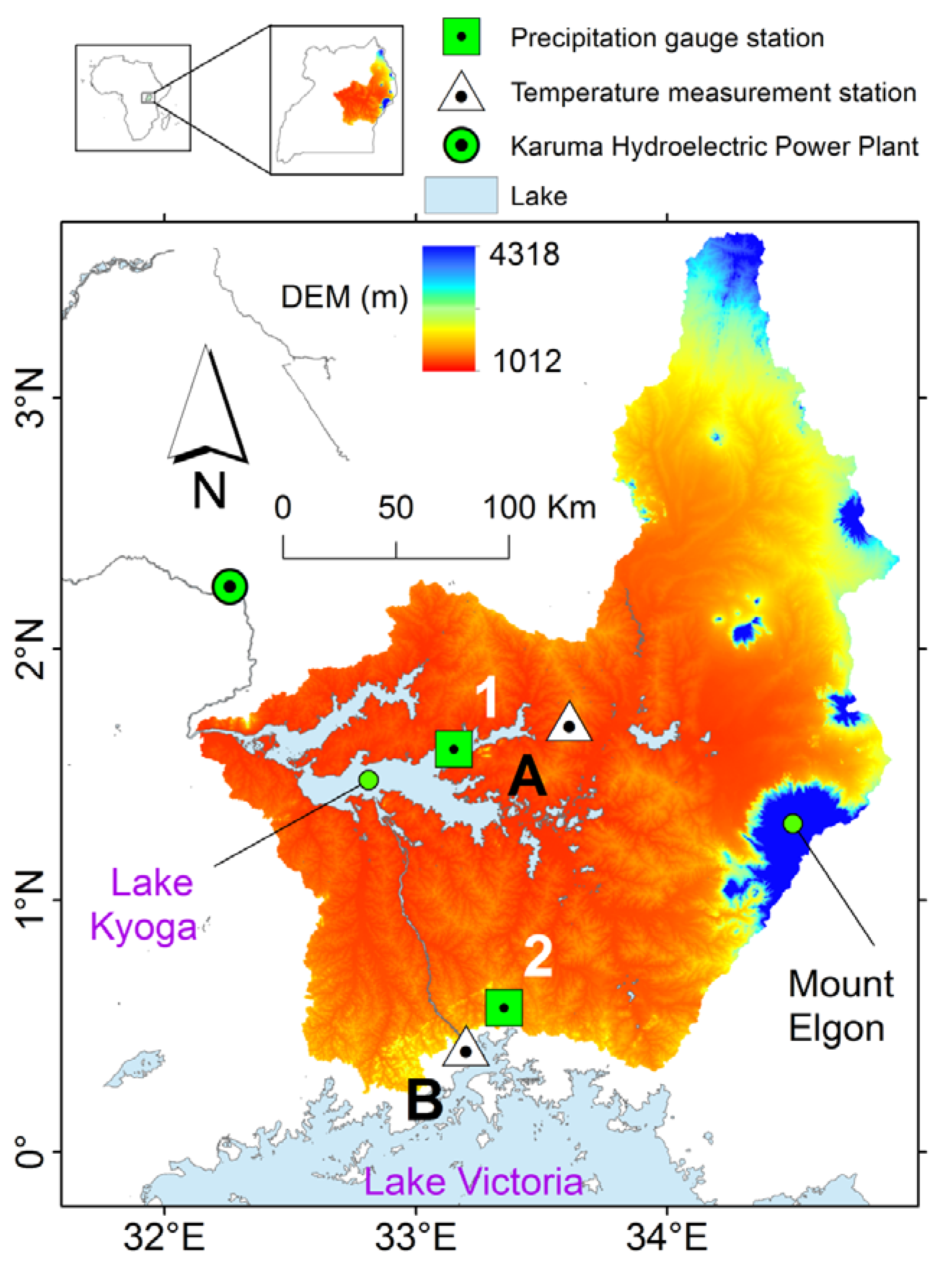
The LKB is found in the upper part of the River Nile Basin. It is located in Uganda, a country found in East Africa. Apart from Lake Kyoga, the LKB comprises Lake Bisina and Lake Nakuwa with the open water surface areas of 130 km2 and 83 km2, respectively [22]. The Lake Kyoga receives flows from the Victoria Nile and the tributaries emanating from the Mount Elgon region. The Lake Kyoga is shallow (with most parts less than 4 m deep) but connects Lake Victoria to Lake Albert. The drainage area of the LKB has been reported differently by many researchers as 75,000 km2 [23], 57,233 km2 (Food and Agriculture Organization FAO [24]), and about 57,000 km2 [1,25]. Nevertheless, the drainage area of the LKB stretches between 0° N and 4° N (in the North–South direction) and 32° E and 35° E (in the East–West direction). The vast drainage area of the LKB is exclusively within the confines of the territorial boundary of Uganda. The study area starts from the central part of the country and extends through the eastern region until the northeastern subregion. The LKB consists of eleven subcatchments including Awoja, Okok, Okere, Mpologoma, Victoria Nile, Sezibwa, Akweng, Abalang, Lwere, Lumbuye, and Kyoga Lake side zones (Figure 1). There are a number of ethnic tribes found within the LKB including (among others) the Buganda, Busoga, Iteso, Kumam, Jopadhola, Sebei, Lango, and Karamojong. The main occupation of the people in the LKB is subsistence farming. Fishing is another key occupation especially for those close to the shoreline of the Lake Kyoga. However, in the far northeastern part of the LKB, the Karamojongs are nomadic pastoralists and tend to move from place to place in search for pasture and water for their livestock.
In Figure 1, the background map of the LKB is the Digital Elevation Model (DEM). The hole-filled DEM derived from the USGS/NASA [26] and processed by the International Centre for Tropical Agriculture (CIAT-CSI-SRTM) using interpolation methods described by Reuter et al. [27] was downloaded online via the link http://srtm.csi.cgiar.org (accessed: 3 December 2019). It is noticeable that the elevation ranges from about 1000 to 4320 m above sea level. The highest point (4320 m) is the peak of Mount Elgon located in the Eastern part of the LKB. The lowest lying area is in the Teso subregion where the slope of the terrain hardly exceeds 2%. The difference between the highest and the lowest point across the study area is large (up to about 3310 m).
The long-term (1961–2000) mean annual rainfall at the two selected precipitation gauge Stations 1 and 2 was found to be 1436 mm and 1258 mm, respectively. At the selected locations A and B, the observed Tmin values for each month were above 18 °C. Therefore, based on the Koppen Geiger classification [28,29], the climate of the LKB is characterized by Af or Equatorial fully humid climate (along the equator) and Aw or Equatorial savannah with the dry (December–January–February, DJF) season in the northeastern part.
2.2. Data
Data from various sources were used in this study. The data included precipitation, PET, and climate indices. Regarding the selection of the data period for analyses, it is vital to note that in 1960 there was a step jump in the precipitation mean in the region where the LKB is located. To eliminate the influence of step jump in the precipitation mean on results of trend analyses, data over the periods before and after the step jump are required to be considered separately. Eventually, to reflect the recent variability in precipitation and PET across the LKB, the period 1961–2015 was selected.
2.2.1. Precipitation
Gridded (0.3° × 0.3°) monthly precipitation of CenTrends v1.0 data [30] was downloaded via the link https://doi.org/10.1038/sdata.2015.50 (accessed: 25 May 2019). There were no missing records in the gridded data over the selected period 1961–2015.
Daily rainfall data from 1961 to 2000 observed at Bugaya labeled as Station 1 (longitude = 33.15, latitude = 1.60) in Figure 1 was obtained from the Uganda National Meteorological Authority (UNMA). Monthly rainfall data over the period 1961–2000 observed at Ivukula labeled as Station 2 (longitude = 33.35, latitude = 0.57) in Figure 1 was adopted from a previous study [25] after quality control had already been performed. In other words, data at Station 2 had no missing records. However, the missing records at Station 1 were infilled based on the linear relationship between data of corresponding months at Stations 1 and 2.
For trend and variability analyses, the monthly CenTrends precipitation was converted to seasonal and annual scales. Similarly, the observed precipitation was converted to seasonal and annual scales. Comparison of long-term mean monthly values of observed and CenTrends precipitation was made (see Figure 2). It is noticeable that the mismatch between the observed and CenTrends precipitation was minimal for both Stations 1 and 2 (Figure 2a,b). This close agreement between the two datasets was because the CenTrends data were obtained by Kriging interpolation of observed precipitation. Therefore, a possible difference between observed and CenTrends precipitation would be due to the influence of the few number of weather stations in the region where LKB is located on the interpolation estimates. Nevertheless, amidst low density of weather stations in a region (like in the sub-Saharan Africa where the study area is located), the empirically determined distance decay functions are required to control the Kriging procedure.
It can be seen that the precipitation at Station 2 clearly shows a bimodal pattern with peaks in the March–April–May (MAM) and September–October–November (SON) seasons while December–January–February (DJF), and June–July–August (JJA) periods were dry. The precipitation pattern tends to rely on the migration of the Inter-Tropical Convergence Zone (ITCZ) in response to the pressure differences in the south and northern hemispheres. This is because a band of precipitation tends to move with the ITCZ as it migrates from the south to the north or vice versa. The ITCZ crosses the equator twice a year, firstly while it is migrating northwards from the southern hemisphere, and secondly during its southward retreat after reaching close to 20° N. The first and second crossing of the equator leads to the MAM and SON precipitation (for instance at Station 2), respectively. An important note is that in June, July, and August, the ITCZ is clearly in the northern hemisphere. Eventually, the area (farther away from the equator but close to 20° N) gets continuous precipitation in the JJA season. In other words, the farther one gets Northwards of Equator, the more unimodal the monthly precipitation pattern becomes. This explains why the JJA season has more precipitation at Station 1 than that at Station 2.
2.2.2. Temperature and PET
Gridded (0.5° × 0.5°) daily minimum (Tmin) and maximum (Tmax) temperature were obtained from Princeton Global Forcing (PGFs) [4] via the link http://hydrology.princeton.edu/data/pgf/ (accessed: 27th June 2019). The PGF data covered the period 1948–2008. To conform to the period for precipitation, the PGF Tmin and Tmax used in this study were over the period 1961–2008.
Daily Tmin and Tmax observed at Soroti and Jinja labeled as Station A (longitude = 33.611, and latitude = 1.715), and Station B (longitude = 33.204, and latitude = 0.423), respectively (see Figure 1), were obtained from the UNMA. The available data obtained for Station A covered the period 1971–1974. At Station B, daily data was available over the periods 1961–1982 and 1983–2000. Station A had no missing values. Station B had a missing record of 4%. Infilling of the missing records for a particular month was done through the arithmetical mean. For instance, the missing record for 1st November, 1978 was obtained as the average of values recorded on every 1st November in 1977, 1976, 1979, and 1980. This method was adopted for Station B because there were no available nearby temperature measurement stations for this study.
Several methods exist for the estimation of PET including the FAO Penman-Monteith (FPM) method [31], Makkink method [32], Hargreaves method [33,34], Blaney–Criddle approach [35], and Priestley–Taylor method [36]. Generally, the methods for PET estimation can categorically be based on temperature [33,35], radiation [32,36], mass transfer [37], combined energy, and mass balance [31]. Comparison of the various PET estimation methods has been widely made in several studies such as [38,39,40,41]. Each of the PET estimation methods has its advantages and disadvantages. The FPM method is physically based and gives the most realistic estimates of PET across various climates [31]. However, the application of the FPM in a data scarce region (like where the LKB is located) is limited due to its huge data requirements. Makkink, Blaney–Criddle, and Priestley–Taylor methods require local calibration of some of their parameters and this affects the PET estimates. The Hargreaves method [33,34] is simple to compute, has low data requirement (in terms of only Tmax, Tmin, and latitude) to estimate PET of a location. Chuanyan et al. [42] compared three methods for estimating PET including Behnk–Maxey [43], Prestley–Taylor [36], and Hargreaves [33,34]. The Hargreaves method was found to be the best for areas where weather stations were sparse [42]. In this line, furthermore, given that only Tmin and Tmax were available, the Hargreaves method [33,34] was adopted for the computation of the PET in this study such that
where PET is in mm/day, Tmin and Tmax are in (°C), Tmean refers to the mean air temperature (°C), and Ra denotes the extra-terrestrial solar radiation (W/m2). The Ra can be computed in terms of latitude. Equation (1) was applied to the Tmin and Tmax at each grid point. Furthermore, the PET was converted from daily to monthly scale. Like the temperature data, the PET series used in this study covered the period 1961–2008.
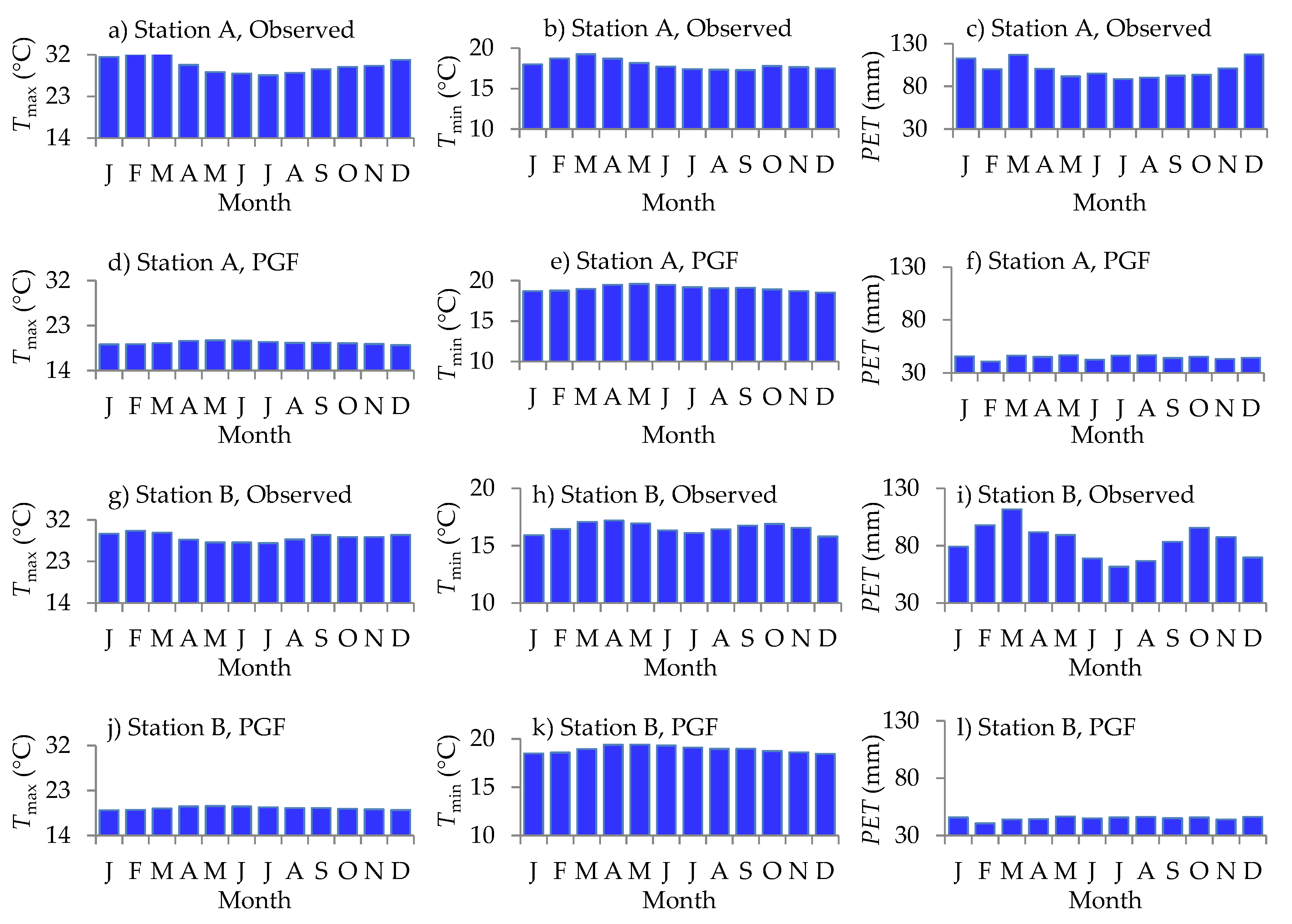
For comparison, the PGF data (Tmin and Tmax) were extracted at Stations A and B. Comparisons of observed and PGF-based temperature (Tmin and Tmax) as well as the PET were made (Figure 3). For clarity taking the differences in the orders of magnitudes of the variables, plots for observed and PGF-based Tmin, Tmax, and PET were made separately. At Station A, the observed temperature exhibited peaks twice a year (a bimodal pattern) though it is more clearly visible for Tmax than Tmin (Figure 3a,b). Nevertheless, at Station A, the maximum temperatures occurred during the DJF season. For the PGF data (Figure 3a,b), there was one peak (a unimodal pattern). The differences between Tmax and Tmin were larger for observed than PGF data. Eventually, the observed PET (Figure 3c) of each month was largely underestimated by the PGF-based PET (Figure 3f). At Station B or close to the equator, Tmin, Tmax, and PET (Figure 3g–i) were clearly of a bimodal pattern with the peaks during the MAM and SON seasons. However, the PGF-based Tmin and Tmax exhibited a unimodal pattern (Figure 3j–k). On average, the monthly mean values of the observed Tmax and Tmin were 27.53 °C and 16.54 °C, respectively. However, PGF-based Tmax and Tmin yielded a monthly mean of 19.46 °C and 18.91 °C, respectively. In other words, the PGF data underestimated the observed differences between Tmax and Tmin (an aspect that comprised of an important component of Equation (1)). Eventually, the deviation of the PETs of the various months from the monthly mean was larger for observed (Figure 3i) than PGF-based data (Figure 3l). In other words, (i) the response of the PET to rainy seasons (MAM, JJA, SON, and DJF) was not well captured by the PGF data, and (ii) for each month, the PGF-based PET were only about 50% of the observed PETs.
2.2.3. Climate Indices
A number of monthly climate indices including the North Atlantic oscillation (NAO), Atlantic multidecadal oscillation (AMO), Niño 3 index, and the Indian Ocean dipole index (IOD) were obtained from various sources.
- (a)
- The NAO index [44,45] is the normalized pressure difference between a station on the Azores and one on Iceland. Monthly NAO index was obtained from http://www.esrl.noaa.gov/psd/gcos_wgsp/Timeseries/NAO/ (accessed: 30 June 2019). The data used in this study covered the period 1960–2015.
- (b)
- The AMO index is defined as the SST averaged over 25–60° N, 7–70° W minus the regression on the global mean temperature [46]. The monthly AMO index [47,48] was obtained from https://www.esrl.noaa.gov/psd/gcos_wgsp/Timeseries/AMO/ (accessed: 30 June 2019). The data used in this study covered the period 1960–2015.
- (c)
- The Niño 3 [48,49] is the area averaged SST for the Tropical Pacific region 90° W to 150° W and 5° N to 5° S. The monthly Niño 3 data was obtained via http://www.esrl.noaa.gov/psd/gcos_wgsp/Timeseries/Nino3/index.html (accessed: 25 May 2019). The Niño 3 covered the period 1960–2015.
- (d)
- The IOD is the climate mode associated with the state of the SST over Western (50° E to 70° E and 10° S to 10° N) Equatorial and Southeastern (90 to 110° E and 10° S to 0° N) Indian Ocean [50]. The monthly IOD series obtained from the Japan Agency for Marine-Earth Science and Technology (JAMEST) via the link http://www.jamstec.go.jp/frcgc/research/d1/iod (accessed: 20 January 2014) and used in the research by Onyutha and Willems [51] was adopted from this study. The IOD used in this study covered the period 1960–2003.
Precipitation and PET were converted to seasonal and annual timescales. For the relevance of water resource applications, apart from the annual precipitation and PET, wet conditions in each year or MAM, and SON rainy seasons were considered.
2.3. Trend
Trend analysis is normally two-fold. The trend magnitude or slope is first computed. In this line, the trend slope (m) in MAM, SON, and annual precipitation and PET was computed using the method of Theil [52] and Sen [53]. The second step requires testing of the significance of the non-zero slope of a linear variation of the variable. Trend significance can be tested parametrically or non-parametrically. Linear regression test is parametric and requires the data to be normally distributed. The assumption that the data should be normally distributed is not necessary for non-parametric methods including the Mann–Kendall (MK; [54,55]), and Spearman Rho (SR; [56,57,58]) tests. However, both the MK and SR tests are specifically for trend detection. Therefore, in this study, another non-parametric approach that tests both trends and variability was adopted. In other words, the significance of the trend was tested in terms of the difference between the exceedance and non-exceedance counts of data points [59,60,61]. Examples of recent studies that applied the method adopted in this study include Pirnia et al. [62], Tang and Zhang [63], Vido et al. [64], and Cengiz et al. [65]. Statistically, the comparability of the adopted method with the MK test was demonstrated in previous studies [2,59].
In the adopted method, the given data X of sample size n is first transformed into series d using [59,60,61].
where,
Increasing and decreasing trends are indicated by T > 0, and T < 0, respectively. The distribution of T is approximately normal with the mean of zero and the variance = (n − 1)−1 such that [60,61].
where Z is the standardized trend statistic with the mean of zero and variance equal to one while β is a factor to correct the variance of T from the influence of autocorrelation on Z. The suitability of β for analyses of autocorrelated data can be found demonstrated by Onyutha [13]. Let Zα/2 denote the standard normal variate at a selected α. The null hypothesis H0 (no trend) is not rejected if |Z| < Zα/2 at α; otherwise, the H0 is rejected.
The trend test was applied to the precipitation and PET at each grid point. Spatialization of trend results across the study area was achieved through interpolation. Another method of spatialization is regionalization, an approach that requires division of the study area into homogenous regions. Regionalization was not relevant for this study. Several methods exist for spatial interpolation such as ordinary kriging, inverse distance weighted interpolation, and universal kriging. Ordinary kriging was adopted in this study because it allows for the optimization of interpolation estimates using distance decay functions thereby making it possible to limit the area of influence of each station to some reasonable value. The kriging method is important for Africa (where the study area is located), since large areas are ungauged, and values from the edges of these un-monitored locations can perpetuate thousands of kilometers when not constrained [30].
2.4. Variability
Variability in the MAM, SON, and annual precipitation, and PET was computed in terms of subtrends based on Equation (6) following the approach of Onyutha [2]. If we consider X to have a subset x from the uth to the vth value of X, Equation (6) can be applied based on a subseries extracted using the window (of length w) moved from the start to the end of the series. For the selected w, t = 0.5 × (w + 1) and t = 0.5 × w in the cases when w is odd and even, respectively, such that
where Zi is the ith value of Z, while the terms u and v can be given by:
Based on the values from Equation (7), the plot of Zi against the corresponding ith data year can be used to diagnose the variability in the data. Due to natural randomness, over one epoch, the subtrends can be positive while a subsequent subperiod can be characterized by negative subtrends. The Z = 0 line can be taken as the reference corresponding to the case when there is completely no trend in the data. The occurrence of positive and negative subtrends in a clustered way in time characterizes the variability in the data. The H0 (natural randomness) is rejected if the scatter points (in the plot of Zi against the corresponding ith data year) go outside the (100 − α)% Confidence Interval (CI) limits or |Z| > Zα/2 at the selected α. However, if the scatter points fall within the (100 − α)% CI limits, the H0 (natural randomness) is not rejected at the selected α.
2.5. Correlation Analysis
The covariation of the subtrends in the seasonal and annual precipitation with climate indices was determined in terms of correlation. The H0 (no correlation between the subtrends of precipitation and those of the climate indices) was tested at α = 0.05 (at each grid point). This step was repeated for the climate indices and PET. The idea was to determine the amount of variance in precipitation or PET that could be explained in terms of the changes in large-scale ocean–atmosphere interactions.
3. Results
3.1. Trend
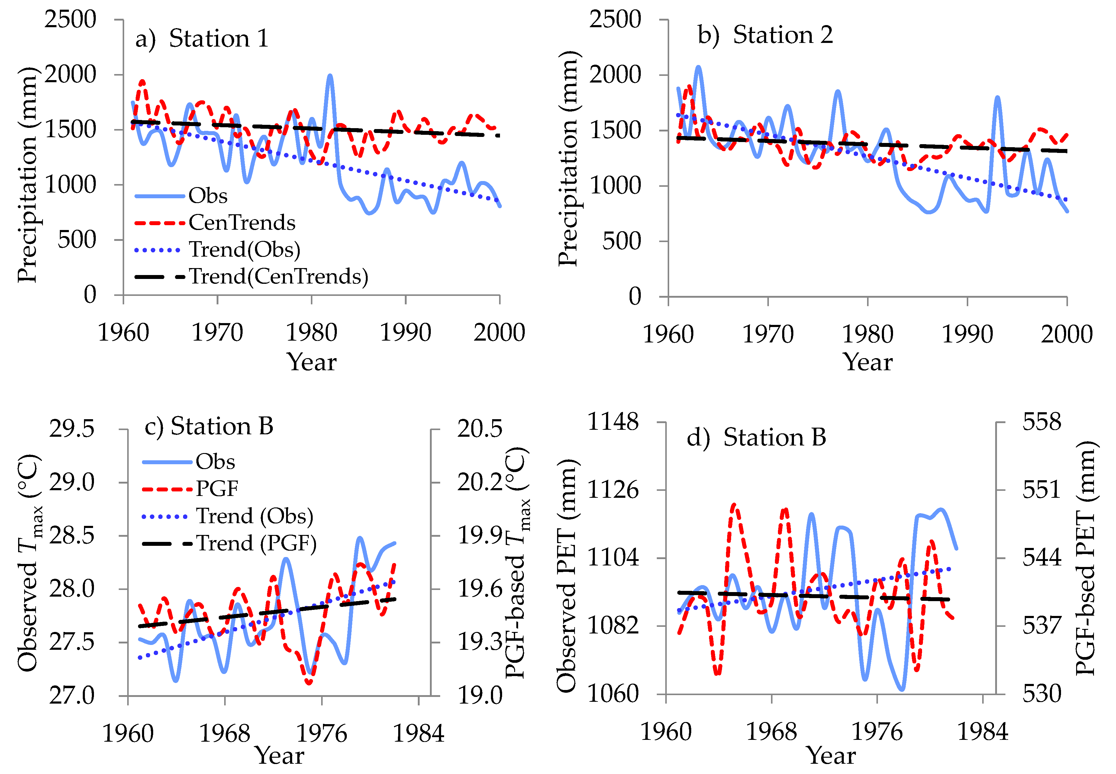
Figure 4 shows linear trends fitted to annual precipitation, Tmax and PET. Both observed and CenTrends-based annual precipitation (Figure 4a,b) exhibited a decrease. The corresponding trend slopes at Station 1 were −18.257 mm/year, and −3.2168 mm/year, with p = 0.001 and p = 0.423, respectively. At Station 2, trend slopes in observed and CenTrends-based precipitation were −19.567 mm/year, and −3.0809 mm/year, with p = 0.006 and p = 0.631, respectively. In other words, the precipitation decrease with time was faster in observed than the CenTrends data. In Figure 4c, Tmax was considered because it is important in the computation of PET using temperature-based method (see Equation (1)) as adopted in this study. At Station B, both observed and PGF-based annual Tmax (Figure 4c) exhibited an increase. The rate of increase of Tmax was 0.0339 °C/year and 0.0072 °C/year for observed and PGF-based temperature, respectively. From Figure 4d, there were contrasting trend slopes of 0.6508 mm/year and −0.0345 mm/year in observed and PGF-based PET, respectively. As seen from Equation (1), PET depends on the difference between Tmax and Tmin. For each data year, the difference between Tmax and Tmin was larger for observed than PGF data. Though only shown for annual time scale, the differences in trends between observed and CenTrends precipitation varied among seasons. Furthermore, observed and PGF-based temperature (or PET) trends also tended to differ among seasons. It is envisaged that the differences in trends between observed and CenTrends precipitation, as well as observed and PGF-based PET may vary in magnitude from one location to another across the LKB. Nevertheless, the use of CenTrends precipitation and PGF-based PET in this study was to give an insight on the possible long-term trend, something that is important for planning predictive adaptation of water resources management.
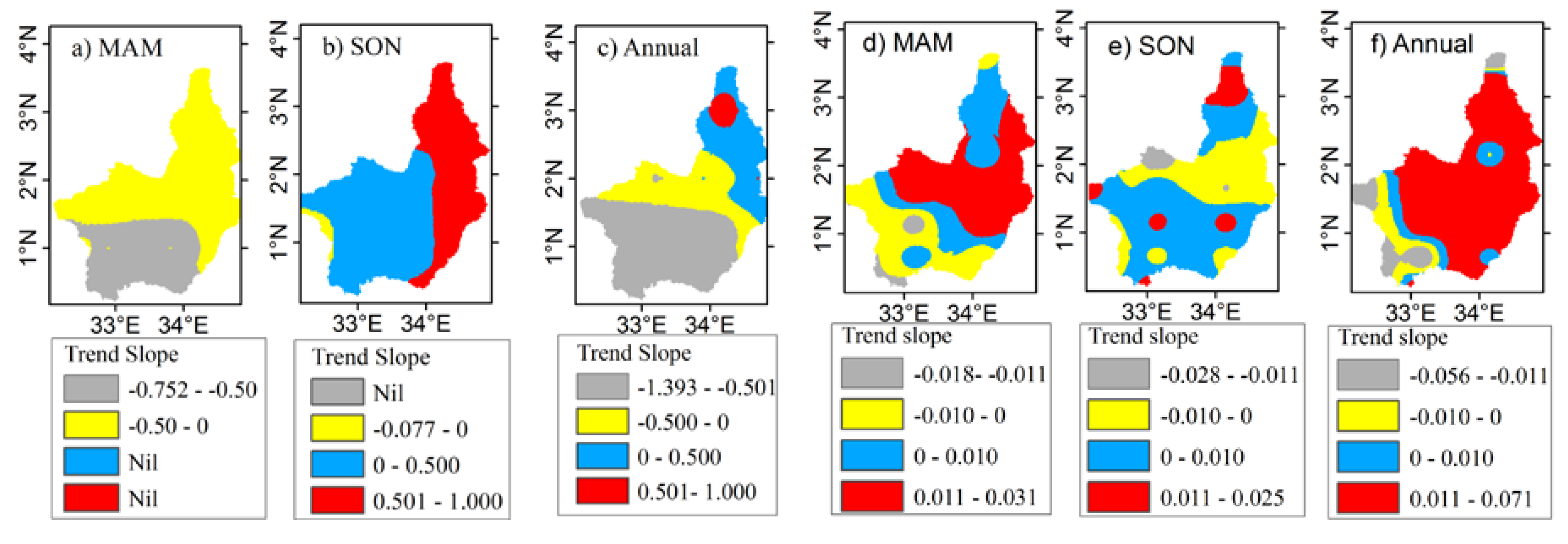
Figure 5 shows magnitudes of statistical trends in precipitation and PET. The corresponding Z values for the significance of the trends can be found in Figure A1 of Appendix A. At the selected α of 0.05, the Zα/2 = 1.96. The southern part of the LKB exhibited a decreasing trend in both MAM (Figure 5a) and annual (Figure 5c) precipitation. For the eastern part of the LKB, SON precipitation exhibited an increase (Figure 5b). The trend slope in the southern part of the LKB was as low as −0.752 mm/year, −0.078 mm/year, and −1.393 mm/year for MAM (Figure 5b), SON (Figure 5d), and annual (Figure 5f) precipitation, respectively. For these negative trends, the H0 (no trend) was not rejected (p > 0.05) with standardized trend statistic Z values as low as −1.194, −0.184, and −0.922 for MAM, SON, and annual precipitation, respectively. MAM precipitation was mainly characterized by a decrease with Z varying from −1.194 to −0.314 indicating p > 0.05. For this increase, the H0 (no trend) was rejected (Z = 2.061, p < 0.05) for SON precipitation in the northeastern part (north of 2°30′ N). The trend slopes of the SON precipitation in the eastern part were higher than those at other locations of the LKB.
MAM PET exhibited a decrease especially over the southwestern part of the LKB (Figure 5d). The SON PET was characterized by an increase in the southern part (Figure 5e). The MAM PET in the northern part of the LKB exhibited an increase (Figure 5d). Annual PET across the LKB mainly showed an increase except in the western periphery (Figure 5f). Generally, for the trends in terms of both an increase and a decrease in the PET of either seasonal or annual time scales, the H0 (no trend) was not rejected (p > 0.05) since the ranges of the Z values were −0.756 ≤ Z ≤ 1.522, −1.218 ≤ Z ≤ 1.005, and −1.211 ≤ Z≤ 1.712 for MAM, SON, and annual PET, respectively (see Figure A1 of Appendix A). Nevertheless, what cannot escape a quick notice is that the spatial results across the LKB were more coherent for precipitation than the PET.
3.2. Variability
Figure 6 shows variability in precipitation and PET at selected locations. The occurrences of negative and positive subtrends in a temporally clustered way in time were exhibited in both precipitation and PET. For the observed precipitation at Station 1, negative subtrends occurred from the mid-1960s to the late 1980s (MAM, Figure 6a), the 1960s and 1980s (SON, Figure 6b), and the late 1970s and 1980s (annual precipitation, Figure 6c). The positive subtrends occurred in the 1990s for both seasonal and annual precipitation (Figure 6a–c). At Station 2, the negative subtrends in observed precipitation were in the 1980s (for MAM), from the early 1960s to the late 1980s (for SON and annual precipitation). Like at Station 1, the precipitation at Station 2 exhibited positive subtrends in the 1990s.
At Station 1 (Figure 6a–c), the coefficient of correlation between observed and CenTrends precipitation variability was 0.40, 0.29, and 0.27, for MAM, SON, and annual time scales, respectively. Correspondingly, the correlation at Station 2 (Figure 6d–f) was 0.30, 0.13, and 0.56 for MAM, SON, and annual precipitation, respectively. It was noted that the mismatch between observed and CenTrends data was larger for the period after than before 1980. This suggests that in the interpolation to derive the CenTrends data, there were fewer precipitation gauge stations before than after 1980.
For PET (Figure 6g–i), positive subtrends occurred from the 1970s till the end of the data period (MAM, Figure 6g), in the 1960s (SON, Figure 6h), and the 1970s (for annual PET, Figure 6i). A negative subtrend occurred in the early 1960s (for MAM PET), from the late 1960s to the mid-1970s (for SON season), and again in the late 1960s (for annual time scale). The coefficient of correlation between observed and PGF-based data was −0.67, 0.14, and 0.43 for MAM, SON, and annual PET, respectively. These results, like for trends in Figure 4, indicate that CenTrends data and PGF are not perfect per se in reproducing observed temperature but can be used to obtain insight into the variability of observed precipitation and PET, respectively.
Using only observed temperature at Station B, correlation between PET and MAM, SON, and annual Tmax was 0.96, 0.88, and 0.80, respectively. The corresponding correlation for Tmin was −0.40, −0.60, and 0.06, for MAM, SON, and annual data, respectively. This indicated, as mentioned for results in Figure 4, the difference between Tmax and Tmin is an important determinant of the variation in the PET.
Figure 7 shows the variability in precipitation and PET across the LKB. The variability can be noted in terms of the periods over which the subtrends were positive and negative indicating epochs with increasing and decreasing precipitation (or PET) trends, respectively. Results shown are for variability based on precipitation and PET at four locations with coordinates (33° E, 0.5° N), (34.5° E, 3.4° N), (34.5° E, 1.5° N), and (32.4° E, 1.5° N) taken from the southern, northern, eastern, and western parts of the LKB. It is vital to note the last PET and precipitation data record years were 2008 and 2015, respectively.
For the MAM season (Figure 7a–d), the 1960s and 1990s were characterized by negative precipitation subtrends. The H0 (natural randomness) was rejected (p < 0.05) for the negative subtrend in the 1990s especially in the southern part of the study area (Figure 7a). However, positive subtrend in MAM precipitation was in the 1980s and after 2010 (Figure 7a–d). For this positive subtrend, the H0 (natural randomness) was rejected (p < 0.05) in the northern part of the LKB (Figure 7b). For PET, in the southern part of the LKB, negative and positive subtrends especially in the MAM (Figure 7a) and annual (Figure 7i) data occurred in the 1970s and 1980s, respectively. For both of these subtrends, the H0 (natural randomness) was rejected (p < 0.05). The variability in the SON PET (Figure 7e) was characterized by random fluctuations about the reference (or the Z = 0 line). Such variability was also obtained for the MAM and annual PET (Figure 7c,k) of the eastern part of the LKB. However, for the PET in the Eastern LKB (especially for the SON season), the positive subtrends were in the 1970s and 2000s while the negative subtrend was in the 1980s (Figure 7g).
Like for the MAM season, the SON precipitation (Figure 7e–h) yielded negative subtrends in the 1960s, and 1990s. For the 1960s’ subtrend, the H0 (natural randomness) was rejected (p < 0.05) in the precipitation of the southern (Figure 7e) and eastern (Figure 7g) parts of the LKB. Positive subtrends were in the 1970s and again in the recently especially from the mid 2000s onwards. The H0 (natural randomness) was rejected (p < 0.05) only for the northern part of the LKB (Figure 7g). For the annual time scale (Figure 7i–l), negative precipitation subtrends occurred in the 1960s and again from the late 1990s to the early 2000s. Both of these subtrends were significant (p < 0.05) at most of the locations (Figure 7i,j,l) except in the northern part of the LKB. From the late 1980s to the early 1990s, and again from the mid 2000s till the end of the data period (2015), annual precipitation was characterized by positive subtrends. Despite the variability in the eastern part of the LKB, it is noticeable that the changes in the precipitation from 1960 to 2015 were dominated by an increasing trend especially in the SON season and annual timescale (Figure 7g,k).
With respect to the PET variability, in the northern part of the LKB, both seasonal and annual data (Figure 7b–j) yielded positive subtrends in the early 1960s and 1990s. The positive subtrend of the 1990s was significant (p < 0.05) in the annual PET (Figure 7j). For the SON PET, negative subtrends were in the late 1960s and 1980s (Figure 5f). However, for the MAM PET, negative subtrends occurred from the late 1960s to the early 1970s, and again in the early 1990s (Figure 7b). For the subtrend that occurred in the late 1970s, the H0 (natural randomness) was rejected (p < 0.05). For the western part of the LKB, MAM PET (Figure 7d) exhibited positive subtrends in the 1960s and 1980s. However, negative subtrends were in the 1970s and the late 1990s. For the PET of SON season (Figure 7h), positive subtrends occurred in the 1960s, the early 1980s and again in the early 2000s. However, the SON PET exhibited negative subtrends in the 1970s, the late 1980s and early 1990s. The H0 (natural randomness) was rejected (p < 0.05) in the PET of the SON season (Figure 7h). Two significant (p < 0.05) subtrends in annual PET (Figure 7l) occurred in the 1960s, and the early 1980s. The major negative subtrend yielded by the annual PET was in the 1970s.
3.3. Correlation Analysis
Based on a two-tailed test, the critical value of the correlation between climate indices and observed data at station 1 and 2 was 0.312. However, at Station B, the critical value of the correlation was 0.423. For the observed precipitation at Station 1, the H0 (no correlation) was rejected (p < 0.05) for the relationship with IOD (for MAM), AMO (for SON), and both NAO and IOD (for annual time scale). For the CenTrends data at Station 1, the H0 (no correlation) was rejected (p < 0.05) even for the correlation between AMO and MAM or annual precipitation. At Station 2, the H0 (no correlation) was rejected (p < 0.05) for the correlation between observed precipitation and NAO and IOD (for MAM), Niño 3 and AMO (for SON), and again both NAO and IOD (for annual time scale). It is noticeable that for the SON season, the correlation between climate indices and precipitation were higher with CenTrends than observed data. For PET data at the selected Station B, the H0 (no correlation) was rejected (p < 0.05) for the relationship with Niño 3 (for MAM and SON seasons), and AMO (for annual time scale). For PGF data, correlation between PET and NAO, IOD, or AMO yielded larger values than when the PET was computed based on observed temperature. The differences in attribution results when observed and PGF data were used reflects the effects of the possible mismatch between the PGF data and observed temperature on analysis results across the study (Table 1).
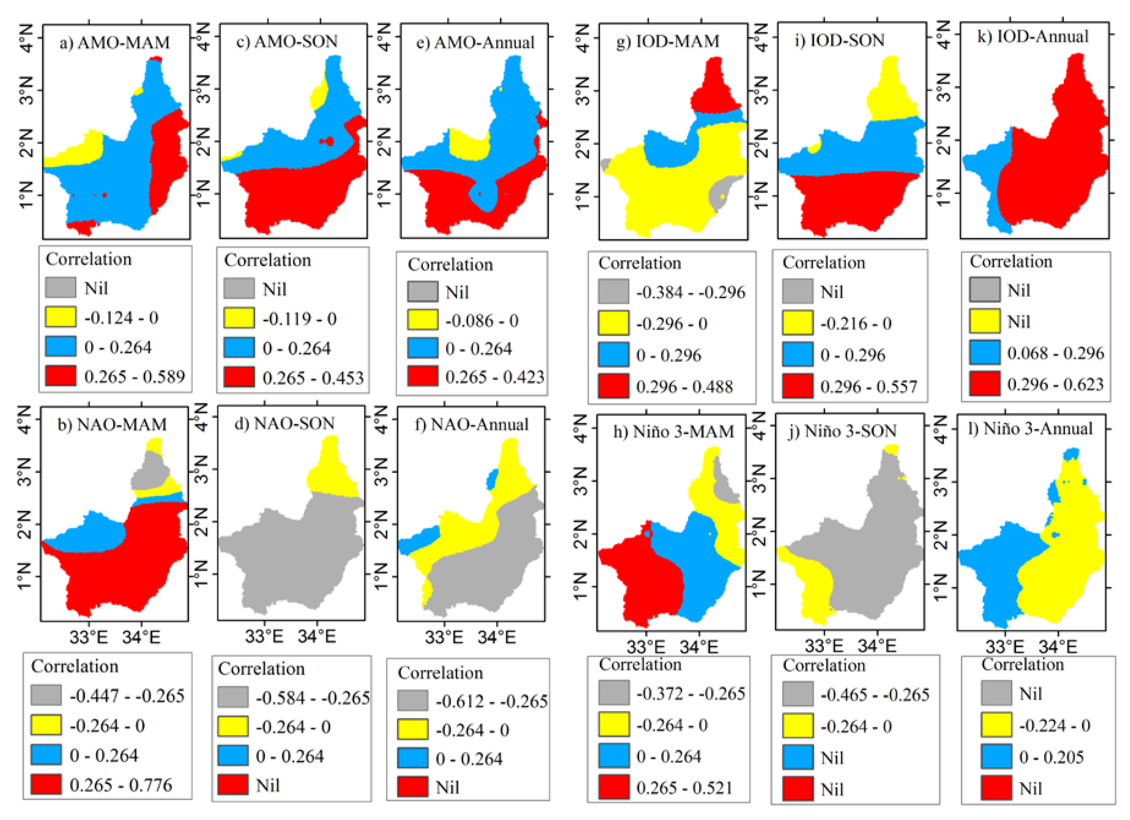
Figure 8 shows an insight on the linkage of the precipitation variation to the changes in the large-scale ocean–atmosphere conditions. The sample size of AMO, NAO or Niño 3 used in this study was 55. Using a two-tailed test, the critical value of the correlation between precipitation and AMO, NAO, and Niño 3 was 0.265. The critical correlation value for IOD (with sample size of 44) was 0.297. Precipitation across the LKB was generally found to be positively correlated with AMO (Figure 8a,c,e). Of the total variance in the SON and annual precipitation, 20.5% and 17.9% could be explained in terms of the variation in the AMO. The correlation between NAO and MAM precipitation was mainly positive (Figure 8b). The amount of precipitation variance that could be explained by the changes in NAO went up to 60.9%. However, SON and annual precipitation were found to be negatively correlated with NAO (Figure 8d,f). The amount of precipitation variance that could be explained by NAO for SON and annual precipitation (Figure 8d,f) was up to 34.1% and 37.5%, respectively. The H0 (no correlation) was rejected (p < 0.05) for the relation between NAO and precipitation in the Southern part (Figure 8b,d,f). The MAM precipitation (Figure 8g) across the LKB was generally positively correlated to the IOD except in the northeastern part. Both SON and annual precipitation (Figure 8i,k) was mainly positively correlated with IOD. The H0 (no correlation) was rejected (p < 0.05) for the relationship between IOD and the variation in the SON and annual precipitation in the southern and eastern parts, respectively. For annual time scale, the largest amount of precipitation variance (38.9%) was explained by the IOD. Niño 3 was positively and negative correlated with MAM precipitation in the western and northeastern parts, respectively (Figure 8h). However, SON precipitation was mainly negatively correlated with Niño 3 (Figure 8j). Niño 3 was positively and negatively correlated with annual precipitation in the western and eastern parts, respectively (Figure 8l). The H0 (no correlation) was rejected (p < 0.05) for the relation between Niño 3 and SON precipitation.
Figure 9 shows how the PET variability is linked to the large-scale ocean–atmosphere conditions. The critical correlation coefficients for Figure 9 were similar for the corresponding climate indices as given for Figure 8. For both seasonal and annual time scales, the correlation between MAM PET and AMO (Figure 9a) as well as NAO (Figure 9b) was mostly negative across the study area. The PET in the southern part was mainly positively correlated with IOD (Figure 9g,i,k). However, Niño 3 was mainly negatively correlated with MAM and annual PET (Figure 9h,l). Niño 3 was both positively and negatively correlated with western and eastern PET, respectively (Figure 9j). What is worth mentioning is that the results of the correlation analyses were less coherent for the PET (Figure 9a–l) than precipitation (Figure 8a–l).
4. Discussion
One of the findings from this study was that in most areas of the LKB (except in the eastern part of the LKB), precipitation from the rainy seasons as well as that from the annual time scale exhibited a decreasing (though insignificant p > 0.05) trend. The rate of this decrease was as low as −1.39, −0.752, and −0.078 mm/year for annual, MAM, and SON precipitation, respectively. Using ARC2 data from 1983 to 2012, Diem et al. [66] reported that precipitation in West-Central Uganda significantly decreased for multiple three-month periods centered on boreal summer. Furthermore, precipitation associated with the two rainy seasons decreased from 1983 to 2012 by 20% [66]. In our study, we found that at some of the locations where precipitation was decreasing, PET exhibited an increasing trend. Precipitation decrease and PET increase indicate a shift towards dry condition. If such trends are to continue into the future especially in the Equatorial region (where the LKB and Lake Victoria basin are located), the changes in the hydroclimate may affect the operations of water resources applications. For instance, the Karuma hydro power plant may not be able to generate power to its full capacity throughout the year due to erratic river flows stemming from the decreasing precipitation and increasing PET across the region. Furthermore, given that farming is the main occupation in this region, this finding shows the need to adopt good farming practices including mulching to improve soil moisture and fertility. New scientifically developed crop varieties, which are drought-resistant can be adopted by the smallholder farmers from this region.
Apart from the long-term trends, the precipitation and PET across the LKB were characterized by variability in terms of temporal occurrences of positive and negative subtrends. The results of variability showed that both seasonal and annual precipitation exhibited a decreasing subtrend in the 1990s. However, from the mid 2000 till the end of the data record (2015), precipitation was generally characterized by an increasing subtrend. Specifically, for the eastern part of the LKB (where Mt. Elgon is located), the change in precipitation from 1960 until the end of the data period (2015) was dominated by an increasing long-term trend. Between 1815 and 1959, landslides at the foot of Mt. Elgon occurred in 1818, 1900, 1918, 1922, 1927, 1933, 1942, and 1944 [67]. Between 1959 and 2009, landslides occurred at the foot of Mt. Elgon in 1960, 1967, 1970, 1997, and 1999 [67]. From 2010 to 2019 alone, landslides in Bududa occurred in March 2010, March 2011, June 2012, August 2013, October 2018, and December 2019 [21,68]. These records show that there were 8, 5, and 6 landslides over the periods 1818–1959 (142 years), 1960–2009 (50 years), and 2010–2019 (10 years), respectively. It is highly probable that the landslides have become more frequent recently than in the past due to the increasing precipitation trend in the eastern part of the LKB. These landslides claimed several lives and property as well as leading to the displacement of thousands of the local population. Due to the rapid population growth in the eastern part of the study area, there has been massive deforestation (for settlement, and cultivation) around the Mt. Elgon thereby rendering the area susceptible to landslides. Actually, “Deforestation and cultivation of steep concave slopes lower the threshold of slope stability, as they alter soil hydrological conditions within the slope elements by way of enhancing saturation, hence triggering debris flows” (Mugagga et al. [69]). If the increase in the precipitation in this region is to continue into the future, appropriate measures (such as preventive resettlement of the local population at the foot of Mt. Elgon, prevention of the encroachment of the gazetted forest reserve and national park in Mt. Elgon area, and restoration of the vegetation cover) should be implemented to avoid loss of lives and property due to landslides.
This study showed that the precipitation from the rainy seasons across the study area is correlated, to varying extents, with IOD, Niño 3, and AMO or NAO. Several studies assessed the correlation between the precipitation in the Equatorial region (where the LKB is located) and changes in SST or SLP from the Atlantic Ocean [2,66,70,71], and Indian Ocean [2,72,73]. Precipitation across the Equatorial region was also found linked to the El Niño Southern Oscillation (ENSO) [51,74,75,76,77,78]. Whereas our findings agree with results on teleconnections based on a number of previous studies, some differences were also noted especially with respect to the magnitudes (and directions, to some extent) of the correlation coefficients. Such differences could have been due to several reasons. Firstly, this study focused on MAM, SON, and annual precipitation while some other studies such as McHugh and Rogers [70] considered only the DJF season. Drivers of precipitation trends and variability may differ from one season to another [79]. Secondly, this study analyzed gridded CenTrends precipitation from 1961 to 2015. However other studies analyzed data from different sources considering various periods, for instance, CRU data from 1901 to 2015 [2], ARC2 over the period 1983–2012 [66], and observed precipitation at 37 stations with data covering period between 1900 and 2004 [51]. It is vital to note that, the drivers of precipitation or PET variability change in their strengths from one period to another. For instance, the ascending (or descending poles) of the Atlantic cell can be weak over one period and strong during another. Similarly, the descending or ascending poles of the Pacific cell can change in their strength among periods. Furthermore, the Indian Walter cell may be strong over one period but weak or moderate during another. This indicates that results of precipitation or PET variability attribution depend on the period selected for analysis. Another reason for some differences between our findings and results from other studies can be explained in terms of the methods used for analyses. Several methods were used in various studies to extract anomalies for attribution of precipitation variability. For instance, Onyutha and Willems [51] used the Quantile Perturbation Method, Indeje et al. [76] applied the Empirical Orthogonal Functions, and Onyutha [2] (like in this study) analyzed variability in terms of the occurrences of positive and negative subtrends over time. Variability in the same precipitation series can temporally differ among the methods applied. This means that results of correlation between climate indices and precipitation anomalies can depend on the selected method applied for deriving the variability. Despite the above reasons, this study established that the magnitude (and sign) of the correlation depends on the chosen climate index or location where the precipitation is selected for analysis.
With respect to the annual time scale, the largest amount of variance in precipitation (38.9%) and PET (41.2%) was found to be explained by the IOD. The second largest amount of variance in precipitation (17.9%) and PET (21.9%) was found to be explained by the AMO and NAO, respectively. However, the IOD processes or linkages to AMO or NAO could not explain all the precipitation variance. Other factors which could be controlling the precipitation and PET variability across the study area include the influences from a number of topographical features such as lakes (Kyoga, Victoria, and Albert), and high mountains (Mt. Elgon, Mt. Rwenzori, and Mt. Kenya) [80]. Generally, knowledge of the driver of precipitation and/or PET variability is important in prediction of an upcoming epoch of wet or dry condition. Eventually, there can be a careful planning of predictive adaptation to the impacts of climate variability on hydrometeorology.
5. Conclusions
This study analyzed changes in precipitation and PET across the LKB. This study made use of gridded CenTrends monthly precipitation dataset [30] and PET derived from the PGF-based Tmax and Tmin series [4]. The changes in precipitation and PET were in terms of long-term trends and variability based on the temporal variation of subtrends. Possible linkages of precipitation and PET variability to large scale ocean–atmospheric interactions were assessed. Both seasonal and annual precipitation from 1960 to 2015 exhibited an insignificant (p > 0.05) decrease in most parts of the LKB. However, at some of the locations, PET exhibited an increasing (though insignificant p > 0.05) trend. Such precipitation decrease accompanied by an increasing PET can negatively affect river flow thereby affecting some of the water resources applications in the study area.
Both seasonal and annual precipitation exhibited decreasing subtrends in the 1960s and 1990s. However, from the mid 2000 until the mid-2010s (or end of the data record or 2015), precipitation was generally characterized by an increasing subtrend. For the eastern part of the LKB (where Mt. Elgon is located), the change in precipitation from 1960 until the end of the data period (2015) was dominated by an increasing long-term trend. This increasing precipitation is a critical cause of the several recent landslides in Bududa located in the eastern part of the LKB. Human activities such as massive deforestation and overgrazing exacerbate the occurrences of precipitation-induced landslides. With respect to the annual time scale, the largest amount of variance in precipitation (38.9%) and PET (41.2%) was found to be explained by the IOD. The second largest amount of variance in precipitation (17.9%) and PET (21.9%) was found to be explained by the AMO and NAO, respectively. In terms of the strength of the correlation between precipitation and climate indices, some differences were noted between our findings and results from other or previous studies. Such slight discrepancies were mainly due to the differences (among studies) in (i) the methods for computing variability, (ii) the periods selected for analyses, and (iii) the sources of data considered for studies. Nevertheless, the findings from this study are important for predictive adaptation to the impacts of climate variability on hydrometeorology, and agriculture in the study area.
Even if the CenTrends data were derived by interpolation of station-based weather data, still some minor validation was conducted at two locations within the study area considering the period 1961–2000. The mismatch between the long-term monthly mean from the observed and CenTrends precipitation was minimal. However, there were some differences in the long-term trends from the observed and CenTrends. Importantly, results showed close agreement between the observed and CenTrends precipitation variability from 1961 until the late 1970s. However, from 1980 until 2000, there was some mismatch between observed and CenTrends precipitation. This could be due to the consideration of fewer precipitation stations before than after 1980 in the derivation of precipitation interpolation products over the LKB. This suggests the need for an update of the CenTrends v1.0 data to incorporate observations (if available) at more stations from Uganda to reflect the precipitation variability especially from around 2000 to the present.
Comparison of PET based on observed and PGF temperature was made in terms of long-term monthly mean, trends and variability. The PGF data did not adequately reproduce the bimodal pattern in observed temperature. For each month, the PGF underestimated observed Tmax by about 50%. Eventually, the PGF data underestimated the observed differences between Tmax and Tmin, an aspect that comprises of a key component in the computation of PET. Trends or variability in observed and PGF-based data tended to differ to some extent across the seasonal and annual time scales. This indicated the need for improving the quality of PGF data in reproducing observed climatology of the Equatorial region and/or East Africa.
Variation in river flow can be influenced by both climate variability and human factors [81]. Therefore, it is recommended that future research to supplement the findings of this study should consider an assessment of the impact of land use on the variation in PET and lake level, and investigating the impacts of climate variability and climate change on hydrometeorology of the LKB.
Author Contributions
All authors were involved in the conception of the study. C.O. and G.A were further involved in data acquisition, analyses, interpretation, drafting manuscript and making necessary revision. C.O. and J.N. were supervisors to G.A. when conducting this study. All authors have read and agreed to the published version of the manuscript.
Funding
This research received no external funding.
Acknowledgments
The authors acknowledge that the CentTrends [30] and Princeton Global Forcing [4] data were used in this study. The authors acknowledge that this paper was partly based on a study by Grace Acayo [82] under the supervision of Charles Onyutha, and Jacob Nyende. The authors are grateful to the three anonymous reviewers for their meticulous comments and suggestions that greatly shaped the contents and quality of this paper.
Conflicts of Interest
The authors declare no conflict of interest.
Appendix A. Further Information on Trend Significance
Figure A1.
Statistical trend statistic Z for (a–c) precipitation and (d–f) PET of (a,d) MAM, (b,e) SON, and (c,f) annual time scales.
Figure A1.
Statistical trend statistic Z for (a–c) precipitation and (d–f) PET of (a,d) MAM, (b,e) SON, and (c,f) annual time scales.

References
- Brown, E.; Sutcliffe, J.V. The water balance of Lake Kyoga, Uganda. Hydrol. Sci. J. 2013, 58, 342–353. [Google Scholar] [CrossRef] [Green Version]
- Onyutha, C. Trends and variability in African long-term precipitation. Stoch. Environ. Res. Risk Assess 2018, 32, 2721–2739. [Google Scholar] [CrossRef]
- Southwell, T.M. Groundwater – surface water interactions of papyrus wetlands in the Lake Kyoga basin of Uganda. In Dissertation for Masters of Natural Resource Management; Norwegian University of Life Science: Ås, Norway, 2016. [Google Scholar]
- Sheffield, J.; Goteti, G.; Wood, E.F. Development of a 50-year high-resolution global dataset of meteorological forcings for land surface modeling. J. Clim. 2006, 19, 3088–3111. [Google Scholar] [CrossRef] [Green Version]
- Adler, R.F.; Huffman, G.F.; Chang, A.; Ferraro, R.; Xie, P.-P.; Janowiak, J.; Rudolf, B.; Schneider, U.; Curtis, S.; Bolvin, D.; et al. Version-2 global precipitation climatology project (GPCP) monthly precipitation analysis (1979-present). J. Hydrometeorol. 2003, 4, 1147–1167. [Google Scholar] [CrossRef]
- Harris, I.; Jones, P.D.; Osborn, T.J.; Lister, D.H. Updated high resolution grids of monthly climatic observations–the CRU TS3.10 dataset. Int. J. Clim. 2014, 34, 623–642. [Google Scholar] [CrossRef] [Green Version]
- Novella, N.S.; Thiaw, W.M. African rainfall climatology version 2 for famine early warning systems. J. Appl. Meteorol. Climatol. 2013, 52, 588–606. [Google Scholar] [CrossRef]
- Huffman, G.J.; Bolvin, D.T.; Nelkin, E.J.; Wolff, D.B. The TRMM multisatellite precipitation analysis (TMPA): Quasi-global, multiyear, combined-sensor precipitation estimates at fine scales. J. Hydrometeorol. 2007, 8, 38–55. [Google Scholar] [CrossRef]
- NCEP. NCEP Climate Forecast System Reanalysis (CFSR). Available online: http://rda.ucar.edu/ (accessed on 28 March 2020).
- Hoell, A.; Shukla, S.; Barlow, M.; Cannon, F.; Kelley, C.; Funk, C. The forcing of monthly precipitation variability over Southwest Asia during the Boreal Cold Season. J. Clim. 2015, 28, 7038–7056. [Google Scholar] [CrossRef]
- Onyutha, C. Geospatial trends and decadal anomalies in extreme rainfall over Uganda, East Africa. Adv. Meteorol. 2016, 2016, 1–15. [Google Scholar] [CrossRef] [Green Version]
- Zeng, R.; Cai, X. Climatic and terrestrial storage control on evapotranspiration temporal variability: Analysis of river basins around the world. Geophys. Res. Lett. 2016, 43, 185–195. [Google Scholar] [CrossRef]
- Onyutha, C. On rigorous drought assessment using daily time scale: Non-stationary frequency analyses, revisited concepts, and a new method to yield non-parametric indices. Hydrology 2017, 4, 48. [Google Scholar] [CrossRef] [Green Version]
- Glenn, E.P.; Huete, A.R.; Nagler, P.L.; Hirschboeck, K.K.; Brown, P. Integrating remote sensing and ground methods to estimate evapotranspiration. Crit Rev. Plant. Sci. 2007, 26, 139–168. [Google Scholar] [CrossRef]
- Vinukollu, R.K.; Wood, E.F.; Ferguson, C.R.; Fisher, J.B. Global estimates of evapotranspiration for climate studies using multi-sensor remote sensing data: Evaluation of three process-based approaches. Remote Sens. Environ. 2011, 115, 801–823. [Google Scholar] [CrossRef]
- Gentilucci, M.; Barbieri, M.; Burt, P. Climate and territorial suitability for the Vineyards developed using GIS techniques. In Exploring the Nexus of Geoecology, Geography, Geoarcheology and Geotourism: Advances and Applications for Sustainable Development in Environmental Sciences and Agroforestry Research. CAJG 2018. Advances in Science, Technology & Innovation (IEREK Interdisciplinary Series for Sustainable Development); Chenchouni, H., Errami, E., Rocha, F., Sabato, L., Eds.; Springer: Cham, Switzerland, 2019. [Google Scholar]
- Alemu, H.; Senay, G.B.; Kaptue, A.T.; Kovalskyy, V. Evapotranspiration variability and its association with vegetation dynamics in the Nile Basin, 2002–2011. Remote Sens. 2014, 6, 5885–5908. [Google Scholar] [CrossRef] [Green Version]
- Liou, Y.-A.; Kar, S.K. Evapotranspiration estimation with remote sensing and various surface energy balance algorithms—A review. Energies 2014, 7, 2821–2849. [Google Scholar] [CrossRef] [Green Version]
- Bashir, M.; Tanakamaru, H.; Tada, A. Remote Sensing-based Estimates of Evapotranspiration for Managing Scarce Water Resources in the Gezira Scheme, Sudan. In From Headwaters to the Ocean, Hydrological Change and Water Management; Taniguchi, M., Burnett, W.C., Fukushima, Y., Haigh, M., Umezawa, Y., Eds.; CRC Press: Boca Raton, FL, USA, 2008; pp. 381–386. [Google Scholar]
- Nsubuga, F.W.N.; Botai, J.O.; Olwoch, J.M.; deW Rautenbach, C.J.; Kalumba, A.M.; Tsela, P.; Adeola, A.M.; Sentongo, A.A.; Mearns, K.F. Detecting changes in surface water area of Lake Kyoga sub-basin using remotely sensed imagery in a changing climate. Appl. Clim. 2017, 127, 327–337. [Google Scholar] [CrossRef] [Green Version]
- Reliefweb. Several killed as landslides hit Bududa, Sironko. Available online: https://reliefweb.int/report/uganda/several-killed-landslides-hit-bududa-sironko (accessed on 20 December 2019).
- Twongo, T. The Fisheries and Environment of Kyoga Lakes; Fisheries Resources Research Institute FIRRI: Jinja, Uganda, 2001. [Google Scholar]
- Shahin, M. Hydrology of the Nile Basin, Developments in Water Science, 21st ed.; Elsevier: Amsterdam, The Netherlands, 1985. [Google Scholar]
- FAO. Irrigation Potential in Africa: A Basin Approach, FAO Land and Water Bulletin No. 4; FAO: Rome, Italy, 1997. [Google Scholar]
- Onyutha, C.; Willems, P. Investigation of flow-rainfall co-variation for catchments selected based on the two main sources of River Nile. Stoch. Environ. Res. Risk Assess. 2018, 32, 623–641. [Google Scholar] [CrossRef]
- Jarvis, A.; Reuter, H.I.; Nelson, A.; Guevara, E. Hole-filled seamless SRTM data V4, International Centre for Tropical Agriculture (CIAT). Available online: http://srtm.csi.cgiar.org (accessed on 20 December 2019).
- Reuter, H.I.; Nelson, A.; Jarvis, A. An evaluation of void filling interpolation methods for SRTM data. Int. J. Geogr. Inform. Sci. 2007, 21, 983–1008. [Google Scholar] [CrossRef]
- Kottek, M.; Grieser, J.; Beck, C.; Rudolf, B.; Rubel, F. World map of the Köppen-Geiger climate classification updated. Meteorol. Zeitschrift 2006, 15, 259–263. [Google Scholar] [CrossRef]
- Peel, M.C.; Finlayson, B.L.; Mcmahon, T.A. Updated world map of the Köppen-Geiger climate classification. Hydrol. Earth Syst. Sci. 2007, 11, 1633–1644. [Google Scholar] [CrossRef] [Green Version]
- Funk, C.; Nicholson, S.E.; Landsfeld, M.; Klotter, D.; PETerson, P.; Harrison, L. The Centennial Trends Greater Horn of Africa precipitation dataset. Sci. Data 2015, 2, 1–17. [Google Scholar] [CrossRef]
- Allen, R.G.; Pereira, L.S.; Raes, D.; Smith, M. Crop Evapotranspiration—Guidelines for Computing Crop Water Requirements—FAO Irrigation and Drainage Paper 56; FAO—Food and Agriculture Organization of the United Nations: Rome, Italy, 1998. [Google Scholar]
- Makkink, G.F. Testing the Penman formula by means of lysimeters. J. Inst. Water. Eng. 1957, 11, 277–288. [Google Scholar]
- Hargreaves, G.H.; Samni, Z.A. Estimation of potential evapotranspiration. Proc. Am. Soc. Civ. Eng. 1982, 108, 223–230. [Google Scholar]
- Hargreaves, G.H.; Samni, Z.A. Reference crop evapotranspiration from temperature. Trans. Am. Soc. Agric. Eng. 1985, 1, 96–99. [Google Scholar] [CrossRef]
- Blaney, H.F.; Criddle, W.D. Determining Water Requirements in Irrigated Areas from Climatological Irrigation Data; U.S. Soil Conservation Service: Washington, DC, USA, 1950; Volume 48.
- Priestley, C.H.B.; Taylor, R.J. On the assessment of the surface heat flux and evaporation using large-scale parameters. Mon. Weather. Rev. 1972, 100, 81–92. [Google Scholar] [CrossRef]
- Rohwer, C. Evaporation from free water surface. Usda Tech. Null 1931, 217, 1–96. [Google Scholar]
- Tabari, H.; Grismer, M.E.; Trajkovic, S. Comparative analysis of 31 reference evapotranspiration methods under humid conditions. Irrig. Sci. 2013, 31, 107–117. [Google Scholar] [CrossRef]
- Lang, D.; Zheng, J.; Shi, J.; Liao, F.; Ma, X.; Wang, W.; Zhang, M. A comparative study of potential evapotranspiration estimation by eight methods with FAO Penman—Monteith method in southwestern China. Water 2017, 9, 734. [Google Scholar] [CrossRef] [Green Version]
- Liu, W.; Liu, L. Analysis of dry/wet variations in the Poyang Lake basin using standardized precipitation evapotranspiration index based on two potential evapotranspiration algorithms. Water 2019, 11, 1380. [Google Scholar] [CrossRef] [Green Version]
- Pan, S.; Xu, Y.P.; Xuan, W.; Gu, H.; Bai, Z. Appropriateness of potential evapotranspiration models for climate change impact analysis in Yarlung Zangbo River basin, China. Atmosphere 2019, 10, 453. [Google Scholar] [CrossRef] [Green Version]
- Chuanyan, Z.; Zhongren, N.; Zhaodong, F. GIS-assisted spatially distributed modeling of the potential evapotranspiration in semi-arid climate of the Chinese Loess Plateau. J. Arid. Environ. 2004, 58, 387–403. [Google Scholar] [CrossRef]
- Behnke, J.J.; Maxey, G.B. An empirical method for estimating monthly potential evapotranspiration in Nevada. J. Hydrol. 1969, 8, 418–430. [Google Scholar] [CrossRef]
- Hurrell, J.W. Decadal trends in the North Atlantic Oscillation and relationships to regional temperature and precipitation. Science 1995, 269, 676–679. [Google Scholar] [CrossRef] [PubMed] [Green Version]
- Jones, P.D.; Jónsson, T.; Wheeler, D. Extension to the North Atlantic Oscillation using early instrumental pressure observations from Gibraltar and South-West Iceland. Int. J. Clim. 1997, 17, 1433–1450. [Google Scholar] [CrossRef]
- Van Oldenborgh, G.J.; te Raa, L.A.; Dijkstra, H.A.; Philip, S.Y. Frequency or amplitude dependent effects of the Atlantic meridional overturning on the tropical Pacific Ocean. Ocean. Sci. 2009, 5, 293–301. [Google Scholar] [CrossRef] [Green Version]
- Enfield, D.B.; Mestas-Nunez, A.M.; Trimble, P.J. The Atlantic multidecadal oscillation and it’s relation to rainfall and river flows in the continental U.S. Geophys. Res. Lett. 2001, 28, 2077–2080. [Google Scholar] [CrossRef] [Green Version]
- Rayner, N.A.; Parker, D.E.; Horton, E.B.; Folland, C.K.; Alexander, L.V.; Rowell, D.P.; Kent, E.C.; Kaplan, A. Global analyses of sea surface temperature, sea ice, and night marine air temperature since the late nineteenth century. J. Geophys. Res. 2003, 108, 4407. [Google Scholar] [CrossRef]
- Trenberth, K.E. The Definition of El Niño. B Am. Meteorol. Soc. 1997, 78, 2771–2777. [Google Scholar] [CrossRef] [Green Version]
- Saji, N.H.; Goswami, B.N.; Vinayachandran, P.N.; Yamagata, T. A dipole mode in the tropical Indian Ocean. Nature 1999, 401, 360–363. [Google Scholar] [CrossRef]
- Onyutha, C.; Willems, P. Spatial and temporal variability of rainfall in the Nile Basin. Hydrol. Earth Sys. Sci. 2015, 19, 2227–2246. [Google Scholar] [CrossRef] [Green Version]
- Theil, H. A rank-invariant method of linear and polynomial regression analysis. Nederl. Akad. Wetench. Ser. A 1950, 53, 386–392. [Google Scholar]
- Sen, P.K. Estimates of the regression coefficient based on Kendall’s tau. J. Am. Stat. Assoc. 1968, 63, 1379–1389. [Google Scholar] [CrossRef]
- Mann, H.B. Nonparametric tests against trend. Econometrica 1945, 13, 245–259. [Google Scholar] [CrossRef]
- Kendall, M.G. Rank Correlation Methods, 4th ed; Charles Griffin: London, UK, 1975. [Google Scholar]
- Spearman, C. The proof and measurement of association between two things. Am. J. Psychol. 1904, 15, 72–101. [Google Scholar] [CrossRef]
- Lehmann, E.L. Nonparametrics, Statistical Methods Based on Ranks; Holden-Day Inc.: Oakland, CA, USA, 1975. [Google Scholar]
- Sneyers, R. On the Statistical Analysis of Series of Observations Technical Note no. 143, WMO no. 415; Secretariat of the World Meteorological Organization: Geneva, Switzerland, 1990. [Google Scholar]
- Onyutha, C. Identification of sub-trends from hydro-meteorological series. Stoch Environ. Res. Risk Assess 2016, 30, 189–205. [Google Scholar] [CrossRef]
- Onyutha, C. Statistical analyses of potential evapotranspiration changes over the period 1930–2012 in the Nile River riparian countries. Agric. For. Meteorol. 2016, 226, 80–95. [Google Scholar] [CrossRef]
- Onyutha, C. Statistical Uncertainty in Hydrometeorological Trend Analyses. Adv. Meteorol. 2016, 2016, 26. [Google Scholar] [CrossRef] [Green Version]
- Pirnia, A.; Golshan, M.; Darabi, H.; Adamowski, J.F.; Rozbeh, S. Using the Mann–Kendall test and double mass curve method to explore stream flow changes in response to climate and human activities. J. Water Clim. Chang. 2018, 10, 725–742. [Google Scholar] [CrossRef]
- Tang, L.; Zhang, Y. Considering abrupt change in rainfall for flood season division: A case study of the Zhangjia Zhuang reservoir, based on a new model. Water 2018, 10, 1152. [Google Scholar] [CrossRef] [Green Version]
- Vido, J.; Nalevanková, P.; Valach, J.; Šustek, Z.; Tadesse, T. Drought Analyses of the Horné Požitavie Region (Slovakia) in the Period 1966–2013. Adv. Meteorol. 2019, 2019, 1–10. [Google Scholar] [CrossRef]
- Cengiz, T.M.; Tabari, H.; Onyutha, C.; Kisi, O. Combined use of graphical and statistical approaches for analyzing historical precipitation changes in the Black Sea region of Turkey. Water 2020, 12, 705. [Google Scholar] [CrossRef] [Green Version]
- Diem, J.E.; Ryan, S.J.; Hartter, J.; Palace, M.W. Satellite-based rainfall data reveal a recent drying trend in central equatorial Africa. Clim. Change 2014, 126, 263–272. [Google Scholar] [CrossRef]
- UNCU. Landslides in Uganda. Retrieved online from the website of the Uganda National Commission for UNESCO (UNCU). 2019. Available online: http://unesco-uganda.ug/wp-content/uploads/2019/02/LandSlides-In-Uganda.pdf (accessed on 1 April 2020).
- ACAPS. Uganda: Flooding and landslides in Bududa. Available online: https://www.acaps.org/sites/acaps/files/products/files/20181018_acaps_start_briefing_note_uganda_flooding_and_landslides_in_bududa.pdf (accessed on 20 December 2019).
- Mugagga, F.; Kakembo, V.; Buyinza, M. Land use changes on the slopes of Mount Elgon and the implications for the occurrence of landslides. Catena 2012, 90, 39–46. [Google Scholar] [CrossRef]
- McHugh, M.J.; Rogers, J.C. North Atlantic oscillation influence on precipitation variability around the southeast African convergence zone. J. Clim. 2001, 14, 3631–3642. [Google Scholar] [CrossRef]
- Zhang, R.; Delworth, T.L. Impact of Atlantic multidecadal oscillations on India/Sahel rainfall and Atlantic hurricanes. Geophys. Res. Lett. 2006, 33. [Google Scholar] [CrossRef] [Green Version]
- Liebmann, B.; Hoerling, M.P.; Funk, C.; Bladé, I.; Dole, R.M.; Allured, D.; Quan, X.; Pegion, P.; Eischeid, J.K. Understanding recent eastern Horn of Africa rainfall variability and change. J. Clim. 2014, 27, 8630–8645. [Google Scholar] [CrossRef]
- Bergonzini, L.; Richard, Y.; PETit, L.; Camberlin, P. Zonal circulations over the Indian and Pacific oceans and the level of Lakes Victoria and Tanganyika. Int. J. Climatol. 2004, 24, 1613–1624. [Google Scholar] [CrossRef]
- Nicholson, S.E. A review of climate dynamics and climate variability in Eastern Africa. In The Limnology, Climatology and Paleoclimatology of the East African Lakes; Johnson, T.C., Odada, E.O., Eds.; Gordon and Breach: Amsterdam, The Netherlands, 1996; pp. 25–56. [Google Scholar]
- Phillips, J.; McIntyre, B. ENSO and interannual rainfall variability in Uganda: Implications for agricultural management. Int J. Climatol. 2000, 20, 171–182. [Google Scholar] [CrossRef]
- Indeje, M.; Semazzi, H.F.M.; Ogallo, L.J. ENSO signals in East African rainfall seasons. Int. J. Climatol. 2000, 20, 19–46. [Google Scholar] [CrossRef]
- Schreck, C.J.; Semazzi, F.H.M. Variability of the recent climate of Eastern Africa. Int. J. Climatol. 2004, 24, 681–701. [Google Scholar] [CrossRef]
- Williams, A.; Funk, C. A westward extension of the warm pool leads to a westward extension of the Walker circulation, drying Eastern Africa. Clim. Dyn. 2011, 37, 2417–2435. [Google Scholar] [CrossRef] [Green Version]
- Onyutha, C.; Tabari, H.; Taye, M.T.; Nyandwaro, G.N.; Willems, P. Analyses of rainfall trends in the Nile River Basin. J. Hydro Environ. Res. 2016, 13, 36–51. [Google Scholar] [CrossRef]
- Onyutha, C.; Tabari, H.; Rutkowska, A.; Nyeko-Ogiramoi, P.; Willems, P. Comparison of different statistical downscaling methods for climate change rainfall projections over the Lake Victoria basin considering CMIP3 and CMIP5. J. Hydro Environ. Res. 2016, 12, 31–45. [Google Scholar] [CrossRef]
- Pirnia, P.; Darabi, H.; Choubin, B.; Omidvar, E.; Onyutha, C.; Haghighi, A.T. Contribution of climatic variability and human activities to stream flow changes in the Haraz River basin, northern Iran. J. Hydro Environ. Res. 2019, 25, 12–24. [Google Scholar] [CrossRef]
- Acayo, G. Analyses of Multi-Decadal Variability and Trends in Precipitation and Potential Evapotranspiration across the Lake Kyoga Basin. In Dissertation for MSc in Water and Sanitation Engineering; Department of Civil and Building Engineering, Kyambogo University: Kyambogo, Uganda, 2020. [Google Scholar]
Figure 1.
The Lake Kyoga Basin.

Figure 2.
Mean of long-term monthly precipitation at selected locations in the Lake Kyoga Basin (LKB).
Figure 2.
Mean of long-term monthly precipitation at selected locations in the Lake Kyoga Basin (LKB).

Figure 3.
Mean of long-term monthly PET at selected locations in the LKB.

Figure 4.
Time series plots of annual (a,b) precipitation, (c) Tmax, and (d) PET. The legend of chart (b) and (d) is similar to that of (a) and (c), respectively. “Obs” stands for observed (a,b) precipitation, (c) Tmax, and (d) PET.
Figure 4.
Time series plots of annual (a,b) precipitation, (c) Tmax, and (d) PET. The legend of chart (b) and (d) is similar to that of (a) and (c), respectively. “Obs” stands for observed (a,b) precipitation, (c) Tmax, and (d) PET.

Figure 5.
Trends slopes in (a–c) precipitation and (d–f) PET of (a,d) March–April–May (MAM), (b,e) September–October–November (SON), and (d,f) annual scales.
Figure 5.
Trends slopes in (a–c) precipitation and (d–f) PET of (a,d) March–April–May (MAM), (b,e) September–October–November (SON), and (d,f) annual scales.

Figure 6.
Variability in precipitation at (a,b) Station 1, (d–f) Station 2, and PET at (g–i) Station B based on (a,d,g) MAM, (b,e,h) SON, and (c,f,i) annual time scales. In each chart, “Obs” means observed variable, and the dotted horizontal lines denote the 95% CI limits.
Figure 6.
Variability in precipitation at (a,b) Station 1, (d–f) Station 2, and PET at (g–i) Station B based on (a,d,g) MAM, (b,e,h) SON, and (c,f,i) annual time scales. In each chart, “Obs” means observed variable, and the dotted horizontal lines denote the 95% CI limits.

Figure 7.
Variability in (a–d) MAM, (e–h) SON, and (i–l) annual precipitation and PET for the (a,e,i) southern, (b,f,j) northern, (c,g,k) eastern, and (d,h,l) western parts of the LKB. All charts share the same legend as in (e) and the dotted horizontal lines denote the 95% CI limits.
Figure 7.
Variability in (a–d) MAM, (e–h) SON, and (i–l) annual precipitation and PET for the (a,e,i) southern, (b,f,j) northern, (c,g,k) eastern, and (d,h,l) western parts of the LKB. All charts share the same legend as in (e) and the dotted horizontal lines denote the 95% CI limits.

Figure 8.
Correlation between precipitation and climate indices considering (a,b,g–h) MAM, (c,d,i–j) SON, and (e–f,k–l) annual time scales.
Figure 8.
Correlation between precipitation and climate indices considering (a,b,g–h) MAM, (c,d,i–j) SON, and (e–f,k–l) annual time scales.

Figure 9.
Correlation between PET and climate indices considering ((a,b,g–h)) MAM, (c,d,i–j) SON, and (e–f,k–l) annual time scales.
Figure 9.
Correlation between PET and climate indices considering ((a,b,g–h)) MAM, (c,d,i–j) SON, and (e–f,k–l) annual time scales.


Table 1.
Correlation between climate indices and precipitation or PET.
| Station | Scale | NAO | IOD | Niño 3 | AMO | NAO | IOD | Niño 3 | AMO |
|---|---|---|---|---|---|---|---|---|---|
| 1 | Observed precipitation | CenTrends precipitation | |||||||
| MAM | −0.20 | 0.48 * | −0.03 | 0.06 | −0.06 | 0.38 * | −0.23 | 0.45 * | |
| SON | 0.25 | −0.29 | −0.04 | 0.42 * | −0.36 * | 0.19 | −0.65 * | 0.57 * | |
| Annual | −0.46 * | 0.46 * | 0.19 | 0.21 | −0.49 * | 0.63 * | −0.27 | 0.53 * | |
| 2 | Observed precipitation | CenTrends precipitation | |||||||
| MAM | −0.50 * | 0.46 * | 0.22 | 0.08 | 0.32 * | 0.03 | 0.11 | 0.32 * | |
| SON | −0.04 | 0.12 | −0.35 * | 0.33 * | −0.67 * | 0.41 * | −0.38 * | 0.68 * | |
| Annual | −0.48 * | 0.61 * | 0.16 | 0.17 | −0.44 * | 0.73 * | −0.17 | 0.67 * | |
| B | PET from observed temperature | PET based on PGF temperature | |||||||
| MAM | −0.23 | −0.41 | 0.48 * | 0.19 | −0.21 | 0.69 * | −0.31 | −0.48 * | |
| SON | −0.33 | 0.26 | −0.67 * | −0.28 | −0.53 * | 0.12 | 0.55 * | 0.77 * | |
| Annual | 0.10 | −0.21 | 0.23 | 0.70 * | −0.74 * | −0.36 | −0.07 | 0.25 | |
Note: * means H0 (no correlation) was rejected at α = 0.05.
© 2020 by the authors. Licensee MDPI, Basel, Switzerland. This article is an open access article distributed under the terms and conditions of the Creative Commons Attribution (CC BY) license (http://creativecommons.org/licenses/by/4.0/).
Share and Cite
MDPI and ACS Style
Onyutha, C.; Acayo, G.; Nyende, J. Analyses of Precipitation and Evapotranspiration Changes across the Lake Kyoga Basin in East Africa. Water 2020, 12, 1134. https://doi.org/10.3390/w12041134
AMA Style
Onyutha C, Acayo G, Nyende J. Analyses of Precipitation and Evapotranspiration Changes across the Lake Kyoga Basin in East Africa. Water. 2020; 12(4):1134. https://doi.org/10.3390/w12041134
Chicago/Turabian StyleOnyutha, Charles, Grace Acayo, and Jacob Nyende. 2020. "Analyses of Precipitation and Evapotranspiration Changes across the Lake Kyoga Basin in East Africa" Water 12, no. 4: 1134. https://doi.org/10.3390/w12041134
Note that from the first issue of 2016, this journal uses article numbers instead of page numbers. See further details here.