Evaluation of the Methodology to Assess the Influence of Hydraulic Characteristics on Habitat Quality

Abstract

The article aims at assessing the impact of hydraulic characteristics on the habitat quality of mountain and piedmont watercourses. The solution results from the Riverine Habitat Simulation model, where the quality of the aquatic habitat is represented by the weighted usable area (WUA), which is determined using brown trout as the bioindicator. Flow velocity and water depth are basic abiotic characteristics that determine the ratio of suitability of the instream habitat represented by the weighted usable area. The influence of these parameters on the objective evaluation of the habitat quality is the essence of the paper. The measurements were carried out during the summer period at minimum discharges for 17 mountain and piedmont streams in Slovakia. Three methods for assessing the habitat quality were tested, and differences in the results were found to be significant. The evaluation shows the optimum design methods for calculating the weighted usable area.

1. Introduction

River systems are significantly related to the development of relief when creating a river network and to the riverbed morphology [1]. An aquatic ecosystem in a good condition can serve numerous of functions, such as production, regulation, and flood protection, as well as a positive cultural impact [2].

Therefore, it is important to know the impact of the hydromorphological characteristics of the stream on the aquatic ecosystem [3,4]. Abiotic characteristics, together with habitat quality, form the basis for assessing the habitat availability [5,6]. The set of these relationships is the basis for a comprehensive environmental assessment. A variety of landscape-planning methods and landscape ecology methods are available to predict and assess these impacts [7,8,9,10].

Today, there are models that specifically confirm the challenge for fish river communities and indicate a strong pressure caused by the climate change and human activity. Well-known are mainly models based on the instream flow incremental methodology (IFIM), which belong to the decision-making methods (the results are discussed in the decision-making committee—a wider range of experts). The IFIM models are composed of a library of linked analytical procedures that describe the spatial and temporal features of a habitat, resulting from a given river regulation alternative—components can be combined to fit specific needs [11]. These models predict a severe decline in the number and biomass of fish due to climate change. Despite the strong evolutionary adaptations of individual species, the decreasing rate is higher in the scenario of the combination of warming and the flow reduction, which inevitably leads to a high probability of population extinction [12]. The evaluation of the impact of climate change on the quality of the aquatic habitat on the Drietomica stream (piedmont) shows that, during the 2071–2100 horizon, the minimum flow rates will fall by 50% in the summer [13]. Such changes can also be expected in other mountain and piedmont streams of the Carpathian system. This change will have a significant impact on the aquatic habitat. Therefore, it would be appropriate to carry out the restoration and rehabilitation of streams, which would be based on the flow rate forecast.

Fishes as bioindicators have been selected because of their suitability for assessing the ecological integrity of rivers, for their sensitivity to changes in river habitats, occurrence, longevity, and mobility [11,14,15]. Changing the riverbed morphology and, hence, faster water heating is a significant threat to fish, as they are ectothermic animals [16]. For this reason, fish are highly physiologically linked to local climate conditions, which can eliminate their resilience and tolerance to climate and anthropological changes [17]. According to [18], there are several methods to assess the consequences of changes in watercourses, but a key aspect is to assess and identify the relationships between ichthyofauna and physical components. It is therefore important to improve and simplify the methodology for assessing the geomorphology of the current state of rivers and its impact on the habitat preferences of particular fish species on the basis of clear quantitative and consistent criteria [19] and making the corrective or mitigate measures available to the general public. An interdisciplinary approach that has led to the emergence of a new scientific discipline, ecohydraulics, is needed to assess such a complex system. Ecohydraulics is a subdiscipline of ecohydrology, including hydraulics and geomorphology and their impact on the aquatic ecosystem. This study is within the intentions of ecohydraulics, which represents adequate and interdisciplinary modeling and the assessing of the current state of rivers and the design of restoration measures and techniques to mitigate anthropogenic impacts [20]. The Riverine HABitat SIMulation (RHABSIM) model that fits within the ecohydraulic principles was used to gather the results presented in this study.

Further research [15] compared the differences in geomorphology between natural and regulated streams and their impact on biota, since natural channels differ from prismatic ones by their rich variability of the cross-section (XS) and longitudinal channel profiles. Typical consequences of geometrical river regulations for the biota are the reduction of original instream habitat complexities and habitat availabilities in increasingly uniform riverbeds [21]. It is the morphology of such regulated rivers that is the main reason for the loss of biota and the degradation of the value of the river. It is important to propose remedies based on objective information [22]. Fish as bioindicators can be considered as a reliable source of such information.

When selecting a suitable bioindicator, it should be taken into account that different species of fish prefer different habitats and that the age of individuals has a significant influence on habitat selection [23]. Microhabitat preferences of adult brown trout (Salmo trutta m. fario) were monitored in the preliminary studies [15,24]. The habitat preferences were evaluated during the summer period of minimum flows. Since 1995, field measurements have been performed in 52 reaches of 43 mountain and piedmont streams in the flysch part of Northern Slovakia, where the stream reaches described in this study are located. Brown trout in natural stream reaches showed a strong degree of dependence on depths, but in regulated streams, it was dependent on velocities [24]. This is the main reason why brown trout, which represents a good and reliable bioindicator in the Slovak conditions of mountain and piedmont rivers, was chosen to indicate the influence of flow velocity and water depth on the aquatic habitat quality.

2. Materials and Methods

For the restoration of a river, it is important to quantify its design parameters. Minimal flows, along with high temperatures, create the highest load factors; therefore, the ichthyological survey was performed during the summer period. Flow rates were in the interval of Q₃₆₅–Q₂₇₀. A standard IFIM methodology, which is based on a detailed survey of the topography of the reference reach and hydrometry, was chosen. The habitat preferences of the ichthyofauna (in this research, represented by brown trout, further referred to as BT) were obtained by electrofishing. The above-mentioned data represented the input data for the Riverine HABitat SIMulation model (RHABSIM) that is used to simulate the quality of a habitat. A more detailed description of the methodology is given in [25].

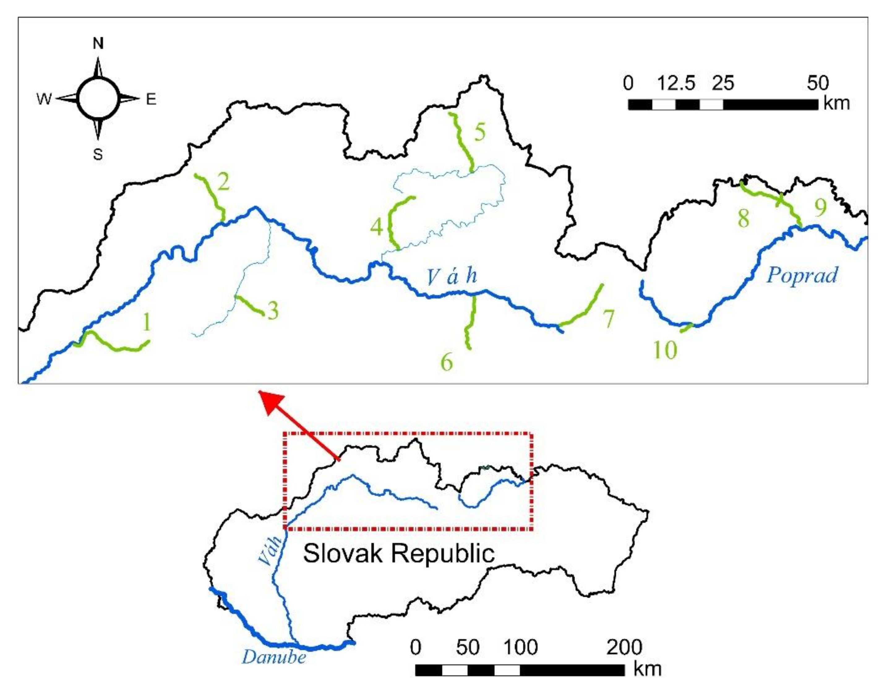
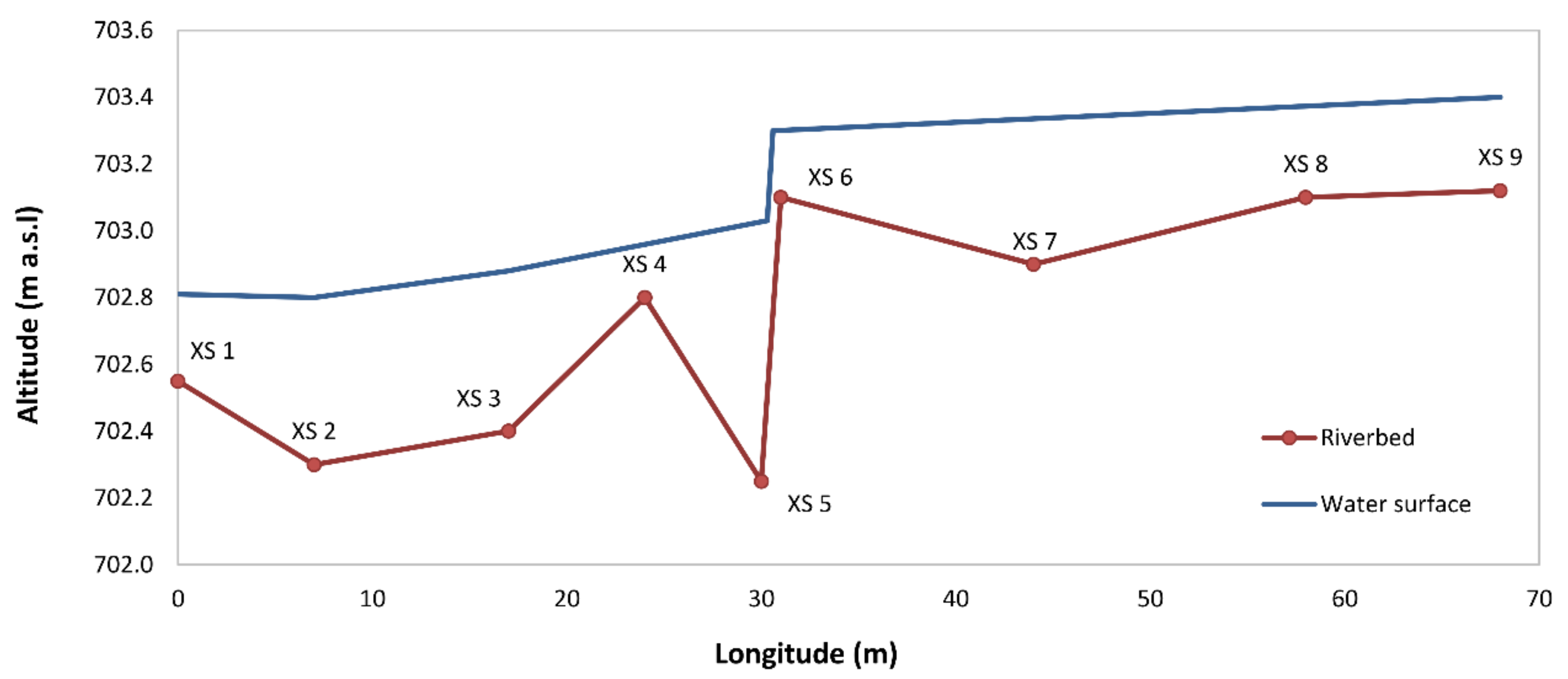
2.1. Reference Reaches of the Rivers

The reference reaches are located in the flysch area. For this study, smaller mountain and piedmont streams were selected for the following reasons:

• The effect of morphological changes has a negative effect on the biota of the stream, especially during minimum flow periods [26].
• Mountain streams are located in the upper sections of the river basin. Their length is relatively short, so the pollution load is low, and the water quality is usually suitable for the full use of the restoring effect on the stream and its surroundings [27].
• River regulation mainly affects the morphology of a stream. The good water quality of the selected reaches of mountain and piedmont streams does not alter the impact of the morphology on the quality of the aquatic habitat [28].

Influence of riverbed morphology on the quality of aquatic habitat, as well as analysis of quality evaluation according to various methods, was carried out on the following streams: Teplička (1), Lesnianka (2), Petrovička (3), Zázrivka (4), Veselianka (5), Kľačianka (6), Hybica (7), Lipnik (8), Kamienka (9), and Teplica (10). The location of selected streams is shown in Figure 1. The results of the ichthyological survey are stated in [15].

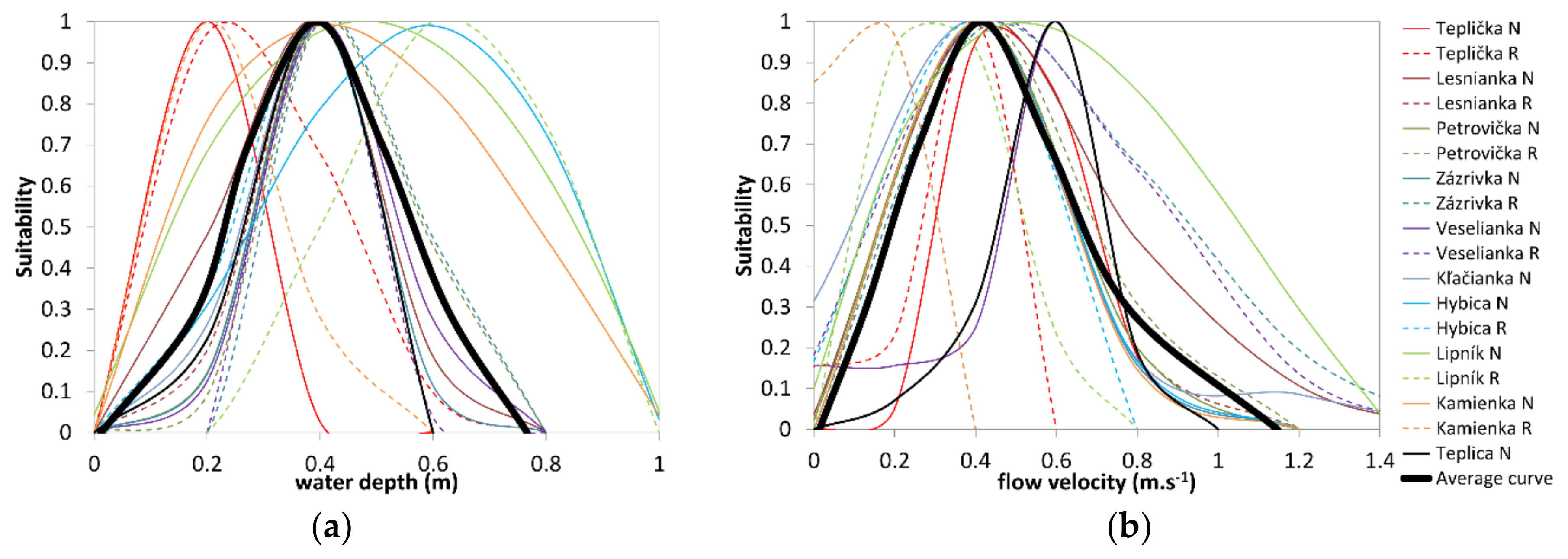
2.2. Influence of the Stream Characteristics on the Quality of the Aquatic Habitat

Based on the technical interventions in the stream, the quality of the aquatic habitat was assessed using the IFIM [11] by a RHABSIM model [25].

Habitat preference by fish is represented by the habitat suitability curves. They have been generalized for the adult BT. Peaks of the suitability curves, which represent the places with the highest occurrence of a given species at a certain depth and velocity, were compared. In the following, these values are referred to as the velocity parameter—P_v and the depth parameter—P_d. P_v and P_d values were derived from the set of suitability curves shown in Figure 2 for mountain streams in Slovakia. The result of the RHABSIM simulation was the evaluation of the habitat quality represented by the weighted usable area (WUA). It expresses a change in habitat quality relative to a variable parameter, usually a flow rate or a change in a channel’s morphology. The WUA image along the flow length had a mosaic shape composed of cells. WUA expresses the functional relationship between the flow and the unit area of the microhabitat for BT. The partially weighted usable area was then determined separately by multiplication of the cell surface (S_b) and the combined suitability factor (CSF):

$$\mathrm{WUA}=S_b\times CSF$$

(1)

There are several ways to determine the CSF. The simplest one is to multiply the depth and velocity parameters, which directly represent the quality of the habitat, after multiplying by the surface area:

$$CSF=\left(P_v\times P_d\times P_a\right)$$

(2)

where P_v is a velocity parameter, P_d is a depth parameter, and P_a is a parameter for habitat supplementary attributes (shelter and bottom substrate). Values of parameters P_v and P_d are determined from the velocity and depth suitability curves, and they range from 0 to 1. The method for calculating the CSF using a geometric average is expressed by the equation:

$$CSF={(P_v\times P_d\times P_a)}^{0.333}$$

(3)

Equation (3), same as Equation (2), assumes the equal weight of the individual parameters. This does not correspond to the reality, because individual parameters have different influences on the quality of the aquatic habitat. Next method based on determining the weighted average is defined as:

$$CSF=\frac{\left(P_v\times V_v\right)+\left(P_d\times V_d\right)+\left(P_a\times V_a\right)}{\left(V_v+V_d+V_a\right)}$$

(4)

where V_v is the weight for the velocity parameter, V_d is the weight for the depth parameter, and V_a is the weight for the attribute parameter (we can assign a certain weight to each parameter from 0.1 to 1). The advantage of Equation (4) is the possibility to define the weight of individual parameters.

3. Results

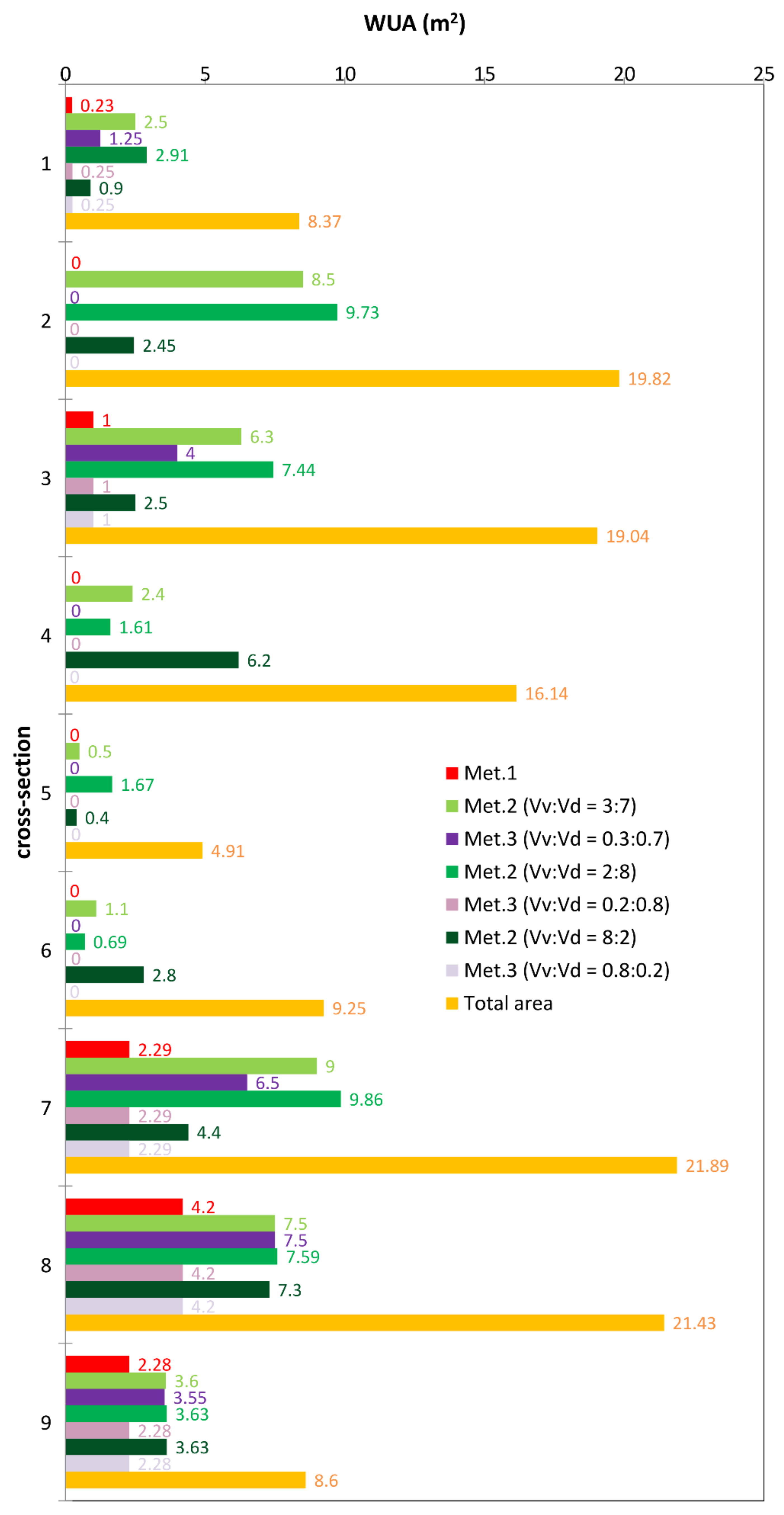
3.1. Evaluation of WUA

The WUA had been evaluated for all 18 reference reaches given in Figure 2, separately for flow velocity and water depth and as a combined suitability. Additionally, the total weighted usable area was determined. As an example, the degree of suitability for water depth, flow velocity, and the combined suitability for the BT in the Teplica River are shown in Figure 3.

The analysis of the results suggests that, when the degree of suitability for water depth is high, the combined suitability is almost zero due to a low flow velocity suitability. Figure 3 shows an example (suitability for the selected cell is marked in red color): When the depth suitability P_d (Figure 3a) takes the value 0.8 and the velocity suitability P_v (Figure 3b) takes the value 0.0, then the combined suitability (Figure 3c) takes the value 0.0.

Based on the above flaw, the change in the WUA was examined as the change of the weight of the velocity and depth parameters. The effect of the change of the parameter weight was analyzed by modifying the basic relationship (first method), which has the following form:

$$CSF=\left(P_v{}^{V_v}\times P_d{}^{V_h}\times P_a{}^{V_a}\right)$$

(5)

on the condition that

$$V_v+V_d+V_a=1$$

(6)

For simplicity, the calculation of the CSF according to Equation (2) is referred to as Method 1, the calculation of the CSF as a weighted average (Equation (4)) as Method 2, and the calculation of the CSF according to the modified Equation (5) as Method 3.

3.2. Determination of the Weight of the Parameters of Velocity and Depth

The analysis of the calculation of the WUA in the previous chapter shows that Method 1 (equivalence of individual factors) does not objectively evaluate the real quality of a habitat. This is also seen in Figure 3, where we get a generally unsuitable habitat by combining habitats that are suitable according to the depth and velocity parameters (Figure 3c). BT prefers shelters with sufficient depths. During low-flow periods, flow velocity is not decisive in areas with greater depths, as there are generally areas with low velocities (hiding places). Deep pools have a large flow area; therefore, the local flow velocities are usually close to 0 (a frequent case in pools). Despite this fact, this does not affect the preference of BT. In addition, it can be stated that the water depth at low flow rates has a significantly higher impact on habitat quality than velocity. Determining the weight of these parameters is an essential step to objectifying the weighted usable area according to the weighted average method. The effect of flow velocity and water depth on habitat availability has been verified for more flows. In the following section, the influence of the weight of the parameters of velocity and depth on the quality of the aquatic habitat is documented on the Teplica River.

The reference reach of the Teplica River was located below the village of Spišská Teplica. The Teplica River has a natural character with a ragged bottom morphology, which creates an alternating of riffle areas with slower areas. In the Teplica River, these areas are characterized by cross-sections 1, 4, and 6 (Figure 4). The areas with greater water depths and lower velocities are characterized by cross-sections 2, 3, 5, 7, 8, and 9 (Figure 4). Cross-sections 4 and 6 had low water depths and higher velocities. In these cross-sections, the WUA was lower.

Figure 5 shows a comparison of the WUA based on the various weights given by the three methods. The WUA calculated according to Method 1 is shown in red. In cross-sections 2, 4, 5, and 6, the WUA was zero; despite a good fit for depth, there was no suitability for velocity. The second method evaluated the habitat quality more objectively (Figure 5—light green color). Despite zero suitability for velocity, the WUA value was greater than zero. This represents the real result, since fish have been caught in these reaches; it means that this reach was accepted by the bioindicator, the fish. The third method (Figure 5—violet color) also appeared less suitable in this case. At zero velocity values, WUA was zero, similar to the first method. Therefore, Method 2 was used for further weight analyses and was compared to Method 1.

Based on previous analyses and results, it can be assumed that the depth parameter will have a higher weight than the velocity parameter. Figure 5 shows a comparison of the different parameter weights in determining the WUA using Method 1 and Method 2. The significant difference in the WUA is particularly noticeable in cross-section 2, where the WUA according to Method 1 was zero (due to zero velocity parameter values), while, according to Method 2, the WUA reached almost the highest values for the monitored reach. The opposite situation could be seen in cross-sections 4 and 6. In these cross-sections, the water depth was smaller, and the flow velocity was higher; such reaches do not create a suitable habitat during low flow rates. A different case may also occur, for example, in cross-sections 4 and 6 (Figure 5) when the WUA is greater at a ratio of V_v:V_d = 3:7 than at a ratio of V_v:V_d = 2:8. In these cross-sections, the water depths for the observed species were less acceptable, and the velocities were very favorable. When evaluating the total WUA for a selected reach of the Teplica River, it follows then that the higher the weight for the depth parameter, the greater the WUA (Figure 5).

Table 1. Comparison of the flow velocity and water depth parameters of the Teplica River at the flow rate that was measured during the field survey. XS—cross-sections from Figure 4, Point No.—points in cross-sections (only points where the value of the water depth or flow velocity parameters were greater than 0.4 are selected), Stationing—upstream stationing of the XS, Altitude—altitude of the riverbed bottom at a given point, v—flow velocity in point, P_v—velocity parameter, d—water depth in point, P_d—depth parameter, S_b—cell surface from Equation (1), weighted usable area (WUA) Method 1—WUA according to Equation (2), WUA Method 2—WUA according to Equation (4), and Total XS Area—total cross-section area.

XS	Point No.	Stationing (m)	Altitude (m a.sl.)	v (m·s−1)	Pv	d (m)	Pd	Sb (m2)	WUA Method 1 (m2)	WUA Method 2 (m2)	Total XS Area (m2)
1	3	2.9	702.5	0.24	0.1	0.29	0.7 1	3.15	0.23	1.86
	4	3.8	702.5	0.22	0.0	0.24	0.4 1	3.08	0.00	1.04
	XS Total								0.23	2.91	8.37
2	3	3.9	702.4	0.17	0.0	0.46	0.9 1	4.08	0.00	2.94
	4	4.4	702.3	0.17	0.0	0.45	0.9 1	5.76	0.00	4.30
	5	5.1	702.4	0.13	0.0	0.35	0.9 1	2.56	0.00	1.91
	XS Total								0.00	9.73	19.82
3	3	3	702.7	0.22	0.0	0.32	0.8 1	5.61	0.02	3.65
	4	3.6	702.4	0.27	0.2	0.42	1.0 1	4.42	0.98	3.66
	XS Total								1.00	7.44	19.04
4	4	2.4	702.8	0.46	0.9 1	0.18	0.0	4.06	0.00	0.72
	5	3	702.8	0.45	0.9 1	0.17	0.0	4.55	0.00	0.78
	XS Total								0.00	1.61	16.14
5	3	1.5	702.7	0.18	0.0	0.51	0.7 1	1.43	0.00	0.80
	5	2.3	702.3	0.11	0.0	0.39	1.0 1	1.09	0.00	0.85
	XS Total								0.00	1.67	4.91
6	3	1.4	703.2	0.74	0.6 1	0.08	0.0	2.73	0.00	0.34
	5	2.4	703.1	0.64	0.9 1	0.09	0.0	1.50	0.00	0.27
	XS Total								0.00	0.69	9.25
7	3	0.8	702.9	0.28	0.2	0.45	0.9 1	5.87	1.29	4.65
	4	1.3	702.9	0.27	0.2	0.38	1.0 1	5.13	1.00	4.21
	XS Total								2.29	9.86	21.89
8	3	1.1	703.1	0.33	0.4 1	0.27	0.6 1	5.88	1.48	3.19
	4	1.6	703.1	0.37	0.6 1	0.28	0.6 1	7.08	2.72	4.41
	XS Total								4.20	7.59	21.43
9	3	1.3	703.1	0.38	0.6 1	0.30	0.8 1	3.46	1.69	2.55
	4	1.9	703.1	0.36	0.6 1	0.24	0.4 1	2.42	0.59	1.08
	XS Total								2.28	3.63	8.60

¹ The cross-sections where the suitability for depth or velocity exceeded 0.4.

shows the output of the RHABSIM model to which the WUA values have been supplemented according to different methods. For the second method, the weight ratio for the parameters V_v:V_d was 2:8. The cross-sections, where the suitability for depth or velocity exceeded 0.4, are indicated by Table 1. The values of the velocity parameters in cross-sections 4 and 6 indicate more suitable velocities and unsuitable water depths. The comparison of Table 1 with Figure 6 clearly shows the areas of microhabitats with a suitability greater than 0.4 (>0.4 = green, >0.6 = yellow, >0.8 = orange, and 1 = red). For example, in cross-section 2, three areas with a suitability of 0.9 are shown in orange (Figure 6b).

4. Discussion

The analysis of the effect of abiotic parameters was aimed at determining the specific parameter weights when assessing the effect of flow on suitability curves.

Research of the water depth preferences of individual fish species has been conducted by several authors [11]. The occurrences of adult brown trout are bound to greater water depths (>30 cm), which were also confirmed by previous results [24]. Additionally, the velocity of water is not critical. Based on these findings, we can assign different weights to these abiotic parameters in any IFIM model so that the most important abiotic parameter of a habitat is reasonably considered.

From the results of the study [15], it follows that there is a strong dependence between habitat and water depth and a low dependence on flow velocity. Based on the above results, a change in habitat quality, according to three methods, was examined. Methods 1 and 3 had a common drawback; if one parameter was inappropriate—for example, the parameter equals 0—the entire CSF value became zero. The results in Table 1 also confirm this fact. However, this is contrary to reality. A natural stream has a ragged channel bed morphology that is important for a diverse fish population [29]. Different weights of parameters for water depth and flow velocity have been compared. If the quality of the habitat is assessed based on the depth parameter only, it could happen that the flow velocity would be so low that the riverbed begins to clog with fine-grained material, which is not suitable for BT. It means that the velocity parameter also affects the quality of the habitat. At low flow rates, there are many shells and shelters where the velocity is low, or almost zero, but the ichthyofauna prefer these areas. Therefore, it is necessary to choose the method that optimally characterizes the influence of individual parameters. It is necessary to avoid methods where one inappropriate parameter eliminates the influence of other parameters. The abundance of adult BT was 1488 pieces per hectare in the reference reach of the Teplica River; other ichthyological data are given in [15]. This can be considered a good abundance according to Method 2. The optimal parameter ratio was investigated at 10 flow rates. The analysis shows that the optimum velocity-to-depth parameter ratio is 2:8.

The suitability of a habitat for a particular fish should be determined by combining hydrodynamic models with the characteristics of fish habitats [30].

The evaluation of the suitability of habitats for a particular fish, or its stage of life, was the subject of studies [31] or [32], which dealt with the modeling of habitat quality for ichthyofauna.

In this study, BT was chosen for the bioindication, because it was present in all 18 reference reaches in sufficient quantity, allowing the generalization of the suitability curves (Figure 2). The next most numerous species, Alpine Bullhead (Cottus poecilopus), was present in 16 reference reaches, but this species’ habitat preference of flow velocity or water depth is questionable. Altogether, 16 fish species were present in 18 reference stream reaches. More information on species diversity can be found in [15]. However, this was only a secondary argument for choosing the right fish species. The results of the preliminary research carried out in 52 reaches of 43 mountain and piedmont streams in the flysch area in Northern Slovakia, where the stream reaches described in this study are located, were decisive for the BT’s choice. From these results, it followed that the dominant variable for the brown trout in piedmont streams during low-flow periods was the water depth. Additionally, based on the results of other studies [33,34,35,36], it follows that an environmental flow assessment should not be based only on a hydrological assessment, but it should also include hydrogeomorphic processes that are directly related to aquatic ecosystem needs.

Stream restoration aimed at increasing riverbed raggedness contributes to increasing the species diversity, reduces the number of opportunistic species, and results in an overall increase in the health of fish [30].

There are many rainfall-runoff models by which it is possible to predict the flow rate development prognosis. However, there are few possibilities to assess the impact of the flow rate changes due to climate changes on the stream ecosystem. This research contributes to the objectivization of modeling and forecasting the impact of climate changes on the quality of aquatic habitats. An example of the prognosis of changes in aquatic habitat quality due to climate changes by the RHABSIM model can be found in [13].

5. Conclusions

This research contributes to the objectification of the evaluation of the quality of habitats in mountain and piedmont streams using the IFIM. The key step that has been generally neglected is to correctly illustrate the relationship between abiotic microhabitat variables, for what the several methods were tested using various mathematical expressions and different ratios.

It is realistic to assume that, when using a weighted average method with a velocity-to-depth parameter ratio equal to 2:8, we can obtain results that are close to reality—or will, at the least, be substantially more objective than using other methods (Methods 1 and 3), which are implicitly defined in the RHABSIM model. Further research can be focused on the possibilities of transferability to other similar groups of streams, potentially using other fish species.

References

1. Rosenfeld, J.S.; Ptolemy, R. Modelling available habitat versus available energy flux: Do PHABSIM applications that neglect prey abundance underestimate optimal flows for juvenile salmonids? Can. J. Fish. Aquat. Sci. 2012, 69, 1920–1934. [Google Scholar] [CrossRef]
2. Brachet, C.; Magnier, J.; Valensuela, D.; Petit, K.; Fribourg-Blanc, B.; Bernex, N.; Scoullos, M.; Tarlock, D. The Handbook for Management and Restoration of Aquatic Ecosystems; International Network of Basin Organizations: Paris, France; Global Water Partnership: Stockholm, Sweden, 2015. [Google Scholar]
3. Farnsworth, J.M.; Baasch, D.M.; Farrell, P.D.; Smith, C.B.; Werbylo, K.L. Investigating whooping crane habitat in relation to hydrology, channel morphology and a water-centric management strategy on the central Platte River, Nebraska. Heliyon 2018, 4, e00851. [Google Scholar] [CrossRef]
4. Galie, A.-C.; Moldoveanu, M.; Antonalu, O. Hydromorphological Assessment of Atypical Lowland River—Romanian Litoral Basin Case Study. Carpathian J. Earth Environ. Sci. 2017, 12, 161–169. [Google Scholar]
5. Carnie, R.; Tonina, D.; McKean, J.A.; Isaak, D. Habitat Connectivity as a Metric for Aquatic Microhabitat Quality: Application to Chinook Salmon Spawning Habitat. Ecohydrology 2016, 9, 982–994. [Google Scholar] [CrossRef]
6. Gibson, S.A.; Pasternack, G.B. Selecting Between One-Dimensional and Two-Dimensional Hydrodynamic Models for Ecohydraulic Analysis. River Res. Appl. 2016, 32, 1365–1381. [Google Scholar] [CrossRef] [Green Version]
7. Belčáková, I. Strategic Environmental Assessment—An instrument for better decision-making towards urban sustainable planning. Procedia Eng. 2016, 161, 2058–2061. [Google Scholar] [CrossRef] [Green Version]
8. Belčáková, I.; Pšenáková, Z. Specifics and landscape conditions of dispersed settlements in Slovakia—A case of natural, historical and cultural heritage. In Best Practices in Heritage Conservation and Management. From the World to Pompeii: Le vie dei Mercanti: XII Forum Internazionale di Studi; Gambardella, C., Ed.; La Scuola di Pitagora Editrice: Napoli, Italy, 2014; pp. 261–268. ISBN 978-88-6542-347-9. [Google Scholar]
9. Ivan, P.; Macura, V.; Belčáková, I. Various approaches to evaluation of ecological stability. In Proceedings of the International Multidisciplinary Scientific GeoConference SGEM. Ecology and environmental protection, Albena, Bulgaria, 17–26 June 2014; Abstract Number 5/109. pp. 799–805. [Google Scholar]
10. Jakubcová, A.; Grežo, H.; Hrešková, A.; Petrovič, F. Impacts of Flooding on the Quality of Life in Rural Regions of Southern Slovakia. Appl. Res. Qual. Life 2016, 11, 221–237. [Google Scholar] [CrossRef]
11. Bovee, K.D.; Lamb, B.L.; Bartholow, J.M.; Stalnaker, C.B.; Taylor, J. Stream Habitat Analysis Using the Instream Flow Incremental Methodology; Information and Technology Report No. USGS/BRD-1998-0004; U.S. Geological Survey: Denver, CO, USA, 1998; p. 131. [Google Scholar]
12. Ayllón, D.; Railsback, S.F.; Vincenzi, S.; Groeneveld, J.; Almodóvar, A.; Grimm, V. InSTREAM-Gen: Modelling eco-evolutionary dynamics of trout populations under anthropogenic environmental change. Ecol. Model. 2016, 326, 36–53. [Google Scholar] [CrossRef]
13. Macura, V.; Štefunková, Z.; Škrinár, A. Determination of the effect of water depth and flow velocity on the quality of an in-stream habitat in terms of climate change. Adv. Meteorol. 2016. [Google Scholar] [CrossRef] [Green Version]
14. Keeley, E.R.; Campbell, S.O.; Kohler, A.E. Bioenergetic calculations evaluate changes to habitat quality for salmonid fishes in streams treated with salmon carcass analog. Can J. Fish. Aquat. Sci. 2016, 73, 819–831. [Google Scholar] [CrossRef]
15. Štefunková, Z.; Belčáková, I.; Majorošová, M.; Škrinár, A.; Vaseková, B.; Neruda, M.; Macura, V. The impact of the morphology of mountain watercourses on the habitat preferences indicated by ichtyofauna using the IFIM methodology. Appl. Ecol. Environ. Res. 2018, 16, 5893–5907. [Google Scholar] [CrossRef]
16. Kovacevic, A.; Latombe, G.; Chown, S.L. Rate dynamics of ectotherm responses to thermal stress. Proc. R. Soc. B 2019, 286, 20190174. [Google Scholar] [CrossRef] [PubMed] [Green Version]
17. Jarić, I.; Lennox, R.J.; Kalinkat, G.; Cvijanović, G.; Radinger, J. Susceptibility of European freshwater fish to climate change: Species profiling based on life-history and environmental characteristics. Glob. Chang. Biol. 2019, 25, 448–458. [Google Scholar] [CrossRef] [PubMed] [Green Version]
18. Conallin, J.; Boegh, E.; Jensen, J.K. Instream physical habitat modelling types: An analysis as stream hydromorphological modelling tools for EU water resource managers. Intl. J. River Basin Manag. 2010, 8, 93–107. [Google Scholar] [CrossRef] [Green Version]
19. Trull, N.; Böhm, M.; Carr, J. Patterns and biases of climate change threats in the IUCN Red List. Conserv. Biol. 2018, 32, 135–147. [Google Scholar] [CrossRef] [PubMed]
20. Maddock, I.; Harby, A.; Kemp, P.; Wood, P.J. Ecohydraulics: An Integrated Approach; John Wiley & Sons: Hoboken, NJ, USA, 2013. [Google Scholar] [CrossRef]
21. Hohensinner, S.; Hauer, C.; Muhar, S. River Morphology, Channelization, and Habitat Restoration. In Riverine Ecosystem Management; Aquatic Ecology, Series; Schmutz, S., Sendzimir, J., Eds.; Springer: Cham, Switzerland, 2018; Volume 8. [Google Scholar] [CrossRef] [Green Version]
22. Štefunková, Z.; Škrinár, A.; Belčáková, I.; Halaj, P.; Ivan, P. Determination of the Qualitative Features of Watercourses for Restoration in the Urban Environment. Procedia Eng. 2016, 161, 23–29. [Google Scholar] [CrossRef] [Green Version]
23. Thomas, J.A.; Bovee, K.D. Application and testing of a procedure to evaluate transferability of habitat suitability criteria. Regul. Rivers Res. Manag. 1993, 8, 285–294. [Google Scholar] [CrossRef]
24. Macura, V.; Škrinár, A.; Kaluz, K.; Jalčovíková, M.; Škrovinová, M. Influence of the morphological and hydraulic characteristics of mountain streams on fish habitat suitability curves. River Res. Appl. 2012, 28, 1161–1178. [Google Scholar] [CrossRef]
25. Payne, T.R. RHABSIM: User friendly computer model to calculate river hydraulics and aquatic habitat. In Proceedings of the First International Symposium on Habitat Hydraulics, Trondheim, Norway, 18–20 August 1994; The Norwegian Institute of Technology: Trondheim, Norway, 1994; pp. 254–260. [Google Scholar]
26. Schmutz, S.; Bakken, T.H.; Friedrich, T.; Greimel, F.; Harby, A.; Jungwirth, M.; Melcher, A.; Unfer, G.; Zeiringer, B. Response of Fish Communities to Hydrological and Morphological Alterations in Hydropeaking Rivers of Austria. River Res. Appl. 2015, 319, 919–930. [Google Scholar] [CrossRef] [Green Version]
27. Pandey, P.; Soupir, M.L.; Wang, Y.; Cao, W.; Biswas, S.; Vaddella, V.; Atwill, R.; Merwade, V.; Pasternack, G. Water and Sediment Microbial Quality of Mountain and Agricultural Streams. J. Environ. Qual. 2018, 47, 985–996. [Google Scholar] [CrossRef] [Green Version]
28. Ernst, A.G.; Baldigo, B.P.; Mulvihill, C.I.; Vian, M. Effects of Natural-Channel-Design Restoration on Habitat Quality in Catskill Mountain Streams, New York. Trans. Am. Fish. Soc. 2010, 139, 468–482. [Google Scholar] [CrossRef]
29. El-Jabi, N.; Caissie, D. Characterization of natural and environmental flows in New Brunswick, Canada. River Res. Appl. 2019, 35, 14–24. [Google Scholar] [CrossRef] [Green Version]
30. Favata, C.A.; Maia, A.; Pant, M.; Nepal, V.; Colombo, R.E. Fish assemblage change following the structural restoration of a degraded stream. River Res. Appl. 2018, 34, 927–936. [Google Scholar] [CrossRef] [Green Version]
31. Miranda, L.E.; Killgore, K.J.; Slack, W.T. Spatial organization of fish diversity in a species-rich basin. River Res. Appl. 2019, 35, 188–196. [Google Scholar] [CrossRef]
32. Zhang, P.; Cai, L.; Yang, Z.; Chen, X.; Qiao, Y.; Chang, J. Evaluation of fish habitat suitability using a coupled ecohydraulic model: Habitat model selection and prediction. River Res. Appl. 2018, 34, 937–947. [Google Scholar] [CrossRef]
33. Wohl, E.; Lane, S.N.; Wilcox, A.C. The science and practice of river restoration. Water Resour. Res. 2015, 51, 5974–5997. [Google Scholar] [CrossRef] [Green Version]
34. Yarnell, S.M.; Petts, G.E.; Schmidt, J.C.; Whipple, A.A.; Beller, E.E.; Dahm, C.N.; Goodwin, P.; Viers, J.H. Functional flows in modified riverscapes: Hydrographs, habitats and opportunities. BioScience 2015, 65, 963–972. [Google Scholar] [CrossRef] [Green Version]
35. Zhang, L.; Yuan, B.; Yin, X.; Zhao, Y. The Influence of Channel Morphological Changes on Environmental Flow Requirements in Urban Rivers. Water 2019, 11, 1800. [Google Scholar] [CrossRef] [Green Version]
36. Seeteram, N.A.; Hyera, P.T.; Kaaya, L.T.; Lalika, M.C.S.; Anderson, E.P. Conserving Rivers and Their Biodiversity in Tanzania. Water 2019, 11, 2612. [Google Scholar] [CrossRef] [Green Version]
Figure 1. Localization of the reference reaches of the mountain streams in Slovakia.
Water 12 01131 g001
Figure 2. Suitability curves for (a) water depth and (b) flow velocity on the mountain streams of Slovakia. Natural streams (N) are represented by solid lines, and regulated streams (R) are indicated by dashed lines. The average suitability curve is shown by a thick, black line—adapted from [15].
Water 12 01131 g002
Figure 3. Suitability of the brown trout (BT) in the Teplica River for (a) water depth, (b) flow velocity, and (c) as a combined suitability. The red squares mark the suitability for selected cells and show how the combined weighted usable area (WUA) is calculated. The XS station is the upstream distance of the cross-sections.
Water 12 01131 g003
Figure 4. Longitudinal profile of the Teplica River. XS is the abbreviation for cross-section.
Water 12 01131 g004
Figure 5. Comparison of the WUA by three methods in individual cross-sections of the Teplica River (values in the histogram are given for Methods 1, 2, and 3; the total area is shown for comparison). Met.: method.
Water 12 01131 g005
Figure 6. Comparison of the suitability for (a) water depth and (b) flow velocity for BT at the measured flow rate of Q = 0.12 m3·s−1 in the Teplica River.
Water 12 01131 g006