Source Water Apportionment of a River Network: Comparing Field Isotopes to Hydrodynamically Modeled Tracers
by

Lily A. Tomkovic
1,*, 
Edward S. Gross
1,
Bobby Nakamoto
2,
Marilyn L. Fogel
2 and
Carson Jeffres
1 1
Center for Watershed Sciences, University of California Davis, 1 Shields Ave, Davis, CA 95616, USA
2
EDGE Institute, University of California Riverside; 900 University Ave, Riverside, CA 92521, USA
*
Author to whom correspondence should be addressed.
Water 2020, 12(4), 1128; https://doi.org/10.3390/w12041128
Submission received: 7 March 2020
/
Revised: 10 April 2020
/
Accepted: 13 April 2020
/
Published: 15 April 2020
(This article belongs to the Special Issue Tracer and Timescale Methods for Passive and Reactive Transport in Fluid Flows)
Abstract
:Tributary source water provenance is a primary control on water quality and ecological characteristics in branching tidal river systems. Source water provenance can be estimated both from field observations of chemical characteristics of water and from numerical modeling approaches. This paper highlights the strengths and shortcomings of two methods. One method uses stable isotope compositions of oxygen and hydrogen from water in field-collected samples to build a mixing model. The second method uses a calibrated hydrodynamic model with numerical tracers released from upstream reaches to estimate source-water fraction throughout the model domain. Both methods were applied to our study area in the eastern Sacramento–San Joaquin Delta, a freshwater tidal system which is dominated by fluvial processes during the flood season. In this paper, we show that both methods produce similar source water fraction values, implying the usefulness of both despite their shortcomings, and fortifying the use of hydrodynamic tracers to model transport in a natural system.
1. Introduction
Across the globe, people have settled and established communities beside estuaries and river deltas that have proven to be ideal habitats for humans, flora, and fauna [1]. Estuaries are unique habitats in a myriad of ways—they are the location where tidal influence extends into the riverine landscape, where saline seawater and fresh river water mix, and where geomorphic effects from marine processes meet fluvial erosion and deposition. All of these factors produce an ecosystem that is specially adapted to growth and success in this confluence of conditions. Even though estuaries support a large diversity of species, they are threatened habitats [2,3]. Numerous anthropogenic effects have impacted the quality of estuarine habitat [4]. For example, pollutants and anthropogenic inputs in the form of chemicals, human and agricultural wastes, and sediment have been introduced into the watersheds along their reaches [5,6]. Projected sea level rise [7] and massive diversions from natural riverine inputs [8] have impacted salinity dynamics, affecting ecosystem health [9]. Entire landscapes have been shifted from land to sea [10,11], affecting numerous processes from the headwaters of tributaries down to their deltas, all impacting the health of the estuary.
To combat these problems, humans have sought ways to balance their needs for the natural resources provided by estuaries with the long-term survival and fitness of those habitats. Better practices have been established to control pollution into rivers, estuaries, and marine environments. Furthermore, restoration efforts have been made in order to address the degradation of physical habitat surrounding river deltas and estuaries. Combinations of these efforts have been undertaken in order to produce multi-pronged benefits within these habitats. Often, the goal of restoration and management actions are to allow for the physical and biological processes important in estuaries to resume functioning. For instance, the restoration of off-channel habitat in the tributaries leading into an estuary provides the physical parameters (such as turbidity, dissolved oxygen, temperature, and light availability) to generate primary and secondary producers (phyto- and zoo-plankton) [12]. With proper connectivity, that productivity can flow into riverine habitat and be transported downstream throughout the estuary. Following the overall impacts of estuarine restoration is complicated, however, because of the complex physical properties of deltas and estuaries, such as reconnecting or braided river networks, tidal pumping effects [13], and salinity gradients.
Understanding where water flows and where it originates is useful for understanding what impacts a restoration project has as well as what the character of water is coming into a potential restoration site. Identifying source water fraction (SWF) of a river network addresses the spatiotemporal distribution of source waters and allows the investigation of tributary water fate. The properties of tributaries, such as the stable isotope compositions of water, have been used to identify source water distribution, but these studies have typically been applied to lakes or groundwater [14,15,16,17]. Other studies have used isotope signatures to identify which tributaries have dominant effects on geochemical properties of the mainstem [18], to investigate snowmelt versus rainfall contribution [19], and to identify water origin [20]. Our study aimed to use two methods to find the SWF at each location within the study area over time; one method used is similar to that of Halder et al. [21] and Marchina et al. [20], which evaluates stable hydrogen (2 and oxygen (18 isotopes at sample locations and compares those to the tributary source waters of interest.. Another direct application of using physical properties of tributary water to find the distribution of source waters in a river network was presented by Peter et al. [22] in a physically modeled hypothetical watershed. In the study, high-resolution mass spectrometry of organic contaminants was used to confirm the source hydrology of a hypothetical river system with known flows, and thus known mixtures. This physical model study demonstrated the potential of using physical and chemical signatures in water to identify source water, but was limited to systems with an exact knowledge of tributary discharge and mixing patterns, limiting the study to a discussion of methodology instead of an application of a real-world scenario in a river network. We address this limitation using a separate method to investigate the hydraulics and transport processes of a system in order to provide estimated flows and mixing patterns.
Hydrodynamic models are numerical tools that solve equations of motion in fluid mechanics and are widely used to replicate flood events and complex physical processes in river networks. Sridharan et al. [23] used a one-dimensional streamline-following junction model to evaluate particle paths through the Sacramento–San Joaquin Delta of California (Delta), giving insight to source-water fate at a large and broad scale. Bai et al. [24] used a three-dimensional hydrodynamic and water quality model to source-apportion different tributary contributions to nitrogen and phosphorous loads. The source-apportionment indicates the chemical impact of tributaries, but not their relative volume at any particular location. In order to test the validity of a field-based approach to identifying SWF in a river network, we developed a hydrodynamic model coupled with a transport model. This study’s comparison of methods can help address limitations of stable isotope methods of finding the SWF of a particular site, as well as demonstrating a field validation of source water tracking using hydrodynamic models.
This study centered on the McCormack-Williamson Tract (MWT), an island protected by a ring levee in the Delta, and the surrounding area. Slated for restoration, the site lies downstream of several other floodplain restoration sites along the Cosumnes River and Dry Creek, making understanding the distribution of incoming source waters helpful to improve the overall efficacy of the MWT restoration. Specifically, water that has had access to floodplains would likely carry more allochtonous material, providing more carbon and nutrients to kickstart in situ production at the study site. In this paper, we characterize the spatiotemporal distribution of SWF at different sites in and around the island while it was flooded. In the absence of measurements of individual tributary flows into the study area, indirect methods must be applied to estimate source water distribution. Our study aimed to evaluate the utility of the two methods discussed, to compare hydrodynamically derived values to in situ data, and to discuss the implication of these approaches to the Delta, as well as other riverine systems.
2. Methods
2.1. Study Area
The Sacramento–San Joaquin Delta (Delta), located in California, USA is a large, reconnecting, freshwater–tidal river network that leads into the San Francisco Bay Estuary. The Delta is a major economic asset to the state of California. Its major diversions of freshwater, mainly from the Sacramento River, provide irrigation for the state’s thriving agricultural industry, as well as drinking water for its cities [25]. These large diversions from the Delta, supported by an extensive system of reservoirs, have altered transport and seasonal salt intrusion trends in the estuary [26,27]. The nutrient-rich soils in the off-channel habitat of the Delta have been predominantly converted to agricultural plots [10], while at the same time over 95% of floodplain and intertidal habitat [28] have been channelized, thereby eliminating shallow-water habitat from the ecosystem. These and many other anthropogenic impacts on the Delta have motivated restoration efforts to mitigate the altered ecosystem. The restoration of shallow-water habitat can boost productivity, and understanding the transport of these enriched source waters is an important factor in maximizing restoration efforts [29], making Delta an ideal location for this study.
The specific area studied in this paper is in the North-East Delta near the confluence of the Mokelumne and Cosumnes Rivers (see Figure 1). It is a freshwater tidal system dominated by fluvial processes during the flood season by the upstream Dry Creek, Cosumnes, and Mokelumne watersheds. A major feature of the study site just west of the confluence is the McCormack-Williamson Tract (MWT), which was historically wetland habitat [30] but is now a 1400-acre ring-leveed property used for agricultural purposes. The MWT is slated for restoration to tidal and floodplain habitat. During the period of this study, an accidental breach occurred near the planned breach, allowing for flood flows through MWT along with intertidal habitat in non-flooding periods.
Just west of the MWT are the Delta Cross Channel Gates, which are a major feature of the Delta, controlling diversion of freshwater flows from the Sacramento River to the Southern Delta’s major pumping plants for municipal, agricultural, and other export across California. North of the MWT are Middle, Lost, and Snodgrass Sloughs. Snodgrass Slough is the drainage for Morrison Creek and the Stone Lake National Wildlife Refuge, where the stream enters the Delta. Middle and Lost Sloughs are dead-end sloughs during non-flooding periods and convey Cosumnes overland flow during floods. The Cosumnes River is the only major river coming out of the Sierra Nevada Range without a major dam, allowing for a relatively natural hydrograph with natural overbank/floodplain flow [31]. Due to this hydrograph and a variety of restoration actions, the Cosumnes River provides floodplain rearing for a variety of native juvenile fishes and exports productivity downstream [32]. This relatively natural system dramatically differs from the other major stream source to the study area—the Mokelumne River. The Mokelumne River is a 5550 km2 watershed and has its headwaters in the Sierra Nevada Range extending down to the San Joaquin River in the Delta. River flow in the lower 55 km is regulated by Camanche Reservoir and conveyed to the confluence of the San Joaquin River through a leveed channel.
For this study, we developed two types of modeling methods to investigate the SWF of Mokelumne River water and Cosumnes River Water (locations shown in Figure 2).
2.2. SWF Method I: Isotope Mixing Model
2.2.1. Mixing Model Theory
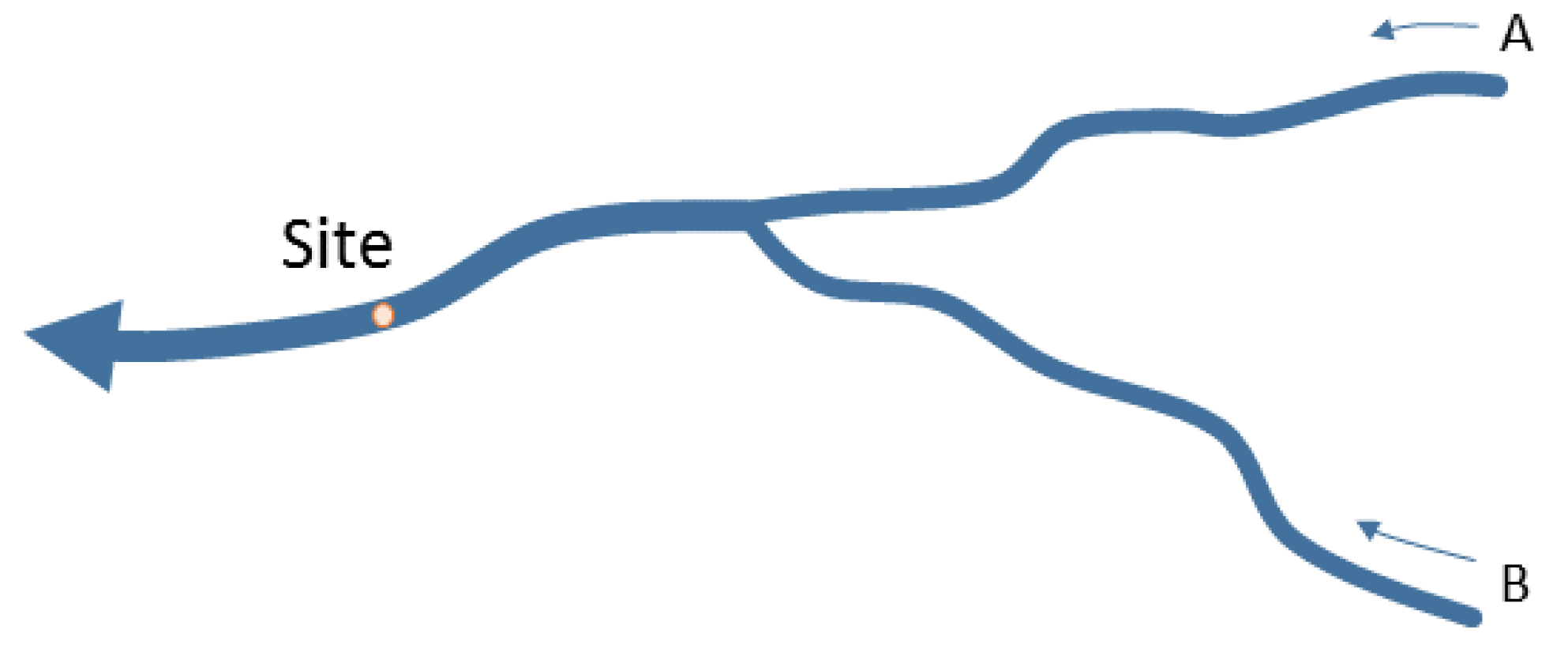
Following Gibson et al. [14], a mass balance approach was used to estimate the volumetric fraction of two tributary waters at downstream sample site (Figure 3). The mixing model asserts that the isotopic composition at the sample site is a volume-weighted average of tributary isotopic composition.
where , , and are the volumetric fraction of River “A”, River “B”, and whichever site was being analyzed, respectively. The isotopic composition, in delta notation, of each location is denoted as , where is either or . After assuming that , the SWF for River “A” or “B” at any given site is:
This mixing model applies to samples with or . In the event that this condition was not met the sample was not included in the analysis. In addition, the mixing model assumes that the isotopic composition of rivers A and B are stationary, that local effects on (e.g., isotopic fractionation via evaporation) are negligible [33], and that the sampled water is comprised entirely of contributions from the two tributaries.
2.2.2. Field Data—Collecting Isotope Samples
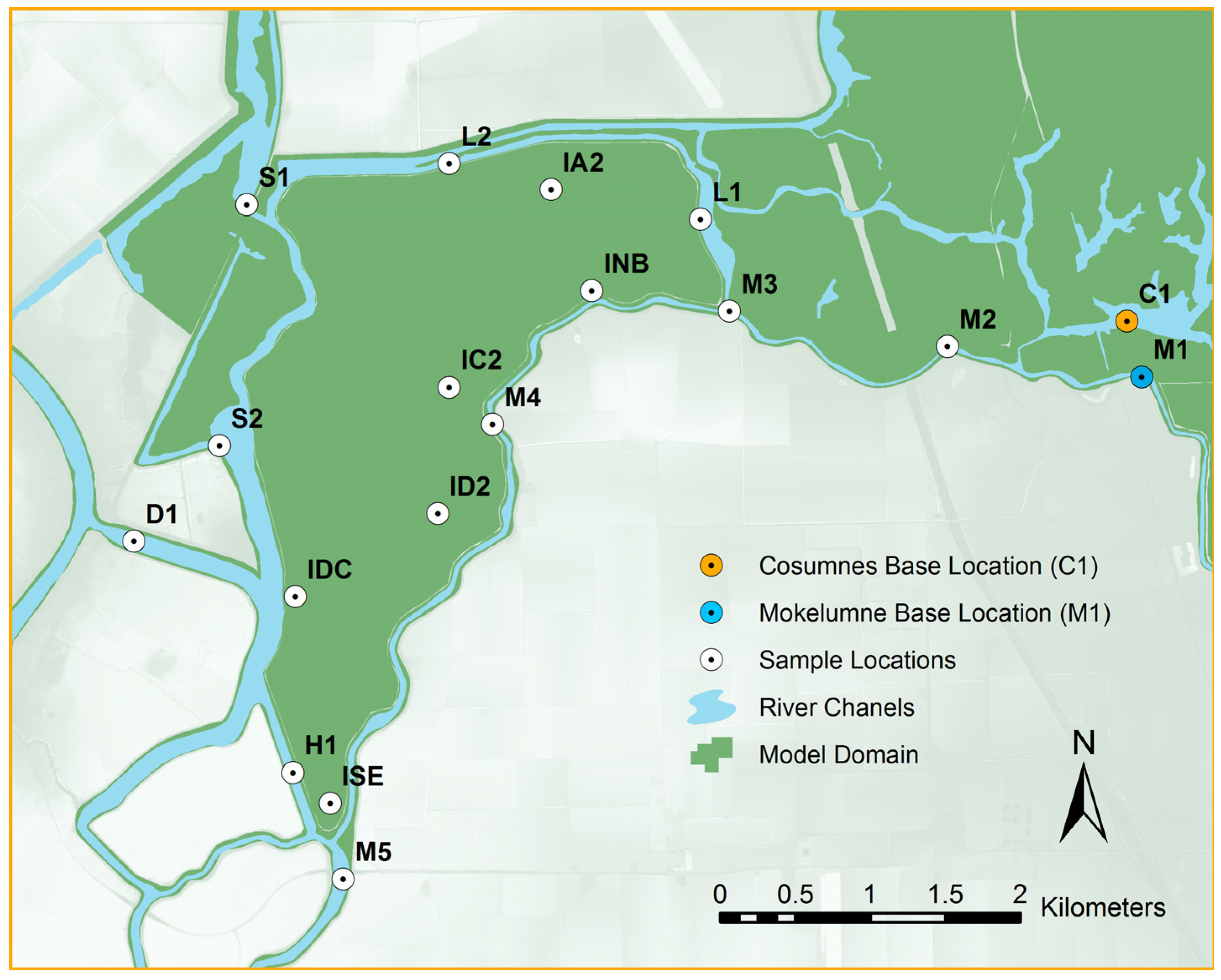
The field campaign at the MWT sampled the water biweekly from August 2016 to June 2019 at 18 locations (Figure 2). Not all locations were sampled throughout the entire period, due to a variety of reasons. The MWT locations (those that start with “I”) were only sampled during the MWT’s breach from February 2017 to June 2017. At each location, a grab sample of water was taken from the top ~0.25 m of water, filtered through glass fiber (GF/F) filters (nominal pore size: 0.7 microns) and stored refrigerated until isotopic analysis was performed.
2.2.3. Isotope Processing
We used delta notation ( and to characterize our samples. and values change with precipitation elevation, evaporation, and other hydrologic factors, often making them differ significantly between watersheds. Delta notation describes the relative composition of stable isotopes in the sample through the formula: δnX = __‰ = (Rsample/Rstandard − 1) × 1000; where n is the atomic number of the heavy isotope in question and Rsample and Rstandard represent the ratio of the heavy isotope (here, 2H and 18O) to the light isotope (here, 1H and 16O) in the sample and the international standard, respectively. We determined and via off-axis integrated cavity output spectroscopy (Los Gatos Research (LGR), Liquid Water Isotope Analyzer) at the University of California Merced. Working standards from LGR, calibrated against National Institute of Standards and Technology (U.S. Department of Commerce) reference materials (Vienna Standard Mean Ocean Water (VSMOW), Greenland Ice Sheet Precipitation (GISP), and Standard Light Antarctic Precipitation (SLAP)), were analyzed throughout and used to correct measured isotope ratios, so they could be expressed relative to the international standard: VSMOW. Four different standards ranging from = −9.2; = −2.7 to ( = −154.0; = −19.5 were used as internal standards. Raw data was processed using LWIA post-analysis software (LGR).
Each time we determined the isotopic ratio of a water sample or standard, it was analyzed via repeated injections. The standard deviation of our measured values (n = 89) for standards was 0.3 ± 0.1 and 0.06 ± 0.01 for δ2H and δ18O, respectively. Averaging multiple injections per sample was effective at reducing uncertainty originating from small injection-to-injection differences, indicating high precision. Furthermore, our mean measured values differed from known standard values by only 0.03 and 0.01 for δ2H and δ18O respectively; indicating high accuracy, even when the above uncertainties are considered. Propagation of uncertainty into our model is addressed in Section 4.
2.2.4. Application of Mixing Model
2.3. SWF Method II: Hydrodynamic Model
The second method of finding SWF in a natural system uses a two-dimensional hydrodynamic model coupled with a transport model that can transport a contaminant tracer with advection and diffusion. In this approach, the transport model releases conservative tracers in the tributaries of interest (Rivers “A” and “B” in Figure 3), which are tracked throughout the model domain in time. The summation of all tracer fractions at any given location is 1.0, allowing for a simple numerically based volumetric fraction of the tributary source waters.
2.3.1. Hydrodynamic Model Development
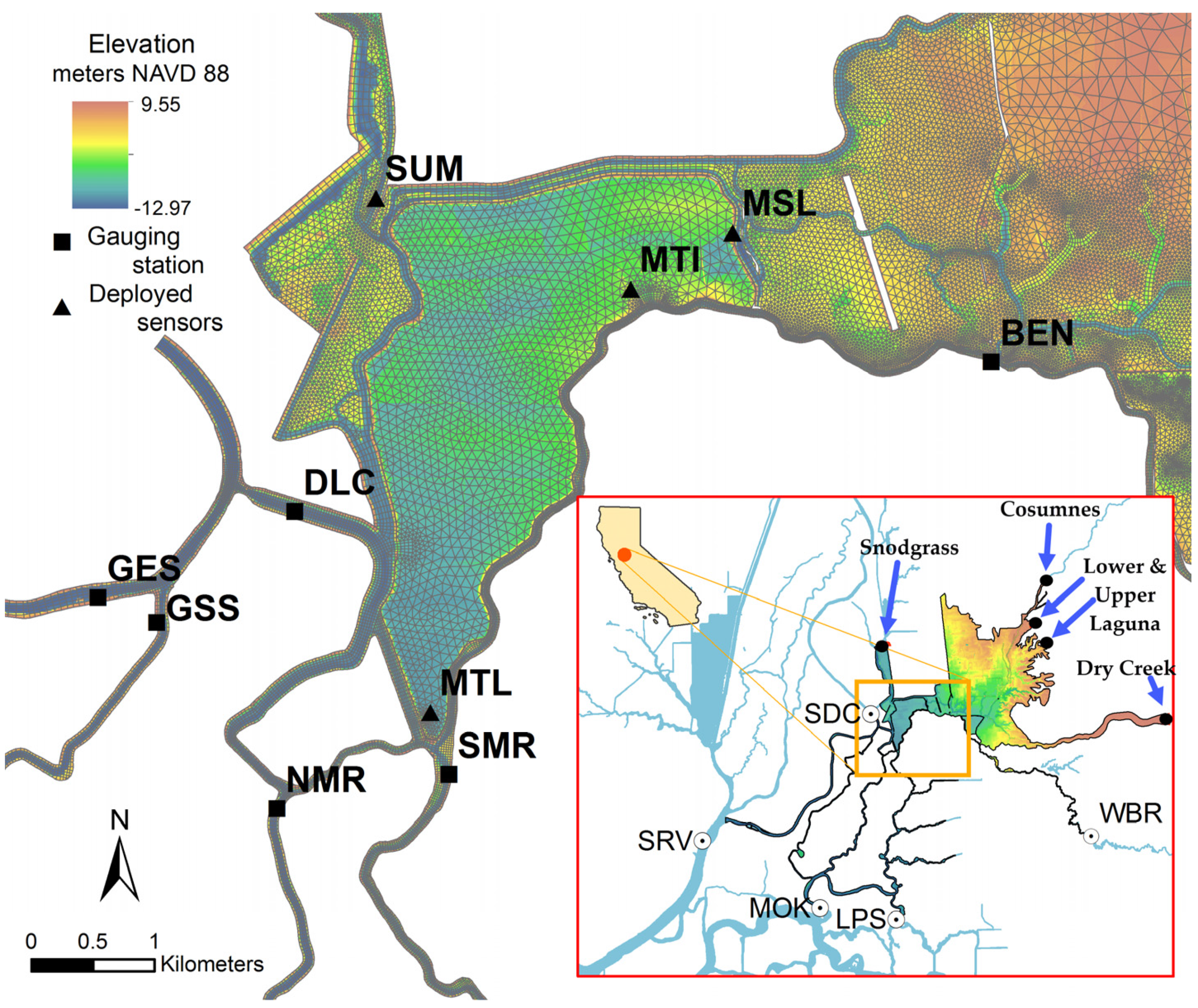
A two-dimensional hydrodynamic model was built and calibrated using UnTRIM [34]. The two-dimensional version of UnTRIM uses a semi-implicit algorithm for the depth-averaged shallow water equations under a hydrostatic assumption [35]. The mesh was generated using Preprocessor Janet (http://www.smileconsult.de) and contains quadrilateral and triangular elements, Figure 1) with a total of 109,129 elements. The average edge length was around 30 m with the smallest element being 3 m and the largest being over 200 m in an area insignificant to this study.
The three stage boundaries at the downstream end were set using observed gages. On the Sacramento River the boundary was set within 3 km of the United States Geological Survey (USGS) gage SRV-Sacramento River at Rio Vista-11455420 and the gage data was used directly. The other two downstream boundaries’ gages (USGS gages MOK-Mokelumne R A Andrus Island NR Terminous CA-11336930 and LPS-Little Potato Slough at Terminous-11336790) were located at the model boundary directly, but did not use a known datum, so the reported time series were adjusted using calibration offsets from a larger Delta-wide model.
2.3.2. Boundary Condition Development
The seven upstream flow boundaries used either gaged data or were calculated. The USGS discharge gages SDC-Sacramento R above Delta Cross Channel-11447890 and WBR-Mokelumne R A Woodbridge CA-11325500 were used at the upstream ends of the Sacramento and Mokelumne Rivers, respectively. The discharge boundary at Snodgrass Slough was calculated using lagged discharge data from USGS MFR-Morrison C NR Sacramento CA-1136580. The boundaries at the Cosumnes River, Upper Laguna Creek, Lower Laguna Creek, and Dry Creek were all estimated using the results from a hydrologic study performed on the area by David Ford Consulting Engineers (DFCE) [36]. In order to estimate flows for the four unknown flow boundaries, a lag and amplitude relationship was taken from the DFCE study and then the flow was routed using a simple Muskingum Routing method in order to attenuate flows to the model boundary locations based on stream lengths from the study locations to the boundary locations. The estimated flow magnitudes were calibrated against combined tidally-filtered North Fork Mokelumne and South Fork Mokelumne flow gages, since these two gages are the only outlets to the system during flood flows they account for all flow derived from the estimated boundaries as well as the Mokelumne River.
2.3.3. Model Calibration
For the hydrodynamic model calibration, we deployed 10 Solinst LevelLogger pressure sensors, which were RTK surveyed and barometrically compensated using a nearby Solinst BaroLogger.
The model was run for a period of December 2016–June 2017 and was calibrated using USGS and California Department of Water Resources (DWR) gages, as well as the LevelLoggers (Figure 1). The performance of the model is demonstrated with Table 1. The model metrics used are the correlation coefficient and the Willmott Skill Index of agreement [37] (skill). The skill demonstrates a metric for comparing observed and computed time series data and ranges between 0 and 1, with 1 being perfect agreement.
where and are the predicted and observed values, respectively.
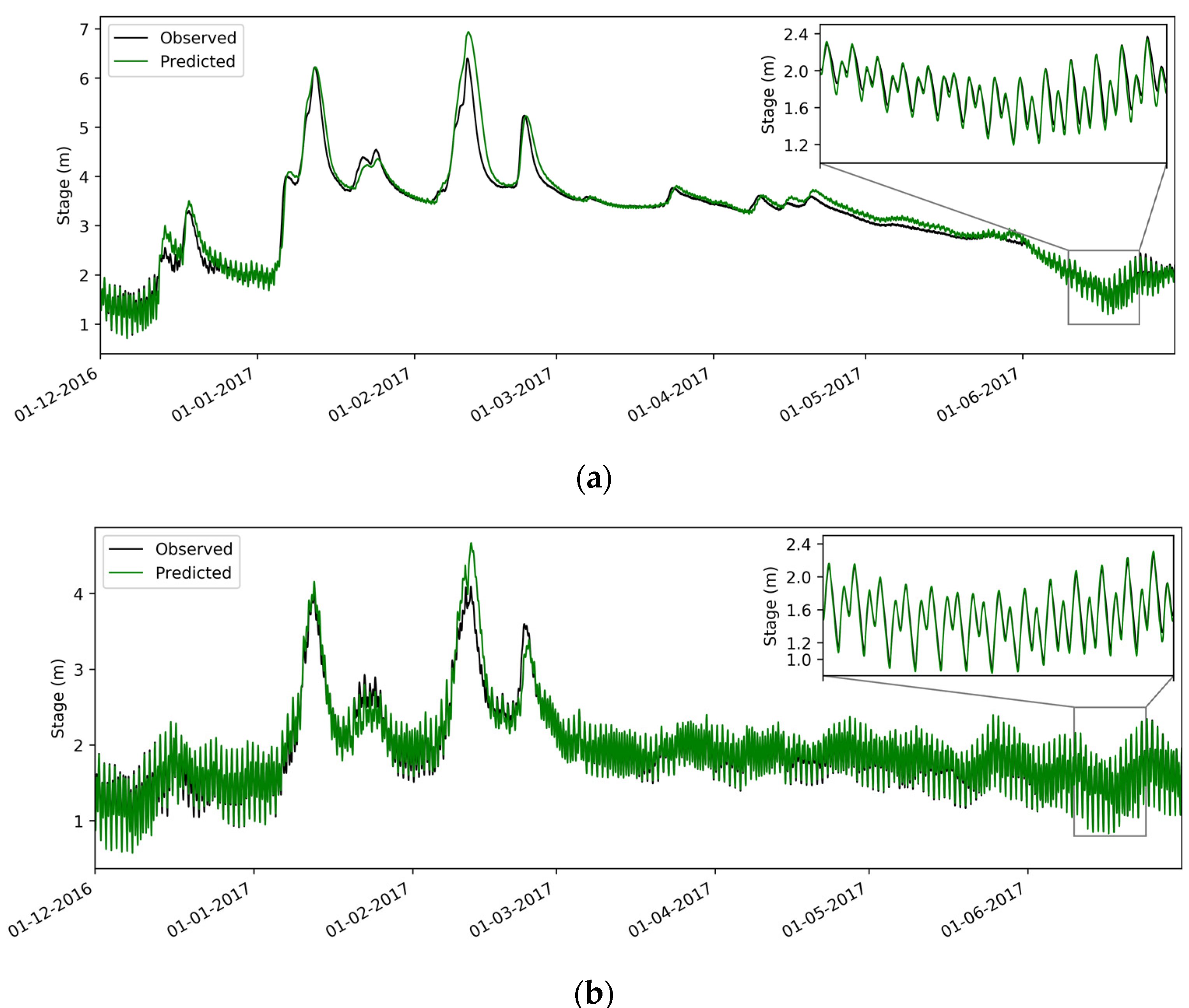
A 72-h model spin-up period was eliminated from the calibration metrics and plots due to the initial uniform water surface elevation being very low to ensure no water was initialized within the MWT ring levee. Figure 4 demonstrates model agreement with observations over time, along with a tidally dominant period in the inset to show resolution of the tidal regime.
2.3.4. Model Tracers
The UnTRIM modeling platform has the capacity to solve for the distribution of tracers with a transport scheme allowing for advection, diffusion, and source/sink terms. Conservative tracers were released within the model mesh and tracked across the domain with a horizontal diffusion coefficient of 0.0, considering only transport via advection using UnTRIM’s built-in transport solver [38]. The tracers act similarly to an inert dye and allow the model to follow the “traced” water throughout the model domain, allowing for tracking of SWF in space and time.
The vertically integrated transport equation for the tracers used is:
where is the concentration of the conservative scalar tracer. In this study we considered the numerical diffusion introduced by the model to be on the same order as that of physical diffusion processes and set the right hand side of Equation (7) was set to zero by using horizontal diffusion coefficients () of 0.0.
Throughout the simulation, tracers were released at the Cosumnes and Mokelumne Rivers with “Cosumnes” and “Mokelumne” tracers, corresponding to the C1 and M1 site locations, respectively. The tracers were released in all cells that spanned the rivers laterally at the locations where isotopes were collected for both rivers. An “Other” tracer was released at all flow boundaries and for all initial water. Upon passing through the Cosumnes release cells, the Mokelumne and Other tracers were set to zero. Similarly, for the Mokelumne release cells, the other and Cosumnes tracers were set to zero. After the simulation ran, the volumetric fractions of each individual tracer (Cosumnes, Mokelumne, and Other) were queried for each sample location (Figure 2) and checked to ensure that the sum of all three tracers was 1.0 over time, confirming mass balance in the transport model.
In this study, there was no field validation of the transport mechanisms. This is a limitation of the confidence in accuracy of the hydrodynamic approach, despite good hydraulic calibration.
3. Results
3.1. Isotope Mixing Model Results
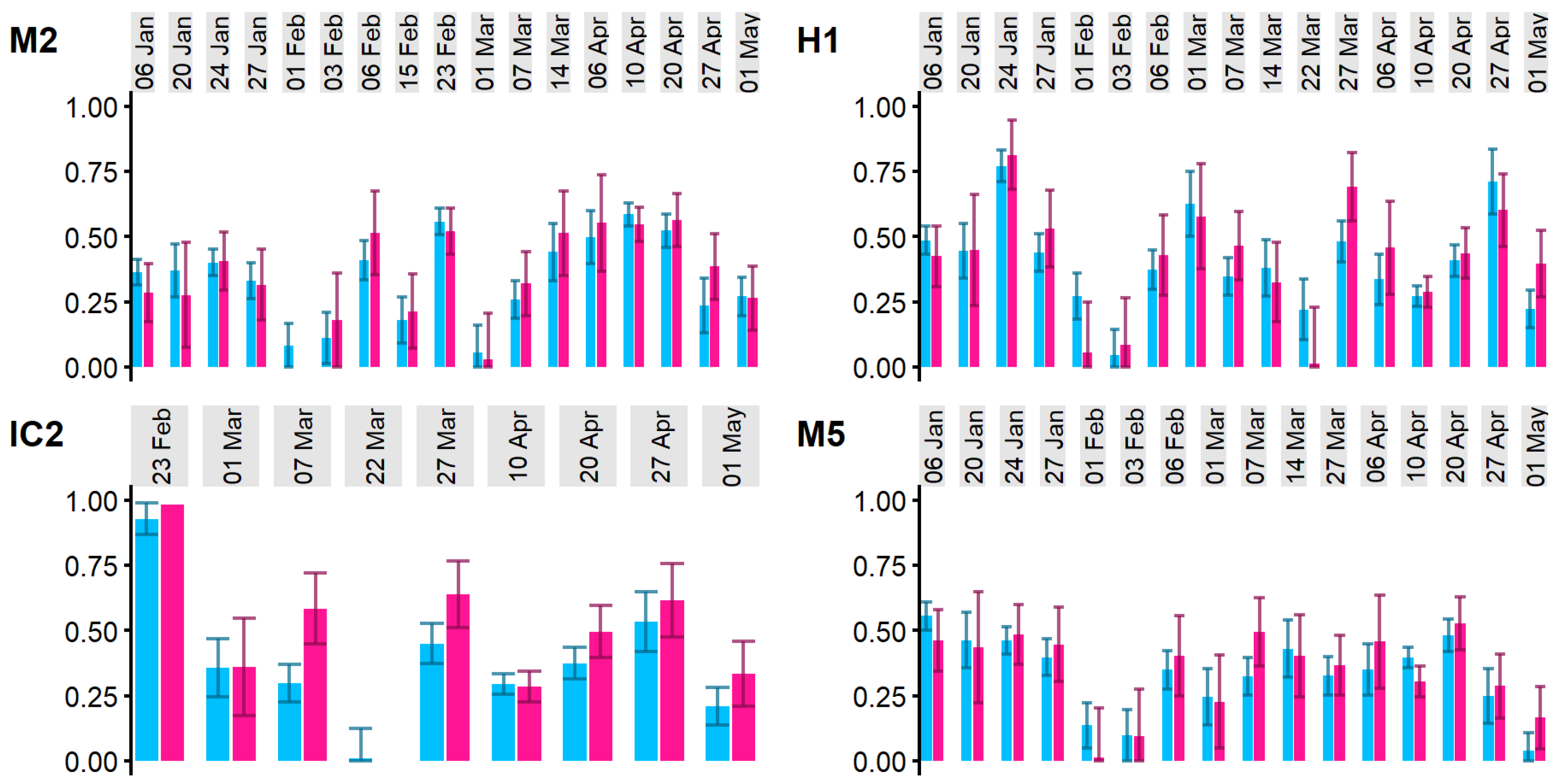
At each sample location and time, a mixing model was performed for both and ((Figure 5). With an instrument uncertainty of and for and , respectively, 95% confidence intervals were calculated from each mixing model result. The error bars were then calculated using the minimum and maximum error on each isotope value used in Equation (4). This calculation of instrument-derived error is the only measurable quantity of error that we addressed in this study due to the limitations associated with quantifying the error from breaking assumptions inherent in the mixing model. These assumptions include stationarity in the tributaries, local effects assumed to be negligible, and the sampled water was composed of only the two tributaries. At the time of sampling, only one water grab sample was taken for each site and date, meaning we were unable to compute a standard deviation in space or time of isotope composition at each site to accompany instrument error.
As shown in the Supplementary Table S1, differences between the C1 and M1 isotope values ranged from and for , and from and for . Given that the instrument error could account for anywhere from 5% to 51% of that range, the mixing model uncertainty ended up being quite significant (Figure 5).
Any isotopic values which did not lie between the C1 and M1 (Cosumnes and Mokelumne sample locations, respectively), were discarded as they would produce fractions larger than 1.0. Out of the 312 and mixing model results, only 13 were outside of the bounds set by the C1 and M1 values for those sample dates. After eliminating invalid data points, a total of 299 mixing model results were produced across 156 unique sample dates and times.
3.2. Hydrodynamic Tracer Results
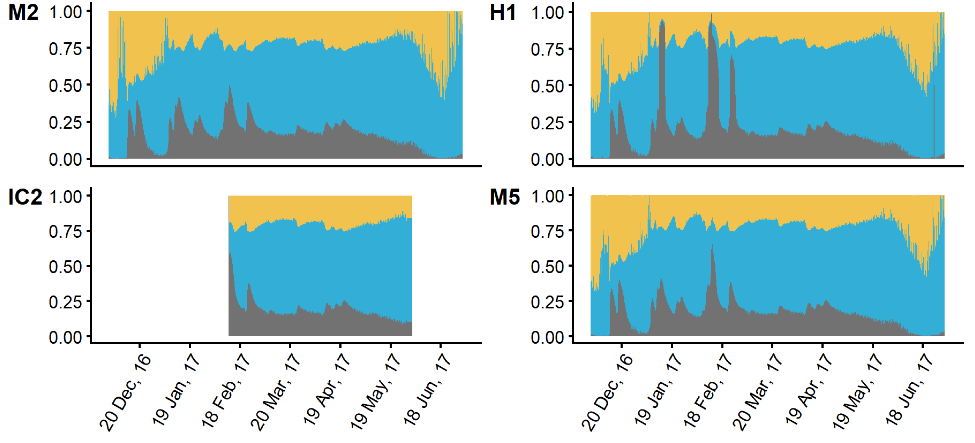
The model tracer simulation predicts the proportion of Cosumnes, Mokelumne, and Other tracers at the sample locations (Figure 6). The modeled distribution of tracers can also be displayed spatially for any moment in time during the simulation (Figure 7). The model produced time-varying SWF time series, where all tracers summed to one at all points in time, confirming mass conservation across all tracers. The time series demonstrate that over time, there is a trade-off of the three tracers, and that certain periods are dominated by a single tracer.
3.3. Mixing Model and Hydrodynamic Model Comparison
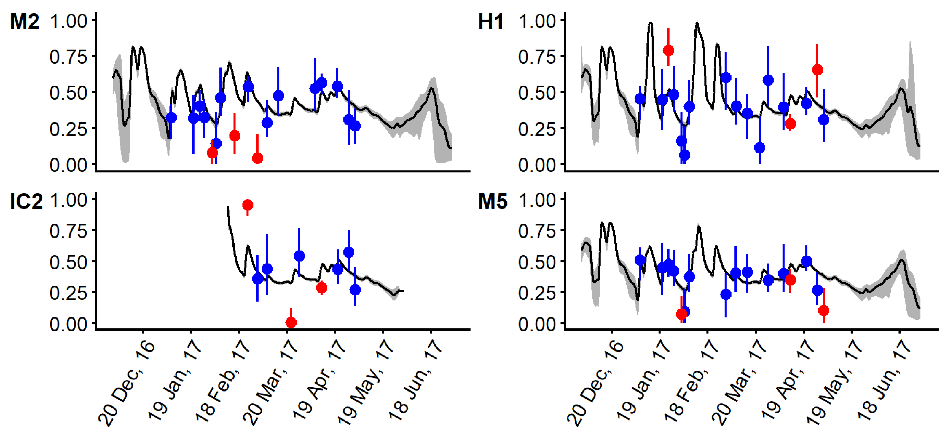
In comparing the difference between the model tracer-based estimation of source water versus the isotope mixing model approach (Figure 8), we assume the “Other” tracer would have a similar isotopic signature to the sample taken at the Cosumnes (C1, Figure 2) sample location. This is potentially due to the fact that the Cosumnes and its nearby tributaries (Deer Creek, Upper and Lower Laguna Creek, and Dry Creek) all have watersheds at similar elevations and inland extents to the Cosumnes watershed; presumably, these waterways would receive precipitation of a similar isotopic composition. Furthermore, the water within the channel at the Cosumnes sample location is a continuation of the larger pulses of floodwaters coming through the Cosumnes River Floodplain following rain events, that would be considered “Other” by the hydrodynamic approach. Because of this assumption, we use the combined “Other” and “Cosumnes” tracer results to make a comparison with the averaged and mixing model results. Interestingly, this pattern of apparent isotopic similarity between the Cosumnes sample location and other water is consistent at the S1 and S2 sites (Figure 2), which have a significant amount of Snodgrass Slough water. That Snodgrass water was tagged as other in the model, as it is one of the flow boundaries where all water is tagged as other. Where the isotope mixing model predicts Cosumnes water, the hydrodynamic model output presents that fraction as a combination of other and Cosumnes water. This could be due to the source water for Snodgrass Slough (Morrison Creek) having similar watershed characteristics that lead to the isotope signature for the Cosumnes and its tributaries.
The hydrodynamic “Other” and “Cosumnes” tracers were combined into an instantaneous time series for each site, then the 12-h running mean, minima, and maxima were tidally averaged using a Godin filter to produce a tidal envelope to compare to the isotope mixing model results (Figure 8). At each site, there were varying degrees of overlap (Table 2), with only two sites (ISE and L1) (Figure 2) under 60%.
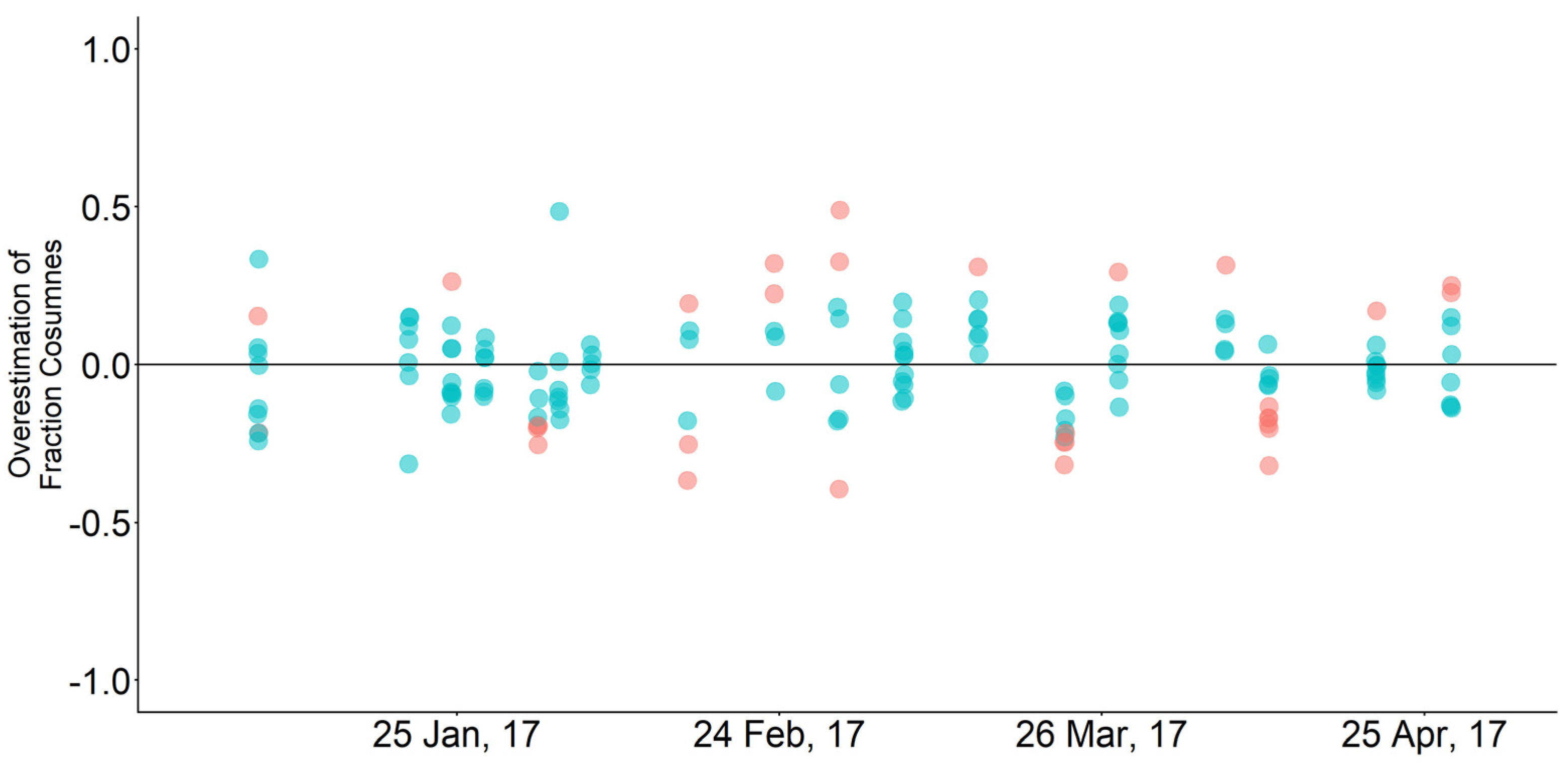
An overwhelming majority of the sites were considered overlapping in uncertainty, implying that both methods produced similar results within the bounds of their uncertainty (Figure 9). In total, 123 out of the 156 samples compared were considered overlapping (78.9% overall). Although the methods largely agreed, the isotopic results alone produced a good estimate with a lot of uncertainty from instrument error, while the hydrodynamic results provided improved accuracy, as well as finer spatiotemporal resolution.
4. Discussion and Conclusions
This study compared two techniques from two fields of study in order to arrive at estimates of source water fraction (SWF) within a natural system. The hydrodynamic model provided estimated flows and mixing patterns to complement a field-based isotope approach that would otherwise be unsubstantiated (as opposed to previous field-based studies [21,22]). Similarly, the isotope findings act as a field-validation for a numerically-based method of finding SWF in surface-water systems. Both methodologies can be applied to other riverine systems. In order to confidently use the isotope mixing model approach, one would want to ensure that the system is fluvially dominated, that each source tributary has a distinct isotopic signature, and that some stationarity exists in the isotope composition of those source waters [33]. Both methods provide insight to the larger issue of tracing the composition of water in a system in order to better understand the larger mixing processes and patterns in a complex river network. Inherent in the methods are a few assumptions.
Throughout the course of the 2017 sampling done for this paper, our river system was dominated by fluvial processes, unlike typical conditions in which the study area experiences a tidal signal. To compare to 2017, which was a wet year, we briefly compared the two SWF methods in 2018 and 2019 floods, which were below normal years, and found there was little agreement, likely because of the flows not being strong or persistent enough to maintain a fluvial character to the study site. During the 2017 period of this study, the two methods outlined produced similar results, despite the major assumption in the isotope mixing model () being imprecise due to widespread overland flow and the high “Other” fractions modeled at the sample sites. Presumably, an increased spatial extent for isotopic sampling could partially alleviate this limitation, although when the number of sources exceeds two, solutions to an expanded Equations (1), (8) and (9) become non-unique. There are additional limitations to the methodologies that may affect the validity of results.
The assumption that endpoint (C1 and M1) samples are representative of cross-sectional averaged isotopic composition may also be imprecise. At each of these locations one sample was collected at one location in the cross-section per sampling date. To evaluate the impacts of this limitation in single-sample field locations, we evaluated model output for all cells across the channel for sites M2, M3, and IA2 and found that the Cosumnes and Mokelumne River waters were well-mixed laterally at the time of sampling, indicating that the lack of replicate samples in the lateral did not necessarily present errors when compared to the model results. However, because this study was performed using a depth-averaged model we cannot investigate sensitivity to the water sample being taken near the top of the water column, but we can assume that the vertical mixing past the confluence is thorough [13]. Although the model accurately predicts cross-sectional flows and stage, the same issue arises as in the study on the model watershed by Peter et al. [22]: the exact flow and mixing patterns are unknown.
The calibrated hydrodynamic model coupled with a transport model provides more spatiotemporally specific output that has proven to be reliable within the bounds of the field data approach this study used. Additionally, the number of water sources traced is unlimited, unlike the isotope-based approach that is limited to two source tributaries. Another advantage of the hydrodynamic model approach over the isotope mixing model is there is no necessity for the source waters to be isotopically distinct. Lastly, the hydrodynamic model predicts additional variables such as depth and velocity that could provide habitat characteristic values (e.g., Pasternack et al. 2004 [39], Whipple 2018 [40]) to be combined with SWF results to further evaluate restoration potential.
Before exploring the significance of applications to other systems, let us explore the significance to the McCormack-Williamson Tract (MWT). There have been a few examples of multiple restoration sites along a river having cumulative benefits as one moves downstream. These have been demonstrated in gravel restoration sites along rivers in the Sacramento–San Joaquin River system [39,41,42], and the multitude of restoration sites across freshwater tributaries of the Chesapeake Bay [43] where restored sites along a river continuum act as a “string of pearls” of aquatic habitat. Ultimately, as water moves through rehabilitated habitat its ecological value or potential cumulatively improves [44,45] It follows that the restoration-laden Cosumnes River carries with it the potential to boost restoration value within the MWT restoration: the last “pearl” in the string. Understanding the spatiotemporal patterns of SWF allows us to identify regions that retain source waters from the Cosumnes, and thus water that has a higher likelihood to contain nutrients or productivity from upstream restoration sites [31,46,47]. Being downstream of completed and ongoing restoration projects is not a unique trait of the MWT within the Delta. Many restoration sites are slated or under construction in the Delta [48]. Understanding how these sites are connected and how they can be synergistic may help to better understand how a single site can have regional ecosystem benefits.
Given that the hydrodynamic method of finding SWF discussed in this paper could be applied to any river network, insights on riverine restoration potential can be gained in any system. For simple fluvial systems that satisfy the assumptions of the isotope mixing model method of finding SWF, isotope samples could suffice in place of developing hydrodynamic models. With careful regard for the limitations discussed, the implications for understanding SWF distribution can be further explored in any river network, and perhaps other connections to aquatic ecology or water quality processes can be found. For instance, Farly et al. used an isotope mixing model to investigate fish diet composition in terms of floodplain-produced or channel-produced resources [49]. This could be coupled with hydrodynamic models to investigate possible effects of drift versus autochthonous production. These methods (hydrodynamic tracers and isotope mixing models) can also be used to investigate habitat quality and its linkages to SWF, using a number of biological or water quality data.
Supplementary Materials
The following are available online at https://www.mdpi.com/2073-4441/12/4/1128/s1. Table S1: Field and isotope data for all sites.
Author Contributions
Conceptualization, B.N., C.J., and L.A.T.; Methodology, B.N., L.A.T., and E.S.G.; Supervision, C.J., E.S.G. and M.L.F.; Writing—original draft, L.T.; Writing—reviewing & editing, L.A.T., B.N., E.S.G., M.L.F., and C.J. All authors have read and agreed to the published version of the manuscript.
Funding
This research was funded by the Delta Stewardship Council, grant 1471.
Acknowledgments
Christopher “Rusty” Holleman for coding and modeling support, William “Bill” Fleenor for guidance and institutional knowledge on the MWT, Thomas Handley for bathymetric support, Fabián Bombardelli for advice and guidance in modeling and analysis, Alison Whipple for helping secure funding and for sharing hydrologic methods to develop boundary conditions, David Ford Engineering Consulting for the hydrologic work to support the boundary conditions, cbec eco engineering (especially Chris Campbell, Chris Hammersmark) for providing previous modeling work, and The Nature Conservancy for their support of the project that allowed this research to be possible.
Conflicts of Interest
The authors declare no conflict of interest.
References
- Day, J.W.; Hall, C.A.S.; Kemp, W.M.; Yanez-Arancibia, A. Estuarine Ecology, 2nd ed.; Day, J.W.J., Crump, B.C., Kemp, W.M., Yanez-Arancibia, A., Eds.; John Wiley & Sons, Inc.: Hoboken, NJ, USA, 1988. [Google Scholar] [CrossRef]
- Ruiz, G.M.; Carlton, J.T.; Grosholz, E.D.; Hines, A.H. Global invasions of marine and estuarine habitats by non-indigenous species: Mechanisms, extent, and consequences. Am. Zool. 1997, 37, 621–632. [Google Scholar] [CrossRef]
- Worm, B.; Barbier, E.B.; Beaumont, N.; Duffy, J.E.; Folke, C.; Halpern, B.S.; Jackson, J.B.C.; Lotze, H.K.; Micheli, F.; Palumbi, S.R.; et al. Impacts of Biodiversity Loss on Ocean Ecosystem Services. Science 2006, 314, 787–790. [Google Scholar] [CrossRef] [PubMed] [Green Version]
- Lotze, H.K.; Lenihan, H.S.; Bourque, B.J.; Bradbury, R.H.; Cooke, R.G.; Kay, M.C.; Kidwell, S.M.; Kirby, M.X.; Peterson, C.H.; Jackson, J.B.C. Depletion, degradation, and recovery potential of estuaries and coastal seas. Science 2006, 312, 1806–1809. [Google Scholar] [CrossRef] [PubMed]
- Bowen, J.L.; Valiela, I. The ecological effects of urbanization of coastal watersheds: Historical increases in nitrogen loads and eutrophication of Waquoit Bay estuaries. Can. J. Fish. Aquat. Sci. 2001, 58, 1489–1500. [Google Scholar] [CrossRef]
- Kuivila, K.; Hladik, M.L. Understanding the occurrence and transport of current-use pesticides in the San Francisco estuary watershed. San Fr. Estuary Watershed Sci. 2008, 6. [Google Scholar] [CrossRef] [Green Version]
- Hong, B.; Shen, J. Responses of estuarine salinity and transport processes to potential future sea-level rise in the Chesapeake Bay. Estuar. Coast. Shelf Sci. 2012, 104–105, 33–45. [Google Scholar] [CrossRef]
- Nilsson, C.; Reidy, C.A.; Dynesius, M.; Revenga, C. Fragmentation and flow regulation of the world’s large river systems. Science 2005, 308, 405–408. [Google Scholar] [CrossRef] [Green Version]
- Drinkwater, K.F. On the Role of Freshwater Outflow on Coastal Marine Ecosystems—A Workshop Summary. In The Role of Freshwater Outflow in Coastal Marine Ecosystems; Skreslet, S., Ed.; Springer: Berlin/Heidelberg, Germany, 1986; pp. 429–438. [Google Scholar]
- Whipple, A.A.; Grossinger, R.M.; Rankin, D.; Stanford, B.; Askevold, R.A. Sacramento-San Joaquin Delta Historical Ecology Investigation: Exploring Pattern and Process; SFEI Contribution No. 672; San Francisco Estuary Institute-Aquatic Science Center: Richmond, CA, USA, 2012. [Google Scholar]
- Dahl, T.E.; Allord, G.J. Technical Aspects of Wetlands: History of Wetlands in the Conterminous United States; United States Geological Survey Water Supply Paper 2425; US Geological Survey: Reston, VA, USA, 1996.
- Ahearn, D.S.; Viers, J.H.; Mount, J.F.; Dahlgren, R.A. Priming the productivity pump: Flood pulse driven trends in suspended algal biomass distribution across a restored floodplain. Freshw. Biol. 2006, 51, 1417–1433. [Google Scholar] [CrossRef]
- Fischer, H.B.; List, E.J.; Koh, R.C.Y.; Imberger, J.; Brooks, N.H. Mixing in Inland and Coastal Waters; Academic Press: San Diego, CA, USA, 1979. [Google Scholar]
- Gibson, J.J.; Reid, R. Water balance along a chain of tundra lakes: A 20-year isotopic perspective. J. Hydrol. 2014, 519, 2148–2164. [Google Scholar] [CrossRef]
- Sherman, L.S.; Blum, J.D.; Dvonch, J.T.; Gratz, L.E.; Landis, M.S. The use of Pb, Sr, and Hg isotopes in great lakes precipitation as a tool for pollution source attribution. Sci. Total Environ. 2015, 502, 362–374. [Google Scholar] [CrossRef]
- Krabbenhoft, D.P.; Bowser, C.J.; Kendall, C.; Gat, J.R. Use of oxygen-18 and deuterium to assess the hydrology of groundwater-lake systems. Environ. Chem. Lakes Reserv. 1994, 90. [Google Scholar] [CrossRef]
- Vitvar, T.; Burns, D.A.; Lawrence, G.B.; Mcdonnell, J.J.; Wolock, D.M. Estimation of baseflow residence times in watersheds from the runoff hydrograph recession: Method and application in the Neversink Watershed, Catskill Mountains, New York. Hydrol. Process. 2002, 16, 1871–1877. [Google Scholar] [CrossRef]
- Marchina, C.; Bianchini, G.; Natali, C.; Pennisi, M.; Colombani, N.; Tassinari, R.; Knoeller, K. The Po river water from the Alps to the Adriatic Sea (Italy): New insights from geochemical and isotopic (Δ18O-ΔD) data. Environ. Sci. Pollut. Res. 2015, 22, 5184–5203. [Google Scholar] [CrossRef] [PubMed]
- Penna, D.; Zuecco, G.; Crema, S.; Trevisani, S.; Cavalli, M.; Pianezzola, L.; Marchi, L.; Borga, M. Response time and water origin in a steep nested catchment in the Italian dolomites. Hydrol. Process. 2017, 31, 768–782. [Google Scholar] [CrossRef]
- Marchina, C.; Lencioni, V.; Paoli, F.; Rizzo, M.; Bianchini, G. Headwaters’ isotopic signature as a tracer of stream origins and climatic anomalies: Evidence from the Italian Alps in summer 2018. Water 2020, 12, 309. [Google Scholar] [CrossRef] [Green Version]
- Halder, J.; Decrouy, L.; Vennemann, T.W. Mixing of Rhône River water in Lake Geneva (Switzerland–France) inferred from stable hydrogen and oxygen isotope profiles. J. Hydrol. 2013, 477, 152–164. [Google Scholar] [CrossRef]
- Peter, K.T.; Wu, C.; Tian, Z.; Kolodziej, E.P. Application of nontarget high resolution mass spectrometry data to quantitative source apportionment. Environ. Sci. Technol. 2019, 53, 12257–12268. [Google Scholar] [CrossRef]
- Sridharan, V.K.; Monismith, S.G.; Fong, D.A.; Hench, J.L. One-dimensional particle tracking with streamline preserving junctions for flows in channel networks. J. Hydraul. Eng. 2018, 144, 1–10. [Google Scholar] [CrossRef]
- Bai, H.; Chen, Y.; Wang, D.; Zou, R.; Zhang, H.; Ye, R.; Ma, W.; Sun, Y. Developing an EFDC and numerical source-apportionment model for nitrogen and phosphorus contribution analysis in a lake basin. Water 2018, 10, 1315. [Google Scholar] [CrossRef] [Green Version]
- Lund, J.R. Envisioning Futures for the Sacramento-San Joaquin Delta; Public Policy Institute of California: San Francisco, CA, USA, 2007. [Google Scholar]
- Mount, J.; Bennett, W.; Durand, J.; Fleenor, W.; Hanak, E.; Lund, J.; Moyle, P. Aquatic Ecosystem Stressors in the Sacramento–San Joaquin Delta; The Public Policy Institute of California (PPIC): San Francisco, CA, USA, 2012. [Google Scholar]
- Gross, E.S.; Hutton, P.H.; Draper, A.J. A comparison of outflow and salt intrusion in the pre-development and contemporary San Francisco Estuary. San Fr. Estuary Watershed Sci. 2018, 16. [Google Scholar] [CrossRef] [Green Version]
- Lund, J.; Hanak, E.; Fleenor, W.; Bennett, W.; Howitt, R.; Mount, J.; Moyle, P. Comparing Futures for the Sacramento-San Joaquin Delta; University of California Press: Berkely, CA, USA, 2010. [Google Scholar]
- Moyle, P.B.; Crain, P.K.; Whitener, K. Patterns in the use of a restored california floodplain by native and alien fishes. San Fr. Estuary Watershed Sci. 2007, 5, 1–29. [Google Scholar] [CrossRef]
- Brown, K.J.; Pasternack, G.B. The geomorphic dynamics and environmental history of an upper deltaic floodplain tract in the Sacramento-San Joaquin Delta, California, USA. Earth Surf. Process. Landforms 2004, 29, 1235–1258. [Google Scholar] [CrossRef]
- Whipple, A.A.; Viers, J.H.; Dahlke, H.E. Flood regime typology for floodplain ecosystem management as applied to the unregulated Cosumnes River of California, United States. Ecohydrology 2017, 10, 1–18. [Google Scholar] [CrossRef] [Green Version]
- Jeffres, C.A.; Opperman, J.J.; Moyle, P.B. Ephemeral floodplain habitats provide best growth conditions for juvenile Chinook salmon in a California River. Environ. Biol. Fishes 2008, 83, 449–458. [Google Scholar] [CrossRef]
- Gat, J.R. Oxygen and hydrogen isotopes in the hydrologic cycle. Annu. Rev. Earth Planet. Sci. 1996, 24, 225–262. [Google Scholar] [CrossRef] [Green Version]
- Casulli, V.; Walters, R.A. An unstructured grid, three-dimensional model based on the shallow water equations. Int. J. Numer. Methods Fluids 2000, 32, 331–348. [Google Scholar] [CrossRef]
- Walters, R.A.; Casulli, V. A robust, finite element model for hydrostatic surface water flows. Commun. Numer. Methods Eng. 1998, 14, 931–940. [Google Scholar] [CrossRef]
- David Ford Consulting Engineers. Cosumnes and Mokelumne River Watersheds—Design Storm Runoff Analysis; David Ford Consulting Engineers: Sacramento, CA, USA, 2004. [Google Scholar]
- Willmott, C.J. On the validation of models. Phys. Geogr. 1981, 2, 184–194. [Google Scholar] [CrossRef]
- Casulli, V.; Zanolli, P. Semi-implicit numerical modeling of nonhydrostatic free-surface flows for environmental problems. Math. Comput. Model. 2002, 36, 1131–1149. [Google Scholar] [CrossRef]
- Pasternack, G.B.; Wang, C.L.; Merz, J.E. Application of a 2D hydrodynamic model to design of reach-scale spawning gravel replenishment on the Mokelumne River, California. River Res. Appl. 2004, 20, 205–225. [Google Scholar] [CrossRef]
- Whipple, A.A. Managing Flow Regimes and Landscapes Together: Hydrospatial Analysis for Evaluating Spatiotemporal Floodplain Inundation Patterns with Restoration and Climate Change Implications. Ph.D. Thesis, University of California, Davis, CA, USA, June 2018. [Google Scholar]
- Kondolf, G.M.; Angermeier, P.L.; Cummins, K.; Dunne, T.; Healey, M.; Kimmerer, W.; Moyle, P.B.; Murphy, D.; Patten, D.; Railsback, S.; et al. Projecting cumulative benefits of multiple river restoration projects: An example from the Sacramento-San Joaquin River System in California. Environ. Manag. 2008, 42, 933–945. [Google Scholar] [CrossRef] [PubMed]
- Parker, S.S.; Remson, E.J.; Verdone, L.N. Restoring conservation nodes to enhance biodiversity and ecosystem function along the Santa Clara River. Ecol. Restor. 2014, 32, 6–8. [Google Scholar] [CrossRef]
- Hassett, B.; Palmer, M.; Bernhardt, E.; Smith, S.; Carr, J.; Hart, D. Restoring watersheds project by project: Trends in Chesapeake Bay tributary restoration. Front. Ecol. Environ. 2005, 3, 259–267. [Google Scholar] [CrossRef]
- Vannote, R.L.; Minshall, G.W.; Cummins, K.W.; Sedell, J.R.; Cushing, C.E. The river continuum concept. Can. J. Fish. Aquat. Sci. 1980, 37, 130–137. [Google Scholar] [CrossRef]
- Palmer, M.A.; Bernhardt, E.S.; Allan, J.D.; Lake, P.S.; Alexander, G.; Brooks, S.; Carr, J.; Clayton, S.; Dahm, C.N.; Follstad Shah, J.; et al. Standards for ecologically successful river restoration. J. Appl. Ecol. 2005, 42, 208–217. [Google Scholar] [CrossRef]
- Swenson, R.O.; Whitener, K.; Eaton, M. Restoring floods on floodplains: Riparian and floodplain restoration at the Cosumnes River Preserve. In California Riparian Systems: Processes and Floodplain Management, Ecology and Restoration; Riparian Habitat Joint Venture: Sacramento, CA, USA, 2003; pp. 224–229. [Google Scholar]
- Opperman, J.J.; Luster, R.; McKenney, B.A.; Roberts, M.; Meadows, A.W. Ecologically functional floodplains: Connectivity, flow regime, and scale. J. Am. Water Resour. Assoc. 2010, 46, 211–226. [Google Scholar] [CrossRef]
- California Natural Resources Agency; California Department of Food and Agriculture; California Environmental Protection Agency. California Water Action Plan: 2016 Update; California Natural Resources Agency: Sacramento, CA, USA; California Department of Food and Agriculture: Sacramento, CA, USA; California Environmental Protection Agency: Sacramento, CA, USA, 2016.
- Farly, L.; Hudon, C.; Cattaneo, A.; Cabana, G. Seasonality of a floodplain subsidy to the fish community of a large temperate river. Ecosystems 2019, 22, 1823–1837. [Google Scholar] [CrossRef]
Figure 1.
Study area with calibration gage stations shown as black points. Sensors deployed specifically for this study are triangles, and agency gages (either United States Geological Survey (USGS) or the California Department of Water Resources (DWR)) are squares. The model domain is shown (bottom right, location shown as red dot in California) overlying the Delta waterways in blue. Boundary gages are shown in the bottom right figure with agency gages shown as white and black icons and estimated boundaries labeled with blue arrows.

Figure 2.
Study area showing isotope sample locations in white, with the Cosumnes and Mokelumne Base locations shown in orange and blue, respectively.
Figure 2.
Study area showing isotope sample locations in white, with the Cosumnes and Mokelumne Base locations shown in orange and blue, respectively.

Figure 3.
Schematic river system with single confluence.

Figure 4.
Calibration plot for the BEN (a), and SMR (b) gages (Table 1) showing the observed (black) and modeled (green) water surface elevation for the period simulated. The inset shows the comparison of observed versus modeled during a tidally dominated period.
Figure 4.
Calibration plot for the BEN (a), and SMR (b) gages (Table 1) showing the observed (black) and modeled (green) water surface elevation for the period simulated. The inset shows the comparison of observed versus modeled during a tidally dominated period.

Figure 5.
Isotope mixing model results showing fraction of Cosumnes on the y-axis for (blue) and (pink), along with instrument error bars at four example locations (depicted in Figure 3) in 2017. M2 Downstream of confluence. H1: Dead Horse Cut. IC2: Island site C2. M5: South Fork Mokelumne.
Figure 5.
Isotope mixing model results showing fraction of Cosumnes on the y-axis for (blue) and (pink), along with instrument error bars at four example locations (depicted in Figure 3) in 2017. M2 Downstream of confluence. H1: Dead Horse Cut. IC2: Island site C2. M5: South Fork Mokelumne.

Figure 6.
Source water fraction time series at four example locations (depicted in Figure 3) where all fractions add to 1.0. The yellow portion represents the Cosumnes tracer, the blue portion represents the Mokelumne tracer, and the grey represents the other tracer. M2: Downstream of confluence. H1: Dead Horse Cut. IC2: Island site C2. M5: South Fork Mokelumne.

Figure 7.
Mapping of the distribution of the three numerical tracers within the model domain. The Cosumnes tracer is shown in orange (A), the Mokelumne tracer is blue (B), and the other tracer is shown in black/grey (C). The snapshot is at 12 February, 2017 02:30, and demonstrates how the Cosumnes and Mokelumne tracers are released and transported downstream (leftwards).

Figure 8.
Time series at four locations showing the modeled Cosumnes and Other concentrations with the tidal average (black line) and tidal envelope (grey ribbon). The isotope mixing model values are shown as points with the isotope instrument 95% confidence intervals extending from the mixing model value. Blue points are those whose isotopic confidence intervals overlap with the modeled tidal envelope, while red points do not.

Figure 9.
Time series of all locations with overestimation of the fraction Cosumnes found in the isotope method versus the hydrodynamic model method. The blue dots represent sample points whose uncertainty overlapped with the tidal envelope of the model results, and the red dots did not overlap (as in Figure 8).


Table 1.
Model calibration metrics for the gages shown in Figure 2.
Table 1.
Model calibration metrics for the gages shown in Figure 2.
| Gage Name | Gage ID * | R2 | Skill | Date Range | |
|---|---|---|---|---|---|
| Stage | Mokelumne R @ Benson’s Ferry NR Thornton | BEN C | 0.976 | 0.991 | 1 December 2016–1 July 2017 |
| Delta Cross Channel BTW Sac R & Snodgrass | DLC U | 0.963 | 0.989 | 1 December 2016–1 July 2017 | |
| Sacramento River Below Georgiana Slough | GES U | 0.977 | 0.99 | 1 December 2016–1 July 2017 | |
| Georgiana Slough at Sacramento River | GSS U | 0.976 | 0.989 | 1 December 2016–1 July 2017 | |
| Middle Slough | MSL L | 0.959 | 0.986 | 20 January 2017–1 July 2017 | |
| McCormack-Williamson Tract – Inlet | MTI L | 0.932 | 0.974 | 16 February 2017–31 May 2017 | |
| McCormack-Williamson Tract – Lower | MTL L | 0.914 | 0.976 | 16 February 2017–31 May 2017 | |
| North Mokelumne R at W Walnut Grove Rd | NMR U | 0.985 | 0.996 | 1 December 2016–1/11/2017 | |
| South Mokelumne R at W Walnut Grove Rd | SMR U | 0.969 | 0.99 | 1 December 2016–1 July 2017 | |
| Snodgrass Slough Upstream of Meadow | SUM L | 0.922 | 0.979 | 1 January 2017–1 July 2017 | |
| Flow | Sacramento River Below Georgiana Slough | GES U | 0.993 | 0.997 | 1 December 2016–1 July 2017 |
| Georgiana Slough at Sacramento River | GSS U | 0.974 | 0.973 | 1 December 2016–1 July 2017 | |
| South Mokelumne R at W Walnut Grove Rd | SMR U | 0.914 | 0.965 | 1 December 2016–1 July 2017 | |
| North Mokelumne R at W Walnut Grove Rd | NMR U | 0.958 | 0.98 | 1 December 2016–11 January 2017 |
* Gage data sources are denoted as C—DWR, U—USGS gage, L—LevelLogger sensor deployed for this study.
Table 2.
Summary statistics for each site (Figure 2) showing the percentage of points overlapping as well as the count.
Table 2.
Summary statistics for each site (Figure 2) showing the percentage of points overlapping as well as the count.
| Site | Total Samples | Overlapping Samples | Percentage Overlapping Samples |
|---|---|---|---|
| D1 | 5 | 8 | 82.4% |
| H1 | 14 | 17 | 62.5% |
| IA2 | 9 | 11 | 82.4% |
| IC2 | 6 | 9 | 81.8% |
| ID2 | 1 | 1 | 66.7% |
| IDC | 8 | 11 | 100.0% |
| INB | 1 | 2 | 72.7% |
| ISE | 4 | 10 | 50.0% |
| L1 | 10 | 11 | 40.0% |
| L2 | 8 | 9 | 90.9% |
| M2 | 14 | 17 | 75.0% |
| M3 | 16 | 17 | 88.9% |
| M4 | 6 | 8 | 94.1% |
| M5 | 13 | 16 | 83.3% |
| S1 | 5 | 6 | 100.0% |
© 2020 by the authors. Licensee MDPI, Basel, Switzerland. This article is an open access article distributed under the terms and conditions of the Creative Commons Attribution (CC BY) license (http://creativecommons.org/licenses/by/4.0/).
Share and Cite
MDPI and ACS Style
Tomkovic, L.A.; Gross, E.S.; Nakamoto, B.; Fogel, M.L.; Jeffres, C. Source Water Apportionment of a River Network: Comparing Field Isotopes to Hydrodynamically Modeled Tracers. Water 2020, 12, 1128. https://doi.org/10.3390/w12041128
AMA Style
Tomkovic LA, Gross ES, Nakamoto B, Fogel ML, Jeffres C. Source Water Apportionment of a River Network: Comparing Field Isotopes to Hydrodynamically Modeled Tracers. Water. 2020; 12(4):1128. https://doi.org/10.3390/w12041128
Chicago/Turabian StyleTomkovic, Lily A., Edward S. Gross, Bobby Nakamoto, Marilyn L. Fogel, and Carson Jeffres. 2020. "Source Water Apportionment of a River Network: Comparing Field Isotopes to Hydrodynamically Modeled Tracers" Water 12, no. 4: 1128. https://doi.org/10.3390/w12041128
Note that from the first issue of 2016, this journal uses article numbers instead of page numbers. See further details here.