Identification of the Nitrogen Sources in the Eocene Aquifer Area (Palestine)


1
Department of Civil Engineering, College of Engineering, An-Najah National University, Nablus P.O. Box: 7, Palestine
2
Water and Environmental Studies Institute, An-Najah National University, Nablus P.O. Box: 7, Palestine
*
Author to whom correspondence should be addressed.
Water 2020, 12(4), 1121; https://doi.org/10.3390/w12041121
Submission received: 26 January 2020
/
Revised: 6 April 2020
/
Accepted: 7 April 2020
/
Published: 14 April 2020
(This article belongs to the Section Water Resources Management, Policy and Governance)
Abstract
:Groundwater is the main source of water in many countries all over the world. Prevention of the pollution of this source is essential for a sustainable utilization. Nitrate pollution of groundwater is a common problem due to the association between intensive agriculture to achieve food security and fertilization. For an efficient management of groundwater pollution from nitrate, the first step would be to quantify the different sources of nitrogen in the aquifer of concern. This paper aims at demonstrating a general approach based on Geographic Information Systems (GIS) to characterize the spatial distribution of the nitrogen amounts in the area of the Eocene aquifer (Palestine). The aquifer is heavily utilized for agricultural and domestic water supply. Fertilization in the study area is a widespread practice. As a result, the aquifer is undergoing a nitrate pollution problem. The methodology relies mainly on specifying all the sources of nitrogen in the aquifer area using GIS to account for spatiality. Thereafter, GIS attribute tables and Excel spreadsheets were utilized to quantify the magnitudes of nitrogen from the different sources. Maps of the corresponding on-ground nitrate, ammonium, organic nitrogen and total nitrogen were developed for the study area. The results indicate that the total on-ground annual nitrogen loading in the study area is about 3260 tons of which 38% is attributed to fertilizers (chemical and manure) where the dominant form of nitrogen is NH4 (58.3%). The average total on-ground nitrogen loading is 7028 kg-N/km2·year. The estimated annual nitrate leaching to the aquifer is 1968 kg-N/km2. The areas of high sources of nitrogen have long-term impacts on the degradation of the water quality of the aquifer. It is therefore essential to build up on the outcomes of this work and to develop a nitrate fate and transport model for the Eocene aquifer. This model will enable the stakeholders to arrive at the efficient alternatives to manage the nitrate contamination of the aquifer.
Keywords:
groundwater; nitrate; nitrogen; pollution; fertilizers; manure; leaching; Eocene; Palestine1. Introduction
Groundwater is the main source of water for the Palestinians living in the West Bank and Gaza Strip where 90% of the water supply comes from this resource [1]. Currently, the increasing population in Palestine places an on-going stress on the groundwater resources [2]. The situation is further exacerbated when considering the widespread intensive agricultural practices that are taking place in the study area and elsewhere in the West Bank and Gaza Strip. This described situation entails a double drawback as in the one hand the competitive use caused a quantity problem while in the other hand the agricultural practices had led to quality deterioration [1,3,4]. Generally, the elevated nitrate concentrations in the groundwater of the West Bank and Gaza Strip are of increasing concern [5,6,7,8,9,10,11,12,13,14,15]. This situation of nitrate pollution in the groundwater is an on-going issue in the Eocene aquifer (Palestine).
The Eocene aquifer (648 km2) provides water to ~200 thousands persons and supplies water for a wide range of agricultural activities. Many studies have highlighted the decline in water storage and the elevated nitrate concentrations in the aquifer [5,6]. This alarming situation in the aquifer has prompted the necessity to manage the extraction amounts and to control the nitrate pollution. Along with the agricultural activities that prevail in the area of the Eocene aquifer, there are many other sources that contribute to the nitrate pollution problem. These sources include the disposal of untreated wastewater and the use of contaminated water in irrigation along with other sources that are characterized by being point and non-point in nature [5].
Many studies in the literature have demonstrated different approaches to tackle the issue of groundwater pollution from nitrate [5,16,17,18,19,20]. In many cases, the emphasis was on the control of the on-ground nitrogen loading from the different manageable sources in order to reduce the nitrate occurrence in the groundwater by reducing the nitrate leaching from the unsaturated zone [19,21,22,23,24,25]. However, a subset of these studies had employed groundwater fate and transport models of nitrate in order to assess the adequacy and efficiency of the control/reduction of the magnitudes of the nitrogen sources on the nitrate levels in groundwater [21,26,27,28,29,30].
The quantification of the on-ground nitrogen amounts from the different sources is common between all the aforementioned studies. Nevertheless, this was tackled in different ways and approaches [25,31,32,33]. There are studies that demonstrated the spatiality and magnitudes of the on-ground nitrogen loadings and corresponding nitrate leaching to groundwater in order to facilitate the development of groundwater fate and transport models. These models can be based on governing equations of nitrate fate and transport [30,34,35,36] or based on artificial intelligence for instance [37,38] or statistical models [31].
This manuscript describes in detail the methodology for the computation of the spatial distribution of the on-ground nitrogen amounts in the area of the Eocene aquifer. It provides a realistic and practical implementation of the methodology. This work is an important one since it addresses the nitrate pollution in groundwater which is a concern in many aquifers worldwide. The quantification of the nitrogen sources entails a large number of parameters and this manuscript illustrates the key calculations and provides a pool of data that can be used elsewhere in situations of similar conditions. The plausibility of this work relies on the fact that any modeling work of nitrate fate and transport in groundwater entails the spatial distribution of the nitrate leaching which in turn relies chiefly on the sources of nitrogen and their corresponding magnitudes [21]. This work provides a map of the total nitrogen amounts from the different on-ground sources. This enables the determination of the areas of elevated nitrogen loadings and by having information regarding the groundwater flow direction and path lines to wells it will be possible to clarify why certain wells show elevated nitrate concentrations. This is quite possible by the fact that this work takes into consideration the spatiality of the sources in the study area. This spatiality is attributed to the on-ground practices that differ from place to another and vary in strength from location to location. This spatiality is well addressed by different means and tools including GIS data, land use classes and orthophotos.
When eventually considering the potential use of physically-based highly-distributed groundwater models then the adopted approach in this work will best suite these kinds of models especially when considering the use of MODFLOW and MT3DMS. However, an alternative approach would be to consider an overall lumped value for the nitrogen loading without highlighting its spatial distribution (see for instance [39,40]). The lumped parameter models are simple to develop and easy to implement. Yet, lumped parameter models will not realistically represent the source distribution. Thus, when spatiality is of upmost importance these models will not be the right choice.
This manuscript addresses the issue of the nitrogen sources in the area of the Eocene aquifer for the first time. In addition, the extent of the nitrogen sources and amounts in the study area are now fully identified and quantified. The computations are in general customized to the land use map and this enables the implementation of the methodology for other areas in Palestine. Although the main outcome of this work is a map that shows the spatial distribution of the total nitrogen from the different sources, yet there are many other outputs that are worth to mention including the basic statistics related to the different sources of nitrogen and their corresponding percentages of occurrence. The map of the loadings of the nitrogen sources can be utilized to direct the decision makers to the proper locations for implementing the potential management options that target the study area of the Eocene aquifer. In addition, the nitrogen loading map was utilized in determining the nitrate leaching to groundwater and thus this will aid in the development of the distributed groundwater fate and transport model of nitrate when needed. The entire work furnished in this paper was developed and presented in a manner that can be easily replicated.
2. Materials and Methods
2.1. General Description of the Study Area
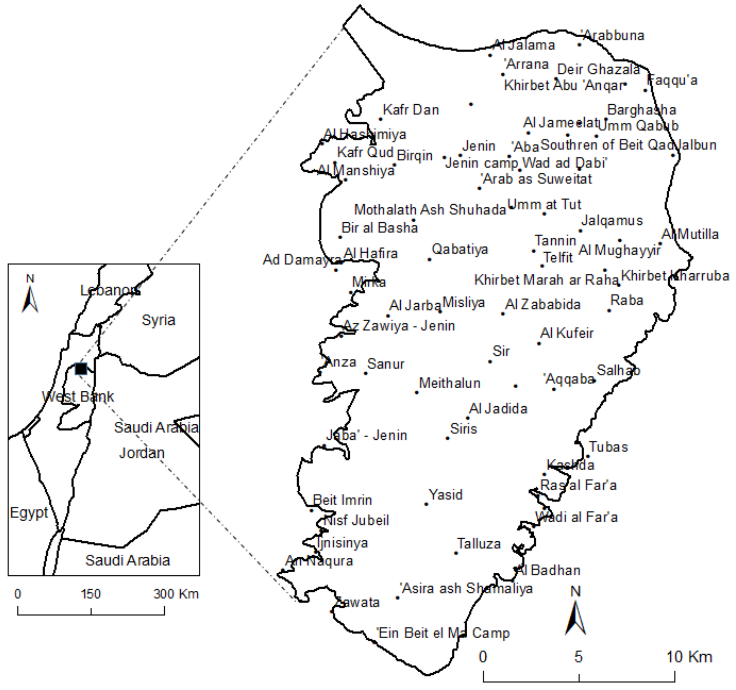
The Eocene aquifer is located in the northern part of the West Bank, Palestine (see Figure 1) and supplies water to the Palestinians for different uses [9,41]. It has a total area of about 648 km2 of which 463 km2 is within the West Bank, Palestine. The aquifer serves 43 communities with a total population of about 203,400 persons [42].
Rainfall varies throughout the study area where the annual rainfall is between 400 mm and 600 mm [43] with a general increasing trend toward the west and south. The study area can be classified as hot and dry during the summer and cool and wet in winter [44]. In winter, the minimum temperature is around 7 °C and the maximum is 15 °C. In summer, the average maximum temperature is 33 °C and the average minimum is 20 °C. Towards the west, the rate of potential evaporation decreases. The average annual potential evaporation ranges from 1850 mm to 2100 mm. The average annual relative humidity is around 62%. The soil types of the study area are Terra Rossa, Mediterranean Brown Forest Soils, Alluvial Soils, Colluvial-Alluvial Soils and Brown Alluvial Soils covering 49%, 16%, 14%, 13%, and 8% of the study area, respectively. The ground surface elevations in the study area range from 100 m above mean sea level (amsl) in the north to 925 m amsl in the south over a distance of approximately 35 km.
The geologic cross section of the study area shows the following formations arranged from oldest to youngest; limestone, dolomite and marl of Cenomanian to Turonian age, chalk and chert of Senonian age, chalk, limestone and chert of Eocene age and alluvium of Pleistocene [45]. However, the Eocene aquifer overlies the upper Cenomanian-Turnoian aquifer, with a transition zone of chalk and chert that varies in its thickness from 0 to 480 m [46].
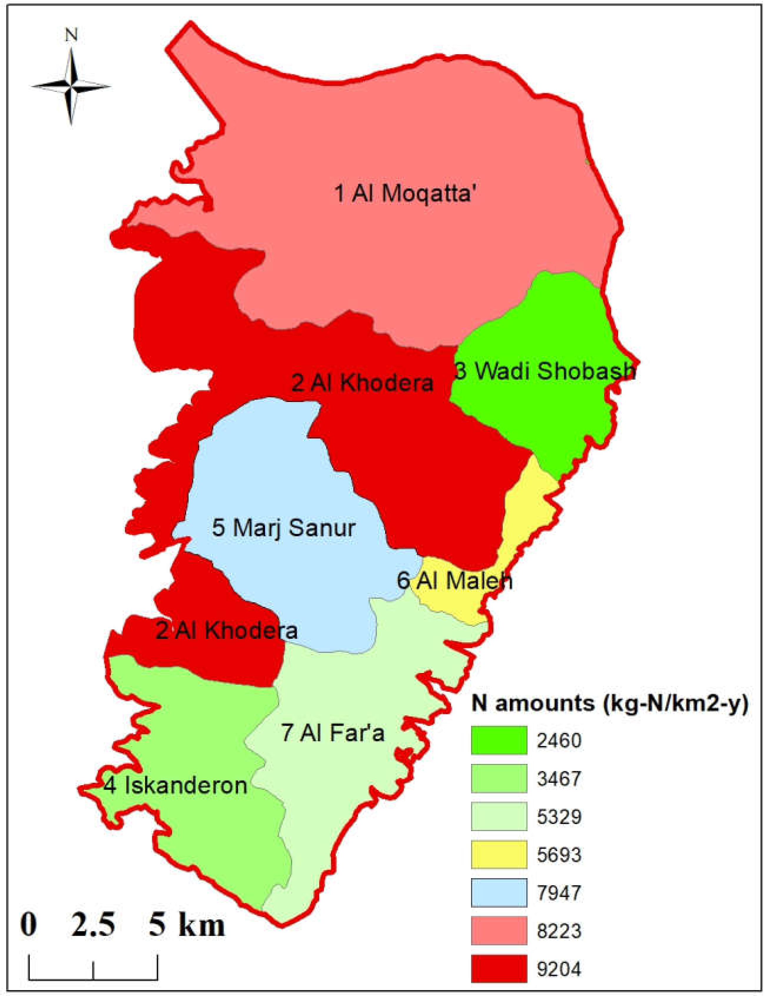
The aquifer area intersects seven watersheds and these are Al Moqatta’ (32%), Al Khodera (24%), Wadi Shobash (8%), Iskanderon (10%), Marj Sanur (11%), Al Maleh (3%), and El Far’a (12%). Three of these watersheds drain to the east toward Jordan River (Wadi Shobash, Al Maleh and El Far’a) and another three watersheds drain to the west toward the Mediterranean (Al Moqatta’, Al Khodera, and Iskanderon). Marj Sanur watershed is considered as a depression that does not have a water outflow.
The total agricultural area is 175 km2. Generally, the study area includes about 60 km2 of irrigated areas among which 3.2 km2 are greenhouses. Table 1 summarizes the land use classes for the study area. Except for olive trees, there are no rain-fed agricultural areas. There is a total of 129 wells that tap the Eocene aquifer; 45 of them are agricultural with a total annual pumping rate of 2.84 million cubic meters (MCM), five domestic wells with a total annual pumping rate of 0.97 MCM, four agricultural-domestic wells with a total annual pumping rate of 0.43 MCM and the other wells are dry or abandoned. It is worth mentioning that in Table 1 the “irrigable” areas indicate the areas that are capable of being irrigated while the areas that are actually being irrigated are denoted as “irrigated”.
2.2. Water Quantity and Quality Problems in the Eocene Aquifer
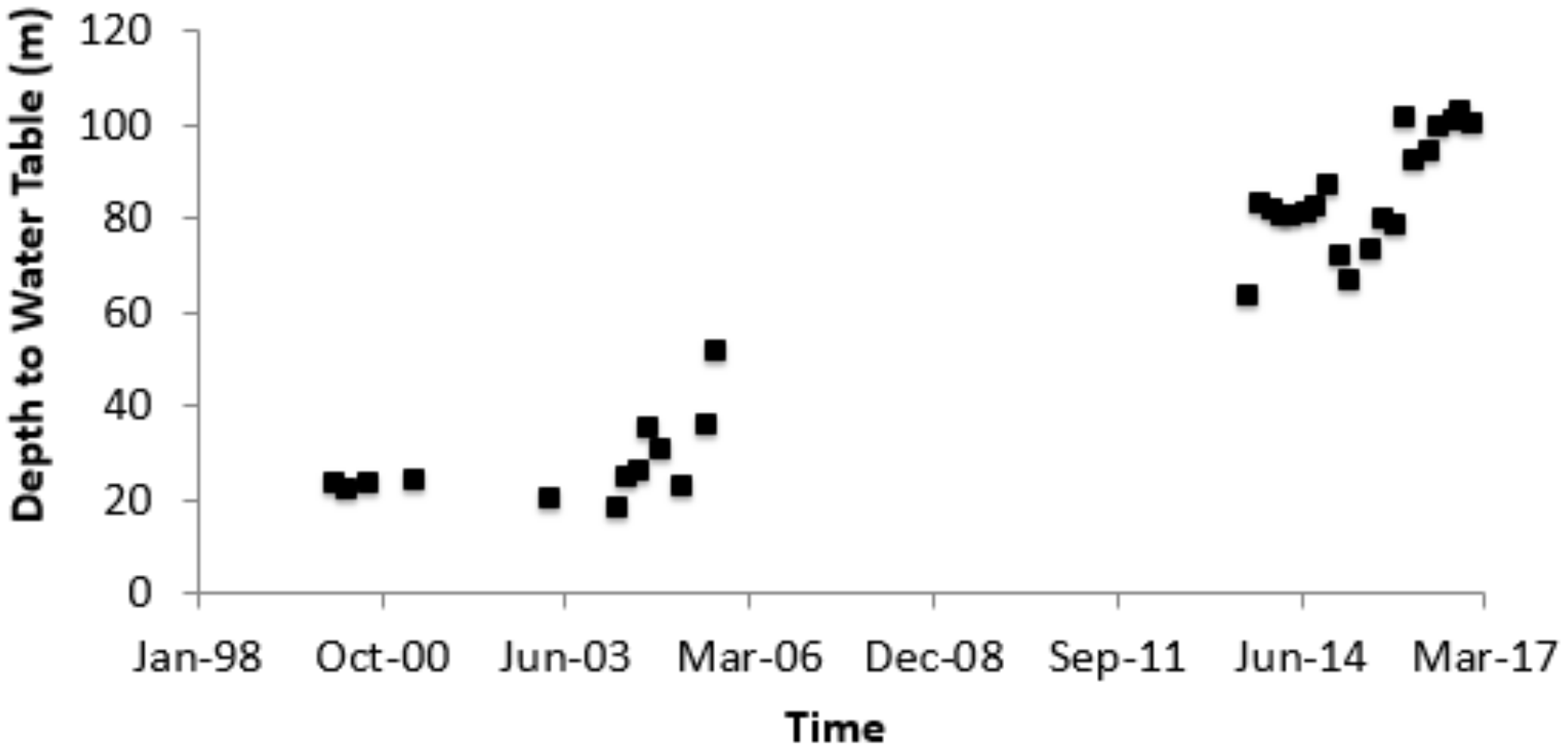
As mentioned earlier, water quantity and quality problems are taking place in the Eocene aquifer. The heavy exploitation of the aquifer due to the increasing water supply in many locations has led to the decline of the water storage in the aquifer. This is evidenced in the temporal increase in the depth to water table in many wells of the aquifer (see as an example Figure 2). This figure (Figure 2) depicts the variation of the depth to water table for a specific well that taps the Eocene aquifer. As can be inferred from the figure the average depth to water table jumped from an average value of 27 m in the period from 2000 to 2006 to the average value of 85 in the period between 2014 and 2017. The declining water storage in the aquifer has led to the abandonment of many wells (dryness) especially during the summertime where recharge is at minimum and water demand is high. The increasing water demand is driven by the increase in population and the intense agriculture. Competitive pumping from the aquifer therefore is a problem that requires management interventions.
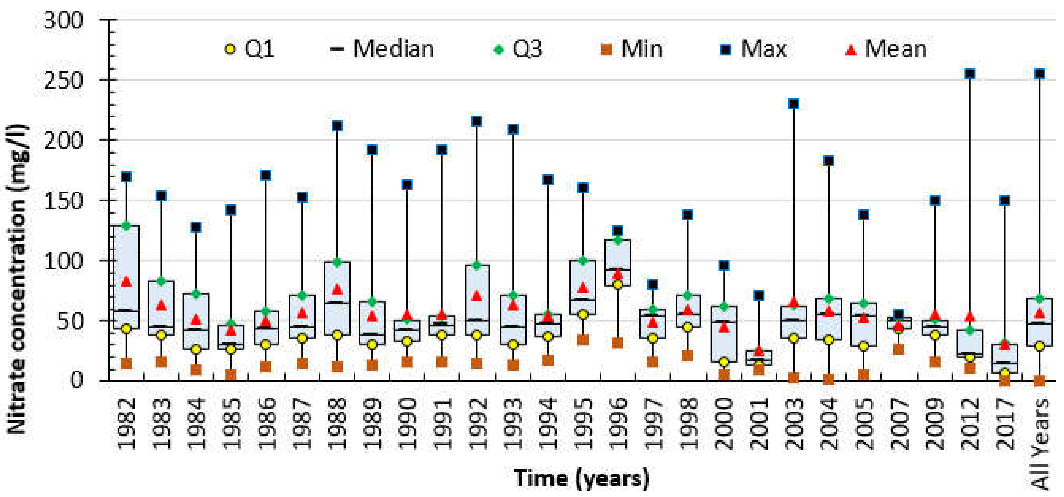
The study area is characterized by heavy agriculture that encounters an extensive use of agrochemicals [43]. In order to broadly asses the nitrate pollution problem in the aquifer, the database of the Palestinian Water Authority (PWA) was analyzed for nitrate concentrations in the Eocene aquifer. The PWA database covers the years from 1982 to 2017 with many years of unavailable data. The number of nitrate readings differ from year to year with a minimum and maximum number of readings of 4 and 38 per year, respectively with a total of 456. Figure 3 depicts the statistics of the annual nitrate concentrations in the Eocene aquifer for specific years in the period from 1982 to 2017. As can be inferred from Figure 3, the maximum nitrate concentration in the Eocene aquifer exceeds in all the years the maximum contaminant level (MCL) of 10 mg/L as N. This MCL is set by the US Environmental Protection Agency (this is equivalent to ~50 mg/L NO3). The annual mean nitrate concentrations exceed the MCL in all the years with the exception of years 1985, 1997, 2000, 2001, and 2017. The third quartile, Q3, (the 75th percentile) in all the years exceeds the MCL. When considering the 465 total available nitrate readings at once, the mean nitrate concentration exceeds the MCL while the maximum concentration is 256 mg/L. In general, the elevated nitrate concentrations indicate the presence of anthropogenic sources responsible for pollution [47].
2.3. Methodology
The methodology of the research is comprised from different components (see Figure 4). It starts by identifying all the potential sources of nitrogen in the study area. This identification implies the determination of the spatial locations of the sources based on the nature of each source (for instance point or non-point) and the type of each source (for instance fertilizers).
All the data related to each identified source were collected. To account for the spatiality of the nitrogen sources, the land use map was utilized. This enabled the allotment of the sources spatially according to the land use. GIS was used in the development of the maps that show the presence of each source along with the computation of the corresponding amount of generated nitrogen.
All possible sources of nitrogen in the study area were identified. Relevant data was obtained from many sources and through different means including pertinent reports, past studies from the literature, field visits, ground truthing, researchers at universities, official authorities, ministries, municipalities, local councils, and non-governmental organizations working in the field.
For each identified source of nitrogen, a GIS layer (shapefile) was developed to account for the spatial distribution (presence) of this source. The amount of nitrogen from each source was then estimated and the procedure for that was given in detail (Section 2.4). The assumptions were clearly stated and the data employed in the calculations were listed. Correspondingly, for the estimated amount of each nitrogen source the percentages of nitrogen species were assigned. For each nitrogen species (nitrate, ammonium, and organic nitrogen) of each source (when applicable), a GIS shapefile was created. Therefore, a set of GIS shapefiles were produced corresponding to the number of sources per each species. All the GIS shapefiles were converted to rasters to facilitate the mathematical processing. For each of the three species, the rasters were summed up. Thus, three composite rasters that represent the spatial distribution of the annual nitrogen loading for the study area were created. Each one of them represents one nitrogen species (nitrate, ammonium and organic nitrogen). A fourth raster was prepared for the total annual nitrogen. Thereafter, GIS rasters of the temporal (monthly) amounts of nitrogen were developed in order to account for the time aspect of the pollution sources based on the application (loading) time. Finally, the analysis of the developed maps was furnished with the consideration of groundwater flow characteristics.
2.4. Potential Sources of Nitrogen in the Eocene Aquifer
The potential sources of nitrogen in the area of the Eocene aquifer are as follows; infiltrating cesspits, leakage from urban sewage collection lines, dry deposition, wet deposition, treated and raw wastewater inflows to wadis, legumes, fertilizers (chemical and manure) and irrigation with polluted groundwater. All these sources are considered as non-point sources except the infiltrating cesspits and leakage from urban sewage collection lines which are in reality point sources. However, the infiltration from cesspits and the leakage from sewage lines are in general not known perfectly.
Each source was taken individually where the representative land use classes were associated with the relevant sources. Thereafter the corresponding map of each individual source was developed. The summation of all the individual maps per each species yields the spatial distribution of the annual total nitrogen amount in the study area. The following subsections summarize the implementation steps of the methodology.
2.4.1. Infiltrating Cesspits
Since the majority of the communities in the study area are not served by wastewater collection networks, the cesspits (an underground pit for the disposal of wastewater) are widely used in the study area for the disposal of wastewater [1]. In general, the cesspits are not internally coated and thus allow the downward infiltration and leakage of nitrogen. The annual nitrogen amount resulting from these cesspits was estimated using the following formula:
where: Ncesspit is the annual nitrogen amount from cesspits (kg), Pop is the population of the study area, D is the annual per capita domestic water consumption (liters), W is the wastewater generation percentage from consumed water (%), P is the percentage of the population that uses the infiltrating cesspits (%) and Cic is the concentration of the different N species in the infiltrating cesspits’ wastewater (mg/L). Ncesspit is computed three times since Cic has three different values corresponding to the three nitrogen species.
For the study area: D = 30,660 liters [48], W = 80% [1], Cic for NH4-N, NO3-N and organic-N are 151.4 mg/L, 0.4 mg/L, and 63.8 mg/L, respectively [49]. For each community, its population (Pop) was obtained [42] and the percentage of the population that uses cesspits (P) was determined (Palestinian Central Bureau of Statistics (PCBS), 2018, personal communication) and both were used in the computations.
2.4.2. Leakage from Urban Sewage Lines
Sewage systems are more recommended for the collection, transport and disposal of wastewater as compared to the cesspits [1]. However, leaky sewage lines can be considered as a potential source of nitrogen [31]. The annual nitrogen amount resulting from the leaky sewage lines was estimated using the following formula:
where: Nsewer is the annual nitrogen amount from sewage lines (kg), Pop is the population, D is domestic water consumption (L/c·year), P1 is the percentage of population connected to sewage collection networks (%), P2 is the percentage of leakage from these networks (%) and Csl is the concentrations of the different nitrogen species in the sewage lines (mg/L). Nsewer is computed three times since Cil has three different values corresponding to the three nitrogen species
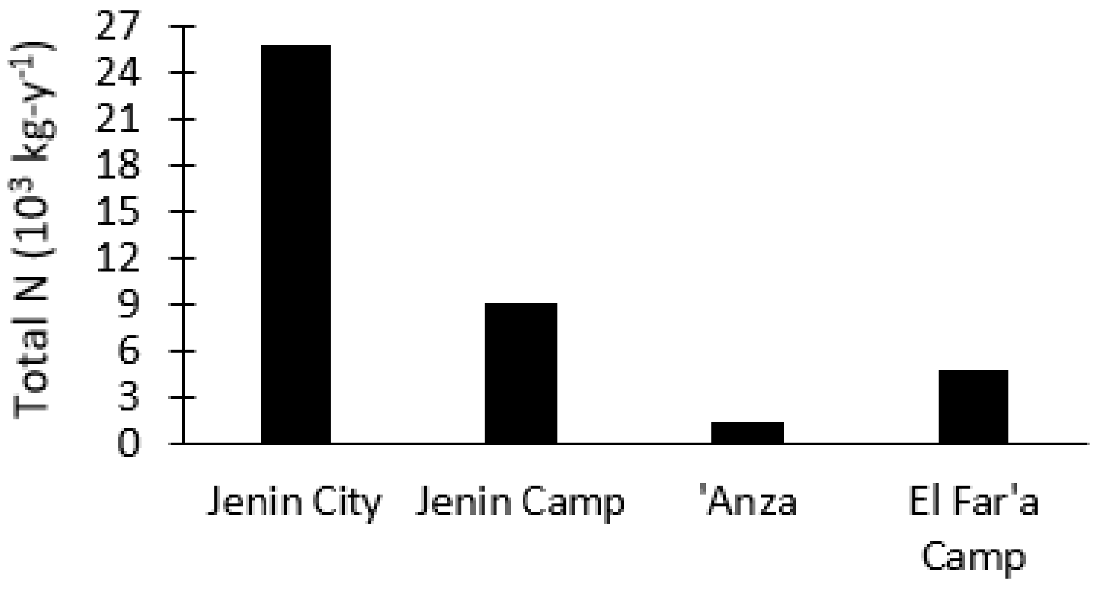
For the study area: Csl for NH4-N, NO3-N and organic-N are 67.2 mg/L, 7.7 mg/L, and 71.8 mg/L, respectively (Laboratory analysis of the sewage influent as obtained from the wastewater treatment plant of Jenin City). There are four communities in the study area that have wastewater collection networks and these are Jenin City, Jenin Camp, ‘Anza Village and El Far’a Camp. The corresponding percentages of the population serviced by sewage networks (P1) are 74%, 98%, 81%, and 88%, respectively. The percentage of leakage from these networks (P2) varies in reality yet it was assumed to equal 20% based on personal communications as no data was available in this regard.
2.4.3. Dry Deposition
Dry deposition is the falling of pollutants including gases and particulate matter from the atmosphere to the ground surface [50]. The annual nitrogen amount resulting from this deposition was estimated using the following formula:
where: Nddep is the annual nitrogen amount from dry deposition (kg), DDR is the annual dry deposition rates for NH4-N and NO3-N (kg/km2) and A is the total area (km2). For the study area the annual dry deposition rates (DDR) for NO3-N and NH4-N were taken as 490 and 95 kg/km2, respectively [51]. Nddep is computed two times since DDR has two different values corresponding to the two nitrogen species; NO3 and NH4.
2.4.4. Wet Deposition
Wet deposition is the transfer of pollutants from the atmosphere to the earth by inclusion or solution in precipitation [50]. The annual nitrogen amount due to wet deposition was calculated as follows:
where: Nwdep is the annual nitrogen amount from wet deposition (kg), WDR is the wet deposition concentrations for the different nitrogen species (mg/L) and R is the annual rainfall volume (m3). For the study area the annual wet deposition concentrations for the different nitrogen species were taken as 0.79 and 0.58 mg/L for NO3-N and NH4-N, respectively [52]. Nwdep is computed two times since WDR has two different values corresponding to the two nitrogen species; NO3 and NH4.
The long term average monthly rainfall for the last 10 years in the study area was calculated based on the data available from the distributed rainfall gauges (Palestinian Meteorological Department: Personal Communication, 2018). As a result, wet deposition was temporally distributed according to this rainfall. GIS was used to develop the Thiessen polygons of the spatial distribution of the rainfall based on the locations of the gauges. Wet deposition was spatially distributed throughout the study area based on these polygons.
2.4.5. Legumes
Legumes have root nodule bacteria that can fix nitrogen for the plant from free nitrogen gas in the atmosphere [53]. The annual nitrogen amount from the legumes was calculated using the following formula:
where: Nlegumes is the annual nitrogen amount from legumes (kg), L is the annual contribution rate of nitrogen from legumes (kg/km2) and A is the area planted by legumes (km2). Beans, String beans, Peas, Chickpeas, Lentils and Alfalfa are leguminous plants that are common in the study area. For the study area, the annual contribution rate of 560 kg/km2 of NO3-N from legumes was considered based on the work of Cox and Kahle [47]. The area planted by legumes in the study area is about 32 km2.
2.4.6. Fertilizers (Chemical and Manure)
In the study area, fertilization is taking place by the use of chemical fertilizers and manure. Chemical fertilizers are a vital input for increasing the plants’ productivity. Plenty of studies from the literature highlight the contribution of fertilizers (chemical and manure) to the nitrate pollution of groundwater [11,12,16,23,24,25,41]. The annual nitrogen amount resulting from chemical fertilizers is estimated using the following formula:
where: Nfer is the annual amount of nitrogen source from chemical fertilizers (kg), A is the fertilized area (km2), F is the annual fertilization rate of the different types of fertilizers (kg/km2), PN1 is the percentage of nitrogen in the fertilizer and PN2 is the percentages of the nitrogen species in each fertilizers type (%). Chemical fertilizers are extensively used in the study area over four land use classes (irrigated crops, irrigated trees, green houses and rain-fed areas). Nfer is computed two times corresponding to the two nitrogen species; NO3 and NH4.
The most common fertilizers used in the study area are Ammonium Sulfate, Urea and Ammonium Nitrate as summarized in Table 2.
Manure is widely used in the study area for enhancing plants’ productivity. All the waste and manure from cows, veals, calves, sheep, goats, and poultry that exist in the study area are used for fertilization. The number of animals of each type, the corresponding annual production of waste and the mass concentration of the different nitrogen species in the waste were obtained [54,55]. As a result, the annual nitrogen amount from manure application was calculated as follows:
where: Nmanure is the annual nitrogen amount from manure (kg), n is the number of animals of each type (head), K is the daily production of waste per head of each animal type (kg/head) and M is the mass concentration of the different nitrogen species in animals’ waste (g/kg). The K values for the different animal types are 55.5, 5.6, 5.6, 1.1, 2.6, and 0.1 for cows, veals, calves, sheep, poultry, and goats, respectively. The mass concentrations of the different nitrogen species in animals’ waste (g/kg) are summarized in Table 3. The annual nitrogen amount due to manure application was spatially distributed among four land use classes in a uniform manner (irrigated crops, irrigated trees, green houses and rain-fed areas).
2.4.7. Discharged Raw and Treated Wastewater to Wadis
Wadis receive treated wastewater from the effluent of wastewater treatment plants (WWTPs) located within the study area. In addition, wadis also receive raw (untreated) wastewater from three sources: evacuation of coated cesspits, sewage lines not connected to WWTPs and from the sewage lines that are connected to WWTPs but when the WWTPs are at full capacity. The volumes of treated and raw wastewater inflows to wadis and the associated nitrogen concentrations were considered in the calculations. The annual nitrogen amounts from these sources were calculated as follows:
where: Nwadis is the annual nitrogen amount from wadis (kg), N1 is the annual nitrogen amount from the effluent of Jenin City and ‘Anza Village WWTPs (kg), N2 is the annual nitrogen amount from the evacuation of coated cesspits (kg), N3 is the annual nitrogen amount from the sewage lines not connected to WWTPs (kg), N4 is the annual nitrogen amount from the sewage networks connected to WWTPs but when the WWTPs are at full capacity, E1 is the effluent of Jenin WWTP (m3), E2 is the effluent of ‘Anza WWTP (m3), U is the concentration of the different nitrogen species in the WWTPs effluent (Jenin and Anza WWTPs: Personal Communication, 2018) (mg/L), Pop is the population [42], D is the domestic water consumption (L/c·year) [48], W is the wastewater generation factor [1], P is the percentage of population that use the coated cesspits (%), C is the concentration of the different nitrogen species in the wastewater of the coated cesspits (mg/L) [49], P1 is the percentage of the population connected to sewage networks that are not connected to WWTPs (%), P2 is the percentage of leakage in these networks (%), L is the concentration of the different nitrogen species in the sewage networks (mg/L), J1 is the percentage of the population connected to sewage networks that are connected to WWTPs yet this sewage is not received by the WWTPs due to their full capacity (%) and J2 is the percentage of leakage in these networks (%). The nitrogen concentrations in the treated wastewater are 10, 30, and 15 mg/L for NH4-N, NO3-N and organic nitrogen, respectively (Palestinian Water Authority, personal communication, 2018).
2.4.8. Irrigation
Another potential source of nitrogen in the study area is the irrigating water that is contaminated by nitrogen. Many studies in the literature highlighted this as a potential source of nitrate pollution in groundwater [23,24]. Two sources of irrigation water are available in the study area; groundwater and treated wastewater. The greenhouses are irrigated only by groundwater from the Eocene aquifer while open fields are irrigated from groundwater and treated wastewater. The annual nitrogen amount from irrigation is calculated as follows:
where: Nirr is the annual nitrogen amount due to irrigation (kg), AO1 is the area of the fields that are irrigated by groundwater (m2), IRO is the irrigation rate for the open fields (m3/m2), C1 is the concentration of the different nitrogen species in the groundwater that is utilized for irrigation (mg/L), AO2 is the area of the open fields that are irrigated by treated wastewater (m2), C2 is the concentration of the different nitrogen species in the treated wastewater that is used in irrigating the fields (mg/L), AG is the area of the greenhouses (m2) and IRG is the irrigation rate for greenhouses (m3/m2).
The corresponding nitrogen amounts were spatially distributed over open fields and areas of greenhouses in a uniform manner. In the study area, the annual irrigation rates for open fields and greenhouses are 0.55 and 0.9 m3/m2, respectively based on personal communication. Average concentrations of ammonium, nitrate and organic-N in groundwater are 0.3, 12.3, and 2.2 mg/L respectively (lab analysis based on the average of winter and summer tests for five agricultural wells) while for the treated wastewater they are 10, 30, and 15, respectively (based on personal communication).
3. Results and Discussion
This section presents the annual, temporal and spatial on-ground nitrogen loadings (nitrogen amounts) in the area of the Eocene aquifer and the corresponding monthly nitrate leaching. It also illustrates the relationship between the on-ground nitrogen loading (practices) and the nitrate concentrations in two selected wells located in the Eocene aquifer.
3.1. Annual Nitrogen Amounts from the Different Sources
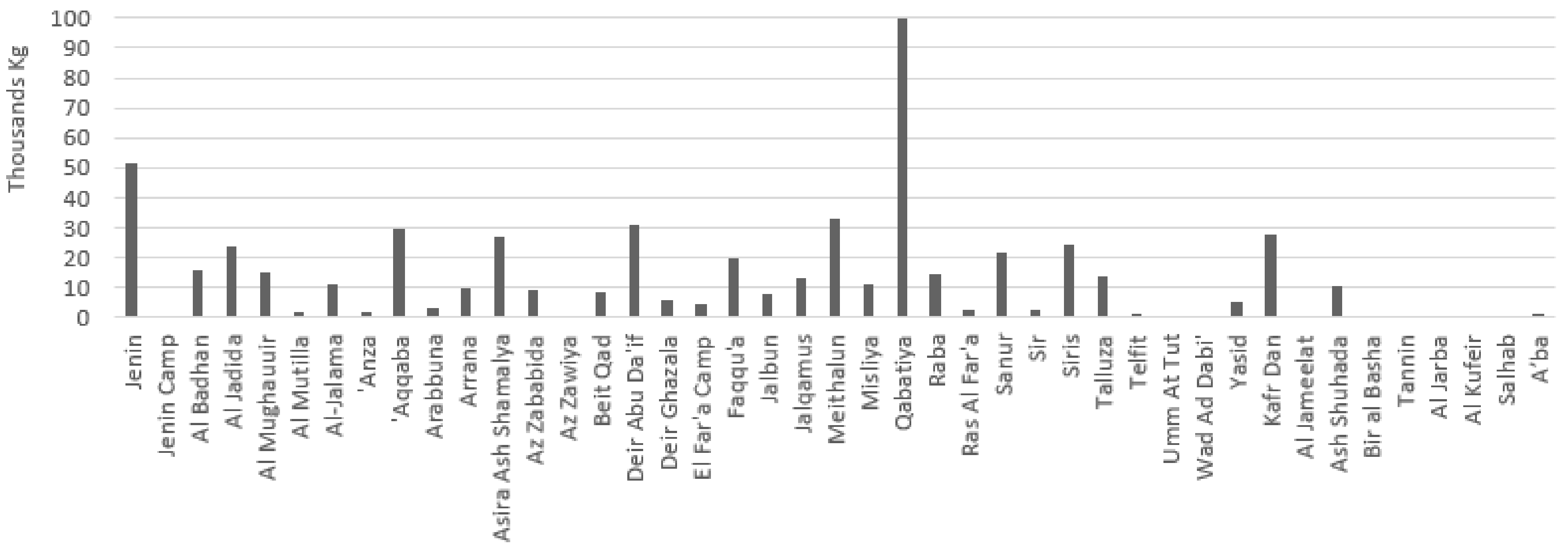
In this section, the amounts of nitrogen from each source are provided. Figure 5 depicts the annual nitrogen amounts from the infiltrating cesspits for the communities of the study area. High nitrogen amounts are associated with high population and vice versa.
Regarding the spatial distribution of the nitrogen from cesspits, it is assumed that the loading from all the infiltrating cesspits in a certain community is uniformly distributed over the area bordered by the community. It should be kept in mind that this loading was distributed spatially over community border (called sometimes as the physical plan) and was therefore treated as a non-point source though it is in reality a point source. The total annual nitrogen amount due to this source is 581,593 kg. The temporal distribution of loading from infiltrating cesspits goes in line with the temporal variations in the average per capita monthly water consumption rate. The average per capita daily consumption rate is 73 liters in winter, 84 liters in spring and autumn and 95 liters in summer.
Figure 6 depicts the total annual nitrogen amounts due to the leakage from the sewage lines for the served communities where this amount is 41,076 kg. The nitrogen amounts resulting from these systems is temporally and spatially distributed following the same approach used for infiltrating cesspits.
The annual nitrogen amount due to dry deposition for the entire study area is 268,317 kg. Since the available data are limited, the annual nitrogen loading is spatially distributed among the study area in a uniform manner. The total amount of annual nitrogen in the study area due to wet deposition is 282,356 kg.
The annual amount of nitrogen from legumes in the study area is 17,920 kg. Legumes in the study area are planted and harvested between September and May. As such, the nitrogen amount from legumes was uniformly distributed in these nine months. The nitrogen loading from this source was uniformly distributed over the areas that represent the areas planted by crops using the GIS shapefile of the land use.
As for chemical fertilizers, the annual amounts of NH4-N (kg) from Ammonium Sulfate, Urea and Ammonium Nitrate are 900,770; 11,440 and 147,146; respectively with a total of 1,059,357 kg. The total amount of NO3-N is 147,146 kg for the entire study area. Since the annual nitrogen amount due to chemical fertilization of each land use class was determined, the loading was spatially distributed among these classes. The fertilization time or period for each agricultural land use class that is subject to fertilization was identified. Accordingly, this amount was temporally distributed. The total annual nitrogen amount due to manure application for the study area is 36,395 kg. Farmers prefer to apply the manure in the months of September, October, and November (prior to rainfall). The annual nitrogen amount from manure application was uniformly distributed over these three months to arrive at the temporal distribution.
The total annual nitrogen amounts discharged to wadis are 243,002, 8368, and 47,582 kg, respectively. These wadis are Al-Moqata, Masin, and El Far’a. So, the total loading was spatially distributed over the outlines of the three wadis using GIS. The allocation was determined based on how much treated and raw wastewater are discharged (by the communities) to each wadi. The temporal distribution of loading from these sources goes in line with the monthly variations in the per capita water consumption.
The annual loadings from NH4-N, NO3-N, and organic-N due to irrigation are 15,038, 428,471, and 81,407 kg, respectively. The nitrogen amounts from this source were temporally distributed given that open fields are not irrigated in the rainy months and that greenhouses are irrigated for the whole year. A summary of the annual nitrogen amounts from the different sources in the Eocene aquifer area is provided in Table 4.
As indicated by Table 4, the total annual amount of nitrogen in the study area is approximately 3260 tons with an average amount of 7028 kg/km2. It can be clearly seen that fertilizers (chemical and manure) are the main source of on-ground nitrogen loading with about 1243 tons (38% from the total) especially when adding to that an additional 16% that represents the nitrogen that comes from the irrigation with contaminated water. It is noticed that the sources related to wastewater discharge (infiltrating cesspits, leakage from urban sewer lines and treated and raw wastewater inflows to wadis) contribute together approximately 922 tons (28% from the total). Legumes contribute the least amount of nitrogen (0.55% from the total). Further analysis shows that NH4-N is the dominant form of nitrogen with a contribution of 58%. This is because NH4-N is the main nitrogen form in the composition of the fertilizers in the study area. NH4-N is followed by NO3-N and organic-N with approximately 31% and 11% from the total nitrogen, respectively.
3.2. The Spatial Distribution of the Total Nitrogen
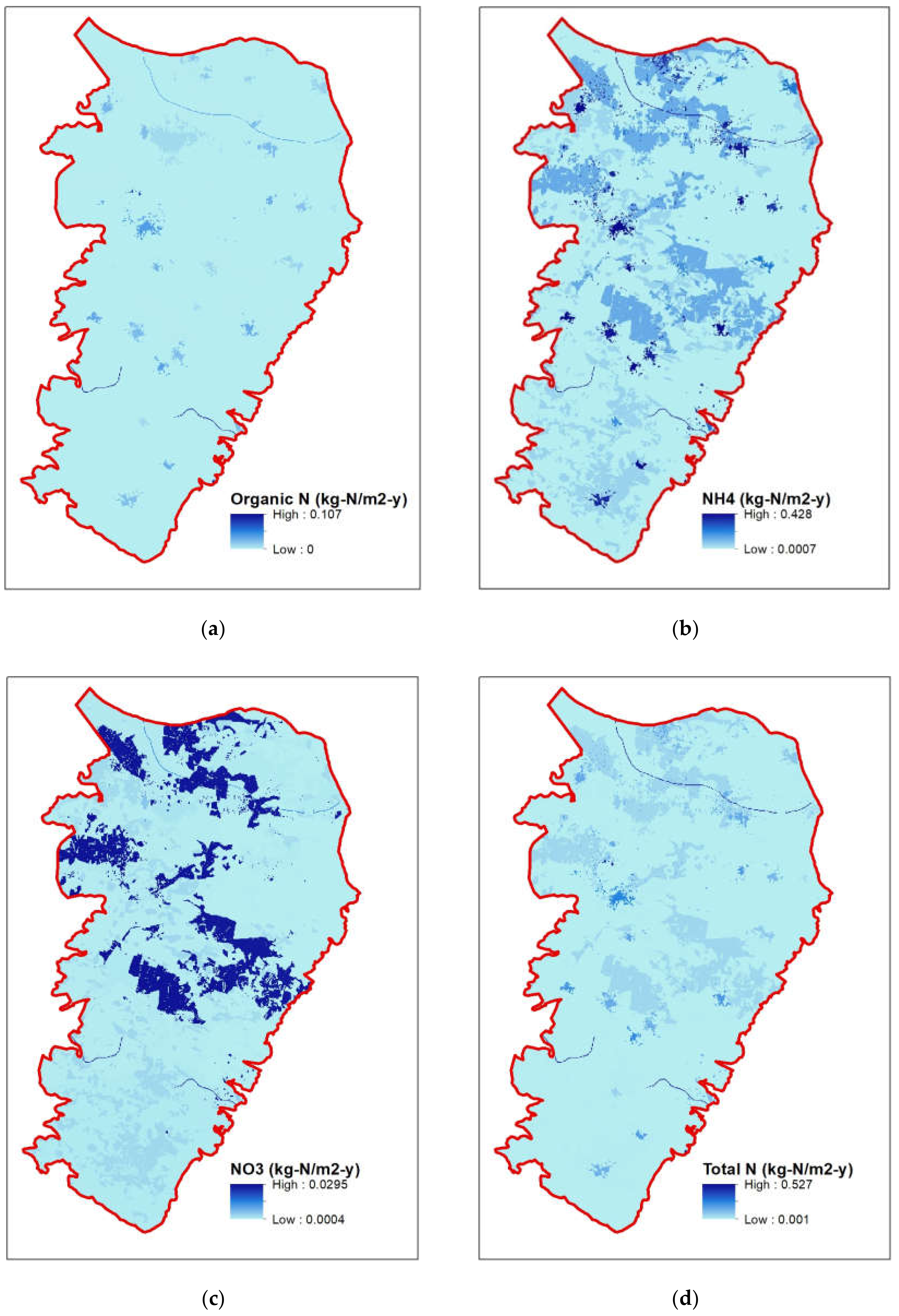
Nitrogen sources and corresponding amounts differ from one place to another considering the different activities and their respective locations. This is apparent based on the land use map for the study area. Figure 7 shows the spatial distribution of the annual organic nitrogen (Figure 7a), ammonium (Figure 7b), nitrate (Figure 7c) and total on-ground nitrogen loading (Figure 7d) in the study area in the units of kg-N/m2.
It is found that the total annual rates of nitrogen range from about 0.001 to about 0.527 kg-N/m2 with an average annual rate of 0.007 kg-N/m2 or 7028 kg-N/km2. This average rate is approximately 60% of the rate in the Sumas-Blaine aquifer of Washington State, USA which is an area that is characterized by heavy agricultural practices [24]. On the other hand, this rate of 7028 kg-N/km2 exceeds that for the Ebro River Basin, Spain which is 5118 kg-N/km2 [23]. As for the individual nitrogen species, the minimum and maximum rates are approximately 0.0007 to 0.428 for NH4-N, 0.0004 to 0.0294 for NO3-N and 0 to 0.107 for organic-N all in kg/m2·y.
When examining the map of the on-ground total nitrogen (Figure 7d), it is noticed that this map is highly dependent on the spatial distribution of the agricultural areas that were characterized based on the land use map. Most of the areas that have elevated nitrogen amounts are agricultural areas. This is due to the extensive use of fertilizers (chemical and manure) and irrigation with water of elevated nitrogen concentration. It is also worth mentioning that the southern parts of the study area do not encounter, in general, elevated nitrogen amounts due to the inexistence of heavy agricultural activities.
The spatial distribution of the nitrogen amount was analyzed for the different soil types present in the study area. The total annual nitrogen amounts (tons) for Terra Rossa, Mediterranean Brown Forest Soils, Alluvial Soils, Colluvial-Alluvial Soils, and Brown Alluvial Soils (Vertisols) are 1021; 332; 1050; 512 and 343; respectively. The corresponding values in the units of kg/km2 are 4738; 4549; 13,131; 8,667 and 11,185; respectively.
3.3. The Temporal Distribution of the Total Nitrogen Amounts
This part aims to estimate and discuss the monthly variations of the on-ground nitrogen amounts generated in the study area. The estimation of the temporal variation in the nitrogen amounts is essential since the temporal nitrate leaching to the aquifer relies chiefly on this. In addition, knowing when nitrogen amounts are being introduced to the surface would facilitate the development of management plans especially when the time aspect is to be taken into consideration. Table 5 summarizes the monthly total amounts of nitrogen in the area of the Eocene aquifer. It can be clearly seen that the highest amounts occur in autumn and winter seasons (September through February) with approximately 2140 tons (66% of the total annual nitrogen amount from the different sources). This can be attributed to the extensive fertilization and wet deposition phenomenon by that time.
On the other hand, the loading in the spring and summer seasons (March through August) together is about 1119 tons which forms 34% of the total annual nitrogen amount from the different sources. It is worth mentioning that ModelBuilder of ArcMap was used to compute the total monthly on-ground nitrogen loadings.
3.4. Nitrate Leaching to Groundwater
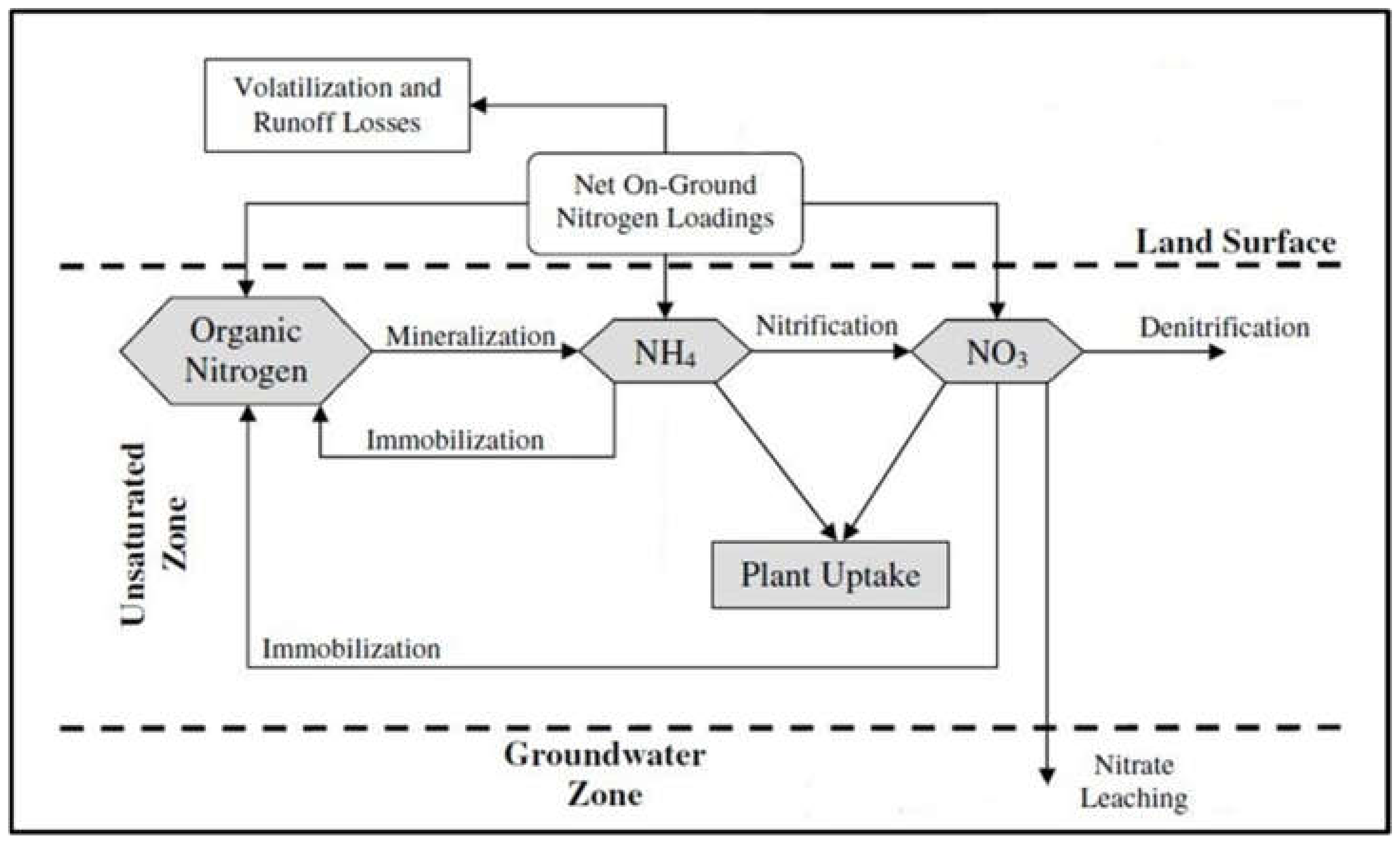
To enrich the work, the nitrate leaching to the Eocene aquifer from the unsaturated zone was spatially quantified. The importance of the evaluation of the temporal distribution of the nitrate leaching comes from the fact that the development of a nitrate fate and transport model for the Eocene aquifer necessitates this. Figure 9 shows the overall schematic that describes the integrated approach to predict nitrate leaching to groundwater.
As can be inferred from Figure 9 and based on the common understanding, nitrate leaching to the aquifer depends on the on-ground nitrogen loading, surface losses, soil kinetics, soil drainage capacity, and recharge. The critical part of this approach is the simulation of the kinetics of the unsaturated zone. This simulation can be accomplished using specialized soil models. Since the quantification of the nitrate leaching to the Eocene aquifer is beyond the scope of this manuscript, percentages from the on-ground nitrogen loading were utilized instead of soil modeling. These percentages were obtained based on the literature. We do realize the high uncertainty associated with these percentages, especially when considering that these percentages are for different sites. These estimates of nitrate leaching are merely to provide a complete picture and to enhance the analysis. In addition, these estimates can be considered as the starting point for any future modeling effort for the fate and transport of nitrate in the Eocene aquifer.
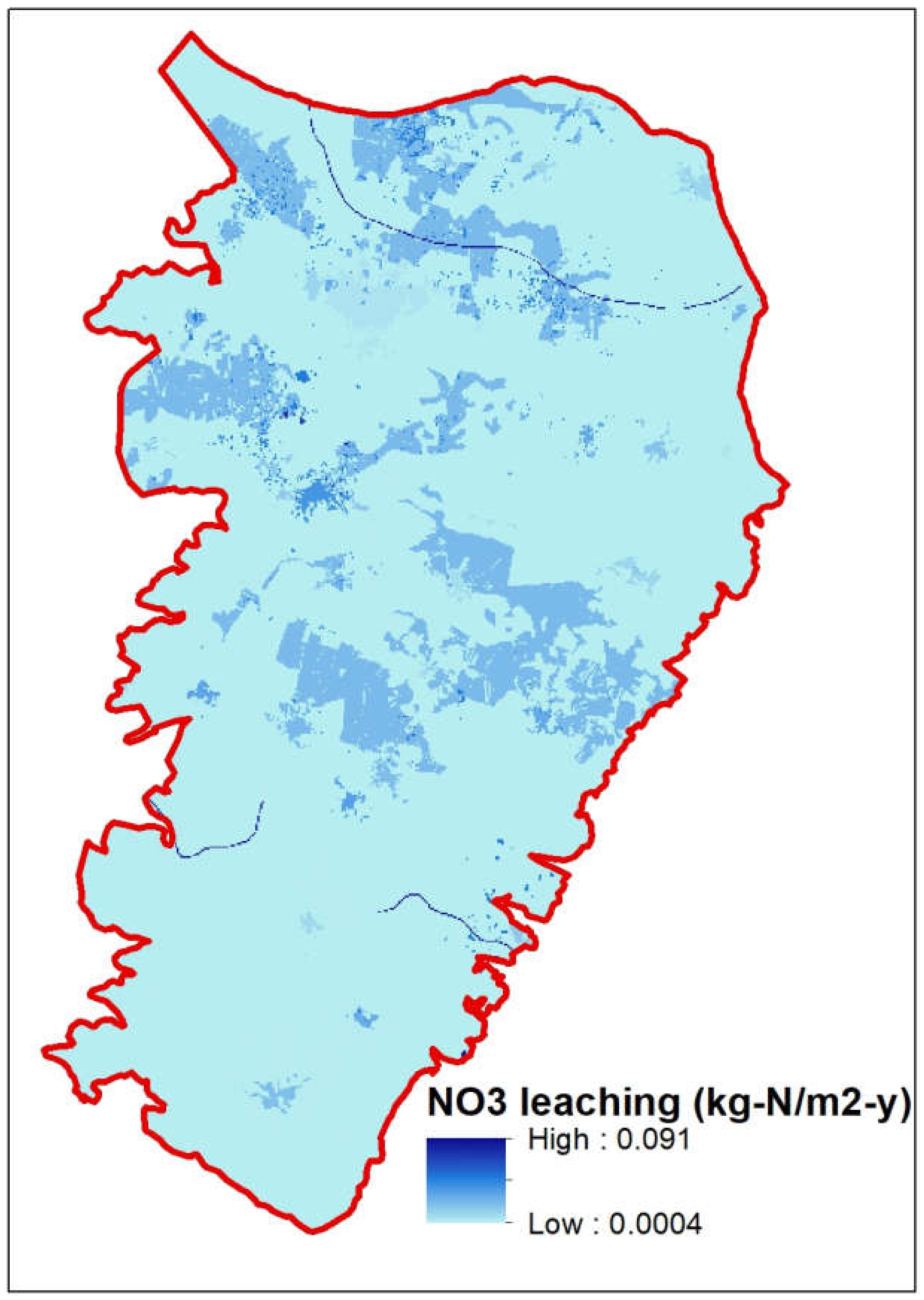
To address the ground surface losses, generally, 44% of the on-ground NH4 loading will be lost due to volatilization [56]. Moreover, 29% of the on-ground NH4, NO3 and organic-N loadings are subject to runoff losses [57]. The main soil kinetic transformations of nitrogen species are: mineralization of organic-N to NH4 where 18% of the available organic-N will be mineralized to NH4 [58], immobilization of NH4 to organic-N where 27% of the available NH4 will be immobilized to organic-N [59], nitrification of NH4 to NO3 where 64% of the available NH4 will be nitrified to NO3 [60], plant uptake of NH4 and NO3 where 9% of the available NH4 and 8% of the available NO3 will be taken up by plants [61], immobilization of NO3 to organic-N where 10% of the available NO3 will be immobilized to organic-N [59] and finally denitrification of NO3 where 15% of the available NO3 will be nitrified [59]. After considering the surface losses and the soil kinetics, 67% of the remaining NO3 in the unsaturated zone is subject to leaching to the aquifer [62]. Eventually, the NO3 leaching to groundwater is estimated and spatially distributed (see Figure 10). It is found that the annual leaching rates of nitrate range from about 0.0004 to about 0.091 kg-N/m2 with an approximate average annual rate of 0.002 kg-N/m2 or 1,968 kg-N/km2. To address the temporal variation of nitrate leaching to the Eocene aquifer, Table 6 was prepared. The highest potential of nitrate leaching to the Eocene aquifer is during October. It should be kept in mind that the temporal amounts of nitrate leaching are potential amounts and the time of arrival to the aquifer from the ground surface varies spatially throughout the study area. The increase in the depth to the water table (as evidenced in Figure 2) will increase the travel time through the unsaturated zone and thus there will be a noticeable lag between surface application of nitrogen and the arrival to the water table of the aquifer as nitrate.
3.5. Nitrogen Loading Amounts and Nitrate Concentration in Groundwater
In general, the severity of nitrate occurrence in groundwater is indicated by the high concentrations in the wells tapping the aquifer. Such elevated concentrations would transpire from the existence of many sources of nitrogen in the proximity of the sampled wells and/or the presence of the well at a downstream location to an upstream area of high potential nitrogen amounts. The latter depends on the groundwater flow direction and relies as well on how long the sources have been in place because of the lag time between the location of the on-ground nitrogen application and the travel time from the surface to the water table and the travel time to the well location.
The groundwater flow direction within the aquifer is from the south to the north in general while in the middle it is to the east and to the northeast. Accordingly, it was found that the most contaminated wells by nitrate are found in the north and in the east where heavy agricultural practices do exist.
To further highlight the impact of groundwater flow direction and land use practices on the nitrate concentration (and distribution) in the Eocene aquifer, particle path lines for selected wells were developed and analyzed (see Figure 11). As can be noticed, Figure 11 depicts in the background the agricultural areas in order to better associate the on-ground activities with the contribution area of each well. The development of the path lines was carried out using MODPATH software (A Particle-Tracking Model for MODFLOW). Two wells were considered for this analysis, Well 1 (Figure 11a) and Well 2 (Figure 11b). Well 1 is located in an area that is under heavy agricultural practices. The nitrate concentration in this well was measured in July 2019 and was found to be 48.4 mg/L. This concentration is close to the MCL of 50 mg/L. Therefore, it is apparent from Figure 11a the association between the on-ground activities and the elevated nitrate concentrations in the aquifer. The nitrogen loading associated with agricultural activities was found to be the highest in the study area (see Table 4 for the fertilization). The same logic applies to Well 2 which is located in an area that does not have noticeable agricultural activities within the capture zone of this well (see Figure 11b). The measured nitrate concentration for this well in July 2019 was 1.8 mg/L. It should be kept in mind that there are other factors that affect this relationship between the on-ground activities and the nitrate concentrations at certain receptors. These include for instance the recharge amount, nitrate leaching to groundwater from the unsaturated zone and travel time within the unsaturated zone and in the aquifer. In addition, the pumping rates of the specific wells (for instance W1 and W2) or from the nearby wells play an important role in determining the processes of the advective transport of nitrate in the aquifer and its distribution. Table 7 summarizes certain influential parameters that affect the nitrate concentration in the sampled wells.
In order to estimate the travel time in the unsaturated zone (see Table 7), we used the following equation:
where ta is the travel time through the unsaturated zone (days), ne is the effective porosity (L0), L is the thickness of the unsaturated zone (m), R is the recharge rate (m/d) and Ks is the saturated hydraulic conductivity (m/d). This equation was developed by Szestakow and Witczak, 1984 (as cited in [63]). The thickness of the unsaturated zone (L) equals the difference between the elevations of the ground surface and the water table. To determine an average value of L for the contribution area of each well, we extracted the water table grid from the simulation results of MODFLOW, converted this grid to a GIS shapefile, subtracted that from the corresponding ground surface elevation and computed a weighted average of this difference based on the feature areas. Equation (14) was used due to its simplicity. However, it must be kept in mind that this equation gives approximated values and it should be realized that only advection is considered herein without for instance the inclusion of the dispersive flow. In addition, Darcy flux is assumed to equal the recharge (R).
As for the travel time in the aquifer, MODPATH was utilized to determine the cumulative travel time of the particles across the path lines. Table 7 presents the maximum travel times (farthest particles) for selected path lines for the two wells. The variation of the travel time for the different path lines for a specific well is a function of the path line length, the hydraulic conductivity (the aquifer is heterogeneous) and the hydraulic gradient which depends largely on the distribution of the wells and the recharge. The time lag between the introduction of on-ground nitrogen loadings and the appearance in the sampled wells is evident in Table 7. The long travel time from the location of on-ground nitrogen application and the location of the well makes it more important to consider a year-to-year temporal variation rather than from month to month. However, this issue requires further analysis.
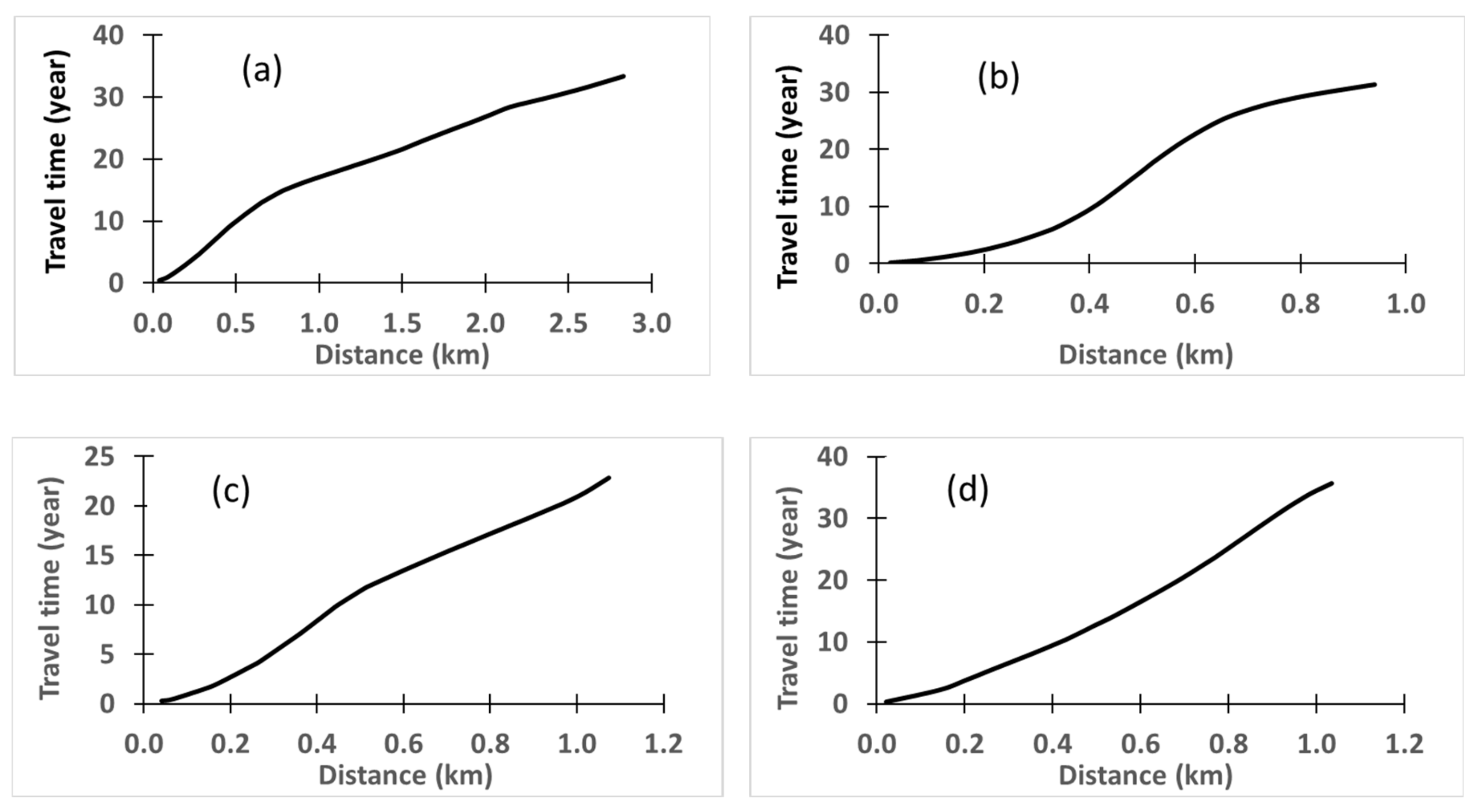
To further investigate the travel time aspect of the transport of nitrate in the Eocene aquifer, Figure 12 was developed based on the output from MODPATH and further processing by GIS. Figure 12 shows four different relationships between distance to well and particle travel time for W1 (see Figure 11). When superposing these dissimilar behaviors as in reality and when also considering the variability in the travel time through the unsaturated zone it will be difficult to relate perfectly between on-ground nitrogen rates and nitrate concentrations in groundwater. All in all, the different travel times and the different path lines will affect the nitrate fate and transport as this might lead to nitrate production (nitrification) or removal (denitrification). This can put the groundwater under conditions of presence or absence of dissolved oxygen and electron donors (carbon for instance). Therefore, it should be clear that all processes related to nitrate presence are site specific and differ from location to location within the aquifer itself. Indeed, one can resort to model the entire system (based on Figure 9) yet a huge uncertainty is embedded that must be impeccably addressed.
All of that adds to the intricacy of the nitrate occurrence in the groundwater and its distribution. It is worth mentioning that although Figure 11b shows almost the inexistence of agricultural areas within the path line area of W2 yet on-ground nitrogen loading does not equal zero since there are other minor sources that contribute like dry and wet depositions (see Table 7). Nevertheless, the on-ground nitrogen loading for W1 is almost nine times more than that of W2. It is worth to notice the difference between pumping rates and total recharge for the two wells which indicates a deficit and leads to a decline in the water table.
4. Conclusions
This paper focuses on the spatial and temporal identification of the sources of nitrogen in the area of the Eocene aquifer (Palestine). The methodology employed in this paper is straightforward, simple, easy to implement and the outcome is very informative. The cornerstone of the methodology is the use of GIS which has become a favorable and useful tool worldwide. Results indicate that the estimated total annual nitrogen amount due to the different sources in the study area is about 3260 tons. The estimated annual nitrogen amounts in the study area range from about 0.001 to about 0.527 kg/m2 with an average value of 7028 kg-N/km2. Approximately 38% of this amount is attributed to the use of fertilizers (chemical and manure). NH4-N is the dominant type of nitrogen with a contribution of about 58%. It is also found that the highest amount of nitrogen (with approximately 66% from the total annual nitrogen) was encountered in the autumn and winter seasons. The potential annual nitrate leaching to the aquifer is 1968 kg-N/km2. Since this was estimated based on many assumptions from the literature then there is a need to do a detailed modeling and monitoring to better quantify the leaching rates spatially and temporally.
It is evident from the use of the particle tracking analysis the strong link between the high on-ground nitrogen loading and the elevated nitrate concentration. This in fact highlights the importance of utilizing fate and transport models (NFTMs) for better assessment of the spread and extent of nitrate occurrence in the aquifer. In addition, NFTMs assist in developing prospective management options to remedy the contamination problem. Needless to mention that the development of the NFTMs requires the determination of the spatial distribution of nitrate leaching to groundwater. The determination of nitrate leaching relies on many factors including the amount of recharge, soil physical and chemical characteristics, plant uptake and most importantly the on-ground nitrogen loadings and corresponding surface losses. The entire system of nitrogen loading, nitrate leaching, groundwater flow and nitrate fate and transport forms a chain that encompasses stresses and responses that are necessarily to be simulated in order to better manage the contamination problem. The identification and quantification of on-ground nitrogen sources is the first and vital step in this management system.
The identification and quantification of the nitrogen sources require the availability of detailed data that cover different aspects (for instance fertilizer application rates and dry deposition) and must be treated in different ways (for instance the spatial distribution of the point and non-point sources). With this situation in mind, the issue of parameter uncertainty must be thought of. The uncertainty in this regard arises from the identification of the locations of nitrogen sources, the actual practices and application rates, the characteristics of the surface and the soil and not to mention the accuracy of the land use map. For instance, the manure generation amounts, transfer, application locations and composition were in general based on guesstimates that combine reasoning, field investigation, personal communication and literature. There is an embedded uncertainty in the determination of the on-ground nitrogen amounts and indeed the corresponding nitrate leaching to groundwater. Further work is thus needed to address this uncertainty in terms of defining an upper and lower bounds on the estimates of the key influential parameters.
Finally, although the available data are limited for the study area, the work provides an overall valuable insight about the nitrogen sources in the area of the Eocene aquifer. This will assist the decision makers to highlight the areas of high potential to pollute the Eocene aquifer and will aid in the formulation of proper strategies to protect the water quality of the aquifer. It is for the first time such a detailed quantification of nitrogen sources is carried out for the study area and certainly this will pave the road for additional related studies for the area of the Eocene aquifer and other aquifers in Palestine.
Author Contributions
Conceptualization, M.N.A. and T.G.J.; methodology, M.N.A.; software, M.N.A. and T.G.J.; validation, M.N.A., T.G.J. and S.M.S.; formal analysis, M.N.A., T.G.J. and S.M.S.; investigation, T.G.J.; resources, M.N.A.; data curation, M.N.A. and T.G.J.; writing—original draft preparation, M.N.A.; writing—review and editing, M.N.A., T.G.J. and S.M.S.; visualization, T.G.J. and S.M.S.; supervision, M.N.A.; project administration, M.N.A.; funding acquisition, M.N.A. All authors have read and agreed to the published version of the manuscript.
Funding
This research was funded by the Netherlands Representative Office, Ramallah, Palestine under the second Palestinian-Dutch Academic Cooperation on Water (PADUCO-II).
Acknowledgments
The authors would like to acknowledge the technical support of Nabeel Joulani and Nedal Abu Rajab of the Palestine Polytechnic University, Hebron, Palestine for the upgrading of the land use map for the study area. Muath Abu Sa’da of the Hydro-Engineering Consultancy is acknowledged for providing the groundwater flow model for the Eocene aquifer upon which the authors developed MODPATH model. Gül Özerol of the University of Twente, the Netherlands is acknowledged for her administrative help. The Palestinian Ministry of Agriculture and the Palestinian Water Authority are acknowledged for providing relevant data and technical reports. The Water and Environmental Studies Institute at An-Najah National University, Palestine is acknowledged for facilitating the nitrate lab analysis of the water samples of the Eocene aquifer. We finally thank the anonymous reviewers for their careful and critical reading of our manuscript and their many insightful comments and suggestions. We feel that this has greatly improved the manuscript and helped clarify it.
Conflicts of Interest
The authors declare no conflict of interest.
References
- Palestinian Water Authority (PWA). Status report of water resources in the occupied state of palestine-2012. October 2013. Available online: http://www.pwa.ps (accessed on 29 September 2019).
- Palestinian Water Authority (PWA). National Water and Wastewater Policy and Strategy for Palestine: Toward Building a Palestinian State from Water Perspective. July 2013. Available online: http://www.pwa.ps (accessed on 29 September 2019).
- Isaac, J.; Sabbah, W. The Intensifying Water Crisis in Palestine. Applied Research Institute – Jerusalem (ARIJ). Available online: http://www.arij.org/files/admin/The_Intensifying_Water_Crisis_in_Palestine.pdf (accessed on 29 September 2019).
- Eljamassi, A.; El Amassi, K. Assessment of Groundwater Quality Using Multivariate and Spatial Analysis in Gaza, Palestine. An - Najah Univ. J. Res. (N. Sc.) 2016, 30, 1–30. [Google Scholar]
- Aljundi, B. Toward a Better Understanding of the Nitrate Contamination of the Groundwater in the West Bank: The Case Study of the Eocene and the Western Aquifers. Master’s Thesis, An-Najah National University, Nablus, Palestine, 2019. [Google Scholar]
- Anayah, F.M.; Almasri, M.N. Trends and occurrences of nitrate in the groundwater of the West Bank, Palestine. Appl. Geogr. 2009, 29, 588–601. [Google Scholar] [CrossRef]
- Jebreen, H. Groundwater Pollution Models for Hebron/Palestine. In Proceedings of the International Conference on Environmental Science and Engineering, New Delhi, India, 7–8 February 2015; Volume 3. [Google Scholar]
- Shadeed, S.; Sawalha, M.; Haddad, M. Assessment of Groundwater Quality in the Faria Catchment, Palestine. An - Najah Univ. J. Res. (N. Sc.) 2015, 30, 81–100. [Google Scholar]
- Khader, A.; Rosenberg, D.; McKee, M. A decision tree model to estimate the value of information provided by a groundwater quality monitoring network. Hydrol. Earth Syst. Sci. 2013, 17, 1797. [Google Scholar] [CrossRef] [Green Version]
- Ghanem, M.; Samhan, S.; Carlier, E.; Ali, W. Groundwater Pollution Due to Pesticides and Heavy Metals in North West Bank. J. Environ. Prot. 2011, 2. [Google Scholar] [CrossRef] [Green Version]
- Khayat, S.; Geyer, S.; Hötzl, H.; Ghanem, M.; Ali, W. Identification of nitrate sources in groundwater by δ15Nnitrate and δ 18Onitrate isotope: A study of the shallow Pleistocene aquifer in the Jericho area, Palestine. Acta Hydrochim. Et Hydrobiol. 2006, 34, 27–33. [Google Scholar] [CrossRef]
- Shomar, B.; Osenbrück, K.; Yahya, A. Elevated nitrate levels in the groundwater of the Gaza Strip: Distribution and sources. Sci. Total Environ. 2008, 398, 164–174. [Google Scholar] [CrossRef]
- Almasri, M.N.; Ghabayen, S. Analysis of Nitrate Contamination of Gaza Coastal Aquifer, Palestine. J. Hydrol. Eng. 2008, 13, 132–140. [Google Scholar]
- Abu-alnaeem, M.F.; Yusoff, I.; Fatt Ng, T.; Alias, Y.; Raksmey, M. Assessment of groundwater salinity and quality in Gaza coastal aquifer, Gaza Strip, Palestine: An integrated statistical, geostatistical and hydrogeochemical approaches study. Sci. Total Environ. 2018, 615, 972–989. [Google Scholar] [CrossRef]
- El Baba, M.; Kayastha, P.; Huysmans, M.; De Smedt, F. Evaluation of the Groundwater Quality Using the Water Quality Index and Geostatistical Analysis in the Dier al-Balah Governorate, Gaza Strip, Palestine. Water 2020, 12, 262. [Google Scholar] [CrossRef] [Green Version]
- Min, J.H.; Yun, S.T.; Kim, K.; Kim, H.S.; Hahn, J.; Lee, K.S. Nitrate contamination of alluvial groundwaters in the Nakdong River basin, Korea. Geosci. J. 2002, 6, 35–46. [Google Scholar] [CrossRef]
- Wang, H.; Gao, J.E.; Li, X.H.; Zhang, S.L. Nitrate Accumulation and Leaching in Surface and Ground Water Based on Simulated Rainfall Experiments. PLoS ONE 2015, 10, e0136274. [Google Scholar] [CrossRef] [PubMed] [Green Version]
- Dragon, K. Groundwater nitrate pollution in the recharge zone of a regional Quaternary flow system (Wielkopolska region, Poland). Environ. Earth Sci. 2013, 68, 2099–2109. [Google Scholar] [CrossRef] [Green Version]
- Huljek, L.; Perković, D.; Kovač, Z. Nitrate contamination risk of the Zagreb aquifer. J. Maps 2019, 15, 570–577. [Google Scholar] [CrossRef] [Green Version]
- Messier, K.P.; Kane, E.; Bolich, R.; Serre, M.L. Nitrate variability in groundwater of North Carolina using monitoring and private well data models. Environ. Sci. Technol. 2014, 48, 10804–10812. [Google Scholar] [CrossRef]
- Viers, J.H.; Liptzin, D.; Rosenstock, T.S.; Jensen, V.B.; Hollander, A.D.; McNally, A.; King, A.M.; Kourakos, G.; Lopez, E.M.; De La Mora, N.; et al. Nitrogen Sources and Loading to Groundwater. In Technical Report 2: Addressing Nitrate in California’s Drinking Water with a Focus on Tulare Lake Basin and Salinas Valley Groundwater. Report for the State Water Resources Control Board Report to the Legislature; Center for Watershed Sciences, University of California: Davis, CA, USA, 2012. [Google Scholar]
- Dzurella, K.N.; Medellin-Azuara, J.; Jensen, V.B.; King, A.M.; De La Mora, N.; Fryjoff-Hung, A.; Rosenstock, T.S.; Harter, T.; Howitt, R.; Hollander, A.D.; et al. Nitrogen Source Reduction to Protect Groundwater Quality. In Technical Report 3: Addressing Nitrate in California’s Drinking Water with a Focus on Tulare Lake Basin and Salinas Valley Groundwater. Report for the State Water Resources Control Board Report to the Legislature; Center for Watershed Sciences, University of California: Davis, CA, USA, 2012. [Google Scholar]
- Cameiraa, M.R.; Rolima, J.; Valenteb, F.; Faroa, A.; Dragositsc, U.; Cordovil, C. Spatial distribution and uncertainties of nitrogen budgets for agriculture in the Tagus river basin in Portugal – Implications for effectiveness of mitigation measures. Land Use Policy 2019, 84, 278–293. [Google Scholar] [CrossRef]
- Almasri, M.N.; Kaluarachchi, J.J. Implications of on-ground nitrogen loading and soil transformations on ground water quality management. JAWRA J. Am. Water Resour. Assoc. 2004, 40, 165–186. [Google Scholar] [CrossRef]
- Lassaletta, L.; Romero, E.; Billen, G.; Garnier, J.; Garc’ıa-Gomez, H.; Rovira, J.V. Spatialized N budgets in a large agricultural Mediterranean watershed: High loading and low transfer. Biogeosciences 2012, 9, 57–70. [Google Scholar] [CrossRef] [Green Version]
- Peña-Haro, S.; Pulido-Velazquez, M.; Sahuquillo, A. A hydro-economic modelling framework for optimal management of groundwater nitrate pollution from agriculture. J. Hydrol. 2009, 373, 193–203. [Google Scholar] [CrossRef]
- Sidiropoulos, P.; Tziatzios, G.; Vasiliades, L.; Mylopoulos, N.; Loukas, A. Groundwater Nitrate Contamination Integrated Modeling for Climate and Water Resources Scenarios: The Case of Lake Karla Over-Exploited Aquifer. Water 2019, 11, 1201. [Google Scholar] [CrossRef] [Green Version]
- Paradis, D.; Vigneault, H.; Lefebvre, R.; Savard, N.M.; Ballard, J.M.; Qian, B.D. Groundwater nitrate concentration evolution under climate change and agricultural adaptation scenarios: Prince Edward Island, Canada. Earth Syst. Dyn. 2016, 7, 183–202. [Google Scholar] [CrossRef] [Green Version]
- Messier, K.P.; Wheeler, D.C.; Flory, A.R.; Jones, R.R.; Patel, D.; Nolan, B.T.; Ward, M.H. Modeling groundwater nitrate exposure in private wells of North Carolina for the Agricultural Health Study. Sci. Total Environ. 2019, 655, 512–519. [Google Scholar] [CrossRef] [PubMed]
- Shamrukh, M.; Yavuz Corapcioglu, M.; Hassona, F.A.A. Modeling the Effect of Chemical Fertilizers on Ground Water Quality in the Nile Valley Aquifer, Egypt. Groundwater 2005, 39, 59–67. [Google Scholar] [CrossRef]
- Ransom, K.M.; Bell, A.M.; Barber, Q.E.; Kourakos, G.; Harter, T. A Bayesian approach to infer nitrogen loading rates from crop and land-use types surrounding private wells in the Central Valley, California. Hydrol. Earth Syst. Sci. 2018, 22, 2739–2758. [Google Scholar] [CrossRef] [Green Version]
- Soana, E.; Racchetti, E.; Laini, A.; Bartoli, M.; Viaroli, P. Soil Budget, Net Export, and Potential Sinks of Nitrogen in the Lower Oglio River Watershed (Northern Italy). CLEAN–Soil Air Water 2011, 39, 956–965. [Google Scholar] [CrossRef]
- Viaroli, P.; Soana, E.; Pecora, S.; Laini, A.; Naldi, M.; Fano, E.A.; Nizzoli, D. Space and time variations of watershed N and P budgets and their relationships with reactive N and P loadings in a heavily impacted river basin (Po river, Northern Italy). Sci. Total Environ. 2018, 639, 1574–1587. [Google Scholar] [CrossRef]
- Almasri, M.N.; Kaluarachchi, J.J. Modeling nitrate contamination of groundwater in agricultural watersheds. J. Hydrol. 2007, 343, 211–229. [Google Scholar] [CrossRef]
- Almasri, M.N. Nitrate contamination of groundwater: A conceptual management framework. Environ. Impact Assess. Rev. 2007, 27, 220–242. [Google Scholar] [CrossRef]
- Almasri, M.N.; Kaluarachchi, J.J. Multi-criteria decision analysis for the optimal management of nitrate contamination of aquifers. J. Environ. Manag. 2005, 74, 365–381. [Google Scholar] [CrossRef] [Green Version]
- Khalil, A.; Almasri, M.N.; McKee, M.; Kaluarachchi, J.J. Applicability of statistical learning algorithms in groundwater quality modeling. Water Resour. Res. 2005, 41, W05010. [Google Scholar] [CrossRef] [Green Version]
- Almasri, M.N.; Kaluarachchi, J.J. Modular neural networks to predict the nitrate distribution in ground water using the on-ground nitrogen loading and recharge data. Environ. Model. Softw. 2005, 20, 851–871. [Google Scholar] [CrossRef]
- Hajhamad, L.; Almasri, M.N. Assessment of nitrate contamination of groundwater using lumped-parameter models. Environ. Model. Softw. 2009, 24, 1073–1087. [Google Scholar] [CrossRef]
- Jurgens, B.C.; Böhlke, J.K.; Kauffman, L.J.; Belitz, K.; Esser, B.K. A partial exponential lumped parameter model to evaluate groundwater age distributions and nitrate trends in long-screened wells. J. Hydrol. 2016, 543, 109–126. [Google Scholar] [CrossRef]
- Wick, K.; Heumesser, C.; Schmid, E. Groundwater nitrate contamination: Factors and indicators. J. Environ. Manag. 2012, 111, 178–186. [Google Scholar] [CrossRef] [Green Version]
- Palestinian Central Bureau of Statistics (PCBS). Population. 2016. Available online: http://www.pcbs.gov.ps/site/lang__ar/803/default.aspx (accessed on 25 May 2017).
- Aliewi, A. Water Resources in Palestine. House of Water and Environment, Ramallah –Palestine. 2007. Available online: goo.gl/x5dwpT (accessed on 20 January 2018).
- United Nations Environment Programme (UNEP). Desk Study on the Environment in the Occupied Palestinian Territories; UNEP: Nairobi, Kenya, 2003. [Google Scholar]
- Applied Research Institute-Jerusalem (ARIJ). Atlas of Palestine (West Bank and Gaza), 2nd ed.; ARIJ: Bethlehem, Palestine, 2002. [Google Scholar]
- SUSMAQ. Conceptual and Steady-State Models of the Eocene Aquifer in the North-Eastern Aquifer Basin; House of Water and Environment: Ramallah, Palestine, 2004. [Google Scholar]
- Cox, E.; Kahle, S. Hydrogeology, Ground-Water Quality, and Sources of Nitrate in Lowland Glacial Aquifer of Whatcom County, Washington, and British Columbia, Canada; USGS Water Resources Investigation Report 98-4195: Tacoma, WA, USA, 1999. [Google Scholar]
- Palestinian Water Authority - PWA (2015). The National Water Policy for Palestine. Available online: http://www.pwa.ps/ar_page.aspx?id=NptCm0a1528515318aNptCm0 (accessed on 29 March 2020). (In Arabic).
- Water and Environmental Studies Institute, Unpublished Database; An-Najah National University: Nablus, Palestinian, 2017.
- Almasri, M.N.; Kaluarachchi, J.J. Assessment and management of long-term nitrate pollution of ground water in agriculture-dominated watersheds. J. Hydrol. 2004, 295, 225–245. [Google Scholar] [CrossRef]
- Chen, Y.; Mills, S.; Street, J.; Golan, D.; Post, A.; Jacobson, M.; Paytan, A. Estimates of atmospheric dry deposition and associated input of nutrients to Gulf of Aqaba seawater. J. Geophys. Res. 2007, 112, D04309. [Google Scholar] [CrossRef]
- Al-Khashman, O. Study of chemical composition in wet atmospheric precipitation in Eshidiya area, Jordan. Atmos. Environ. 2005, 39, 6175–6183. [Google Scholar] [CrossRef]
- Addiscott, M.; Whitmore, A.; Powlson, D. Farming, Fertilizers and the Nitrate Problem; CAB International: Wallingford, UK, 1991. [Google Scholar]
- Barker, J.; Walls, F. North Carolina Agricultural Chemicals Manual: Livestock Manure Production Rates and Nutrient Content; North Carolina State University: Raleigh, NC, USA, 2002. [Google Scholar]
- Mahimairaia, S.; Bolan, S.; Hedley, J.; Macgregor, N. Evaluation of methods of measurements of nitrogen in poultry and animal manures. Fertil. Res. 1990, 24, 141–148. [Google Scholar] [CrossRef]
- Zhong, Y.; Yan, W.; Shangguan, Z. Soil carbon and nitrogen fractions in the soil profile and their response to long-term nitrogen fertilization in a wheat field. CATENA 2015, 135, 38–46. [Google Scholar] [CrossRef]
- MÜller-Wohlfeil, D.I.; Kronvang, B.; Larsen, S.; Ovesen, N. Estimating Annual River Discharge and Nitrogen Loadings to Danish Coastal Waters. Int. J. Environ. Stud. 2003, 60, 179–197. [Google Scholar] [CrossRef]
- LI, L.; Li, S. Nitrogen Mineralization from Animal Manures and Its Relation to Organic N Fractions. J. Integr. Agric. 2014, 13, 2040–2048. [Google Scholar] [CrossRef]
- Letey, J.; Vaughan, P. Soil type, crop and irrigation technique affect nitrogen leaching to groundwater. Calif. Agric. 2013, 67, 231241. [Google Scholar] [CrossRef]
- Sahrawat, K. Factors Affecting Nitrification in Soils. Commun. Soil Sci. Plant Anal. 2008, 39, 1436–1446. [Google Scholar] [CrossRef] [Green Version]
- Sørensen, L.; Clemmensen, E.; Michelsen, A.; Jonasson, E.; Ström, L. Plant and microbial uptake and allocation of organic and inorganic nitrogen related to plant growth forms and soil conditions at two subarctic tundra sites in Sweden. Arct. Antarct. Alp. Res. 2008, 40, 171–180. [Google Scholar] [CrossRef] [Green Version]
- Fraters, D.; Leeuwen, T.; Boumans, L.; Reijs, J. Use of long-term monitoring data to derive a relationship between nitrogen surplus and nitrate leaching for grassland and arable land on well-drained sandy soils in the Netherlands. Acta Agric. Scand. Sect. B Soil Plant Sci. 2015, 65, 144–154. [Google Scholar] [CrossRef]
- Szymkiewicz, A.; Gumuła-Kawęcka, A.; Potrykus, D.; Jaworska-Szulc, B.; Pruszkowska-Caceres, M.; Gorczewska-Langner, W. Estimation of Conservative Contaminant Travel Time through Vadose Zone Based on Transient and Steady Flow Approaches. Water 2018, 10, 1417. [Google Scholar] [CrossRef] [Green Version]
Figure 1.
Regional location of the Eocene aquifer along with its outline.

Figure 2.
The variation in the depth to water table for a specific well in the Eocene aquifer (based on the database of the Palestinian Water Authority).
Figure 2.
The variation in the depth to water table for a specific well in the Eocene aquifer (based on the database of the Palestinian Water Authority).

Figure 3.
Statistics of the annual nitrate concentrations in the Eocene aquifer for specific years between 1982 and 2017 (based on the database of the Palestinian Water Authority).
Figure 3.
Statistics of the annual nitrate concentrations in the Eocene aquifer for specific years between 1982 and 2017 (based on the database of the Palestinian Water Authority).

Figure 4.
The methodology.

Figure 5.
The nitrogen amounts from infiltrating cesspits in the communities of the area of the Eocene aquifer.
Figure 5.
The nitrogen amounts from infiltrating cesspits in the communities of the area of the Eocene aquifer.

Figure 6.
The annual nitrogen amounts due to the leakage from sewage lines.

Figure 7.
The spatial distribution of the annual on-ground amounts (kg-N/m2·year) of the different nitrogen species and the total annual nitrogen in the area of the Eocene aquifer. Note that each map has its own minimum and maximum values for the stretched coloring ramp. (a) for organic nitrogen, (b) for ammonium, (c) for nitrate and (d) for total nitrogen.

Figure 8.
Annual total nitrogen for each watershed intersecting the area of the Eocene aquifer.

Figure 9.
Schematic describing the integrated approach to predict nitrate leaching to aquifer.

Figure 10.
The spatial distribution of the annual nitrate leaching to the Eocene aquifer.

Figure 11.
The groundwater path lines for two selected wells in the Eocene aquifer. (a) Well 1 and (b) Well 2.
Figure 11.
The groundwater path lines for two selected wells in the Eocene aquifer. (a) Well 1 and (b) Well 2.

Figure 12.
The distance-time relationships for the selected path lines of W1 (see Figure 11a). Figures (a), (b), (c), and (d) are for path lines 1a, 1b, 1c and 1d, respectively as in Figure 11a.


Table 1.
The land use classes in the study area.
| Land Use Type | Area (km2) | Percentage of Area |
|---|---|---|
| Agricultural irrigable areas (crops) | 75.5 | 16.3% |
| Agricultural irrigable areas (trees) | 39.6 | 8.6% |
| Agricultural irrigated areas (crops) | 55.5 | 12.0% |
| Agricultural irrigated areas (trees) | 1.0 | 0.2% |
| Buildings or (normal) urban areas | 19.1 | 4.2% |
| Buildings or intensive use urban areas | 6.3 | 1.4% |
| Dirt roads | 4.7 | 1.0% |
| Greenhouses | 3.2 | 0.7% |
| Paved roads | 6.2 | 1.3% |
| Quarries | 2.2 | 0.5% |
| Scattered buildings (not covered by above building areas) | 4.7 | 1.0% |
| Shrub lands | 187.3 | 40.4% |
| Trees (not irrigated) with terrace fields | 44.3 | 9.5% |
| Trees (not irrigated) without terrace fields | 13.4 | 2.9% |
Table 2.
The annual chemical fertilization in the study area. (Ministry of Agriculture, personal communication and unpublished reports, 2018).
Table 2.
The annual chemical fertilization in the study area. (Ministry of Agriculture, personal communication and unpublished reports, 2018).
| Fertilizer Type | Area (km2) | Fertilization Rate (kg/km2) | % of N in Fertilizers | % of NH4-N in N | % of NO3-N in N |
|---|---|---|---|---|---|
| Ammonium Sulfate | 59 | 270,100 | 21 | 100 | 0 |
| Urea | 1 | 23,800 | 46 | 100 | 0 |
| Ammonium Nitrate | 58 | 15,000 | 34 | 50 | 50 |
Table 3.
The mass concentrations of the different nitrogen species in animals’ waste (g/kg).
| Animal | NH4-N (g/kg) | NO3-N (g/kg) | Organic-N (g/kg) |
|---|---|---|---|
| Cows | 5.0 | 0.03 | 28.6 |
| Veals and calves | 3.7 | 0.04 | 12.1 |
| Sheep | 0.4 | 0.04 | 20.9 |
| Goats | 12.2 | 0.03 | 29.0 |
| Poultry | 7.8 | 0.07 | 54.7 |
Table 4.
Annual nitrogen amounts (kg) from the different sources in the area of the Eocene aquifer. The numbers between parentheses are in the units of kg-N/km2.
Table 4.
Annual nitrogen amounts (kg) from the different sources in the area of the Eocene aquifer. The numbers between parentheses are in the units of kg-N/km2.
| Sources | NH4-N | NO3-N | Organic-N | Total Nitrogen | % |
|---|---|---|---|---|---|
| Infiltrating cesspits | 395,789 | 1115 | 184,689 | 581,593 | 17.9% |
| (854) | (2) | (398) | (1255) | ||
| Leakage from urban sewage lines | 18,816 | 2156 | 20,104 | 41,076 | 1.3% |
| (41) | (5) | (43) | (89) | ||
| Dry deposition | 43,573 | 224,744 | 0 | 268,317 | 8.2% |
| (94) | (485) | (0) | (579) | ||
| Wet deposition | 119,927 | 162,429 | 0 | 282,356 | 8.7% |
| (259) | (350) | (0) | (609) | ||
| Legumes | 0 | 17,920 | 0 | 17,920 | 0.6% |
| (0) | (39) | (0) | (39) | ||
| Fertilizers (chemical and manure) | 1,064,131 | 147,187 | 31,579 | 1,242,897 | 38.1% |
| (2295) | (317) | (68) | (2681) | ||
| Treated and raw wastewater inflows to wadis | 243,002 | 8368 | 47,582 | 298,952 | 9.2% |
| (524) | (18) | (103) | (645) | ||
| Irrigation with contaminated water | 15,038 | 428,471 | 81,407 | 524,916 | 16.1% |
| (32) | (924) | (176) | (1132) | ||
| Total | 1,900,276 | 992,390 | 365,361 | 3,258,027 | 100.0% |
| (4099) | (2141) | (788) | (7028) |
Table 5.
Monthly on-ground nitrogen amounts (kg) in the area of the Eocene aquifer.
| Source | Total Nitrogen Loading (kg) | |||||||||||
|---|---|---|---|---|---|---|---|---|---|---|---|---|
| Jan | Feb | Mar | Apr | May | Jun | Jul | Aug | Sep | Oct | Nov | Dec | |
| Infiltrating cesspits | 42,165 | 42,165 | 48,466 | 48,466 | 48,466 | 54,767 | 54,767 | 54,767 | 48,466 | 48,466 | 48,466 | 42,165 |
| Leakage from urban sewer lines | 2977 | 2977 | 3423 | 3423 | 3423 | 3869 | 3869 | 3869 | 3423 | 3423 | 3423 | 2977 |
| Dry deposition | 22,360 | 22,360 | 22,360 | 22,360 | 22,360 | 22,360 | 22,360 | 22,360 | 22,360 | 22,360 | 22,360 | 22,360 |
| Wet deposition | 74,463 | 63,604 | 25,291 | 12,346 | 3327 | 0 | 0 | 0 | 0 | 10,687 | 30,320 | 62,318 |
| Legumes | 1991 | 1991 | 1991 | 1991 | 1991 | 0 | 0 | 0 | 1991 | 1991 | 1991 | 1991 |
| Fertilizers (chemical and manure) | 201,984 | 201,984 | 17,325 | 17,325 | 11,604 | 11,604 | 11,604 | 11,604 | 170,882 | 170,882 | 214,116 | 201,984 |
| Treated and raw WW inflow to wadis | 21,674 | 21,674 | 24,913 | 24,913 | 24,913 | 28,151 | 28,151 | 28,151 | 24,913 | 24,913 | 24,913 | 21,674 |
| Irrigation | 3591 | 3591 | 3591 | 72,423 | 72,423 | 72,423 | 72,423 | 72,423 | 72,423 | 72,423 | 3591 | 3591 |
| Total | 371,207 | 360,348 | 147,360 | 203,247 | 188,507 | 193,174 | 193,174 | 193,174 | 344,458 | 355,145 | 349,180 | 359,062 |
Table 6.
Monthly amounts of nitrate leaching to the Eocene aquifer (kg).
| Jan | Feb | Mar | Apr | May | Jun | Jul | Aug | Sep | Oct | Nov | Dec |
|---|---|---|---|---|---|---|---|---|---|---|---|
| 115,098 | 109,428 | 26,173 | 49,461 | 44,638 | 44,638 | 44,638 | 44,638 | 111,759 | 117,338 | 95,068 | 108,757 |
| 13% | 12% | 3% | 5% | 5% | 5% | 5% | 5% | 12% | 13% | 10% | 12% |
Table 7.
Summary of the data related to wells W1 and W2 (see Figure 11).
Table 7.
Summary of the data related to wells W1 and W2 (see Figure 11).
| Well ID | Path Line | Maximum Travel Time in the Aquifer (Years) | Travel Time in the Unsaturated Zone (Years) | Total on-Ground N Loading (kg-N/Year) | Total Recharge (m3/day) | Pumping Rate (m3/day) | Path Line Area (km2) |
|---|---|---|---|---|---|---|---|
| W1 | 1a | 33.4 | 0.64 | 27,455 | 683 | 968 | 1.81 |
| 1b | 31.3 | ||||||
| 1c | 22.8 | ||||||
| 1d | 35.6 | ||||||
| W2 | 2a | 18.4 | 0.79 | 3045 | 490 | 812 | 1.25 |
| 2b | 19.5 |
© 2020 by the authors. Licensee MDPI, Basel, Switzerland. This article is an open access article distributed under the terms and conditions of the Creative Commons Attribution (CC BY) license (http://creativecommons.org/licenses/by/4.0/).
Share and Cite
MDPI and ACS Style
Almasri, M.N.; Judeh, T.G.; Shadeed, S.M. Identification of the Nitrogen Sources in the Eocene Aquifer Area (Palestine). Water 2020, 12, 1121. https://doi.org/10.3390/w12041121
AMA Style
Almasri MN, Judeh TG, Shadeed SM. Identification of the Nitrogen Sources in the Eocene Aquifer Area (Palestine). Water. 2020; 12(4):1121. https://doi.org/10.3390/w12041121
Chicago/Turabian StyleAlmasri, Mohammad N., Tariq G. Judeh, and Sameer M. Shadeed. 2020. "Identification of the Nitrogen Sources in the Eocene Aquifer Area (Palestine)" Water 12, no. 4: 1121. https://doi.org/10.3390/w12041121
Note that from the first issue of 2016, this journal uses article numbers instead of page numbers. See further details here.