Spatial Diagnosis of Rain Gauges’ Distribution and Flood Impacts: Case Study in Itaperuna, Rio de Janeiro—Brazil


Instituto Militar de Engenharia, Praça General Tibúrcio 80, Praia Vermelha, Rio de Janeiro 22290-270, Brazil
*
Authors to whom correspondence should be addressed.
Water 2020, 12(4), 1120; https://doi.org/10.3390/w12041120
Submission received: 21 February 2020
/
Revised: 11 April 2020
/
Accepted: 13 April 2020
/
Published: 14 April 2020
(This article belongs to the Special Issue Study for Ungauged Catchments—Data, Models and Uncertainties)
Abstract
:The global increase of urban areas highlights the need to improve their adaptation to extreme weather events, in particular heavy rainfall. This study analyzes the impacts of in-situ rain gauges’ distribution (by applying the fractal dimension concept) associated with a spatial diagnosis of flood occurrences in the municipality of Itaperuna, Rio de Janeiro–Brazil, performing an investigation of flood susceptibility maps based on transitory (considering precipitation) and on permanent factors (natural flood susceptibility). The fractal analysis results pointed out that the rain gauges’ distribution presented a scaling break behavior with a low fractal dimension at the small-scale range, highlighting the incapacity of the local instrumentation to capture the spatial rainfall variability. Thereafter, the cross-tabulation method was used to validate both predictive maps with recorded data of the major January 2020 event, which indicated that the transitory factors’ flood map presented an unsatisfactory Probability of Detection of floods when compared to the permanent factors’ map . These issues allowed to consider the hydrological uncertainties associated with the sparse gauge network distribution and its impacts on the use of flood susceptibility maps. Such methodology enables the evaluation of other municipalities and regions, constituting essential information in aid of territorial management.
1. Introduction
The increasing urbanization, associated with the disordered occupation of the riverbanks and the suppression of the vegetation, leads to the soil sealing of the urban basins and, consequently, increases susceptibility to flooding of these basins [1,2,3,4,5,6,7,8]. Despite the widespread acceleration of this urban growth, only in some cases, the infrastructure was considered as a determining factor during the expansion phase [9,10,11,12,13]. In Brazil, the problems currently faced are even more significant in medium-sized cities (between 100,000 and one million inhabitants), that present an average annual growth of over 1% per year (while for municipalities with more than one million inhabitants this growth varies between 0 and 1% per year) [14].
According to Carneiro and Miguez [15], large urban centers have become the main target of migrant populations, contributing to the increase of demographic density. Thus, a large part of the community tends to live in habitations located in critical areas, usually without sanitation and infrastructure, due to the financial and proper urban planning deficiencies.
Rezende [16] argued that the urbanization process usually begins in the most easily accessible areas and construction conditions, i.e., in the lower areas of the basin, making it suitable for the productivity and installation of communities. After such occupation, the urbanization process is directed to the higher regions, making it challenging to retain rainwater due to the replacement of the present vegetation by impermeable areas. This mechanism of impermeabilization increases the velocity and surface runoff volume and hence triggers flooding in the lower regions.
Currently, flooding in urban centers corresponds to one of the main dilemmas of cities [17,18,19,20], causing numerous losses concerning environmental, social, economic, and public health risks [21]. Therefore, it is necessary to evaluate the several impacts of these floods in which the process of the mapping of areas affected through graphical visualization tools is presented as a fundamental instrument to control and prevention [2,6,7,8,10,12,20]. In this process, the use of data from topography, soil occupation, precipitation and flow rates [2,22,23], and climate change [24,25,26,27] is essential for estimating the probabilities of events’ occurrences, especially extreme ones, and their possible consequences [22,26,28].
This work presents a spatial diagnosis of floods in the municipality of Itaperuna, which is a 1105.341 km2 semi-urbanized area with approximately 100,000 inhabitants located in the Northwest region of the state of Rio de Janeiro (Brazil) [29], inside the Muriaé River catchment.
Firstly, we aimed to analyze the instrumentation scarcity of the Muriaé River basin, which impacts the hydrological system reliability of the catchment. For this purpose, we took advantage of the fractal dimension concept to perform a spatial analysis of the catchment instrumentation [30]. This concept addresses the sparseness of the dataset and applies to binary fields (e.g., rain gauge network distribution, rainfall occurrence, river network, green roof occurrence, sewer network geometry, and distribution) [31,32,33,34,35]. Furthermore, associated with the fractal analysis of the instrumentation distribution, we discussed the impacts of sparsely-distributed rain gauges’ network on the choice and construction of flood susceptibility maps (based on transitory or permanent factors). In this context, we applied the Cross-Tabulation method to analytically validate the use of both maps, and analyze and compare their capacity of flood prediction.
Then, we elaborated on a spatial diagnosis of the flood occurrences and analyzed its impacts on the municipality of Itaperuna, through a GIS (Geographic Information System) platform, in this case using the opensource QuantumGIS (https://qgis.org/en/site/). By dealing in an integrated GIS environment with maps of floods’ susceptibilities, population and habitations’ spatial distribution, gauge locations, and municipal hydrography obtained by official data, we were able to consider the uncertainties associated to the insufficient gauge network and to estimate the population and properties affected by floods with different degrees of susceptibilities.
Finally, to achieve these goals, this article is structured as follows: the second section presents the case study description, a brief history of floods that hit the municipality (and the Muriaé River basin), the physical characterization of the area, the flood susceptibility maps, the analytical validation Cross-Tabulation method, the census sector maps approach, and the fractal analysis methodology; the third section presents the results; and finally, the fourth section deals with the discussions and final considerations.
2. Materials and Methods
2.1. Study Context Area: Municipality of Itaperuna, Rio de Janeiro–Brazil
The municipality of Itaperuna locates in the Northwest region of the state of Rio de Janeiro (RJ), near the borders with the states of Minas Gerais (MG) and Espírito Santo (ES), in Brazil. According to the Brazilian Institute of Geography and Statistics [29], the municipality has a territorial area of 1105.341 km² and a population estimate for 2019 of 103,244 inhabitants (95,841 people in the last census of 2010, which shows a significant advance of the population in the previous decade). In addition, according to the Itaperuna Municipal Welfare Plan of the Municipal Secretariat of Social Action, Housing, and Labor, in 2000, the floating population of the municipality was estimated at 5000 people, mainly attracted by the study options [36,37,38].
The territorial area of the municipality of Itaperuna is located inside the Muriaé River basin (which has a total area of 8126 km2 [39]) and is bordered by two main rivers: Muriaé and Carangola (Figure 1). The Muriaé River, a tributary of the left bank of the Paraíba do Sul River, originates from the confluence of the Samambaia and Bom Sucesso streams, near the city of Miraí (at 900 m altitude) in the “Zona da Mata” of Minas Gerais. It is about 300 km long, and its main tributaries are the Gloria River, in Minas Gerais territory, and the Carangola River, just upstream from Itaperuna [40].
Since the 19th century, the Muriaé River basin has undergone a deforestation process, with high suppression of the Atlantic Forest for the development of coffee cultivation in the “Zona da Mata.” Related to this, the increasing irregular occupation of the margins also contributed to the impacts on the populations of the basin municipalities (among the most relevant in terms of population are Muriaé/MG and Itaperuna/RJ) [40].
Until 2019, the worst floods recorded in the basin were identified in 1925, twice in 1943, 1961, 1979, 1985, 2008, 2010, and late 2011/early 2012 [39,41]. In late 2011 (early 2012, Figure 2a), major flooding of the Muriaé River led the State Government of Rio de Janeiro to issue an emergency to seven municipalities in the North/Northwest region of the state [39]. More recently, in January and February 2020, two subsequent major floods (estimated as the worst events recorded thus far, considering the area and population affected) of the Muriaé River affected the cities of Bom Jesus do Itabapoana/RJ, Porciúncula/RJ, Natividade/RJ, Santo Antônio de Pádua/RJ, Patrocínio do Muriaé/MG, Carangola/MG, Muriaé/MG, Laje do Muriaé/RJ, Italva/RJ, Cardoso Moreira/RJ, and Itaperuna/RJ (Figure 2b).
Figure 3 displays the water levels of the Muriaé River recorded at the center of Itaperuna/RJ since 1932 [44], where the red line means the flood level (450 cm), the dashed orange line displays the alert level (390 cm), and the yellow line presents the attention level (290 cm). We can observe that in a period of fewer than 100 years, 16 flood events were recorded (with an average frequency of ƒ = 0.18); in the last 50 years, 12 flood events were recorded (ƒ = 0.24); in the last 25 years, the number of recorded flood events was about eight (ƒ = 0.32); in the last ten years, this number was about five (ƒ = 0.50); and in the last two years, we have had the two highest events recorded thus far (ƒ = 1.00). This increase in the frequency of flood occurrences in this region emphasizes the importance of this subject, being related to the urbanization growth and climate change effects.
Because of these historical occurrences in the Muriaé River basin, the Mineral Resources Research Company (CPRM), through the Critical Events Alert System (SACE), implemented in December 2014 the Muriaé River Basin Hydrological Alert System (SAH-Muriaé) to perform basin monitoring and hydrological forecasts to manage control measures to mitigate impacts on the population. Between December and March, SAH-Muriaé operates hydrological stations with rain and water level gauges of the Carangola and Muriaé rivers, issuing high-level warning bulletins [39]. The locations of the pluviometric stations over the Muriaé River basin are displayed in Figure 1.
The recurrence of floods in the municipality of Itaperuna requires special attention due to its essential role in the North/Northwest region of the State of Rio de Janeiro. A vital national highway (BR-356, Figure 2a), which crosses the city center and helps in the flow of trade in the region linking the capital of the state of Minas Gerais (Belo Horizonte/MG) to the city of Campos dos Goytacazes/RJ (a principal city located on the North Coast of the state of Rio de Janeiro), and the São José do Avaí Hospital, a reference hospital in the region and one of the best and most important in the entire state of Rio de Janeiro, are some of the several significant points of the city that are reached by recurrent flooding. Figure 4 presents the mapping of affected regions of the urbanized area of Itaperuna at the event of January 2020, characterized as the worst recorded since 1932 (see Figure 3). Based on aerial images recorded by drones [45], we constructed the following flood map (Figure 4) with a resolution of 30 m × 30 m displaying the affected areas during that event. This map will be further used in Section 3 to validate the spatial analysis of the flood impacts on the local population.
2.2. Fractal Analysis of the Rain Gauge Network Distribution
This paper uses the concept of fractal dimension to analyze the scarcity of the rain gauge network [30] over the Muriaé River Basin, which contains the whole area of the municipality of Itaperuna. Fractals are objects of the irregular form (unusual in classical geometry) with a scale invariance behavior [46]. Differently from the Euclidian geometry, fractal objects and sets are characterized by non-integer dimensions, the so-called fractal dimensions () [47,48,49,50].
A simple technique to evaluate the fractal dimension of an object is the box-counting method [51,52]. For a given object of linear size , embedded in the Euclidian dimension , this methodology takes into account the number () of small objects of linear size needed to cover the former one. Defining the scale ratio (=) between the outer scale and the observation scale , it considers that when :
where is the number of objects at the scale needed to cover the analyzed fractal object or set, and ≈ means the asymptotic equivalence.
This method is easily implemented by performing a change of resolution of the analyzed object (or set) and then counting the number of non-overlapping pixels () at the resolution needed to cover this object. Firstly, the process counted the non-empty pixels at the highest resolution, which corresponded to the smallest pixel size (). Then, we upscaled it step by step, decreasing the resolution at each step (multiplying the pixel size by 2), and counted the number of a non-empty pixel at this new resolution again. We repeated this procedure until the maximum pixel size () was achieved. Finally, we displayed the numbers of non-empty pixels () at different scales () in a log-log plot ( vs ). If the object (or set) analyzed is fractal, the points of the log-log plot will fit a straight line. Using Equation (1), it was possible to estimate the fractal dimension by taking its slope.
2.3. Physical-Environmental Characterization and Topography
The most common soil types in the region of Itaperuna are red-yellow argisol, dark red argisol, red oxisol, orange oxisol, and gleysol [53]. These soils are typical of areas between the Tropics, being commonly named “tropical soils” [54,55,56]. The climate of the region is Tropical with dry winter (Aw, according to the Köppen-Geiger climate classification), characterized by two very distinct seasons: rainy summer-spring, with December being the month with the highest rainfall, and dry autumn-winter, with August being the driest month [57]. The average annual temperature in the municipality is 23.6 °C, the lowest average of the coldest month (July), 15.2 °C, and the highest average of the warmest month (February), 33.1 °C [57].
The relief of the northwestern region of Rio de Janeiro is characterized by an area of gradual transition from high gradient (mountains, whose average altitude is between 500 and 650 m) to residual forms, with the occurrence of slightly rounded rocky tops, colluvium, alluvium, and talus deposits [58]. Figure 5 displays the Digital Elevation Model (DEM) of the municipality of Itaperuna [59].
The lower regions characterized by flat relief, known as lowlands, are areas of high urbanization potential where a large part of the urban centers of the region are located and also where there is a more significant occurrence of floods. These regions are mostly composed of gleysols, which have limitations related to deficient drainage and tend to occur in the lowest relative positions, in general, adjacent to watercourses. The gleysols are distributed throughout the study area, occupying the largest relative extensions in Itaperuna. These soils are characterized by a low permeability [60] that contributes to reduced infiltration capacity of water on the ground and, consequently, provides greater susceptibility to the occurrence of floods.
2.4. Flood Susceptibility Maps
Flood susceptibility maps are tools used to identify the susceptible areas to be affected by rising rivers, allowing the delimitation of these regions with the help of field visits, digital terrain models (via GIS) [7], historical rainfall series data, and/or hydraulic and hydrological modeling. These maps are, therefore, crucial for urban planning and the implementation of warning systems, as they allow to inform the behavior of the rivers during the occurrence of floods to the authorities, the Civil Defense, and the population [39,61].
The occurrence of floods is related to the geological, topographical, and morphological characteristics of the basins [62]. The factors that interrelate and are responsible for the occurrence of these events can be divided into: transitory, which are associated to the rainfall, evapotranspiration rates and degree of soil saturation; permanent, corresponding to the morphometric characteristics of the drainage basin and geology; and mixed, that are related to the type of land use and occupation [63]. In this work, we used two flood susceptibility maps built based on transitory and permanent factors to discuss their characteristics and applications, and then to estimate the affected population and habitations located in susceptible flood areas.
2.4.1. Flood Susceptibility Map Based on Transitory Factors
The flood susceptibility map built based on transitory factors (provided by the National Water Agency—ANA [64]) performs a hydraulic diagnosis of the municipality of Itaperuna with the help of the Hydrologic Engineering Centre’s River Analysis System (HEC-RAS [65]). HEC-RAS, initially used to simulate the one-dimensional (1D) steady-state flow of water surface profiles [66], is currently capable of addressing 1D/two-dimensional (2D) steady or unsteady flow in natural or constructed channels and has been widely used in flood studies [67,68,69,70,71,72,73].
The HEC-RAS model considers as input data: the flow conditions, river topobathymetric surveys, the coefficients of Manning’s roughness, and the contraction and expansion coefficients. Moreover, to perform the hydraulic diagnosis of the municipality of Itaperuna, the HEC-RAS model uses as input data the flows obtained from the hydrological model of extreme flows (HEC-HMS), for the return periods of 2, 10, 25, 50, and 100 years, which are, respectively, 573.4, 1138.6, 1456.6, 1701.9, and 1970.8 m3/s [74]. The Hydrologic Modelling System (HMS), developed by the US Army Corps of Engineers [75], simulates the rainfall-runoff response of a river basin system to a precipitation input. HEC-HMS considers an interconnected network of hydrologic and hydraulic components (including river basins, streams, and reservoirs) and can be applied for many hydrological applications (e.g., urban flooding analysis and flood warning system planning) [76].
In this context, the HEC-HMS simulations performed for the Muriaé River basin to obtain the required flows for each return period considered the rainfall data provided by the local rain gauges’ network as input to the model.
Then, after introducing the obtained flows into the HEC-RAS model and performing the hydraulic simulations, the estimated water levels were analyzed in the topobathymetric sections raised in the river stretches that cross the municipality of Itaperuna. Finally, the flood spots and the information collected in the field were also evaluated in order to establish the flood susceptibility maps for each return period (Figure 6) [64].
It is also important to note that some authors associate degrees of flood susceptibility to return periods. For example, Bründl et al. [77] and Röthlisberger et al. [78] attributed High, Medium, and Low susceptibilities of flood occurrences to 30-, 100-, and 300-year return periods, respectively. This categorization, however, was not performed here in the case of flood susceptibility map considering transitory factors.
2.4.2. Flood Susceptibility Map Based on Permanent Factors
The flood susceptibility map constructed based on permanent factors (furnished by the CPRM [39]) considers the geological, topographical, and morphological characteristics of the catchment to estimate the susceptible areas to the overflow of the water level during heavy rains. This investigation consists of the mapping of regions with natural susceptibility to flooding occurrences, such as floodplains, low slope zones, and areas next to watercourses. The conception of this map divides into three steps: (1) the identification of the susceptible regions using morphometric indices, which, according to Lindner et al. [79], are essential assumptions for studies on hydrometeorological events, such as floods and droughts; (2) the spatialization of degrees of susceptibility by applying the HAND (Height Above Nearest Drainage) model [80]; and (3) the combination of the classifications obtained in the previous two steps.
Initially, in step 1, the morphometric data of the hydrographic basin were obtained from the available DEM (Figure 5). The Flow Direction and the Contributing Area were firstly generated, and then, they were also used to create the Drainage Extraction. Subsequently, the exutories of the sub-basins were manually defined, and the Watershed Delineation demarcated the sub-basins. After that, the morphometric parameters of the contributing hydrographic sub-basins were selected and extracted, and then the classification and zoning of flood susceptibilities were performed using three degrees of susceptibility: high, medium, and low [62].
The morphometric parameters and indexes selected and extracted for each of the sub-basins that make up the hydrographic basin, in which the municipal territory under analysis is inserted, were [62,81]: Contribution Area (CA), which refers to the accumulated area in the drainage basin up to the selected exutory; Relief Ratio (RR), which uses the altimetric amplitude and the length of the main channel of the sub-basin [82]; Drainage Density (DD), relating the length of drainage to the basin area [83]; Circularity Index (CI), which describes the area of the sub-basin with the area of a circle of the same perimeter [84]; and Sinuosity Index (SI), relating the length of the main channel with the vector distance between canal extremes [85].
To compare the magnitude of these variables and to develop a general index that allows evaluating the influence of each sub-basin on the occurrence of floods, their corresponding values were normalized as suggested by Bajabaa et al. [86], establishing a variable scale between 1 (lower susceptibility) and 5 (higher susceptibility). For the parameters and indexes that are directly proportional to the flood phenomenon (CA, DD, CI, and SI), the weighting is given by Equation (2), whereas for the RR, that denotes an inverse relationship to the occurrence of the phenomenon, Equation (3) is applied [62]:
where SD is the susceptibility degree; X is the value of the morphometric index/parameter to be evaluated for each basin; and Xmin and Xmax are, respectively, the minimum and maximum values of the morphometric indexes/parameters for all sub-basins.
Finally, the standardized parameters and indexes are summed (CA + RR + DD + CI + SI) and again standardized, now on a scale from 1 to 3, where 1 = low susceptibility; 2 = medium susceptibility, and 3 = high susceptibility to floods, according to Equation (4) [62]:
where SDf is the final susceptibility degree; Y is the value of the index/parameter for each basin; and Ymin and Ymax are, respectively, the minimum and maximum values of the indexes/parameters for all sub-basins.
In step 2, the flood spatialization uses the HAND model. It measures the altimetric difference between any point of the DEM grid and the respective flow point in the nearest drainage, considering the flow path that topologically connects the points of the surface with the drainage network [62,80,87]. The model indicates areas susceptible to flooding by analyzing topographic differences and relative proximity of rivers. It relates the availability of water in the soil to the vertical distance to the nearest drainage. Small values of vertical distance (close to zero) indicate regions whose water tables are close to the surface and, therefore, whose soils are in conditions close to saturation. High values of vertical distance identify regions with a deep water table, which means well-drained areas [62].
The application step of the HAND model starts from getting the DEM, going to the definition of Flow Directions, the calculation of the Contributing Area, and the generation of the Drainage Extraction. Then, the production of the HAND model is performed, followed by the slicing procedure related to the choice of elevations (or heights) above the average level of the drainage for which the degrees of susceptibility will be assigned: High, from the average level of drainage to the beginning of the low terrace (encompassing the current alluvial plain); Medium, from the beginning of the low terrace to the beginning of the high terrace; and Low, from the beginning of the high terrace [62].
Finally, in Step 3, the results obtained in steps 1 and 2 are integrated, concluding the zoning of susceptibility to floods within the mapped area. It crosses the SDf calculated by the sub-basin (Step 1) and the results of the HAND (Step 2) through the Boolean logic [62]. The correlation matrix is indicated in Table 1.
Figure 7 shows the map of flood susceptibilities (based on permanent factors) with three susceptibility ratings: high, medium, and low.
2.4.3. Maps Validation: Cross-Tabulation Method
To quantitatively validate both methodologies of flood susceptibility map generation, this work uses the cross-tabulation method [88,89]. This method compares independent observations of two or more categorical variables. In this case, the cross-tabulation matrix divides into four fields (Table 2): observations, with and without the occurrence of the phenomenon; and predicted, with and without prediction of the phenomenon.
Then, considering the four fields presented in Table 2, we can estimate some predictive analytics indices and, therefore, quantitatively analyze both methodologies of flood susceptibility map generation. These indices are as follows:
- The accuracy (ACC) measures the percentage of the assertiveness (correct forecasts, TP + TN) over the total:
- The Probability of Detection (POD), Recall (REC), or True Positive Rate (TPR) indicates the ratio between the events occurred that were predicted by the model (TP) and the total of positive observations (TP + FN):
- The Threat Score (TS) or Critical Success Index (CSI) measures the ratio between the number of events predicted correctly (TP) and the total events and false alarms (TP + FN + FP). The TS highlights the importance of correct predictions of the events that have occurred, where the correct rejections have less relevance and are disregarded from the calculations. This index is a great indicator of the forecasts of extreme events (as floods), and it can be calculated as:
- The Error Rate (ERR) or Misclassification Rate measures the percentage of errors (FN + FP) over the total:
- The Miss Rate or False Negative Rate (FNR) measures the ratio between the number of unannounced events (FN) and the total of positive observations (TP + FN):
- The False Alarm Ratio (FAR) or False Discovery Rate (FDR) measures the relationship between false warnings (FP) and the total warnings (TP + FP):
- The False Omission Rate (FOR) indicates the ratio between the unannounced events (FN) and the total of non-predictions (FN + TN):
2.5. Census Sector Maps
Following the analysis and validation of the flood susceptibility maps, this work proposes a further spatial analysis of the population located in flood-prone areas. With this purpose, we used two different census sector maps provided by the Brazilian Institute of Geography and Statistics (IBGE, “Instituto Brasileiro de Geografia e Estatística”) [90] based on: population per area (Figure 8) and habitations per area (Figure 9). Both maps are a formulation of the last census released in 2010. It is possible to observe the higher densities for both maps at the municipality’s center, which is considered an urbanized area.
3. Results
In this work, we firstly analyzed the rain gauge network’s distribution of the Muriaé River basin, with the help of the fractal dimension approach. The focus of this investigation is related to the occurrence of floods in the municipality of Itaperuna; according to this, the rain gauges’ analysis should direct to upstream of the basin since the local river section counts with the volume of rainfall precipitation accumulated on their previous sections and its affluents. Taking into account the rainwater capture and its fluvial conduction, and considering the high upstream impacts on hydrological processes in which the precipitation is a major driving factor [91,92,93,94], we selected a square area of 64 km × 64 km inside the Muriaé River basin upstream Itaperuna city center (Figure 10). This choice considers the highest number of rain gauges inside the catchment and their influence on the hydrological studies addressing the Muriaé River at Itaperuna [95,96,97]. The selected square area covers 46 of the 57 rain gauges of the catchment. Furthermore, a grid size of 1 km × 1 km was used, to associate the spatial distribution of the rain gauges with the resolution of S-band Doppler polarimetric weather radar (operated by the Environmental State Institute of Rio de Janeiro—INEA [98,99]) data that covers the study area. Nevertheless, no radar data has been used in this work.
Then, we performed the box-counting method, using a Scilab routine [33,100], to estimate the fractal dimension of the rain gauges’ distribution (Figure 11). A scaling break was identified at the spatial scale of 16 km, which means that the rain gauges’ distribution presents two different scaling behaviors at the large (16 km–64 km) and small (1 km–16 km) scales. Both scaling behaviors were robust, with linear regression coefficients (R2) higher than 0.95.
The large-scale range is characterized by a high fractal dimension ( = 1.85, close to the embedding dimension = 2, and of the same order of fractal dimensions estimated for rain gauges’ network distributions found in the literature [30,101,102,103,104]). That means that from the observation scale of 16 km up to the largest scale (64 km), the studied square area is mostly filled by non-empty pixels (i.e., pixels with at least one rain gauge). On the other hand, the estimated fractal dimension for the small-scale range is relatively low ( = 0.416), meaning that from the smallest observation scale (1 km, corresponding to the INEA S-band radar data resolution) up to the scale of 16 km, the analyzed area is barely filled by non-empty pixels. This issue implies that the rain gauges are too concentrated and not numerically enough to cover the area at the small-scale range.
This result means that the density and distribution of the rain gauges in the Muriaé River basin are enough only for studies accounting for large scales. However, for the small-scale approaches (usually related to urban catchments [105,106,107,108,109,110]), the actual instrumentation is insufficient to capture the spatial variability of rainfall fields and then to perform accurate modelings and enable better forecasts [111,112]. Thus, the upstream Muriaé River basin characterizes as an insufficiently-gauged semi-urbanized catchment.
In addition, since the spatio-temporal variability of the rainfall data has an important role in the reliability of hydrological modeling (especially for urban flood forecast) [4,106], to cope with the common sparseness of the rain gauge networks, weather radars have been commonly used to generate spatio-temporal rainfall estimates [30], covering the whole study areas with rainfall data for each pixel of the grid. In this context, a viable solution to this lack of local instrumentation and the associated hydrological uncertainties (in this case, the use of punctual and sparse information instead of spatially distributed data) over the region of the Muriaé River basin would be to take advantage of the rainfall data (with a spatial resolution of 1 km × 1 km) provided by the INEA S-band radar already installed in Macaé/RJ [98,99], which is not used by the water management agents of the municipality of Itaperuna thus far. Moreover, no risk maps developed in the region use radar data as input data for their elaboration.
Furthermore, associated with the spatial analysis of the rain gauges’ distribution over the upstream Muriaé River basin, we assessed the flood susceptibility map based on transitory factors that use these rainfall data as input to their generation. In a first spatial analysis, the flood susceptibility map built according to the transitory factors was compared with in-situ data observed in five strategic points of the city of Itaperuna associated with significant floods that occurred in the municipality. These five points highlighted in Figure 12 are: (1) the main municipal commercial and logistic corridor—the federal highway BR-356; (2) the São José do Avaí Hospital; (3) the Central Zone; (4) the bus terminal; and (5) the Medium Density Residential Zone.
According to the photographic validation of the flood susceptibility map (based on transitory factors) presented in Figure 12, it was observed that:
- The flood susceptibility areas corresponding to return periods of 2, 10, and 25 years were restricted to the areas of the smallest riverbed;
- The flood susceptibility areas corresponding to return periods of 50 and 100 years extended to areas of uninhabited floodplains (lower-left corner of the flood susceptibility map displayed in Figure 12);
- Local (1), which is out of the susceptible areas (considering all analyzed return periods) estimated by the map, has been affected by five major floods in the last 12 years (2008, 2010, 2012, and twice in 2020);
- Local (2) has been affected by many floods over the years, where Figure 12 illustrates 1979, 2008, and 2020’s floods in this located area;
- Locals (3), (4), and (5), which are also out of the susceptible areas (considering all analyzed return periods), have been affected by at least four floods in the last 12 years (2008, 2012, and twice in 2020).
In a more quantitative analysis, further validation of both flood susceptibility maps (based on transitory and permanent factors) was performed applying the Cross-Tabulation Method (presented in Section 2.4.3). We selected the recorded data of flood spots measured during the major event of January 2020 (Figure 4) to be considered as “observations.” This event was the worst recorded by the municipality of Itaperuna since 1932 (see Figure 3). Furthermore, to be attributed as “predicted,” we selected two flood susceptibility maps. The first map, based on transitory factors, considers the simulated flood susceptible areas for the return period of 100 years (corresponding to the worst-case scenario analyzed, see Figure 6). The second map, based on permanent factors (Figure 7), accounts the flood susceptible delimitation defined as “High,” which indicates the areas with high natural susceptibility to the occurrence of riverine floods (e.g., plains, areas located near the waterways, etc.) where the simulated floodings based on hydraulic modeling extend. This methodology was applied over the populated urban area (see the top-right corner of Figure 1 as location reference). Figure 13 displays three previously mentioned maps on the top and the results of the application of the method between the recorded data of 2020 and each flood susceptibility map on the bottom.
Table 3 and Table 4 present the Cross-Tabulation matrices (see Section 2.4.3) built in the application of the method between the recorded data of flood spots measured during the major event of January 2020 as “observations” and, respectively, the flood susceptibility map based on transitory factors with a return period of 100 years and the flood susceptibility map considering the high susceptibility based on permanent factors as “predicted.”
Thus, based on Table 3 and Table 4, we estimated the analytical indices presented in Section 2.4.3 for both matrices (Figure 14). Firstly, with regards to the estimated accuracy (ACC), one may note that both values are relatively high (0.917 for the transitory factors and 0.952 for the permanent factors). However, when analyzing extreme events, it may not be of great interest to consider the correctly predicted non-occurrences (TN), since this index can positively mask the quality of predictions. On the other hand, considering the indices Probability of Detection (POD = 0.552 for the transitory factors and POD = 0.944 for the permanent factors), Threat Score (TS = 0.512 for the transitory factors and TS = 0.845 for the permanent factors), Error Rate (ERR = 0.083 for the transitory factors and ERR = 0.047 for the permanent factors), False Negative Rate (FNR = 0.448 for the transitory factors and FNR = 0.056 for the permanent factors), and False Omission Rate (FOR = 0.081 for the transitory factors and FOR = 0.022 for the permanent factors), it becomes evident the better performance of the flood susceptibility map based on permanent factors. Finally, the False Alarm Ratio of both maps were quite similar (FAR = 0.106 for the transitory factors and FAR = 0.110 for the permanent factors).
Explicitly analyzing the POD and the FOR, the first indicates that among all the positive observations related to the January 2020 event, the flood susceptibility map based on permanent factors presented a much better prediction of the occurred events (94.4%) than the map based on transitory factors (55.2%). Moreover, the False Omission Rate estimated for the transitory factors’ map (8.1%) was almost four times higher than that estimated for the permanent factors’ map (2.2%), which indicates a lower capacity of the first to deal with the non-predictions of unannounced events correctly. This issue suggests that many flood events were not predicted and were sub estimated by the transitory factors’ map. This better performance of the flood susceptibility map built based on permanent factors, compared to that created based on transitory factors, also emphasizes the hydrological uncertainties associated with the generation of the latter, since it uses as input the rainfall data provided by the insufficient and concentrated rain gauges’ network.
In this context, it is mandatory to develop accurate response plans that enable the authorities to make decisions to avoid and mitigate risks. The analyses of flood-prone areas and the impacts on the population are of great importance, as they form the basis for the implementation of flood warnings, zoning of flood risk areas, expansion of the urbanized area, future industrial enterprises, use of agricultural activities, and activities related to municipal tourism, among others, that are of municipal interest, which should be included in municipal planning.
Therefore, considering the previous analysis of both flood susceptibility maps, we hereafter performed a spatial diagnosis of the occurrence of floods in the municipality of Itaperuna with the help of GIS techniques in an integrated environment. With this purpose, we used the flood susceptibility map built based on permanent factors (which presented a better predictive behavior when compared to the flood susceptibility map based on transitory factors, as confirmed by the previous predictive analytics) and the census sector map released in 2010. The focus of this analysis was to provide an estimate of the number of citizens and habitations affected by floods with different degrees of occurrence susceptibilities and then enhance the capability of government agents and decision-makers process to deal with (and avoid or reduce) the flood impacts on the population.
For this purpose, we intersected the information of the flood susceptibility map previously displayed in Figure 7 with the census sector maps of population per area and habitations per area related to the census released in 2010. The mapping of areas susceptible to flooding is represented in Figure 15 and Figure 16 (by population per are and habitations per area, respectively), making it possible to visualize the locations with flood susceptibilities highlighted by shades of blue, green, and red, respectively, in the following classes: Low, Medium, and High Susceptibility.
It can be observed in Figure 15 and Figure 16 that in the center of Itaperuna (which is the most urbanized area of the municipality, bordering the Muriaé River), there are several points where recurrent flooding is manifested. The lower and the medium regions are also flooded by the overload of the drainage system that flows into the Muriaé River. In this case, besides the drainage incapacity, the elevation and slope play an important role in contributing to the flood susceptibility of these regions. This is another positive point of the flood susceptibility map based on permanent factors, which is also able to model areas susceptible to indirect floods (i.e., that are not directly affected by the river water level).
In addition, Table 5 presents the total number of estimated population and habitations affected by floods according to the three categories of flood susceptibility (high, medium, and low susceptibility). It is important to note that almost 18% of the total population and nearly 19% of the habitations of the municipality of Itaperuna in 2010 (17,042 of 95,841) were estimated to be affected by floods with a high susceptibility of occurrence. However, this estimate is even more surprising in the case of a low susceptibility of occurrence, where almost 50% of the total population and nearly 53% of the total habitations were susceptible to be affected by floods. These results enhance the impacts of the increasing urbanization, associated with the disordered occupation of the riverbanks and the suppression of the vegetation.
Finally, Table 6 provides the spatial distribution of the estimated population and habitations (according to the census of 2010), per administrative zones, to be affected by floods with the same three different degrees of susceptibility: high, medium, and lows. The urbanized area of the municipality of Itaperuna is divided into seven administrative zones: Low-Density Residential Zone (ZRBD), Medium-Density Residential Zone (ZRMD), Central Zone (ZC), Residential Zone of Restricted Occupation (ZROR), Industrial Development Zone (ZDI), Special Economic Development Zone (ZEDE), and Special Social Interest Zones (ZEIS). In addition, the other area of the municipality that is not inside this urbanized area is called the Rural/District administrative zone.
This analysis provides essential information to the government to optimize the allocation of efforts and resources when dealing with extreme events, and to improve the urban resilience to floods. Conclusively, this research presents, therefore, an important study for municipal planning, since it provides subsidies for environmental management and support in the definition of future expansion areas, location of environmental risk areas, and identification of the critical regions. Thus, it may serve as an indispensable subsidy to the Urban Drainage Plan and the Municipal Master Plan of the municipality of Itaperuna, which does not currently exist.
4. Discussion
The results obtained in this work firstly address the spatial distribution of rain gauges, analyzing the impacts of the lack of instrumentation over the Muriaé River basin on its hydrological system reliability with the help of the fractal dimension approach. A square area of 64 km × 64 km was selected considering the highest number of rain gauges inside the Muriaé River basin upstream Itaperuna city center, in order to analyze the density and distribution of the rain gauges that impact on the hydrological studies related to the occurrence of floods in the municipality of Itaperuna.
The fractal analysis of the catchment’s rain gauge network (inside the selected square area) is performed using the box-counting method, obtaining two different scaling behaviors. The high fractal dimension of 1.85 estimated at the large-scale range means that the density and distribution of the rain gauges in the Muriaé River basin may be enough for studies accounting for large scales. On the other hand, the low fractal dimension of 0.416 at the small-scale range (which is relevant to the hydrological modeling context of (semi-)urban catchments) highlights the sparseness of the rain gauge network at higher resolutions. That is related to the uncertainties of an insufficient gauge network, being unable to capture the spatial variability of rainfall fields, and, consequently, to perform accurate (forecast) modeling. According to O’Donnell et al. [113], these data and model structure limitations are included in the main sources of hydrological modeling uncertainties by the use of punctual and sparse information instead of spatially distributed data.
A simple solution to cope with the uncertainties inherent to the use of the sparse local rain gauge network and to improve the hydrological (forecast) modeling reliability would be to introduce the INEA S-band radar data available in the region (see Paz et al. [30] for a further discussion). This has the advantage to be already operational and to cover the whole Muriaé River basin area, providing rainfall data for each pixel of 1 km × 1 km.
Furthermore, associated with the spatial analysis of the instrumentation previously identified as insufficient, this study also demonstrates the impacts of the sparse distribution of the rain gauges’ network on the choice and construction of flood susceptibility maps (based on transitory or permanent factors). In this context, the Cross-Tabulation methodology was applied to both maps, performing a spatial correlation between the estimated flood susceptibility maps (based on transitory and permanent factors) with the recorded data of flood spots measured during the major event of January 2020. The main results pointed out that the Probability of Detection (POD) index indicated that among all the positive observations related to the selected event, the flood susceptibility map based on permanent factors presented a much better prediction of the occurred events (94.4%) than the map based on transitory factors (55.2%). Moreover, the False Omission Rate estimated for the permanent factors’ map (2.2%) was almost four times lower than that estimated for the transitory factors’ map (8.1%), designating a higher capacity of the first to deal with the non-predictions of unannounced events correctly. It was possible then to quantitatively demonstrate the better performance of the flood susceptibility maps based on permanent factors, which also highlights the hydrological uncertainties associated to the use of rainfall data provided by the insufficient and concentrated rain gauges’ network as input to the generation of the flood susceptibility map built based on transitory factors.
It is worth highlighting that the flood susceptibility maps based on transitory factors are also relevant and elaborated tools for predicting flood events since they incorporate specific factors related to extreme events to the modeling, such as precipitation and hydraulic simulations of rivers and/or channels. However, the reliability associated with their predictions is related to the quality of the input data, and their inherent uncertainties are replicated to the model. This hypothesis was confirmed by the instrumentation scarcity detected by the fractal analysis and the predictive analytics estimated by the cross-tabulation method applied to the transitory factors’ maps. Therefore, in the cases where the available rainfall data can capture the high spatial variability of the rainfall fields, the coupling of both methodologies (based on permanent and transitory factors) would be recommended.
Moreover, with the help of the flood susceptibility map based on permanent factors, this work also discusses the advantages of the use of GIS techniques in the spatial diagnosis of the occurrence of floods in the municipality of Itaperuna, Rio de Janeiro—Brazil, and in the analysis of their impacts on the local community. This methodology allows us to estimate the population in flood-prone areas with different degrees of susceptibilities, constituting important information in aid of territorial management. In the specific context of the case study of this work, the estimates of the population (in 2010) susceptible to be affected by floods with a high and low susceptibility of occurrence were almost 18% and 50%, respectively, whereas the estimates of the habitations (in 2010) susceptible to be affected by floods with a high and low susceptibility of occurrence were almost 19% and 53%, respectively. This result may be associated with the increasing urbanization without effective urban planning, highlighted by the disordered occupation of the riverbanks and the suppression of the vegetation through the last decades. Additionally, a spatial distribution per administrative zones of the estimated population and habitations (according to the census of 2010) susceptible to floods was also realized. This analysis contributes to the optimization of the governmental decision-making process while dealing with the flood impacts on the population.
The importance of this type of methodology is correlated with municipal policies and the proposition of mitigating measures to existing impacts, such as the creation (or revision) and implementation of the Urban Drainage Plan, the Municipal Master Plan and the Municipal Basic Sanitation Plan (PMSB). The latter is required by Federal Laws No. 11,445/2007 (Federal Sanitation Policy) and No. 12,305/2010 (National Policy on Solid Waste) that establish national guidelines for basic sanitation, thus enabling the raising of funds from the recently created Ministry of Regional Development for the execution of projects or works in the sanitation area.
From the elaboration of the PMSB diagnosis, actions or structural measures that modify the river system are pointed out (as, for example, engineering works: plumbing, overflow, flood channels, dikes, among others), avoiding damage resulting from the floods and non-structural measures where damage is reduced by improving the urban resilience to floods (e.g., zoning of flooding risk areas; flood warnings; extreme events alert systems; implementation of environmental education programs in schools and communities; drafting of laws seeking to reduce flood events, such as the regulation of these floodplains and creation of municipal sanitation policy, among others), hierarchized according to the resources to be invested in the short, medium, and long term.
Thus, this work allows the civil defense and other government agents to analyze the areas susceptible to floods and then allocate resources and efforts and predict what interventions are necessary to be carried out in the drainage system, whether in the short, medium or long term, structural or non-structural. Moreover, it seeks to identify meaningful connections between observations, hydrological uncertainties, model inputs, and predictions or forecasts, leading to the development of better models. Finally, it serves as a reference for the use of the same methodology in other areas, helping to mitigate the impacts of extreme events, which are very common in the urban centers of Brazil and around the world, by spatially analyzing the density and distribution of local instrumentation and the flood impacts on local populations.
Author Contributions
Conceptualization, P.C.d.O.C. and I.P.; methodology, P.C.d.O.C. and I.P.; software, P.C.d.O.C.; validation, P.C.d.O.C. and I.P.; formal analysis, P.C.d.O.C. and I.P.; investigation, P.C.d.O.C. and I.P.; resources, P.C.d.O.C.; data curation, P.C.d.O.C.; writing—original draft preparation, P.C.d.O.C. and I.P.; writing—review and editing, P.C.d.O.C. and I.P. All authors have read and agreed to the published version of the manuscript.
Funding
This research received no external funding.
Acknowledgments
The authors would like to thank the Mineral Resources Research Company (CPRM) for providing the Muriaé River basin data and the Municipal Secretary of Planning of Itaperuna for providing the city urban zoning map.
Conflicts of Interest
The authors declare no conflict of interest.
References
- Schmitt, T.G.; Thomas, M.; Ettrich, N. Analysis and modeling of flooding in urban drainage systems. J. Hydrol. 2004, 299, 300–311. [Google Scholar] [CrossRef]
- Da Hora, S.B.; Gomes, R.L. Mapeamento e avaliação do risco a inundação do Rio Cachoeira em trecho da área urbana do Município de Itabuna/BA. Soc. Nat. 2009, 21, 57–75. [Google Scholar] [CrossRef]
- Furusho, C.; Andrieu, H.; Chancibault, K. Analysis of the hydrological behaviour of an urbanizing basin. Hydrol. Process. 2014, 28, 1809–1819. [Google Scholar] [CrossRef]
- Salvadore, E.; Bronders, J.; Batelaan, O. Hydrological modelling of urbanized catchemnts: A review and future directions. J. Hydrol. 2015, 529, 62–81. [Google Scholar] [CrossRef]
- Dougherty, M.; Dymond, R.L.; Grizzard, T.J., Jr.; Godrej, A.N.; Zipper, C.E.; Randolph, J. Quantifying long- term hydrologic response in an urbanizing basin. J. Hydrol. Eng. 2006, 12, 33–41. [Google Scholar] [CrossRef] [Green Version]
- Sheng, J.; Wilson, J.P. Watershed urbanization and changing flood behavior across the Los Angeles metropolitan region. Nat. Hazards 2009, 48, 41–57. [Google Scholar] [CrossRef]
- Du, J.; Qian, L.; Rui, H.; Zuo, T.; Zheng, D.; Zu, Y.; Xu, C. Assessing the effects of urbanization on annual runoff and flood events using an integrated hydrological modeling system for Qinhuai River basin, China. J. Hydrol. 2012, 464–465, 127–139. [Google Scholar] [CrossRef]
- Suria, S.; Mudgal, B.V. Impact of urbanization on flooding: The Thirusoolam sub watershed A case study. J. Hydrol. 2012, 412–413, 210–219. [Google Scholar] [CrossRef]
- Azizi, M.M. The Provision of Urban Infrastructure in Iran: An Empirical Evaluation. Urban. Stud. 1995, 32, 507–522. [Google Scholar] [CrossRef]
- Amis, P.; Kumar, S. Urban economic growth, infrastructure and poverty in India: Lessons from Visakhapatnam. Environ. Urban. 2000, 12, 185–196. [Google Scholar] [CrossRef]
- Ogun, T.P. Infrastructure and Poverty Reduction: Implications for Urban Development in Nigeria. Urban Forum 2010, 21, 249–266. [Google Scholar] [CrossRef] [Green Version]
- Qin, H.; Su, Q.; Khu, S.; Tang, N. Water Quality Changes during Rapid Urbanization in the Shenzhen River Catchment: An Integrated View of Socio-Economic and Infrastructure Development. Sustainability 2014, 6, 7433–7451. [Google Scholar] [CrossRef] [Green Version]
- Chen, Y.; Zhou, H.; Zhang, H.; Du, G.; Zhou, J. Urban flood risk warning under rapid urbanization. Environ. Res. 2015, 139, 3–10. [Google Scholar] [CrossRef] [PubMed]
- IBGE—Instituto Brasileiro de Geografia e Estatística. Agência IBGE Notícias. Available online: https://agenciadenoticias.ibge.gov.br/agencia-sala-de-imprensa/2013-agencia-de-noticias/releases/25278-ibge-divulga-as-estimativas-da-populacao-dos-municipios-para-2019 (accessed on 2 November 2019).
- Carneiro, P.R.F.; Miguez, M.G. Controle de Inundações em Bacias Hidrográficas Metropolitanas; Annablume: São Paulo, Brazil, 2011. [Google Scholar]
- Rezende, O.M. Manejo De Águas Pluviais: Uso De Paisagens Multifuncionais Em Drenagem Urbana Para Controle Das Inundações; Specialization course in urban engineering; Universidade Federal do Rio de Janeiro: Rio de Janeiro, Brazil, 2010. [Google Scholar]
- Kellens, W.; Terpstra, T.; De Maeyer, P. Perception and communication of flood risks: A systematic review of empirical research. Risk Anal. 2013, 33, 24–39. [Google Scholar] [CrossRef] [Green Version]
- Loucks, D.P. Debates—Perspectives on socio-hydrology: Simulating hydrologic-human interactions. Water Resour. Res. 2015, 51, 4789–4794. [Google Scholar] [CrossRef]
- Houston, D.; Cheung, W.; Basolo, V.; Feldmand, D.; Matthew, R.; Sanders, B.F.; Karlin, B.; Schubert, J.E.; Goodrich, K.A.; Contreras, G.; et al. The Influence of Hazard Maps and Trust of Flood Controls on Coastal Flood Spatial Awareness and Risk Perception. Environ. Behav. 2017, 51, 347–375. [Google Scholar] [CrossRef]
- Bertilsson, L.; Wiklund, K.; Tebaldi, I.M.; Rezende, O.M.; Veról, A.P.; Miguez, M.G. Urban flood resilience—A multi-criteria index to integrate flood resilience into urban planning. J. Hydrol. 2019, 573, 970–982. [Google Scholar] [CrossRef]
- Grossi, P.; Kunreuther, H.C. Catastrophe Modeling: A New Approach of Managing Risk; Springer: New York, NY, USA, 2005. [Google Scholar]
- IDSR International Strategy for Disaster Reduction UN. United Nations Documents Related to Disaster Reduction 2000–2007: Advance copy; UN: Geneva, Switzerland, 2007. [Google Scholar]
- Silva, A.P.M.; Barbosa, A.A. Validação da função mancha de inundação do SPRING. In Proceedings of the Anais XIII Simpósio Brasileiro de Sensoriamento Remoto, Florianópolis, Brazil, 21–26 April 2007; INPE: São José dos Campos, Brazil, 2007; pp. 5499–5505. [Google Scholar]
- Faulkner, H.; Ball, D. Environmental hazards and risk communication. Environ. Hazards 2007, 7, 71–78. [Google Scholar] [CrossRef]
- Newell, B.R.; Rakow, T.; Yechiam, E.; Sambur, M. Rare disaster information can increase risk-taking. Nat. Clim. Chang. 2016, 6, 158–161. [Google Scholar] [CrossRef]
- Kim, N.W.; Lee, J.-Y.; Park, D.-H.; Kim, T.-W. Evaluation of Future Flood Risk According to RCP Scenarios Using a Regional Flood Frequency Analysis for Ungauged Watersheds. Water 2019, 11, 992. [Google Scholar] [CrossRef] [Green Version]
- Lim, C.-H.; Kim, S.H.; Chun, J.A.; Kafatos, M.C.; Lee, W.-K. Assessment of Agricultural Drought Considering the Hydrological Cycle and Crop Phenology in the Korean Peninsula. Water 2019, 11, 1105. [Google Scholar] [CrossRef] [Green Version]
- Narbondo, S.; Gorgoglione, A.; Crisci, M.; Chreties, C. Enhancing Physical Similarity Approach to Predict Runoff in Ungauged Watersheds in Sub-Tropical Regions. Water 2020, 12, 528. [Google Scholar] [CrossRef] [Green Version]
- IBGE Instituto Brasileiro de Geografia e Estatística. Portal IBGE Cidades. Available online: https://cidades.ibge.gov.br/brasil/rj/itaperuna/panorama (accessed on 26 October 2019).
- Paz, I.; Tchiguirinskaia, I.; Schertzer, D. Rain gauge networks’ limitations and the implications to hydrological modelling highlighted with a X-band radar. J. Hydrol. 2020, 583, 124615. [Google Scholar] [CrossRef]
- Lovejoy, S.; Schertzer, D. Generalized scale-invariance in the atmosphere and fractal models of rain. Water Resour. Res. 1985, 21, 1233–1250. [Google Scholar] [CrossRef] [Green Version]
- Nikora, V. Fractal structures of river plan forms. Water Resour. Res. 1991, 27, 1327–1333. [Google Scholar] [CrossRef]
- Gires, A.; Tchiguirinskaia, I.; Schertzer, D.; Ochoa-Rodriguez, S.; Willems, P.; Ichiba, A.; Wang, L.-P.; Pina, R.; Van Assel, J.; Bruni, G.; et al. Fractal analysis of urban catchments and their representation in semi-distributed models: Imperviousness and sewer system. Hydrol. Earth Syst. Sci. 2017, 21, 2361–2375. [Google Scholar] [CrossRef] [Green Version]
- Paz, I.S.R. Quantifying the Rain Heterogeneity by X-Band Radar Measurements for Improving Flood Forecasting. Ph.D. Thesis, Université Paris-Est, Champs-sur-Marne, France, 2018. [Google Scholar]
- Versini, P.-A.; Gires, A.; Tchiguirinskaia, I.; Schertzer, D. Fractal analysis of green roof spatial implementation in European cities. Urban For. Urban Green. 2020, 49, 126629. [Google Scholar] [CrossRef]
- Rangel, M.P. Eleições Municipais E Infraestrutura Urbana. O caso Itaperuna-RJ. Master’s Thesis, Universidade Candido Mendes, Campos dos Goytacazes RJ, Brazil, 2010. [Google Scholar]
- Prefeitura Municipal de Itaperuna. PMASI—Plano Municipal de Assistência Social de Itaperuna 2016–2019; Secretaria Municipal de Ação Social Habitação e Trabalho: Itaperuna, Brazil, 2016. [Google Scholar]
- Santos, R.J.F. A Segregação Sócio-Espacial Na Cidade De Itaperuna (RJ). Master’s Thesis, Universidade Federal Fluminense, Campos dos Goytacazes RJ, Brazil, 2018. [Google Scholar]
- CPRM—Companhia de Pesquisa Recursos Minerais. Bacia do Rio Muriaé. Available online: https://www.cprm.gov.br/sace/index_bacias_monitoradas.php?getbacia=bmuriae# (accessed on 26 October 2019).
- CEIVAP—Comitê de Integração da Bacia Hidrográfica do Rio Paraíba do Sul. Plano de recursos hídricos da Bacia Paraíba do Sul Resumo. Available online: http://www.ceivap.org.br/downloads/cadernos/Caderno%206%20-%20Muriae.pdf (accessed on 26 October 2019).
- Diniz, D. O desenvolver de um município: Itaperuna, RJ.; Damadá Artes Gráficas: Itaperuna, Brazil, 1985. [Google Scholar]
- Blog do Marcelo Lessa ATENÇÃO!!! As águas voltam a subir em Itaperuna!!! Available online: http://marcelolessasjuba.blogspot.com/2012_01_08_archive.html (accessed on 17 February 2020).
- Blog Alan Gonçalves Imagens aéreas da enchente que atingiu Itaperuna em fevereiro de 2020. Available online: https://blogalangoncalvesoficial.blogspot.com/2020/02/imagens-aereas-da-enchente-que-atingiu.html (accessed on 17 February 2020).
- ANA—Agência Nacional de Águas. Sistema Hidro Telemetria. Available online: http://www.snirh.gov.br/hidrotelemetria/Mapa.aspx (accessed on 10 March 2020).
- Pussiareli, N. Itaperuna Enchente 2020. Available online: https://youtu.be/VVoW-mwu3Io (accessed on 10 March 2020).
- Mandelbrot, B.B. Intermittent turbulence in self-similar cascades: Divergence of high moments and dimension of the carrier. J. Fluid Mech. 1974, 62, 331–358. [Google Scholar] [CrossRef]
- Mandelbrot, B.B. How long is the coast of Britain. Science 1967, 156, 636–638. [Google Scholar] [CrossRef] [Green Version]
- Mandelbrot, B.B. Fractals: Form, Chance and Dimension; Freeman: San Francisco, CA, USA, 1977. [Google Scholar]
- Mandelbrot, B.B.; Pignoni, R. The Fractal Geometry of Nature; Freeman: New York, NY, USA, 1983. [Google Scholar]
- Feder, J. Fractals (Physics of Solids and Liquids); Plennum: New York, NY, USA, 1988. [Google Scholar]
- Hentschel, H.; Procaccia, I. The infinite number of generalized dimensions of fractals and strange attractors. Physical D 1983, 8, 435–444. [Google Scholar] [CrossRef]
- Lovejoy, S.; Schertzer, D.; Tsonis, A.A. Functional box-counting and multiple elliptical dimensions in rain. Science 1987, 235, 1036–1038. [Google Scholar] [CrossRef]
- Oliveira, O.O. Diagnóstico ambiental do município de Itaperuna/RJ a partir do mapeamento geológico-geotécnico e do uso de técnicas de geoprocessamento. Master’s Thesis, Universidade Estadual do Norte Fluminense Darcy Ribeiro, Campos dos Goytacazes RJ, Brazil, 2006. [Google Scholar]
- Campos, P.C.O. Avaliação do efeito da variação da umidade no comportamento mecanístico em um trecho homogêneo da Estrada de Ferro Carajás. Master’s Thesis, Instituto Militar de Engenharia, Rio de Janeiro RJ, Brazil, 2019. [Google Scholar] [CrossRef]
- Campos, P.C.O.; Silva, B.-H.A.; Marques, M.E.S. Caracterização geotécnica dos solos de subleito ferroviário: Investigações de campo e laboratoriais. Rev. Ibero-Am. De Ciências Ambient. 2019, 10, 178–193. [Google Scholar] [CrossRef]
- EMBRAPA—Empresa Brasileira de Pesquisa Agropecuária. Sistema Brasileiro de Classificação de Solos; Empresa Brasileira de Agropecuária CNPS, Serviço de Produção de Informação: Brasília, Brazil, 2006. [Google Scholar]
- Martorano, L.G.; Rossiello, R.O.P.; Meneguelli, N.A.; Lumbreras, J.F.; Valle, L.S.S.; Motta, P.E.F.; Rebello, E.R.G.; Said, U.P.; Martins, G.S. Aspectos climáticos do noroeste fluminense; EMBRAPA Solos: Rio de Janeiro, Brazil, 2003. [Google Scholar]
- Duarte, B.P.; Heilbron, M.; Gontijo-Pascutti, A.H.F.; Silva, T.M.; Valladares, C.S.; Almeida, J.C.H.; Tupinambá, M.; Nogueira, J.R.; Valeriano, C.; Silva, L.G.E.; et al. Geologia e RecursosMinerais da Folha Itaperuna; CPRM: Belo Horizonte, Brazil, 2012. [Google Scholar]
- INPE Instituto Nacional de Pesquisas Espaciais. TOPODATA Banco de Dados Geomorfométricos do Brasil. Available online: www.dsr.inpe.br/topodata/ (accessed on 16 November 2019).
- Lumbreras, J.F. Relações solo-paisagem no noroeste do estado do Rio de Janeiro: Subsídios ao planejamento de uso sustentável em áreas de relevo acidentado do bioma Mata Atlântica. Ph.D. Thesis, Universidade Federal do Rio de Janeiro, Brazil, 2008. [Google Scholar]
- CENSIPAM Centro Gestor e Operacional do Sistema de Proteção da Amazônia. Mapas de manchas de inundação ajudam no planejamento urbano e no ressarcimento de danos. Available online: http://www.sipam.gov.br/mapas-de-risco-ajudam-no-planejamento-urbano-e-no-ressarcimento-de-danos (accessed on 1 November 2019).
- CPRM—Companhia de Pesquisa Recursos Minerais. Cartas de Suscetibilidade a Movimentos Gravitacionais de Massa e Inundações—1:25000. Available online: http://www.cprm.gov.br/publique/Gestao-Territorial/Prevencao-de-Desastres/Cartas-de-Suscetibilidade-a-Movimentos-Gravitacionais-de-Massa-e-Inundacoes-5379.html (accessed on 14 March 2020).
- Cooke, R.U.; Doornkamp, J.C. Geomorphology in Environmental Management; Claredon Press: Oxford, UK, 1990. [Google Scholar]
- ANA—Agência Nacional de Águas. Estudos Auxiliares para a Gestão de Risco de Inundações—Bacia do Rio Paraíba do Sul. Available online: http://gripbsul.ana.gov.br/SisprecR05.html (accessed on 10 March 2020).
- HEC (Hydrologic Engineering Center). Hydrologic Modeling System (HEC) User’s Manual; US Army Corps of Engineers: Washington, DC, USA, 2006.
- HEC (Hydrologic Engineering Center). HEC-RAS River Analysis Sytem User’s Manual; Version 1.0.; U.S. Army Corps of Engineers Hydrologic Engineering Center: Davis, CA, USA, 1995.
- Horritt, M.S.; Bates, P.D. Evaluation of 1D and 2D numerical models for predicting riverflood inundation. J. Hydrol. 2002, 268, 87–99. [Google Scholar] [CrossRef]
- Pappenberger, F.; Beven, K.; Horritt, M.; Blazkova, S. Uncertainty in the calibration of effective roughness parameters in HEC-RAS using inundation and downstream level observations. J. Hydrol. 2005, 302, 46–69. [Google Scholar] [CrossRef]
- Salimi, S.; Ghanbarpour, M.R.; Solaimani, K.; Ahamadi, M Z. Flood plain mapping using hydraulic simulation model in GIS. J. Appl. Sci. 2008, 8, 660–665. [Google Scholar] [CrossRef] [Green Version]
- Koutroulis, A.G.; Tsanis, I.K. A method for estimating flash flood peak discharge in a poorly gauged basin: Case study for the 13–14 January 1994 flood, Giofiros basin, Crete, Greece. J. Hydrol. 2010, 385, 150–164. [Google Scholar] [CrossRef]
- Pinar, E.; Paydas, K.; Seckin, G.; Akilli, H.; Sahin, B.; Cobaner, M.; Kocaman, S.; Atakan Akar, M. Artificial neural network approaches for prediction of backwater through arched bridge constrictions. Adv. Eng. Softw. 2010, 41, 627–635. [Google Scholar] [CrossRef]
- Quirogaa, V.M.; Kurea, S.; Udoa, K.; Manoa, A. Application of 2D numerical simulation for the analysis of the February 2014 Bolivian Amazonia flood: Application of the new HEC-RAS version 5. Rev. Iberoam. Del. Agua. 2016, 3, 25–33. [Google Scholar] [CrossRef] [Green Version]
- Patel, D.P.; Ramirez, J.A.; Srivastava, P.K.; Bray, M.; Han, D. Assessment of flood inundation mapping of Surat city by coupled 1D/2D hydrodynamic modeling: A case application of the new HEC-RAS 5. Nat. Hazards 2017, 89, 93–130. [Google Scholar] [CrossRef]
- ANA—Agência Nacional de Águas. Previsão de Eventos Críticos na Bacia do Rio Paraíba do Sul. R32 Caracterização das Cheias e das Planícies de Inundação dos Rios Pomba e Muriaé para o SIEMEC; 1069-ANA-RPS-RT-021; Brasília, DF, Brazil: ENGECORPS, 2011; 55p. [Google Scholar]
- HEC (Hydrologic Engineering Center). Hydrologic Modeling System HEC-HMS, Technical Reference Manual; U.S. Army Corps of Engineers: Davis, CA, USA, 2000. [Google Scholar]
- HEC (Hydrologic Engineering Center). Hydrologic Modeling System (HEC-HMS) Applications Guide: Version 3.1.0; U.S. Army Corps of Engineers: Davis, CA, USA, 2008.
- Bründl, M.; Romang, H.E.; Bischof, N.; Rheinberger, C.M. The risk concept and its application in natural hazard risk management in Switzerland. Nat. Hazards Earth Syst. Sci. 2009, 9, 801–813. [Google Scholar] [CrossRef]
- Röthlisberger, V.; Zischg, A.; Keiler, M. Spatiotemporal aspects of flood exposure in Switzerland. E3s Web Conf. 2016, 7, 8008. [Google Scholar] [CrossRef] [Green Version]
- Lindner, E.A.; Gomig, K.; Kobiyama, M. Sensoriamento remoto aplicado à caracterização morfométrica e classificação do uso do solo na bacia rio do Peixe/SC. In Proceedings of the Simpósio Brasileiro de Sensoriamento Remoto, Florianópolis, Brazil, 21–26 April 2007; INPE: São José dos Campos, Brazil, 2007; pp. 3405–3412. [Google Scholar]
- Rennó, C.D.; Nobre, A.D.; Cuartas, L.A.; Soares, J.V.; Hodnett, M.G.; Tomasella, J.; Waterloo, M.J. HAND, a new terrain descriptor using SRTM-DEM: Mapping terra-firme rainforest environments in Amazonia. Remote Sens. Environ. 2008, 112, 3469–3481. [Google Scholar] [CrossRef]
- de Oliveira, G.G.; Guasselli, L.A.; Saldanha, D.L. Influência de variáveis morfométricas e da distribuição das chuvas na previsão de enchentes em São Sebastião do Caí, RS. Rev. De Geogr. 2010, 3, 140–155. [Google Scholar]
- Schumm, S.A. Evolution of drainage systems and slopes in badlands of Perth Amboy. Geol. Soc. Am. Bull. 1956, 67, 597–646. [Google Scholar] [CrossRef]
- Horton, R.E. Erosional development of streams and their drainage basins: Hydrophysical approach to quantitative morphology. Geol. Soc. Am. Bull. 1945, 56, 275–370. [Google Scholar] [CrossRef] [Green Version]
- Müller, V.C. A Quantitative Geomorphology Study of Drainage Basin Characteristics in the Clinch Mountain Area, Virginia and Tennessee; Department of Geology, Columbia University: New York, NY, USA, 1953. [Google Scholar]
- Schumm, S.A. Sinuosity of alluvial rivers on the great plains. Geol. Soc. Am. Bull. 1963, 74, 1089–1100. [Google Scholar] [CrossRef]
- Bajabaa, S.; Masoud, M.; Al-Amri, N. Flash flood hazard mapping based on quantitative hydrology, geomorphology and GIS techniques (case study of Wadi Al Lith, Saudi Arabia). Arab. J. Geosci. 2014, 7, 2469–2481. [Google Scholar] [CrossRef]
- Pires, E.G.; Borma, L.S. Utilização do modelo HAND para o mapeamento de bacias hidrográficas em ambiente de Cerrado. In Proceedings of the Simpósio Brasileiro de Sensoriamento Remoto, Foz do Iguaçu, PR, Brazil, 13–18 April 2013; INPE: São José dos Campos, Brazil, 2013; pp. 5568–5575. [Google Scholar]
- Goodman, L.A.; Kruskal, W.H. Measures of Association for Cross Classifications. J. Am. Stat. Assoc. 1954, 49, 732–764. [Google Scholar] [CrossRef]
- Cohen, J. A coefficient of agreement for nominal scales. Educ. Psychol. Meas. 1960, 20, 37–46. [Google Scholar] [CrossRef]
- IBGE Instituto Brasileiro de Geografia e Estatística. Censo 2010. Available online: https://censo2010.ibge.gov.br (accessed on 16 November 2019).
- Nepal, S. Evaluating upstream-downstream linkages of hydrological dynamics in the Himalayan region. Ph.D. Thesis, Friedrich Schiller University of Jena, Jena, Germany, 2012. [Google Scholar]
- Nepal, S.; Flügel, W.-A.; Shrestha, A.B. Upstream-downstream linkages of hydrological processes in the Himalayan region. Ecol. Process. 2014, 3, 19. [Google Scholar] [CrossRef] [Green Version]
- Tabari, M.M.R. Prediction of River Runoff Using Fuzzy Theory and Direct Search Optimization Algorithm Coupled Model. Arab. J. Sci. Eng. 2017, 41, 4039–4051. [Google Scholar] [CrossRef]
- Tanaka, T.; Tachikawa, Y.; Ichikawa, Y.; Yorozu, K. Impact assessment of upstream flooding on extreme flood frequency analysis by incorporating a flood-inundation model for flood risk assessment. J. Hydrol. 2017, 554, 370–382. [Google Scholar] [CrossRef]
- ANA—Agência Nacional de Águas. Elaboração de Estudos Para Concepção de um Sistema de Previsão de Eventos Críticos na Bacia do Rio Paraíba do Sul e de um Sistema de Intervenções Estruturais Para Mitigação dos Efeitos de Cheias nas Bacias dos Rios Muriaé e Pomba e Investigações de Campo Correlatas; 1069-ANA-RPS-RT-017; Tomo, I., Ed.; R05—Estudos e modelagem de cheias, previsão de vazões e estudos relacionados; Brasília, DF, Brazil: ENGECORPS, 2012; Volume 1, p. 153. [Google Scholar]
- COPPETEC. Laboratório de Hidrologia e Estudos de Meio Ambiente. Plano Estadual de Recursos Hídricos do Estado do Rio de Janeiro. Available online: Agevap.org.br/downloads/Diagnostico-Rede-Quali-quantitativa.pdf (accessed on 11 March 2020).
- Salviano, M.F. Modelagem hidrológica da bacia do rio Muriaé com TOPMODEL, telemetria e sensoriamento remoto. Master’s Thesis, Instituto de Astronomia, Geofísica e Ciências Atmosféricas, São Paulo—SP, Brazil, 2019. [Google Scholar]
- de Oliveira, M.N.; Martins, C.A.; da Silva, R.M. Rio de Janeiro’s Flash Flood Warning System. In Proceedings of the Sustainable Urban Communities towards a Nearly Zero Impact Built Environment, Proceedings of the SBE16 Brazil & Portugal, Vitória, Brazil, 7–9 September 2016; Available online: http//hdl.handle.net/1822/56568 (accessed on 15 January 2020).
- INEA Instituto Estadual de Ambiente. Monitoramento Hidrometeorológico. Available online: http://www.inea.rj.gov.br/ar-agua-e-solo/monitoramento-hidrometeorologico/ (accessed on 21 February 2020).
- Gires, A.; Abbes, J.-B.; da Silva Rocha Paz, I.; Tchiguirinskaia, I.; Schertzer, D. Multifractal characterization of a simulated surface flow: A case study with Multi-Hydro in Jouy-en-Josas, France. J. Hydrol. 2018, 558, 482–495. [Google Scholar] [CrossRef] [Green Version]
- Lovejoy, S.; Schertzer, D.; Ladoy, P. Fractal characterization of inhomogeneous geophysical measuring networks. Nature 1986, 319, 43–44. [Google Scholar] [CrossRef]
- Tessier, Y.; Lovejoy, S.; Schertzer, D. Multifractal analysis and simulation of the global meteorological network. J. Appl. Meteorol. 1994, 33, 1572–1586. [Google Scholar] [CrossRef] [Green Version]
- Mazzarella, A.; Tranfaglia, G. Fractal characterization of geophysical measuring networks and its implication for an optimal location of additional stations: An application to a rain-gauge network. Appl. Clim. 2000, 65, 157–163. [Google Scholar] [CrossRef]
- Capecchi, V.; Crisci, A.; Melani, S.; Morabito, M.; Politi, P. Fractal characterization of rain-gauge networks and precipitations: An application in Central Italy. Theor. Appl. Climatol. 2012, 107, 541–546. [Google Scholar] [CrossRef] [Green Version]
- Schilling, W. Rainfall data for urban hydrology: What do we need? Atmos. Res. 1991, 27, 5–21. [Google Scholar] [CrossRef]
- Berne, A.; Delrieu, G.; Creutin, J.-D.; Obled, C. Temporal and spatial resolution of rainfall measurements required for urban hydrology. J. Hydrol. 2004, 299, 166–179. [Google Scholar] [CrossRef]
- Einfalt, T.; Arnbjerg-Nielsen, K.; Golz, C.; Jensen, N.-E.; Quirmbach, M.; Vaes, G.; Vieux, B. Towards a roadmap for use of radar rainfall data in urban drainage. J. Hydrol. 2004, 299, 186–202. [Google Scholar] [CrossRef]
- Ochoa-Rodriguez, S.; Wang, L.-P.; Gires, A.; Pina, R.; Reinoso-Rondinel, R.; Bruni, G.; Ichiba, A.; Gaitan, S.; Cristiano, E.; van Assel, J.; et al. Impact of spatial and temporal resolution of rainfall inputs on urban hydrodynamic modelling outputs: A multi-catchment investigation. J. Hydrol. 2015, 531, 389–407. [Google Scholar] [CrossRef]
- Paz, I.; Willinger, B.; Gires, A.; Ichiba, A.; Monier, L.; Zobrist, C.; Tisserand, B.; Tchiguirinskaia, I.; Schertzer, D. Multifractal Comparison of Reflectivity and Polarimetric Rainfall Data from C-and X-Band Radars and Respective Hydrological Responses of a Complex Catchment Model. Water 2018, 10, 269. [Google Scholar] [CrossRef] [Green Version]
- Paz, I.; Willinger, B.; Gires, A.; Alves de Souza, B.; Monier, L.; Cardinal, H.; Tisserand, B.; Tchiguirinskaia, I.; Schertzer, D. Small-scale rainfall variability impacts analyzed by fully-distributed model using C-band and X-band radar data. Water 2019, 11, 1273. [Google Scholar] [CrossRef] [Green Version]
- Villarini, G.; Mandapaka, P.V.; Krajewski, W.F.; Moore, R.J. Rainfall and sampling uncertainties: A rain gauge perspective. J. Geophys. Res. Atmos. 2008, 113, D11102. [Google Scholar] [CrossRef]
- Peleg, N.; Ben-Asher, M.; Morin, E. Radar subpixel-scale rainfall variability and uncertainty: Lesson learned from observations of a dense rain-gauge network. Hydrol. Earth Syst. Sci. 2013, 17, 2195–2208. [Google Scholar] [CrossRef] [Green Version]
- O’Donnell, T.; Canedo, P. The reliability of conceptual basin model calibration. In Hydrological Forecasting, Proceedings of the Oxford Symposium, Oxford, UK, April 1980; IAHS Publisher: Oxford, UK, 1980; Volume 129, pp. 263–269. [Google Scholar]
Figure 1.
The Muriaé River basin, the municipality of Itaperuna, and the rain gauges’ locations.

Figure 2.
(a) National highway BR-356 at the center of Itaperuna in January 2012 [42]; (b) Muriaé River at Itaperuna in February 2020 [43].

Figure 3.
Temporal evolution of the Muriaé River water levels at the urbanized area of the municipality of Itaperuna, where the red line means the flood level (450 cm), the dashed orange line displays the alert level (390 cm), and the yellow line presents the attention level (290 cm) [42].
Figure 3.
Temporal evolution of the Muriaé River water levels at the urbanized area of the municipality of Itaperuna, where the red line means the flood level (450 cm), the dashed orange line displays the alert level (390 cm), and the yellow line presents the attention level (290 cm) [42].

Figure 4.
Flood occurrence mapping of Itaperuna considering the populated areas affected by the event of January 2020, elaborated by aerial images recorded by drones [45].
Figure 4.
Flood occurrence mapping of Itaperuna considering the populated areas affected by the event of January 2020, elaborated by aerial images recorded by drones [45].

Figure 5.
Digital Elevation Model of the Muriaé River basin, and the municipality of Itaperuna (highlighted on the top-right corner) [59].
Figure 5.
Digital Elevation Model of the Muriaé River basin, and the municipality of Itaperuna (highlighted on the top-right corner) [59].

Figure 6.
Flood susceptibility map (based on transitory factors) of the municipality of Itaperuna categorized by different return periods: 2, 10, 25, 50, and 100 years.
Figure 6.
Flood susceptibility map (based on transitory factors) of the municipality of Itaperuna categorized by different return periods: 2, 10, 25, 50, and 100 years.

Figure 7.
Flood susceptibility map (based on permanent factors) of the municipality of Itaperuna categorized by high, medium, and low susceptibility ratings.
Figure 7.
Flood susceptibility map (based on permanent factors) of the municipality of Itaperuna categorized by high, medium, and low susceptibility ratings.

Figure 8.
Census sector map of the municipality of Itaperuna: population per area released in 2010 [90].
Figure 8.
Census sector map of the municipality of Itaperuna: population per area released in 2010 [90].

Figure 9.
Census sector map of the municipality of Itaperuna: habitations per area released in 2010 [90].
Figure 9.
Census sector map of the municipality of Itaperuna: habitations per area released in 2010 [90].

Figure 10.
Muriaé River basin and the municipality of Itaperuna locations, rain gauges’ distribution (blue dots), and the 64 km × 64 km selected area with a grid size of 1 km × 1 km.
Figure 10.
Muriaé River basin and the municipality of Itaperuna locations, rain gauges’ distribution (blue dots), and the 64 km × 64 km selected area with a grid size of 1 km × 1 km.

Figure 11.
Fractal analysis of the rain gauges’ distribution (also called rainfall support) over the selected square area of the Muriaé River basin, where R21 and R22 represent the linear regression coefficients at the small and large scales, respectively.
Figure 11.
Fractal analysis of the rain gauges’ distribution (also called rainfall support) over the selected square area of the Muriaé River basin, where R21 and R22 represent the linear regression coefficients at the small and large scales, respectively.

Figure 12.
Flood susceptibility map (based on transitory factors) of Itaperuna for different return periods (2, 10, 25, 50, and 100 years), and some photographic records of historical flood spots.
Figure 12.
Flood susceptibility map (based on transitory factors) of Itaperuna for different return periods (2, 10, 25, 50, and 100 years), and some photographic records of historical flood spots.

Figure 13.
Illustration of the Cross-Tabulation Method applied over the populated urbanized area: (1) the flood susceptibility map considering the high susceptibility based on permanent factors; (2) the recorded data of flood spots measured during the major event of January 2020; (3) the flood susceptibility map based on transitory factors with a return period of 100 years; (1 × 2) the application of the method considering (1) as “predicted” and (2) as “observations”; and (3 × 2) the application of the method considering (3) as “predicted” and (2) as “observations.”

Figure 14.
Predictive analytics of flood susceptibility maps based on transitory factors (red bars) and based on permanent factors (blue bars).
Figure 14.
Predictive analytics of flood susceptibility maps based on transitory factors (red bars) and based on permanent factors (blue bars).

Figure 15.
Flood susceptibility map of the municipality of Itaperuna categorized by low (shades of blue), medium (shades of green), and high (shades of red) susceptibility ratings, intersected by the census sector map of population per area released in 2010.
Figure 15.
Flood susceptibility map of the municipality of Itaperuna categorized by low (shades of blue), medium (shades of green), and high (shades of red) susceptibility ratings, intersected by the census sector map of population per area released in 2010.

Figure 16.
Flood susceptibility map of the municipality of Itaperuna categorized by low (shades of blue), medium (shades of green), and high (shades of red) susceptibility ratings, intersected by the census sector map of habitations per area released in 2010.
Figure 16.
Flood susceptibility map of the municipality of Itaperuna categorized by low (shades of blue), medium (shades of green), and high (shades of red) susceptibility ratings, intersected by the census sector map of habitations per area released in 2010.


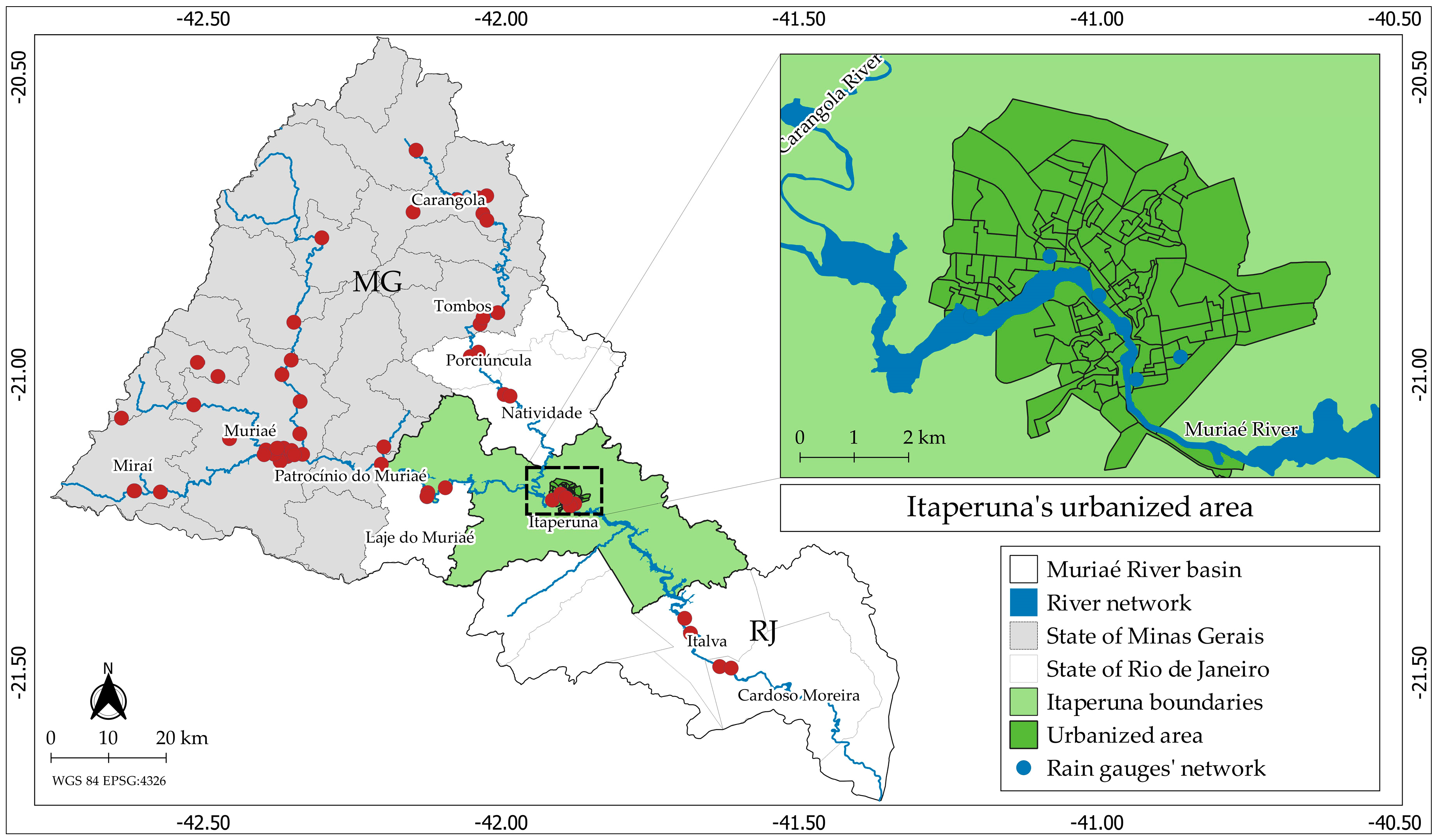
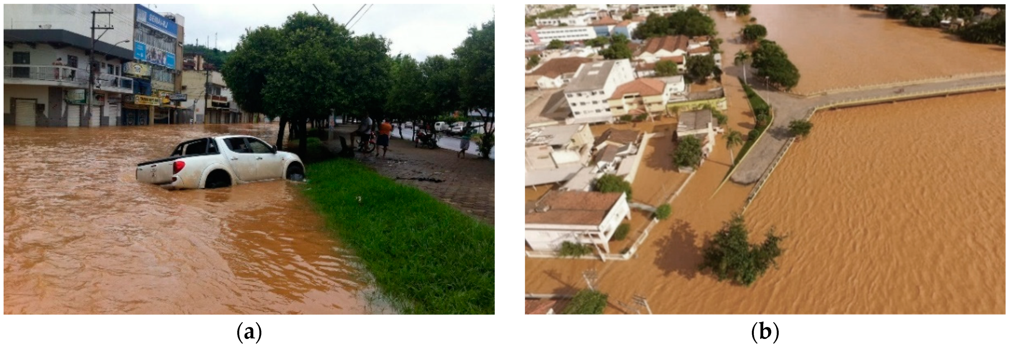
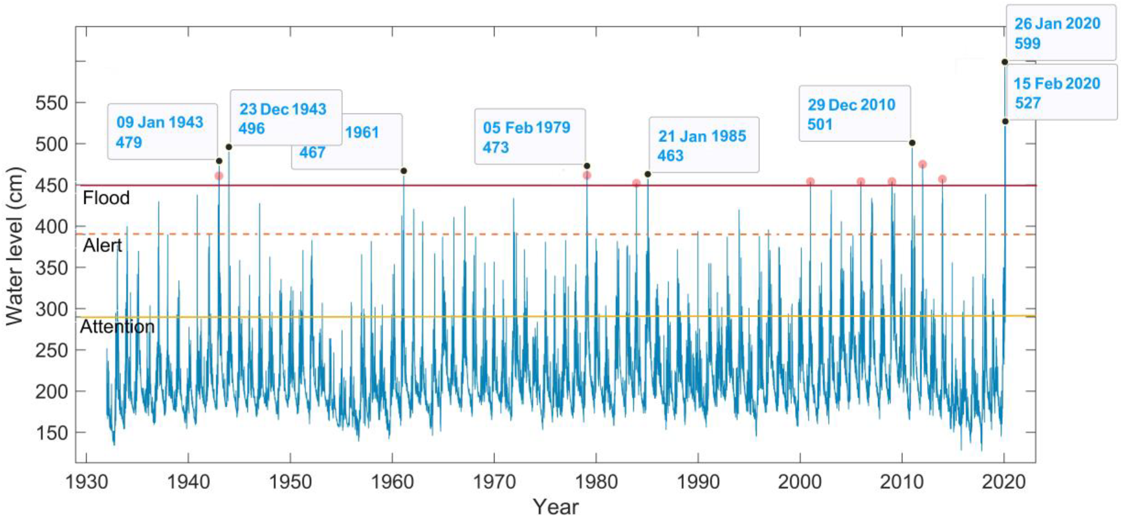
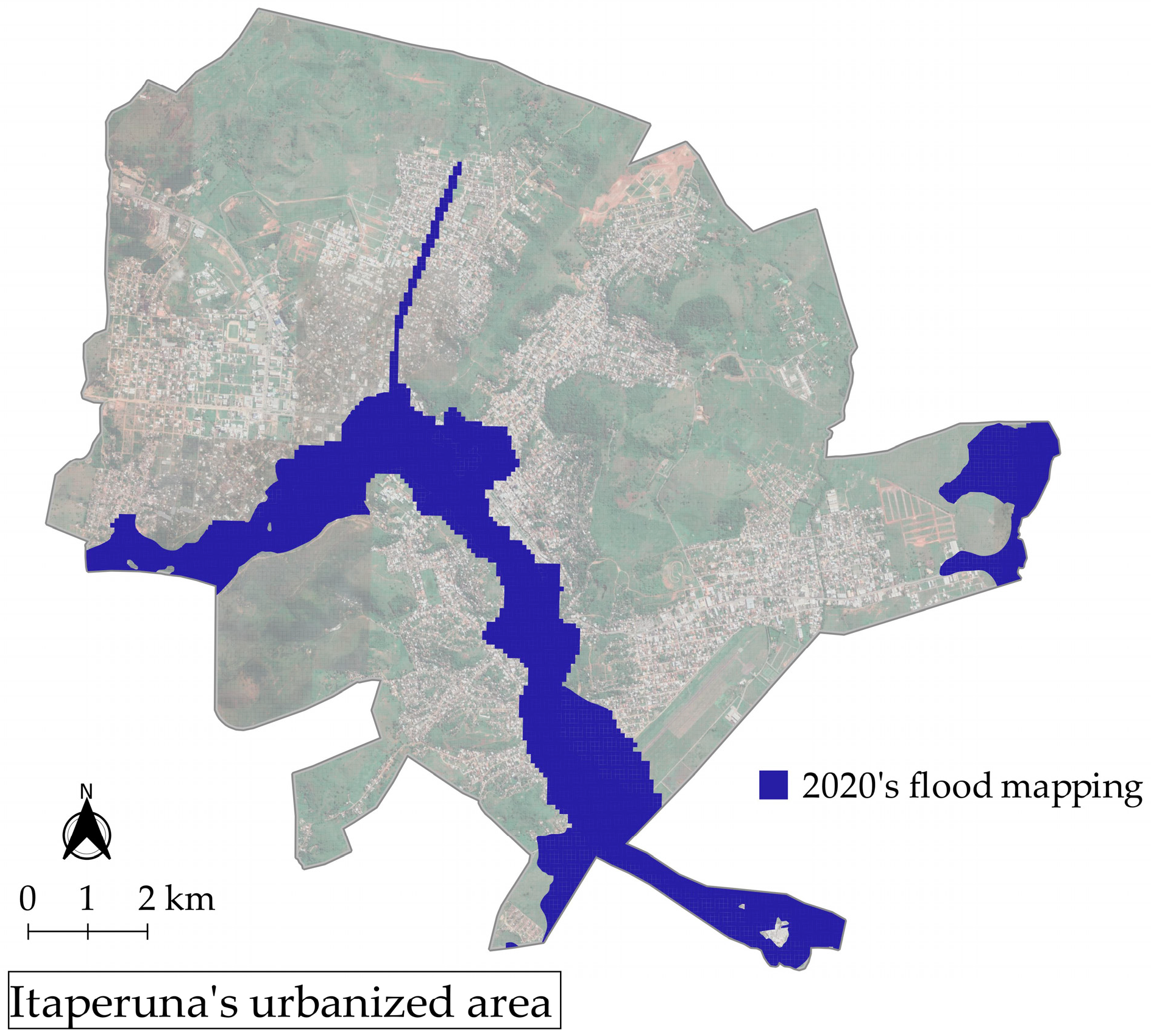
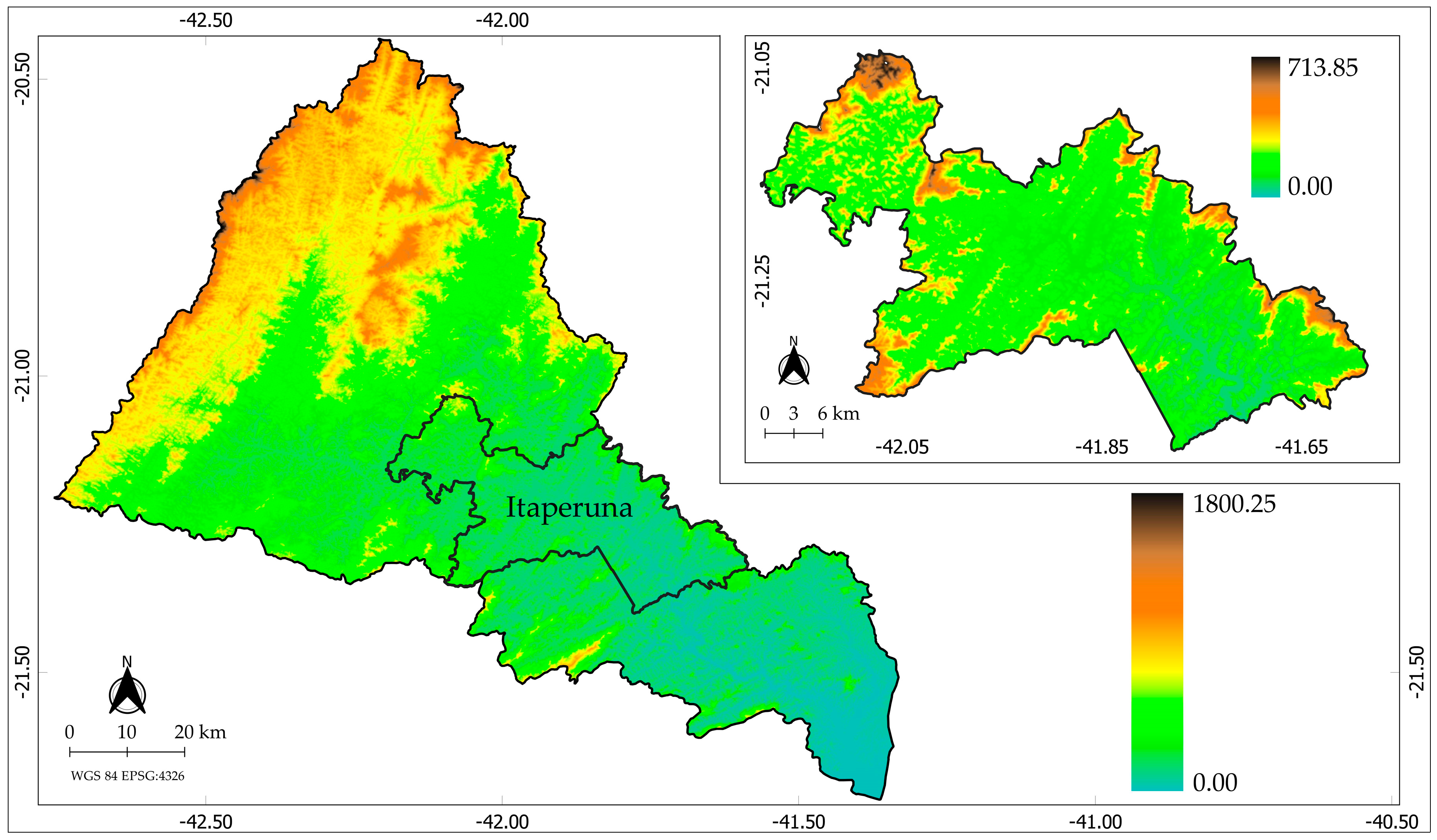
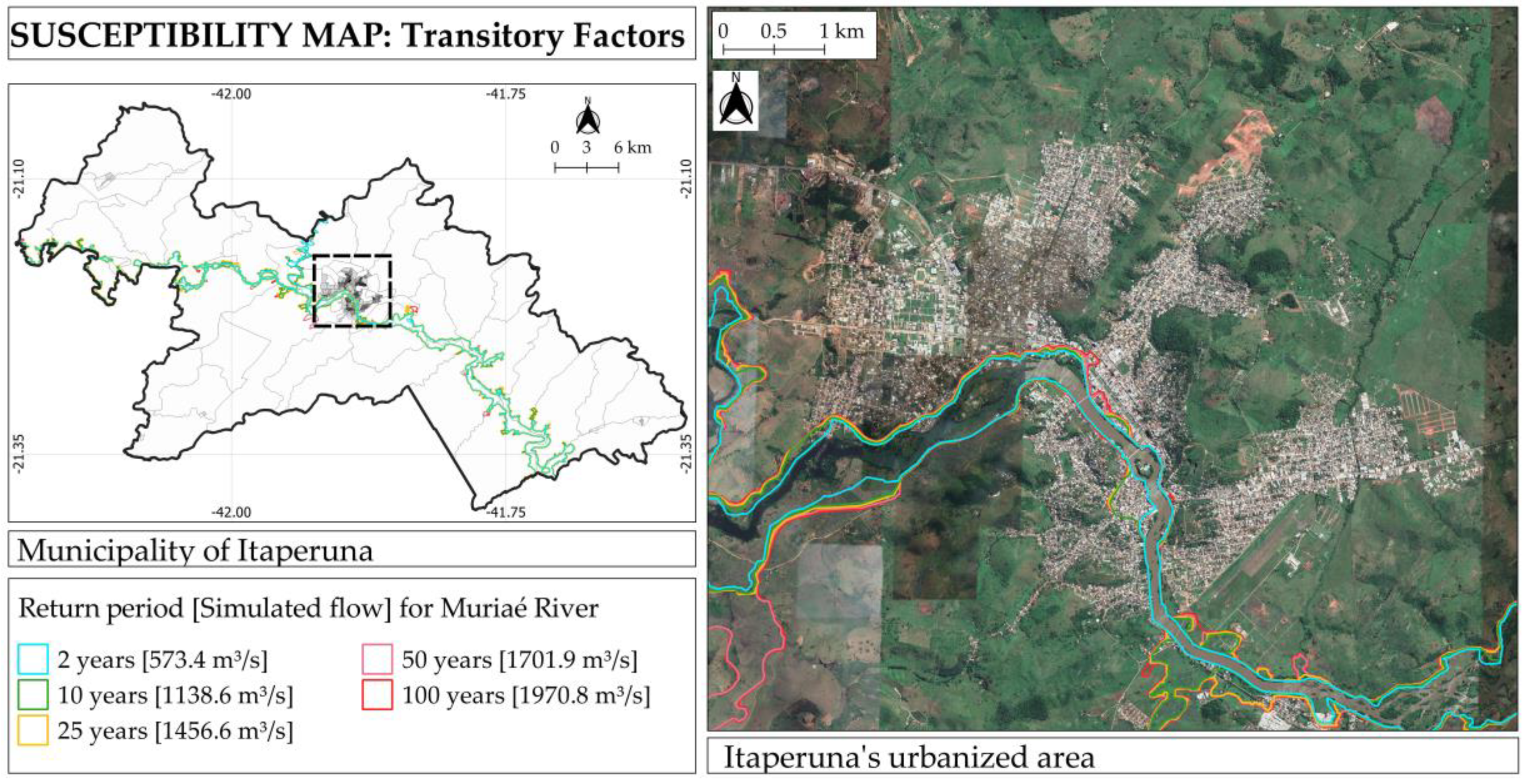
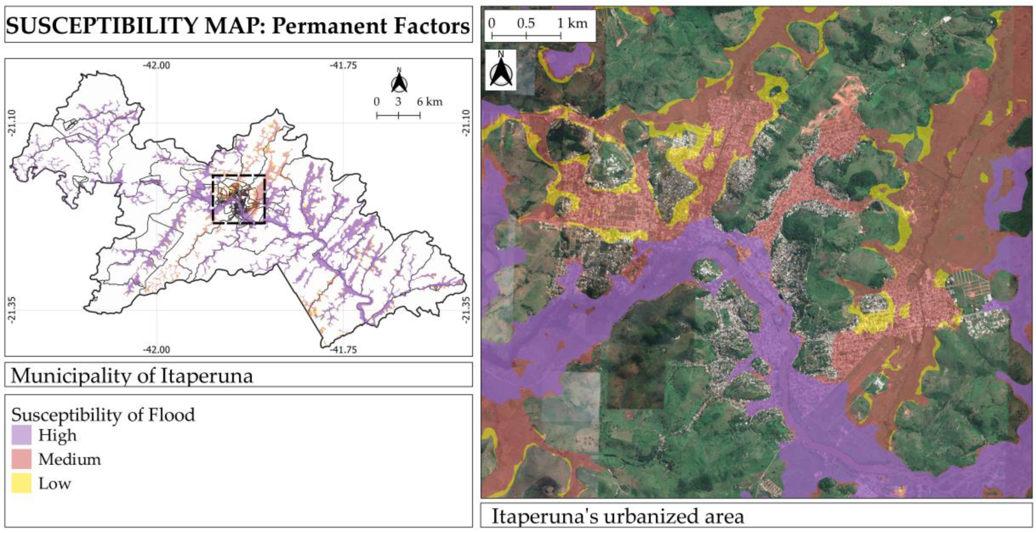
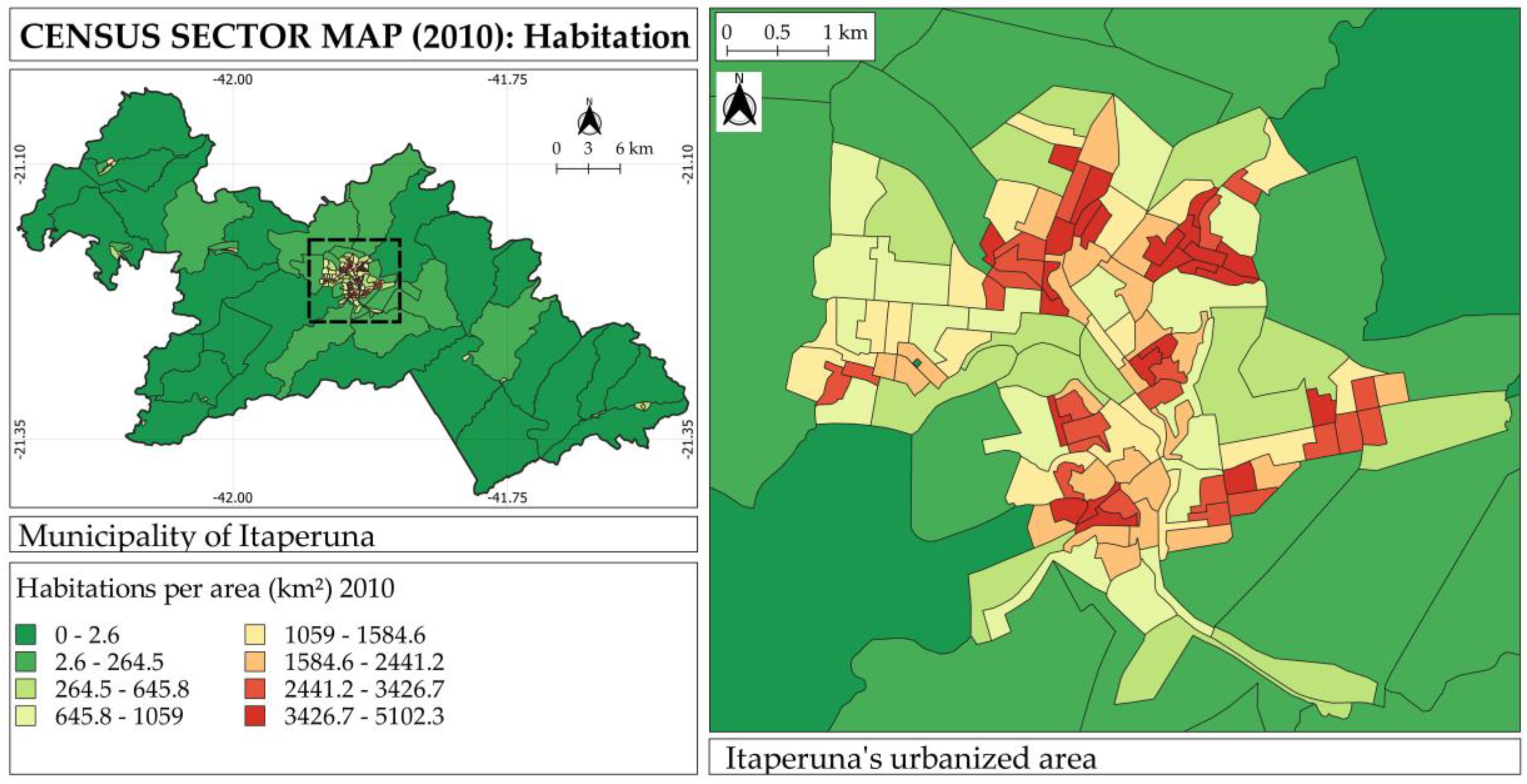
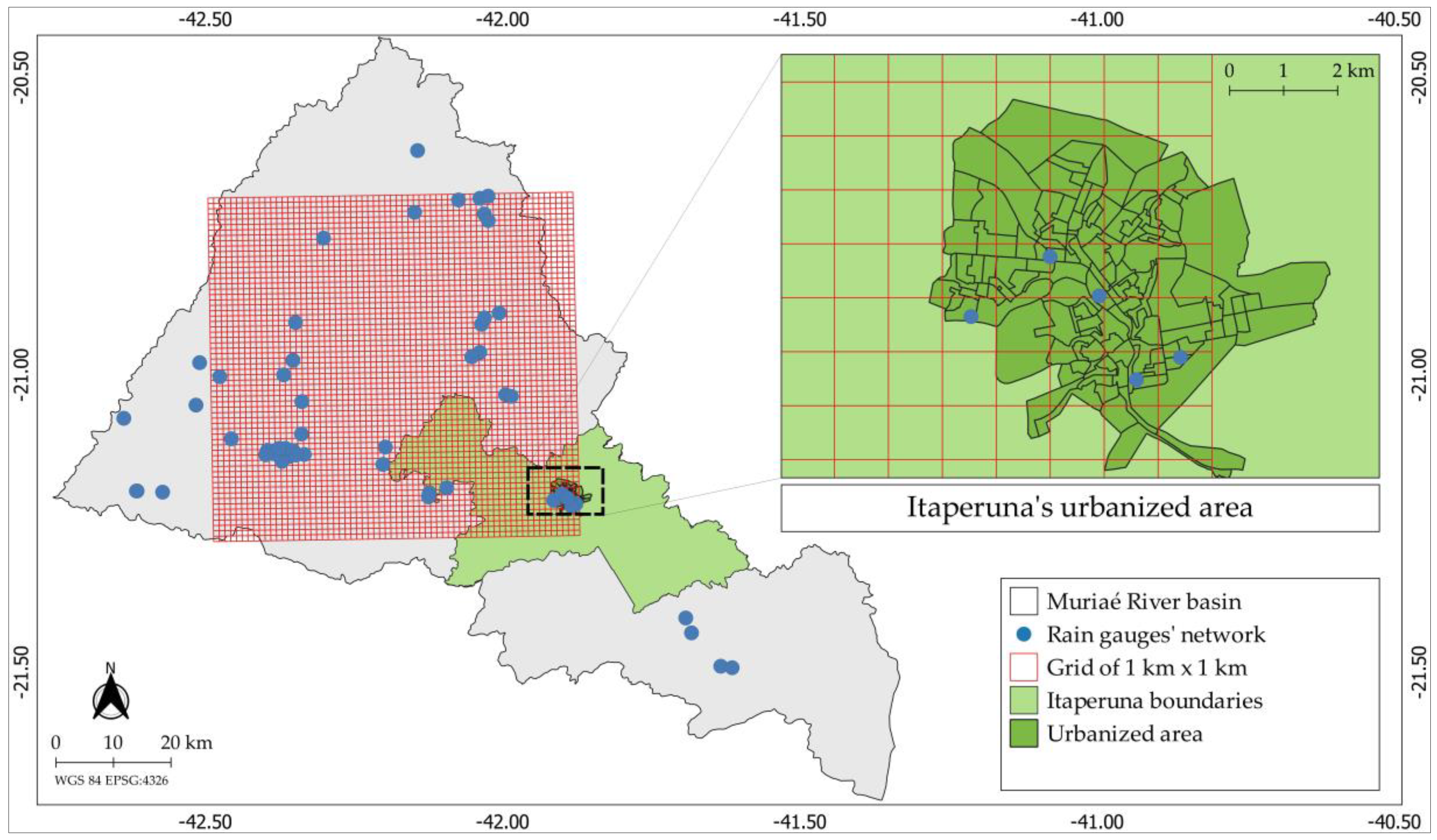
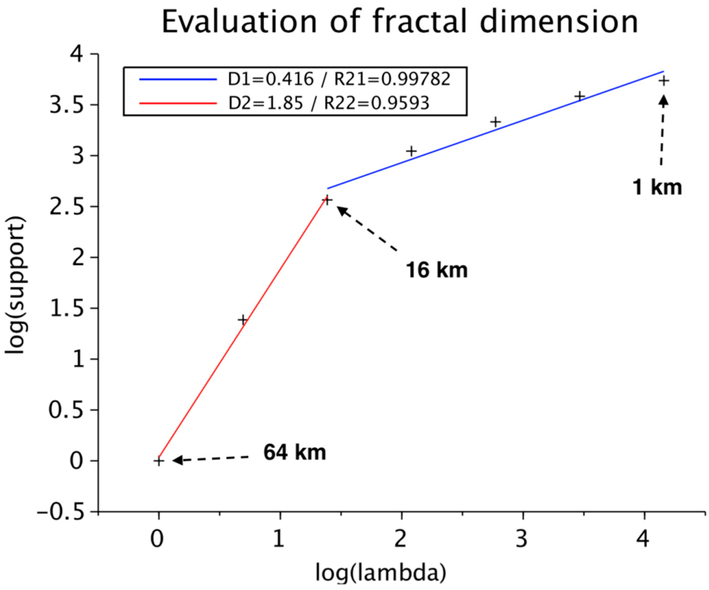
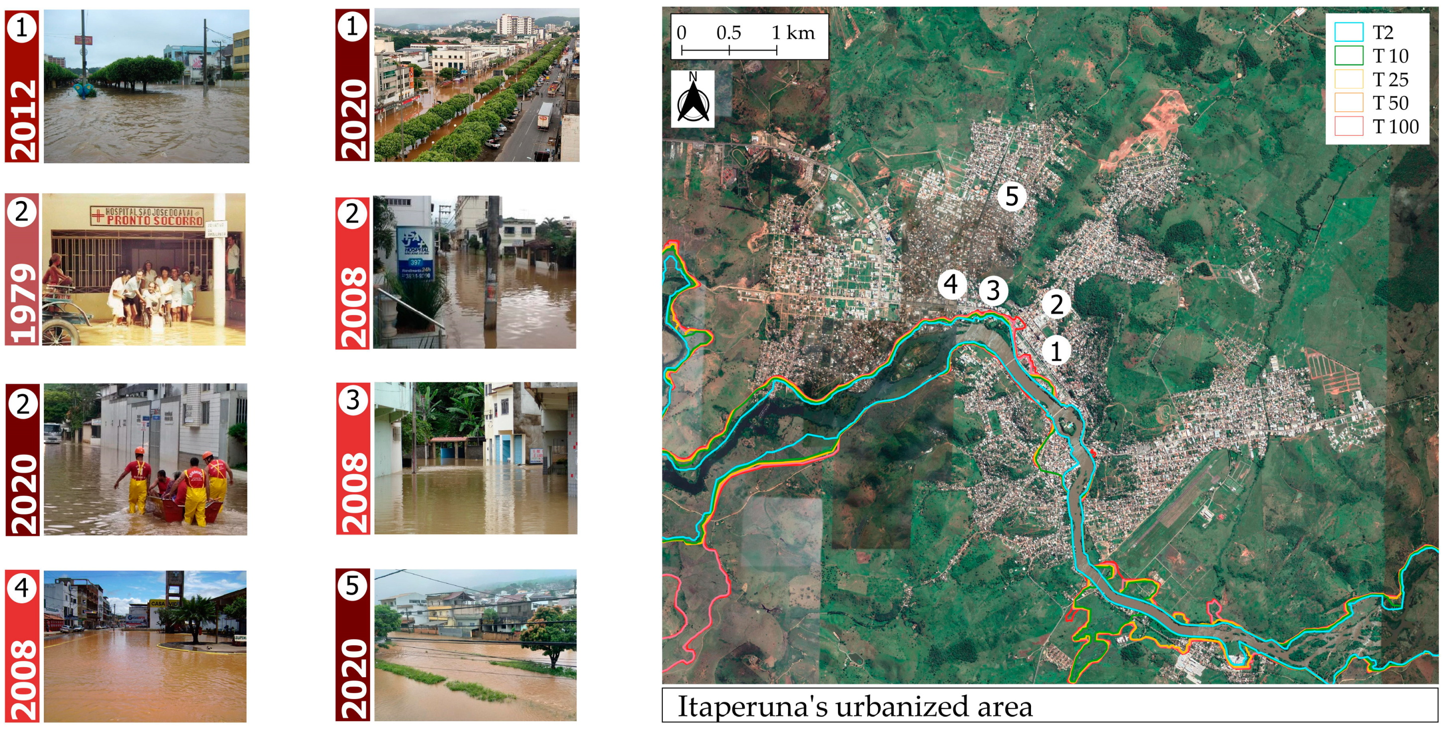
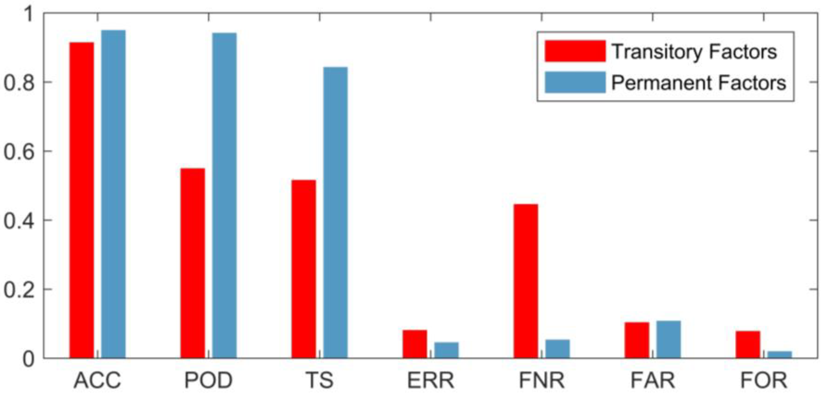
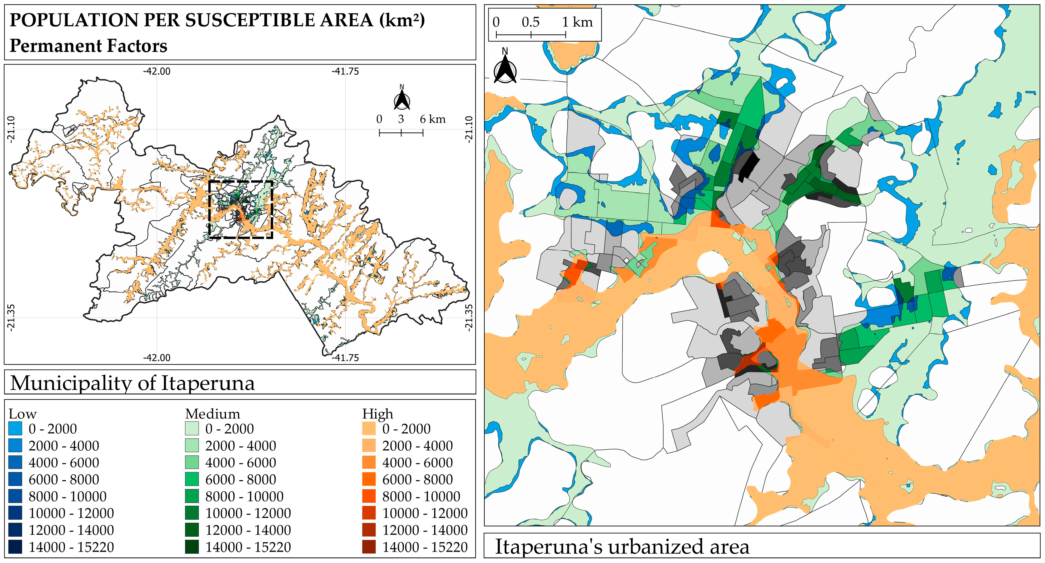
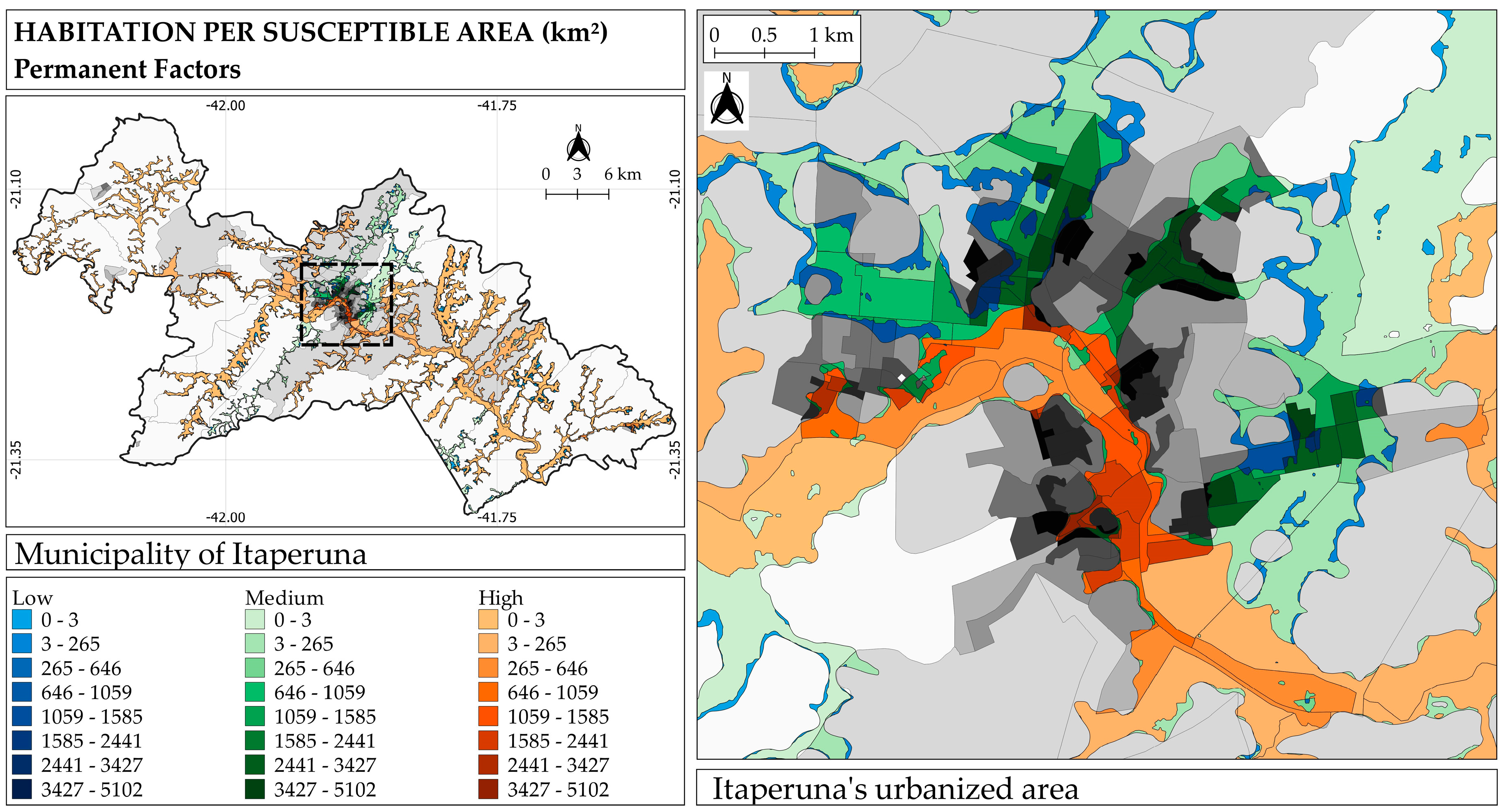
Table 1.
Correlation matrix between Morphometric Indexes and Height Above Nearest Drainage (HAND) Model [62].
Table 1.
Correlation matrix between Morphometric Indexes and Height Above Nearest Drainage (HAND) Model [62].
| Morphometric Indexes\HAND Model | High Susceptibility | Medium Susceptibility | Low Susceptibility |
|---|---|---|---|
| High Susceptibility | High | High | Medium |
| Medium Susceptibility | High | Medium | Low |
| Low Susceptibility | Medium | Low | Low |
Table 2.
Cross-tabulation matrix.
| Predicted 1 | Observations 2 | Row Total | |
|---|---|---|---|
| Positive | Negative | ||
| Positive | TP 3 | FP 5 | TP + FP |
| Negative | FN 4 | TN 6 | FN + TN |
| Column Total | TP + FN | FP + TN | |
1 “Predicted” are associated to the susceptible areas estimated by the flood susceptibility maps based on transitory or permanent factors; 2 “Observations” correspond to the measurement points, i.e., the real occurrences of the event; 3 TP (true positive) means the correct predictions; 4 FN (false negative) means the unannounced events; 5 FP (false positive) means the false warning; 6 TN (true negative) means the correctly predicted non-occurrence.
Table 3.
Cross-Tabulation matrix between the flood susceptibility map based on transitory factors with a return period of 100 years as “predicted” and the recorded data of flood spots measured during the major event of January 2020 as “observations.”
Table 3.
Cross-Tabulation matrix between the flood susceptibility map based on transitory factors with a return period of 100 years as “predicted” and the recorded data of flood spots measured during the major event of January 2020 as “observations.”
| Predicted | Observations | Row Total | |
|---|---|---|---|
| Positive | Negative | ||
| Positive | 2493 | 296 | 2789 |
| Negative | 2024 | 23,042 | 25,066 |
| Column Total | 4517 | 23,338 | |
Table 4.
Cross-Tabulation matrix between the flood susceptibility map considering the high susceptibility based on permanent factors as “predicted” and the recorded data of flood spots measured during the major event of January 2020 as “observations.”
Table 4.
Cross-Tabulation matrix between the flood susceptibility map considering the high susceptibility based on permanent factors as “predicted” and the recorded data of flood spots measured during the major event of January 2020 as “observations.”
| Predicted | Observations | Row Total | |
|---|---|---|---|
| Positive | Negative | ||
| Positive | 7294 | 905 | 8199 |
| Negative | 432 | 19,224 | 19,656 |
| Column Total | 7726 | 20,129 | |
Table 5.
The total number of estimated population and habitations (according to the census of 2010) located in flood-prone areas to be affected by floods with three different degrees of susceptibility: high, medium, and low.
Table 5.
The total number of estimated population and habitations (according to the census of 2010) located in flood-prone areas to be affected by floods with three different degrees of susceptibility: high, medium, and low.
| Census Type | High Susceptibility | Medium Susceptibility | Low Susceptibility |
|---|---|---|---|
| Population | 17,042 | 42,013 | 47,055 |
| Habitation | 5874 | 14,705 | 16,661 |
Table 6.
The total number of estimated population and habitations (according to the census of 2010) to be affected by floods with three different degrees of susceptibility: high, medium, and low.
Table 6.
The total number of estimated population and habitations (according to the census of 2010) to be affected by floods with three different degrees of susceptibility: high, medium, and low.
| Itaperuna’s Zones | Census Type | High Susceptibility | Medium Susceptibility | Low Susceptibility |
|---|---|---|---|---|
| ZRBD | Population | 6638 | 17,873 | 19,031 |
| Habitation | 2238 | 5884 | 6290 | |
| ZRMD | Population | 3687 | 13,909 | 16,879 |
| Habitation | 1257 | 4669 | 5668 | |
| ZC | Population | 1341 | 1750 | 1750 |
| Habitation | 520 | 674 | 674 | |
| ZROR | Population | 336 | 625 | 649 |
| Habitation | 114 | 213 | 221 | |
| ZDI | Population | 11 | 14 | 14 |
| Habitation | 4 | 5 | 5 | |
| ZEDE | Population | 7 | 11 | 18 |
| Habitation | 2 | 4 | 6 | |
| ZEIS | Population | 0 | 496 | 505 |
| Habitation | 0 | 152 | 155 | |
| Rural/District | Population | 5023 | 7336 | 8209 |
| Habitation | 1739 | 3104 | 3642 |
© 2020 by the authors. Licensee MDPI, Basel, Switzerland. This article is an open access article distributed under the terms and conditions of the Creative Commons Attribution (CC BY) license (http://creativecommons.org/licenses/by/4.0/).
Share and Cite
MDPI and ACS Style
Campos, P.C.d.O.; Paz, I. Spatial Diagnosis of Rain Gauges’ Distribution and Flood Impacts: Case Study in Itaperuna, Rio de Janeiro—Brazil. Water 2020, 12, 1120. https://doi.org/10.3390/w12041120
AMA Style
Campos PCdO, Paz I. Spatial Diagnosis of Rain Gauges’ Distribution and Flood Impacts: Case Study in Itaperuna, Rio de Janeiro—Brazil. Water. 2020; 12(4):1120. https://doi.org/10.3390/w12041120
Chicago/Turabian StyleCampos, Priscila Celebrini de Oliveira, and Igor Paz. 2020. "Spatial Diagnosis of Rain Gauges’ Distribution and Flood Impacts: Case Study in Itaperuna, Rio de Janeiro—Brazil" Water 12, no. 4: 1120. https://doi.org/10.3390/w12041120
Note that from the first issue of 2016, this journal uses article numbers instead of page numbers. See further details here.