Analysis of Climate Change’s Effect on Flood Risk. Case Study of Reinosa in the Ebro River Basin


Department of Geotechnical Engineering, Universitat Politècnica de València, 46022 Valencia, Spain
*
Author to whom correspondence should be addressed.
Water 2020, 12(4), 1114; https://doi.org/10.3390/w12041114
Submission received: 27 February 2020
/
Revised: 2 April 2020
/
Accepted: 7 April 2020
/
Published: 14 April 2020
(This article belongs to the Special Issue Flood Risk Assessments: Applications and Uncertainties)
Abstract
:Floods are one of the natural hazards that could be most affected by climate change, causing great economic damage and casualties in the world. On December 2019 in Reinosa (Cantabria, Spain), took place one of the worst floods in memory. Implementation of DIRECTIVE 2007/60/EC for the assessment and management of flood risks in Spain enabled the detection of this river basin with a potential significant flood risk via a preliminary flood risk assessment, and flood hazard and flood risk maps were developed. The main objective of this paper is to present a methodology to estimate climate change’s effects on flood hazard and flood risk, with Reinosa as the case study. This river basin is affected by the snow phenomenon, even more sensitive to climate change. Using different climate models, regarding a scenario of comparatively high greenhouse gas emissions (RCP8.5), with daily temperature and precipitation data from years 2007–2070, and comparing results in relative terms, flow rate and flood risk variation due to climate change are estimated. In the specific case of Reinosa, the MRI-CGCM3 model shows that climate change will cause a significant increase of potential affected inhabitants and economic damage due to flood risk. This evaluation enables us to define mitigation actions in terms of cost–benefit analysis and prioritize the ones that should be included in flood risk management plans.
1. Introduction
Floods are natural hazards that produce great material damage and human losses worldwide [1]. The increasing population density and infrastructure on river banks contribute to increased floodplain vulnerability, which can result in severe social, economic and environmental damage [2].
The fourth of the nine essential rules of flood risk management indicates that it should be taken into account that “The future will be different from the past. Climate and societal change as well as changes in the condition of structures can all profoundly influence flood risk” [3].
For all these reasons, it is essential to design methodologies that enable one to estimate flow regime variations and evaluate flood risk modification due to climate change. [4,5,6].
The technical document of the IPCC IV forecasts a probable increase in the frequency and intensity of precipitation episodes, as well as a decrease in average values in summer for mid-latitudes countries as Spain. The Fifth Assessment Report (AR5) of the IPCC (2013–14), points out that it is probable that the frequency or intensity of intense rainfall has increased in Europe, and in relation to future changes, that extreme precipitation events over most of the mid-latitude lands will most likely be more intense and more frequent [7]. Additionally, climate change can specially affect those regions in which the snow phenomenon is relevant in hydrological behavior.
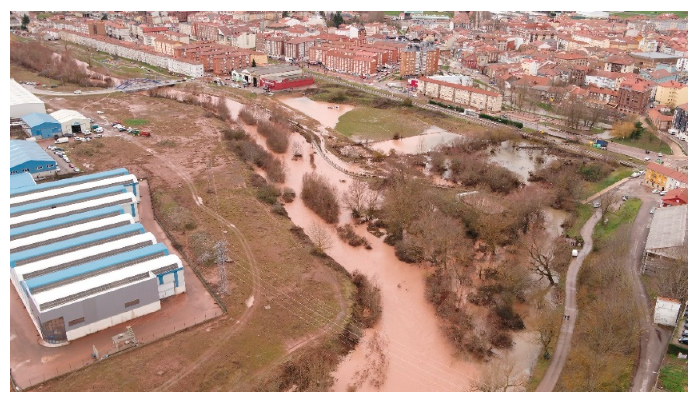
As a matter of these facts, the 2019 flash flood European notifications beat the last 7 years of notifications clearly [8], and Reinosa (Cantabria, Spain) suffered two important floods on January and December 2019, the second one being one of the worst floods in memory. This flood was caused by the Elsa storm, on December 19 and 20, which came from the southwest and was accompanied by very strong winds and very high temperatures for that time of the year, causing the melting of the snow-cover in the highest part of the catchment. A203 gauging station, recorded on 20 December 2019 at 1:00 a.m., 246 m3/s instant (15 minutes period) flow, while the maximum ever recorded was 100 m3/s (27 February 2010). The daily flow rate recorded by A203 for this event was 83 m3/s and the return period has been estimated approximately as Tr = 300 years. This flood caused great damage in Reinosa, affecting residential areas (Figure 1).
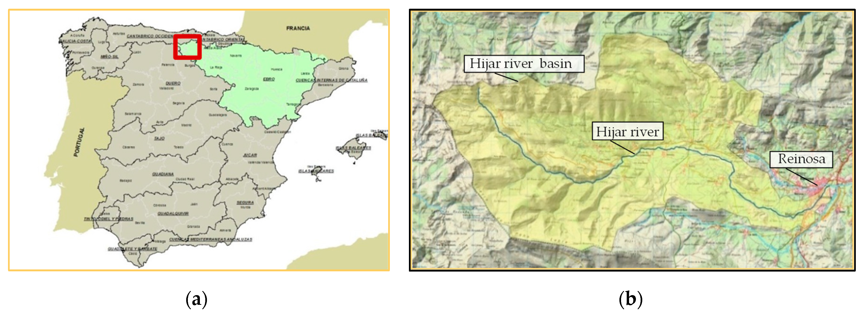
Reinosa (Cantabria, Spain) is located in the north of the Iberian Peninsula, in the junction of Hijar, Ebro and Izarilla rivers, immediately upstream the Ebro reservoir. Hijar catchment, with 27.6 km length and 147.6 km2 surface, drains the highest area of Cantabrian mountain range that belongs to the Ebro river basin. The catchment height ranges between 865 and 2023 m above sea level, with a mean height of 1351 m. A203 gauging station is located in Hijar River, immediately upstream of Reinosa, with a time of concentration of approximately 15 hours.
The average rainfall of the head of the Ebro for the period 1920–2002 was 1190 mm/year, concentrated in autumn and winter, characteristic of an Atlantic climate, with some continental patterns producing 33 L/s/km2. The average annual temperature is 8.9 °C in Reinosa. The main land uses in the catchment are forest and scrub. Figure 2 shows Hijar river basin overall and site map.
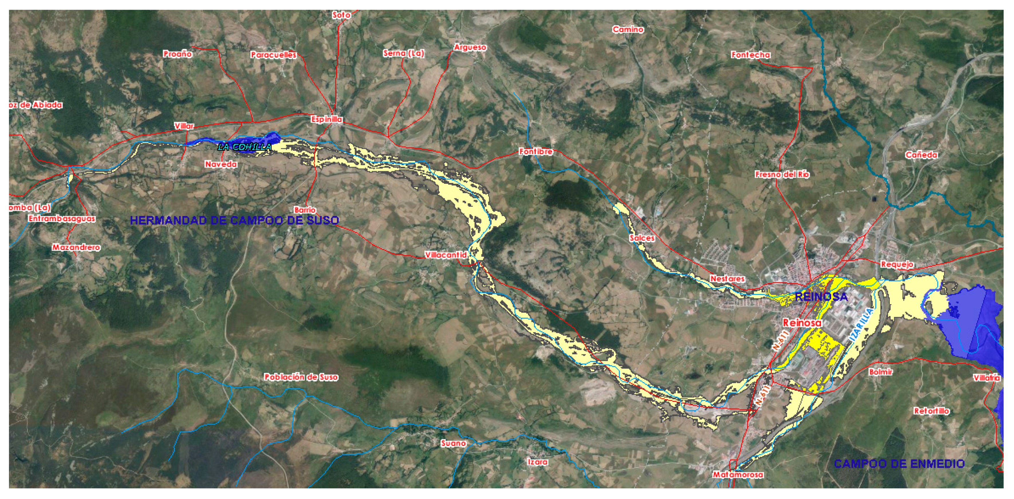
Reinosa belongs to the Hijar river basin, and had potential significant flood risk (ES091_HIJ_01_02_04_05_06) during the implementation of DIRECTIVE 2007/60/EC, as shown in Figure 3.
DIRECTIVE 2007/60/EC implies an objective quantification of flood risk, for low (500 years return period), medium (100 years return period) and high probabilities (10 years return period), that will allow the efficient development of flood risk management plans by implementing a set of combined actions to reduce floods’ consequences [9].
To evaluate different climate change scenarios, the Spanish Meteorological Agency (AEMET) regionalized a set of global climate models, by using two statistical downscaling methods. The usefulness of this regionalization was assessed by their fitting to the observed data in the control period (1961–2000). A comparison based on a set of statistics show that although the fit is good for annual mean values, annual maximum values for both regionalization methods are not adequately simulated, since they provide lower extremes with a smaller variability. However, different fitting was observed depending on the Spanish region [10].
Although results might show a decrease in the magnitude of extreme floods for climate model projections downscaled by AEMET [11], a different pattern might be concluded, when taking into account snowmelt, if the melting flow rate’s increase due to higher temperatures is bigger than the decrease caused by less snow accumulation.
The main aim of the work is to estimate flow and flood risk variation due to climate change by using different climate models regarding a scenario of comparatively high greenhouse gas emissions (RCP8.5), with daily temperature and precipitation data.
2. Materials and Methods
2.1. Overall Methodology
According to DIRECTIVE 2007/60/EC, Spanish hazard and flood risk maps can be downloaded at https://sig.mapama.gob.es/snczi/, regarding the following scenarios: (a) floods with a low probability, or extreme event scenarios (return period ≥ 500 years); (b) floods with a medium probability (likely return period ≥ 100 years); (c) floods with a high probability (return period ≥ 10 years).
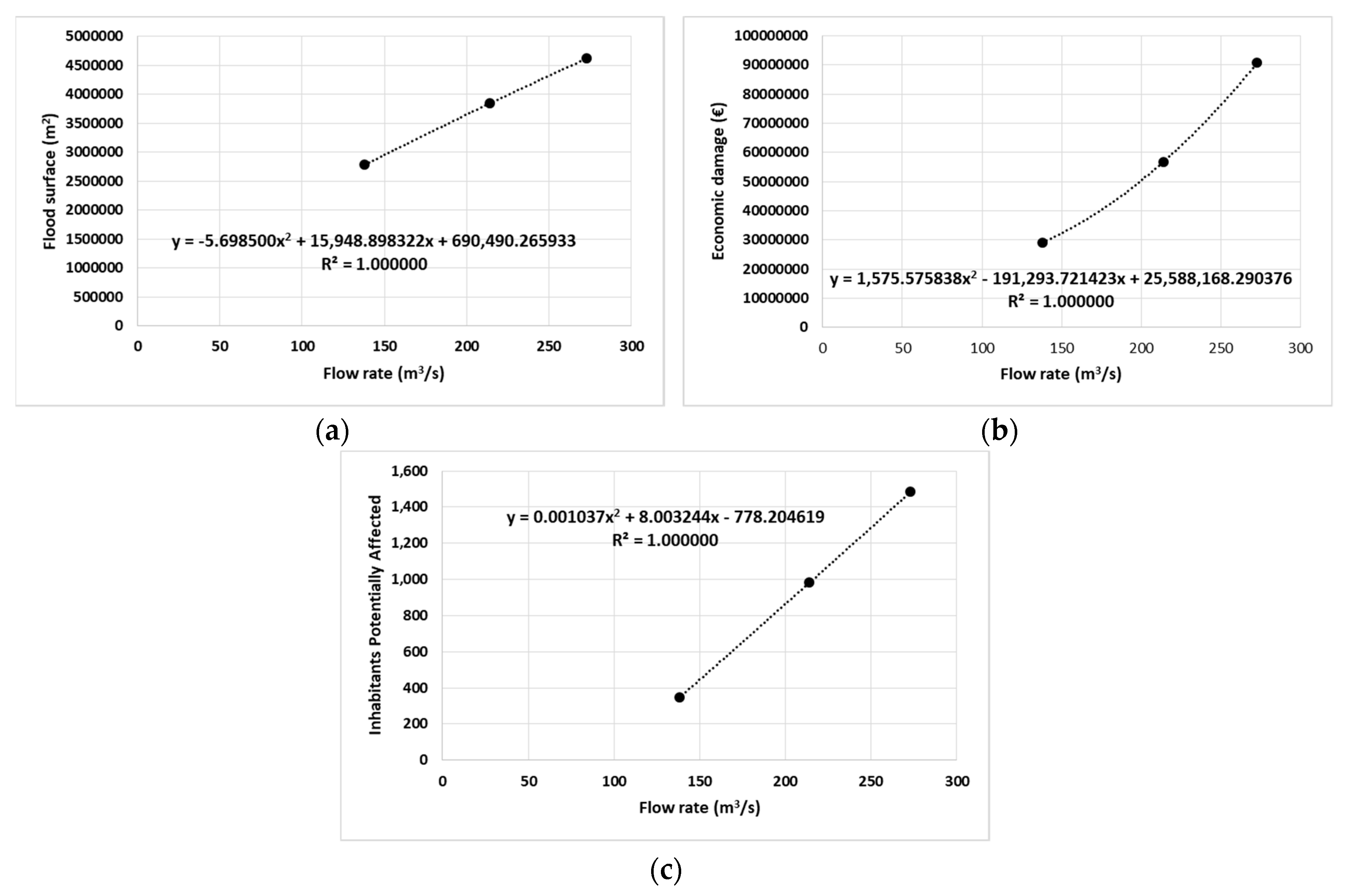
By relating flow rates in A203 gauging station with hazard and risk maps, correlations with flooding surface, economic damage and casualties can be achieved.
In order to evaluate climate change, projections of a series of climatic variables are entered as input data in a calibrated hydrological model in the study basin. The ASTER® model is a distributed hydrological model that calculates snowmelt and accumulation regarding energy balance [12,13]
Two global climate models (GCM), downscaled by the Spanish Meteorological Agency (AEMET), have been selected; we validated them with real flow rates from the control period (1961 to 2000) and used under the highest greenhouse gas emissions pathway (RCPs 8.5) from the Fifth Assessment Report of the Intergovernmental Panel on Climate Change.
The relationship between calculated daily flow rates and instant (15 minutes period) flow rates is not necessary for these downscaled climate models, as climate change’s effect will be calculated in relative terms comparing climate models in the calculation period in two equal length stages (2007–2038) and (2039–2070).
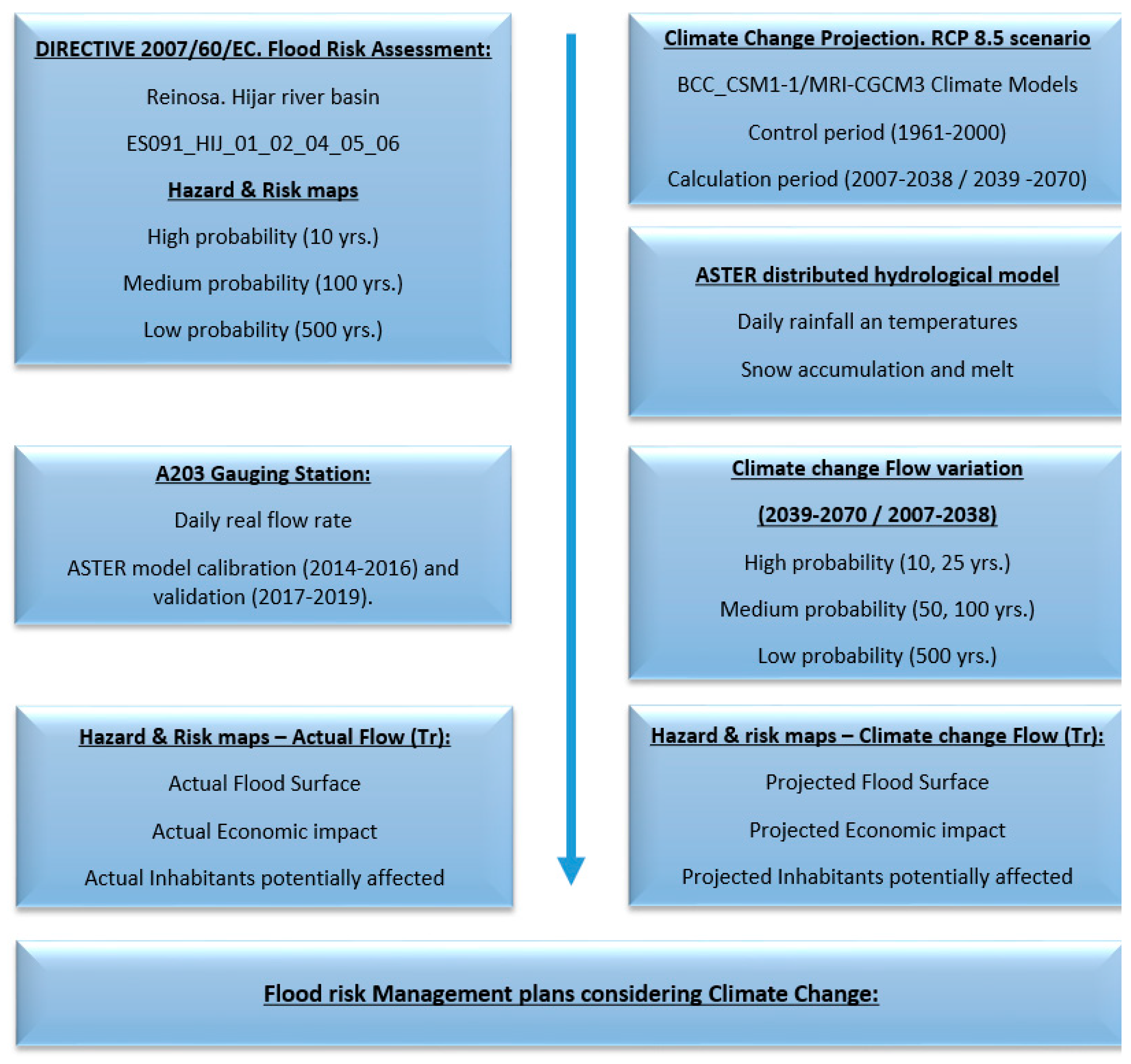
Once the flow rate variation for the climate projection is estimated and applied on real flow, new impacts on hazard and risk maps can be established. Figure 4 shows the overall methodology scheme.
2.2. Hazard and Risk Maps
Hazard maps are the result of two-dimensional hydraulic models, indicating flooded area, flood depths and flood velocities. Return periods were given by Spanish Authority in the framework of DIRECTIVE 2007/60/EC implementation by “Maximum Flow Maps” software, based on a regionalized gauging station study [14].
Flood risk maps shall show the potential adverse consequences associated with flood scenarios, and express, among other things, terms of the indicative numbers of inhabitants potentially affected and the type of economic activity of each area potentially affected. Additionally, economic damage can be estimated.
According to DIRECTIVE 2007/60/EC, these maps serve as a tool for establishing priorities and for making additional technical, economic and political decisions related to flood risk management. Measures to be implemented in the at-risk areas can be prioritized, depending on the results of the cost-benefit analysis. They also allow us to evaluate climate change’s effects. The risk associated with flood events is established based on the vulnerability of the threatened element and the hazard to which it is exposed. The estimation of indicative number of inhabitants potentially affected depends on updated census data. The Spanish Water Authority has also established a methodology to estimate the economic value of flood damage partially based on the PREEMPT project [15,16].
2.3. Hydrological Model
2.3.1. Hijar Basin Model
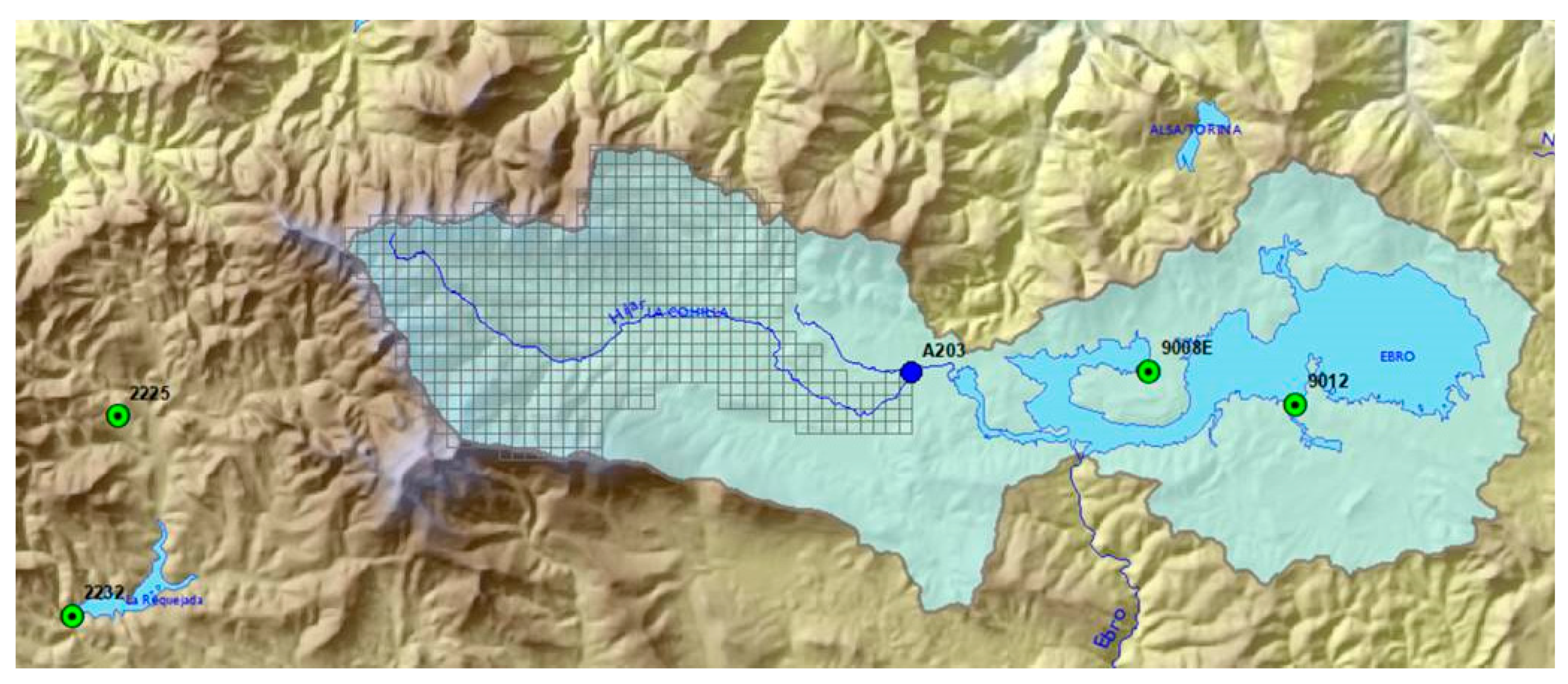
A 500 by 500 m grid and daily time resolution distributed hydrological model has been built for the Hijar river basin (Figure 6), with A203 gauging station in Reinosa as the outlet and calibration point, 2014–2016 as the calibration period and 2017–2019 as the validation period.
ASTER® is a distributed hydrological model that calculates streamflow in a river using rainfall, temperature, windspeed and radiation as climate inputs. It has been applied in several countries and implemented by Spanish water authorities as an accurate model in river basins with strong snow phenomena, as in our case study (Hijar catchment) [17,18]. Figure 7 shows the snow–water equivalent for two consecutive days in Hijar model.
2.3.2. Snow Accumulation Routine
Precipitation will be snow or water form at different temperatures depending on several atmospheric conditions. This range of temperatures can vary between −2 and 2 °C. The model sets a temperature, named rain/snow temperature, at which 50% of precipitation is snow, with a bilineal increase and decrease of snow form up to −2 and 2 °C.
2.3.3. Snowmelt Routine
As aforementioned, snowmelt is calculated using the energy balance equation. Melting takes place when air temperature is below a specific temperature (—snowmelt temperature). Snowmelt can be divided into two types: (a) rainfall snowmelt; (b) no rainfall snowmelt.
Rainfall Snowmelt
It is the snowmelt produced by rainfall energy. Assuming that the snow surface temperature is equal to 0 °C (273 K), snowmelt caused by energy from rainfall is [19]:
where:
In addition to energy from rainfall, other secondary terms as radiation and condensation energy must be added to calculate snowmelt when rain takes place.
No Rainfall Snowmelt
It is the snowmelt on a dry day. Due to difficulties estimating wind speed, hydrological models usually use non-forced convection or other empirical relations depending on air temperature. The following equation is used to estimate no rainfall melt [20]:
where:
This melt factor ( indicates the seasonal variation, and can be represented with a sine function [21,22].
where:
- .
2.3.4. Model Calibration and Validation
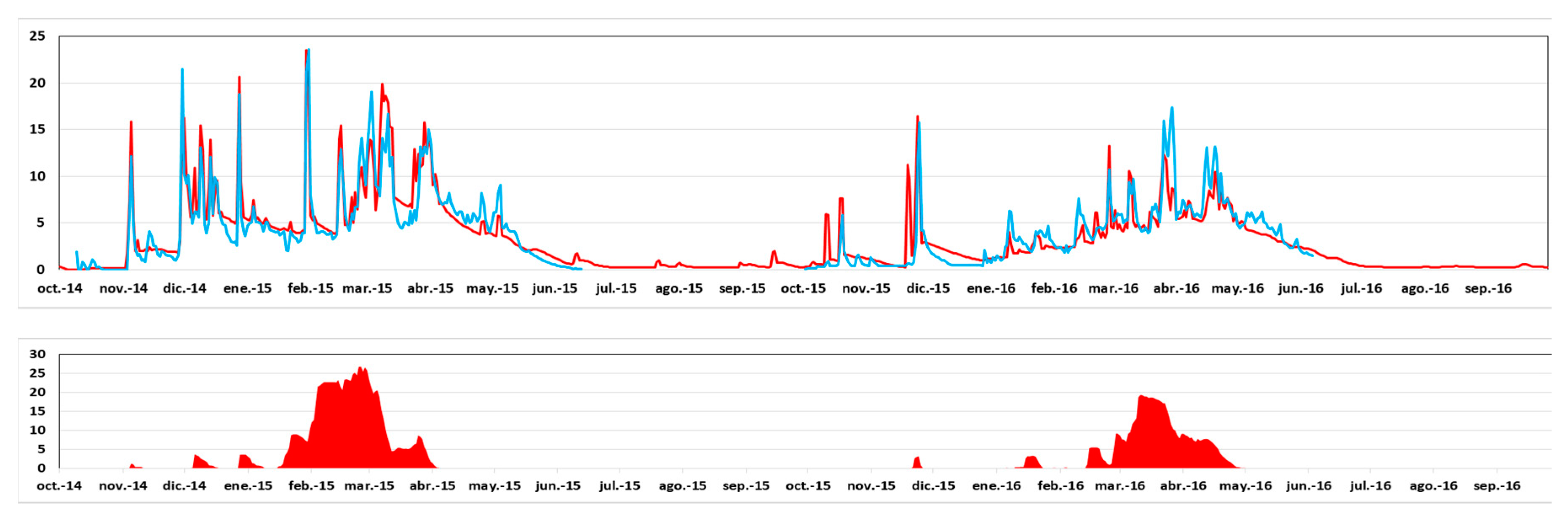
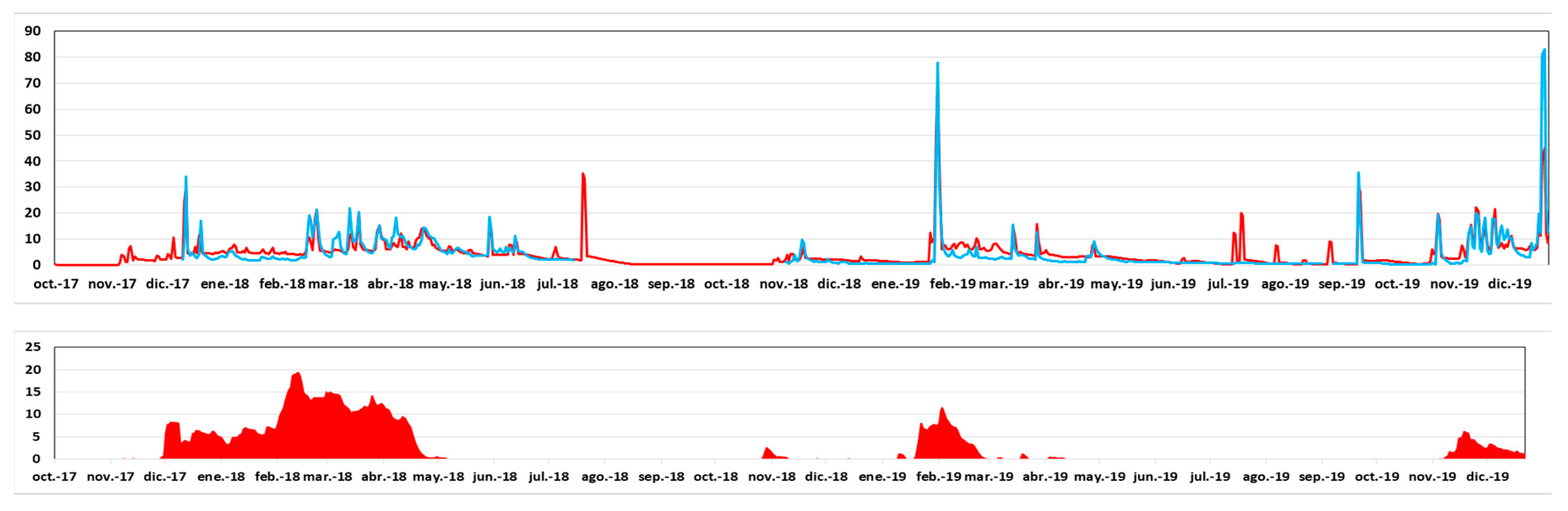
Calibration and validation have been carried out, comparing real daily flow rates, in A203 Hijar in Reinosa Gauging Station with the ASTER model daily flow rates being calculated with real meteorological data. The available continuous period for the observed daily flow rate ranges from 2014 to 2019, defining the calibration period as October 1st 2014 to September 30th 2016 and the validation period from October 1st 2017 to December 22nd 2019, including the aforementioned extraordinary event.
Figure 8, shows results during the calibration period, with a correlation coefficient of 0.90 and a Nash index (NSE) of 0.78. The maximum observed daily flow rate was 23.6 m3/s, and the maximum calculated daily flow rate was 23.5 m3/s. Total observed runoff was 189 hm3 and calculated runoff was 200.7 hm3, with 27 hm3 of overall snow–water equivalent accumulation.
The main calibration parameters of the model are:
- MFMAX = 5.5 (mm/°C/24 h);
- MFMIN = 1.46 (mm/°C/24 h);
- Tmi = −0.35 (°C);
- Rain/Snow temperature = −0.53 (°C);
- Altimetry temperature gradient = −3.1 (°C/1000 m).
Figure 9 shows results during the validation period, with a correlation coefficient of 0.90 and a Nash index (NSE) of 0.80. The maximum observed daily flow rate was 83 m3/s, and the maximum calculated daily flow rate was 69 m3/s. Total observed runoff was 231 hm3 and calculated runoff was 289 hm3, with 20 hm3 of overall snow–water equivalent accumulation.
2.4. Climate Projection
Daily rainfall and temperature data from two regionalized climate models (analog method—ANA and statistical regionalization method—SDSM) can be obtained from AEMET website (http://www.aemet.es/es/serviciosclimaticos/cambio_climat) for RCP 8.5.
Two climate models have been selected from 24, to analyze the combination of rainfall and temperature:
- ANA—BCC-CSM1-1-m (BCC);
- ANA—MRI-CGCM3 (MRI).
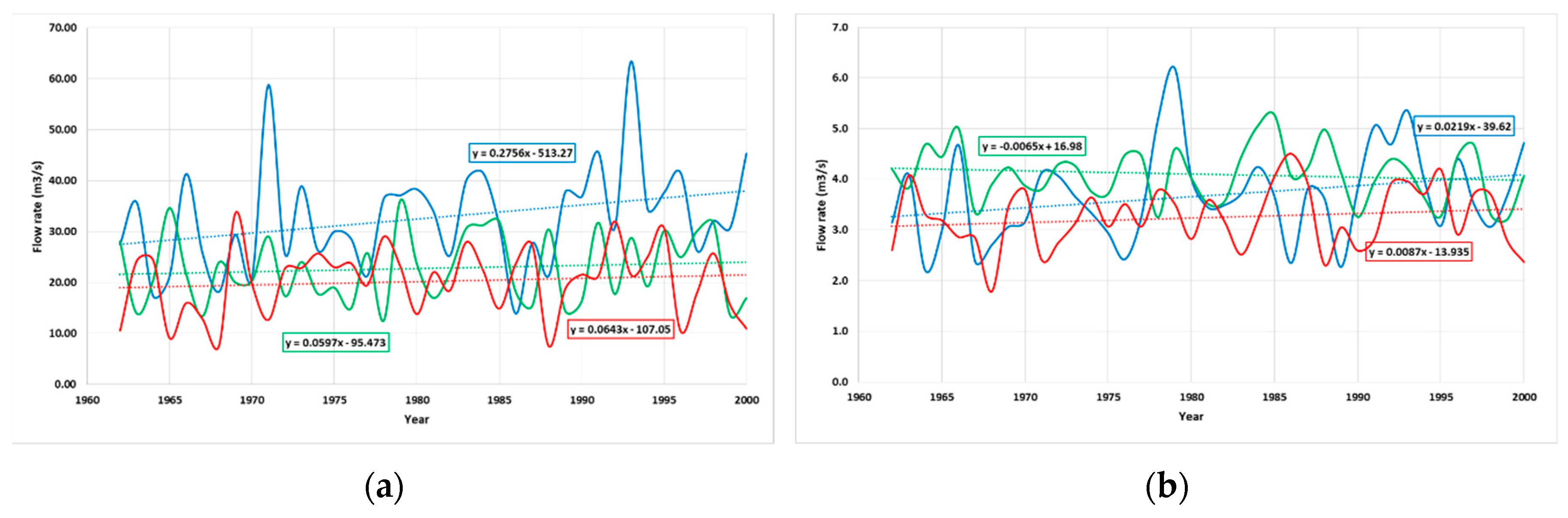
These two models have been pre-selected as generating the highest rainfalls. To evaluate their suitability, daily flow rates for the control period (1961–2000) have been calculated with ASTER for real meteorological data and both climate models. Figure 10a shows that annual maximum real daily flow rates are above climate models, and the trend line shows a higher increase as well. Figure 10b shows that annual mean real daily flow rates fit the MRI better at the beginning of the control period, while a fit better with BCC is shown at the end of the control period. Supplementary Materials for rainfall stations (9008E, 9012) and temperature stations (2225, 2232) is given.
2.5. Calculation of Flow Rates for Different Return Periods
Daily flow rates for the calculation period (2007 to 2070) have been estimated with ASTER model for both climate projections (BCC and MRI). Calculation period has been divided in two equal length stages (2007 to 2038) and (2039–2070) and a probability distribution of extreme values has been estimated using the Gumbel distribution, presenting the best fit goodness:
where:
- u = location parameter;
- β = scale parameter;
- Tr = Return period.
Finally, daily flow rates and instant (15 minute period) flow rates observed in A203 can be fitted in a linear relationship. As climate projections flow rates are being studied in relative terms with observed flow rates, transformation from daily flow rates into instant flow rates is not necessary.
3. Results
3.1. Flow Rate Evolution (RCP 8.5)
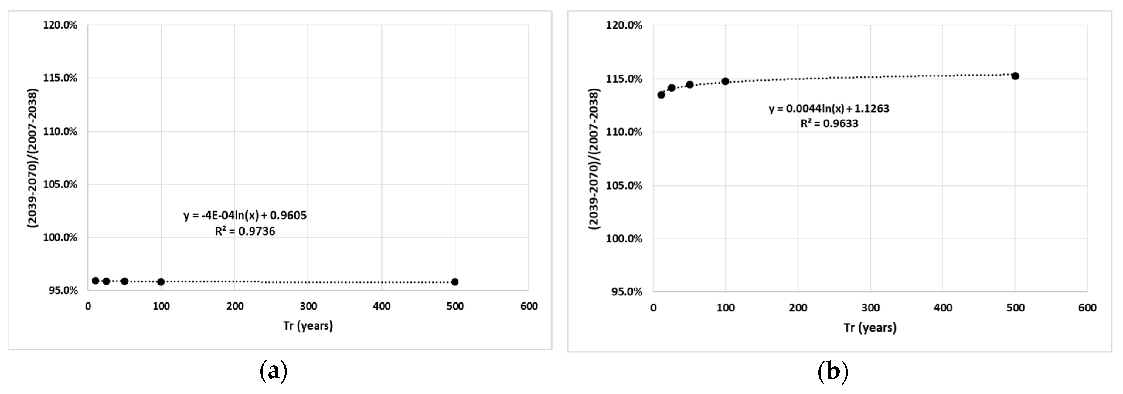
Table 2 and Figure 11 show results and trend lines from percentile analysis for both calculated climate models. For BCC-CSM1-1-m a small decrease in flow rate projection due to climate change is estimated, with small variability for different probabilities, while for MRI-CGCM3 bigger increase is predicted, showing a smooth variability for different probabilities, describing a more extreme climate.
3.2. Hazard and Risk Maps
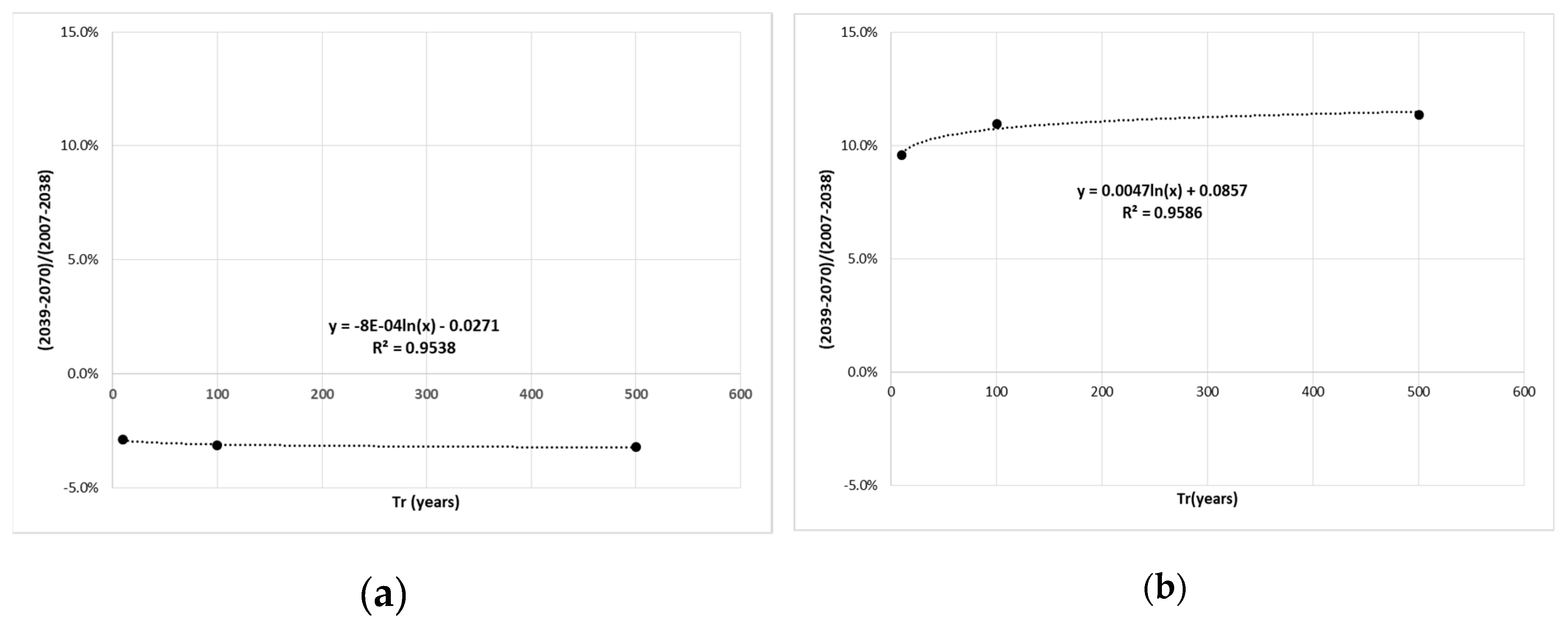
After calculating the projected flow rate by entering for each return period (2nd Stage (2039–2070)/1st Stage (2007–2038)) the flow rate ratio in the trend line fitted for flood surface, economic damage and inhabitants potentially affected (Figure 5), new climate change estimations show similar results as for flow rate (Table 3).
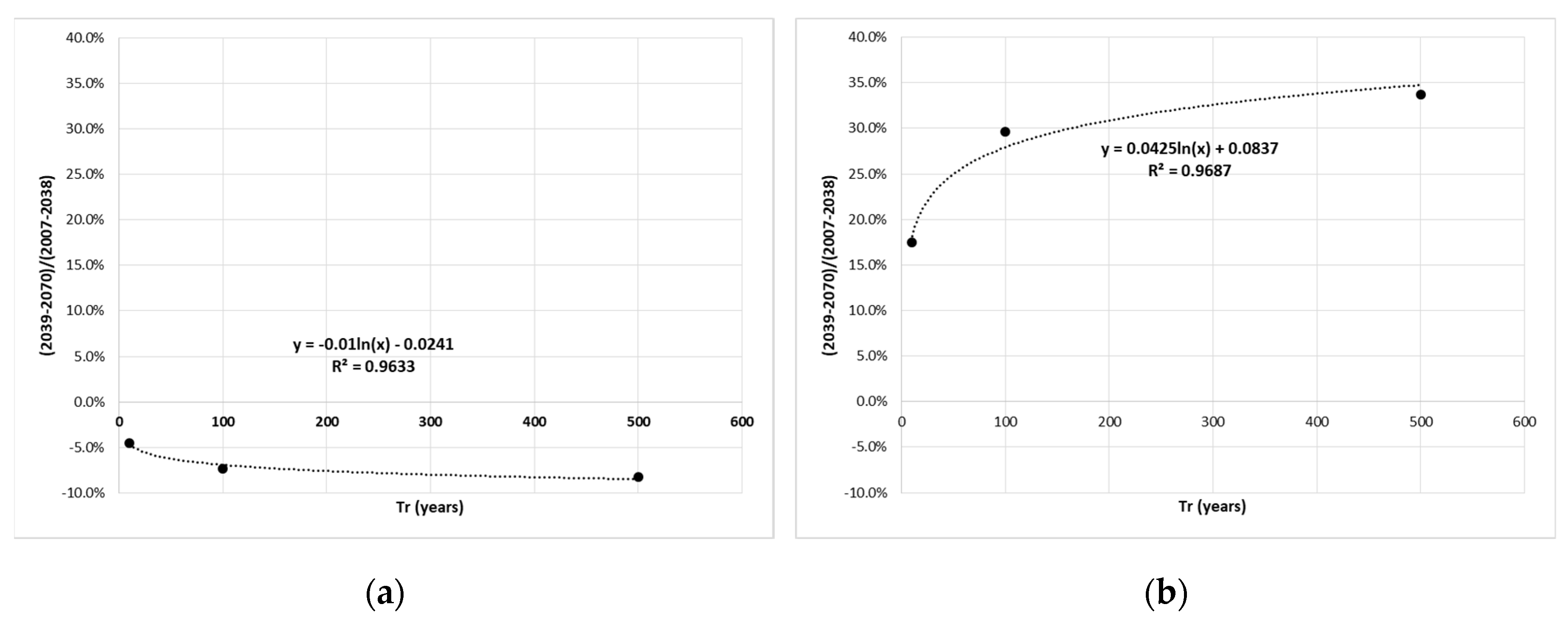
As for flow rate, the MRI-CGCM3 climate model shows an increase in flood risk effects due to climate change, while BCC-CSM1-1-m shows a decrease. Results are enlarged for economic value and inhabitants potentially affected, while flooded surface decreases.
A logarithmic trend line is the one that best fits, and represents how the atmosphere behaves that shows in Figure 12, Figure 13 and Figure 14.
Flooded surface, inhabitants potentially affected and flood economic damage value can be calculated in absolute terms and are shown in Table 4 for ES091_HIJ_01_02_04_05_06.
4. Discussion
4.1. Climate Change Effect
Comparison between observed meteorological data and projections of climate scenarios, for a common time interval, has revealed a significant difference between the series. This means that the results must in any case be interpreted in relative terms, evaluating trends and not absolute values.
Results for both selected climate models show important differences between each other in absolute and relative terms, indicating that there is significant uncertainty in the projections, especially due to rainfall; and they suggest that for local impact studies, further analysis to regionalize outputs from global climate models still needs to be done. For the results to be reliable, climate models must adequately represent extreme phenomena, as most of them are suitable for evaluating water resource evolution.
There is a large uncertainty in climate projections that influences the estimation of future flood risk. The crucial action in the case of adaptation to floods is to carry out a detailed analysis to choose the best climate model and use results in relative terms between the short term (1st Stage) and long term (2nd Stage) of the projection period [4].
The proposed methodology allows one to determine in terms of hazard and flood risk, the effect that climate change has on a given territory, considering both variable rainfall and temperature, and enables a fast evaluation of various climate models and a comparison of their differences.
This evaluation enables one to define actions in terms of a cost–benefit analysis and prioritize the ones that should be included in flood risk management plans due to climate change, as these management plans must contain effective actions in the short, medium and long term and cannot ignore the effect of climate change.
In the specific case of Híjar River Basin, and Reinosa, MRI-CGCM3 model trend analysis shows that climate change will increase damage to society, both economic and personal, while BCC-CSM1-1-m shows a small decrease. As the MRI-CGCM3 model fits better with annual maximum real daily flow rates than BCC-CSM1-1-m, it can be concluded that climate change will cause a significant increase of potential affected inhabitants and economic damage due to flood risk that will require mitigation actions.
This assumption might match with previous years’ observations, especially given the high number of low probability events recorded in Spain. This is the specific case of the Hijar River that in 2019 registered two floods, the one on December 2019 being the largest ever registered in Reinosa Gauging Station and related with a low probability event (300 years return period). This conclusion is consistent with the Fifth Assessment Report (AR5) of the IPCC (2013–14), which points out that it is likely that the frequency or intensity of intense rainfall has increased in Europe.
4.2. Future Research
As already mentioned, this methodology could be applied in every potential significant flood risk area through a water authority flood risk management plan in order to prioritize actions.
Firstly, all available regional climate models could be selected and evaluated. Finally, a sensitive RCP analysis with RCP 4.5 scenario could be carried out.
Supplementary Materials
The following are available online at https://www.mdpi.com/2073-4441/12/4/1114/s1. Spreadsheet1: Climate_Models_Input_Data.xlsm.
Author Contributions
Conceptualization, E.L. and G.C..; methodology, E.L. and G.C.; project administration, G.C.; software, E.L.; validation, G.C.; formal analysis, E.L.; writing—original draft preparation, E.L.; writing—review and editing, E.L. and G.C.; visualization, F.J.T.; supervision, F.J.T. All authors have read and agreed to the published version of the manuscript.
Funding
This research received no external funding.
Acknowledgments
The authors acknowledge ASTER model developer J. A. Collado (SPESA Ingenieria); F. J. Sanchez and M. Aparicio (Spanish Ministry for Ecological Transition and the Demographic Challenge); M. L. Moreno and L. Polanco (Ebro Water Authority); and the Ebro Water Authority.
Conflicts of Interest
The authors declare no conflict of interest.
References
- EEA. Mapping the Impacts of Natural Hazards and Technological Accidents in Europe; EA Technical Report No 13/2010; European Environment Agency: Copenhagen, Denmark, 2010; Available online: http://www.eea.europa.eu/publications/mapping-the-impacts-of-natural (accessed on 10 January 2020).
- Planes de Gestión del Riesgo de Inundación. Ministerio para la Transición Ecológica y el Reto Demográfico. Available online: https://www.miteco.gob.es/es/agua/temas/gestion-de-los-riesgos-de-inundacion/planes-gestion-riesgos-inundacion/ (accessed on 15 December 2019).
- Yuanyuan, L.; Sayers, P.; Yuanyuan, L.; Galloway, G.; Penning-Rowsell, E.; Fuxin, S.; Kang, W.; Yiwei, C.; Quesne, T.L.; Asian Development Bank; et al. Flood Risk Management: A Strategic Approach. Available online: https://unesdoc.unesco.org/ark:/48223/pf0000220870 (accessed on 16 January 2020).
- Doroszkiewicz, J.; Romanowicz, R.J.; Kiczko, A. The Influence of Flow Projection Errors on Flood Hazard Estimates in Future Climate Conditions. Water 2019, 11, 49. [Google Scholar] [CrossRef] [Green Version]
- Zhu, T.; Lund, J.R.; Jenkins, M.W.; Marques, G.F.; Ritzema, R.S. Climate change, urbanization, and optimal long-term floodplain protection. Water Resour. Res. 2007, 43, 122–127. [Google Scholar] [CrossRef] [Green Version]
- Nyaupane, N.; Thakur, B.; Kalra, A.; Ahmad, S. Evaluating Future Flood Scenarios Using CMIP5 Climate Projections. Water 2018, 10, 1866. [Google Scholar] [CrossRef] [Green Version]
- Intergovernmental Panel on Climate Change. Available online: https://archive.ipcc.ch/ (accessed on 20 December 2019).
- European Flood Awareness System (EFAS). Available online: https://www.efas.eu/en/news/summary-efas-notifications-2019 (accessed on 3 January 2020).
- European Commission. Directive 2007/60/Ec of the European Parliament and of the Council of 23 October 2007 on the assessment and management of flood risks. Off. J. L 288/27 2007, 8, 27–34. [Google Scholar]
- Garijo, C.; Mediero, L. Influence of climate change on flood magnitude and seasonality in the Arga River catchment in Spain. Acta Geophys. 2018, 66, 769–790. [Google Scholar] [CrossRef]
- Garijo, C.; Mediero, L.; Garrote, L. Usefulness of AEMET generated climate projections for climate change impact studies on floods at national-scale (Spain). Ingeniería del Agua 2018, 22, 153–166. [Google Scholar] [CrossRef] [Green Version]
- Cantarino, I. Modelo *Aster. Fundamentos y Aplicación; Ministerio de Medio Ambiente: Madrid, Spain, 1998.
- Cobos, G.; Collado, J.A. ASTER. Modelo Hidrológico De Simulación Y Previsión Aplicado A Cuencas Donde El Fenómeno Nival Es Relevante. Manual De Usuario. Available online: http://www.spesa.es/paginas/basededatos/ASTER_Manual_Usuario.pdf (accessed on 27 December 2019).
- Jiménez, A.; Montañés, C.; Mediero, L.; Incio, L.; Garrote, J. El Mapa De Caudales Máximos De Las Cuencas Intercomunitarias. Revista De Obras Públicas 2012, 3533, 7–32. Available online: https://www.miteco.gob.es/es/agua/temas/gestion-de-los-riesgos-de-inundacion/snczi/Mapa-de-caudales-maximos/ (accessed on 28 December 2019).
- Propuesta de mínimos para la realización de los mapas de riesgo de inundación. Directiva de inundaciones – 2° ciclo; Ministerio para la Transición Ecológica: Madrid, Spain, 2019. Available online: https://www.miteco.gob.es/en/agua/temas/gestion-de-los-riesgos-de-inundacion/Metodologia%20mapas%20de%20riesgo%20Dir%20Inundaciones%20JULIO%202013_tcm38-98530.pdf (accessed on 29 December 2019).
- Policy-Relevant Assessment of Socio-Economic Effects of Droughts and Floods, To Establish a Damage-Water Depth Relationship. Available online: http://www.feem-project.net/preempt/ (accessed on 29 December 2019).
- Cobos, G. Cuantificación De Las Reservas Hídricas En Forma De Nieve Y Previsión En Tiempo Real De Los Caudales Fluyentes De La Fusión. Aplicación Al Pirineo Español: Cuenca Alta Del Río Aragón. Ph.D. Thesis, Universitat Politècnica de València, Valencia, Spain, 2004. [Google Scholar]
- Cobos, G.; Frances, M.; Arenillas. The ERHIN Programme. Hydrological-Nival Modelling for the Management of Water Resources in the Ebro Basin. La Houille Blanche 2010, 3, 58–64. [Google Scholar] [CrossRef]
- Anderson, E.A. Development and Testing of Snow Pack Energy Balance Equations. Water Resour. Res. 1968, 4, 19–37. [Google Scholar]
- Anderson, E.A. National Weather Service River Forecast System. Snow Accumulation and Ablation Model; US Department of Commerce, National Oceanic and Atmospheric Administration, National Weather Service: Silver Spring, MA, USA, 1973.
- Anderson, E.A. A Point Energy and Mass Balance Model of a Snow Cover; US Department of Commerce, National Oceanic and Atmospheric Administration, National Weather Service, Office of Hydrology: Silver Spring, MA, USA, 1976.
- Anderson, E.A. Snow Accumulation and Ablation Model—SNOW 17; US Department of Commerce, National Oceanic and Atmospheric Administration, National Weather Service, National Weather Service River Forecast System: Newburyport, MA, USA, 2006; p. 61.
Figure 1.
Reinosa (Cantabria, Spain). 20th December 2019.

Figure 2.
Hijar river basin. (a) Overall Site map. (b) Detailed Site map.

Figure 3.
Hijar potential significant flood risk (ES091_HIJ_01_02_04_05_06). http://iber.chebro.es/SitEbro/sitebro.aspx.
Figure 3.
Hijar potential significant flood risk (ES091_HIJ_01_02_04_05_06). http://iber.chebro.es/SitEbro/sitebro.aspx.

Figure 4.
Overall methodology scheme.

Figure 5.
(a) Flood surface, (b) inhabitants potentially affected and (c) economic damage value in terms of flow rate in A203 gauging station.
Figure 5.
(a) Flood surface, (b) inhabitants potentially affected and (c) economic damage value in terms of flow rate in A203 gauging station.

Figure 6.
ASTER hydrological model. Hijar river basin mesh (grey grid), Gauging Station (A203), rainfall stations (9008E, 9012) and temperature stations (2225, 2232).
Figure 6.
ASTER hydrological model. Hijar river basin mesh (grey grid), Gauging Station (A203), rainfall stations (9008E, 9012) and temperature stations (2225, 2232).

Figure 7.
ASTER hydrological model snow accumulation (snow–water equivalent) (a) Day 1, (b) Day 2. Hijar model (ranging from 1 mm–pink to 215 mm–cyan).
Figure 7.
ASTER hydrological model snow accumulation (snow–water equivalent) (a) Day 1, (b) Day 2. Hijar model (ranging from 1 mm–pink to 215 mm–cyan).

Figure 8.
Upper level. Real (blue) and calculated (red) daily flow rates in A203. Lower level. Snow water equivalent in the catchment for the calibration period.
Figure 8.
Upper level. Real (blue) and calculated (red) daily flow rates in A203. Lower level. Snow water equivalent in the catchment for the calibration period.

Figure 9.
Upper level. Real (blue) and calculated (red) daily flow rates in A203. Lower level. Snow water equivalent in the catchment for the validation period.
Figure 9.
Upper level. Real (blue) and calculated (red) daily flow rates in A203. Lower level. Snow water equivalent in the catchment for the validation period.

Figure 10.
Daily flow rate evolution during control period (1961–2000) for real data (blue), BCC (green) and MRI (red). (a) Annual maximum, (b) annual mean.
Figure 10.
Daily flow rate evolution during control period (1961–2000) for real data (blue), BCC (green) and MRI (red). (a) Annual maximum, (b) annual mean.

Figure 11.
Flow rate projection ratio (2nd Stage (2039–2070)/1st Stage (2007–2038)) trend line in terms of return periods. (a) Analog method (ANA)—BCC-CSM1-1-m; (b) ANA—MRI-CGCM3.
Figure 11.
Flow rate projection ratio (2nd Stage (2039–2070)/1st Stage (2007–2038)) trend line in terms of return periods. (a) Analog method (ANA)—BCC-CSM1-1-m; (b) ANA—MRI-CGCM3.

Figure 12.
Second Stage (2039–2070)/1st Stage (2007–2038) flood surface ratio trend line in terms of return periods. (a) ANA—BCC-CSM1-1-m; (b) ANA—MRI-CGCM3.
Figure 12.
Second Stage (2039–2070)/1st Stage (2007–2038) flood surface ratio trend line in terms of return periods. (a) ANA—BCC-CSM1-1-m; (b) ANA—MRI-CGCM3.

Figure 13.
Second Stage (2039–2070)/1st Stage (2007–2038) economic damage ratio trend line in terms of return periods. (a) ANA—BCC-CSM1-1-m; (b) ANA—MRI-CGCM3.
Figure 13.
Second Stage (2039–2070)/1st Stage (2007–2038) economic damage ratio trend line in terms of return periods. (a) ANA—BCC-CSM1-1-m; (b) ANA—MRI-CGCM3.

Figure 14.
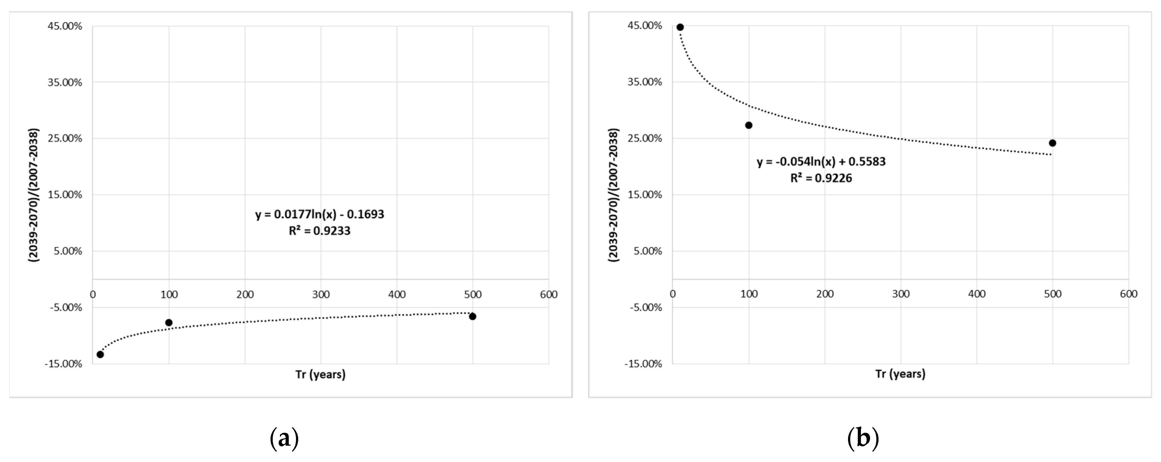
Second Stage (2039–2070)/1st Stage (2007–2038) inhabitants potentially affected ratio trend line in terms of return periods. (a) ANA—BCC-CSM1-1-m; (b) ANA—MRI-CGCM3.
Figure 14.
Second Stage (2039–2070)/1st Stage (2007–2038) inhabitants potentially affected ratio trend line in terms of return periods. (a) ANA—BCC-CSM1-1-m; (b) ANA—MRI-CGCM3.


Table 1.
Instant (15 minute) flow rate, flood surface, inhabitants potentially affected and economic damage 1.
Table 1.
Instant (15 minute) flow rate, flood surface, inhabitants potentially affected and economic damage 1.
| Instant Flow Rate (m3/s) | Return Period (years) | Surface (km2) | Inhabitants | Economic Value (€) |
|---|---|---|---|---|
| 138 | 10 | 2.783 | 346 | 29,194,901 |
| 214 | 100 | 3.843 | 982 | 56,806,383 |
| 273 | 500 | 4.620 | 1484 | 90,791,074 |
1 Obtained for overall ES091_HIJ_01_02_04_05_06 potential significant flood risk area, including the Spanish Public Water Domain (RDPH).
Table 2.
Return period, daily flow rate projection, 1st Stage (2007–2038); daily flow rate projection ratio, 2nd Stage (2039–2070); and flow rate ratio (2nd Stage/1st Stage).
Table 2.
Return period, daily flow rate projection, 1st Stage (2007–2038); daily flow rate projection ratio, 2nd Stage (2039–2070); and flow rate ratio (2nd Stage/1st Stage).
| ANA—BCC-CSM1-1-m | |||
| Tr (years) | Flow Rate Projection 2007–2038 (m3/s) | Flow Rate Projection 2039–2070 (m3/s) | 2039–2070/ 2007–2038 1 (%) |
| 10 | 28.13 | 27.00 | 96.0% |
| 25 | 31.92 | 30.62 | 95.9% |
| 50 | 34.73 | 33.30 | 95.9% |
| 100 | 37.52 | 35.96 | 95.9% |
| 500 | 43.96 | 42.11 | 95.8% |
| ANA—MRI-CGCM3 | |||
| Tr (years) | Flow Rate Projection 2007–2038 (m3/s) | Flow Rate Projection 2039–2070 (m3/s) | 2039–2070/ 2007–2038 1 (%) |
| 10 | 27.36 | 31.05 | 113.5% |
| 25 | 31.99 | 36.51 | 114.1% |
| 50 | 35.43 | 40.57 | 114.5% |
| 100 | 38.85 | 44.59 | 114.8% |
1 Column 3 divided by column 2.
Table 3.
Projection ratio 2nd Stage (2039–2070)/1st Stage (2007–2038) for the flow rate, flood surface, inhabitants potentially affected and flood damage’s economic value.
Table 3.
Projection ratio 2nd Stage (2039–2070)/1st Stage (2007–2038) for the flow rate, flood surface, inhabitants potentially affected and flood damage’s economic value.
| ANA—BCC-CSM1-1-m | |||||
| Flow Rate (%) | Instant Flow Rate (m3/s) | Return Period (years) | Flood Surface (%) | Inhabitants (%) | Economic Value (%) |
| −4.0 | 132.4 | 10 | −2.9 | −13.3 | −4.5 |
| −4.1 | 205.1 | 100 | −3.1 | −7.6 | −7.3 |
| −4.2 | 261.5 | 500 | −3.2 | −6.6 | −8.2 |
| ANA—MRI-CGCM3 | |||||
| Flow Rate (%) | Instant Flow Rate (m3/s) | Return Period (years) | Flood Surface (%) | Inhabitants (%) | Economic Value (%) |
| 13.5 | 156.7 | 10 | 9.6 | 44.8 | 17.4 |
| 14.8 | 245.6 | 100 | 11.0 | 27.3 | 29.7 |
| 15.3 | 314.7 | 500 | 11.4 | 24.2 | 33.7 |
Table 4.
Absolute terms for the flow rate, flood surface, inhabitants potentially affected and flood damage’s economic value for selected climate change projections 1.
Table 4.
Absolute terms for the flow rate, flood surface, inhabitants potentially affected and flood damage’s economic value for selected climate change projections 1.
| ANA—BCC-CSM1-1-m | ||||
| Flow Rate (m3/s) | Return Period (years) | Surface (km2) | Inhabitants | Economic Value (€) |
| 132.4 | 10 | 2.703 | 300 | 27,887,407 |
| 205.1 | 100 | 3.722 | 907 | 52,640,944 |
| 261.5 | 500 | 4.472 | 1386 | 83,327,840 |
| ANA—MRI-CGCM3 | ||||
| Flow Rate (m3/s) | Return Period (years) | Surface (km2) | Inhabitants | Economic Value (€) |
| 156.7 | 10 | 3.049 | 501 | 34,286,399 |
| 245.6 | 100 | 4.263 | 1250 | 73,649,691 |
| 314.7 | 500 | 5.145 | 1843 | 121,426,897 |
1 Obtained for overall ES091_HIJ_01_02_04_05_06 potential significant flood risk area, including the Spanish Public Water Domain (RDPH).
© 2020 by the authors. Licensee MDPI, Basel, Switzerland. This article is an open access article distributed under the terms and conditions of the Creative Commons Attribution (CC BY) license (http://creativecommons.org/licenses/by/4.0/).
Share and Cite
MDPI and ACS Style
Lastrada, E.; Cobos, G.; Torrijo, F.J. Analysis of Climate Change’s Effect on Flood Risk. Case Study of Reinosa in the Ebro River Basin. Water 2020, 12, 1114. https://doi.org/10.3390/w12041114
AMA Style
Lastrada E, Cobos G, Torrijo FJ. Analysis of Climate Change’s Effect on Flood Risk. Case Study of Reinosa in the Ebro River Basin. Water. 2020; 12(4):1114. https://doi.org/10.3390/w12041114
Chicago/Turabian StyleLastrada, Eduardo, Guillermo Cobos, and Francisco Javier Torrijo. 2020. "Analysis of Climate Change’s Effect on Flood Risk. Case Study of Reinosa in the Ebro River Basin" Water 12, no. 4: 1114. https://doi.org/10.3390/w12041114
Note that from the first issue of 2016, this journal uses article numbers instead of page numbers. See further details here.