Intertwining Observations and Predictions in Vadose Zone Hydrology: A Review of Selected Studies

Abstract

Observing state variables, fluxes, and key properties in terrestrial ecosystems should not be seen as disjointed, but rather as fruitfully complementary to ecosystem dynamics modeling. This intertwined view should also take the organization of the monitoring equipment into due account. This review paper explores the value of the interplay between observations and predictions by presenting and discussing some selected studies dealing with vadose zone hydrology. I argue for an advanced vision in carrying out these two tasks to tackle the issues of ecosystem services and general environmental challenges more effectively. There is a recognized need to set up networks of critical zone observatories in which strategies are developed and tested that combine different measurement techniques with the use of models of different complexity.

1. Introduction

Intertwining the description of observed variables and system parameters with model simulations is definitely not new in science. However, on the one hand, it is not always clear how this integration should take place and, on the other, especially in the past, in most cases the measurements concerned were not performed by those who actually developed and/or used the model. The latter situation has generated interesting discussions about the lack of communication and collaboration between these two worlds, but sometimes has also triggered the most heated debates during conferences or even within research project meetings [1,2].

Fortunately, in the present time, most of the causes that have hampered the dialog between experimentalists and modelers are collapsing in succession. Reticence and reluctance to exchange information, the fact that the rapid advance in modeling tools did not go hand in hand with the development of new or more precise measurement techniques, are concerns that are now being at least mitigated or even eliminated by the following two key factors: (i) that the very structure of funded research projects facilitates and strengthens greater levels of science-sharing, and (ii) the setting-up and management of critical zone observatories (CZOs) require improvements in collecting and sharing big data as well as further cooperation among scientists who have different experience and expertise.

The United Nations’ 15-year plan of action “2030 Agenda for Sustainable Development” [3] should be viewed as inextricably linked to the concepts of ecosystem functions and services [4]. These two blueprints, among other things, are the driving factors behind carrying out ever more integrated research into, for example, the water–food–energy–ecosystem nexus [5], and the increasing establishment of long-term environmental monitoring infrastructures in different parts of the world, albeit concentrated in the United States and Europe [6]. Consequently, we are witnessing a boom in the monitoring and modeling of water flow and solute transport in the soil–vegetation–atmosphere system and toward the groundwater. This all involves a number of research activities, such as the development of networks of wireless sensors and cosmic-ray neutron probes, ecohydrological studies on stable isotopes of hydrogen and oxygen specifically applied to elucidate plant transpiration, improvements in mapping soil properties and environmental variables for model parameterization by coupling random forest techniques with geostatistics, and the continuous upgrade of computer models by using ever more efficient numerical algorithms or implementing additional modules that account for new monitoring techniques.

Most of the observed and modeled processes in the vadose zone occur mainly in the one-dimensional, vertical direction [7]. Therefore, for the sake of effectiveness of this review article, one can suitably refer to the nonlinear, parabolic differential equation that governs the isothermal water flow in a variably saturated rigid soil, while neglecting the role of air phase on the liquid flow process, that is, the following well-known, pressure-based 1-D Richards equation (RE):

$$C\left(h\right)\frac{\partial h\left(z,t\right)}{\partial t}=\frac{\partial }{\partial z}\left\{K\left[\theta \left(h\right)\right]\left[\frac{\partial h\left(z,t\right)}{\partial z}-1\right]\right\}-{\mathsf{\Sigma }}_w\left(h\right)$$

(1)

where t is time, z is a vertical coordinate (taken positive downward), h is matric suction head (i.e., the absolute value of matric pressure head, with dimension of L and commonly with units of cm), C(h) = dθ/dh is the soil water capacity function (which can be readily obtained from the knowledge of the soil water retention function, θ(h), as will be described in the next section), and θ is the volumetric soil water content (with the dimension of L³L⁻³ and commonly with units of cm³ cm⁻³). Together with the soil water retention function, the other soil hydraulic characteristic in Equation (1) is the hydraulic conductivity function, K[θ(h)] (K has the dimension of LT⁻¹ and commonly the units of cm h⁻¹). Following a macroscopic approach for root uptake, the extraction function, Σ_w(h) (sink term), depends on the water potential at the plant crown and is computed by allowing for osmotic potential and both the resistances to water flow in the rhizosphere and within the roots [8]. The Richards equation (RE) offers a comprehensive description of water flow movement in the soil–vegetation–atmosphere continuum, but may become rather unmanageable for applications at relatively large spatial scale, not because of computational issues, but rather as a result of the spatial, and sometimes also temporal, variability exhibited by the soil hydraulic properties and some boundary conditions (especially the conditions at the lower boundary of the flow domain).

To overcome some difficulties and drawbacks of the RE, the daily soil–moisture dynamics can be described by resorting to an integral, but simplified, description of the hydrological processes occurring on a vegetated land surface known in the literature as the bucketing approach. In most cases, this model assumes the soil as being made up of a single layer that behaves like a bucket, receiving and retaining all incident water until its storage capacity is filled. One very popular single-layer bucket model (BM) has the following mathematical form [9,10]:

$$n Z_r \frac{dS\left(t\right)}{dt}=\pi \left[S\left(t\right), t\right]-\chi \left[S\left(t\right)\right],$$

(2)

where the right-hand side of Equation (2) comprises the following incoming (π) and outgoing fluxes (χ):

$$\pi \left[S\left(t\right), t\right]=P\left(t\right)-CI\left(t\right)-Q\left[S\left(t\right),t\right],$$

(3a)

$$\chi \left[S\left(t\right)\right]=E\left[S\left(t\right)\right]+T\left[S\left(t\right)\right]+L\left[S\left(t\right)\right]$$

(3b)

Equation (2) describes the soil moisture balance for a uniform soil layer of depth Z_r, with average soil porosity por, and average degree of soil saturation S (0 ≤ S ≤ 1) (at the Darcy scale, equal to θ/por) over the entire rooting zone. Note that a more functional than physical meaning should be attached to soil depth Z_r as it should be associated more effectively to the hydrologically active, uniform soil control volume where the evapotranspiration process plays a dominant role. In Equations (3a) and (3b), P is the precipitation rate; CI is the canopy interception rate; Q is the surface runoff rate; E and T are actual evaporation and transpiration rates, respectively; and L is the leakage rate (i.e., the drainage losses) from the lower boundary of the soil profile. When using Equation (2), the time dimension commonly has units of “day” and flux has units of “mm day⁻¹”. This form of BM is a stochastic linear ordinary differential equation because the term P has a stochastic nature [11].

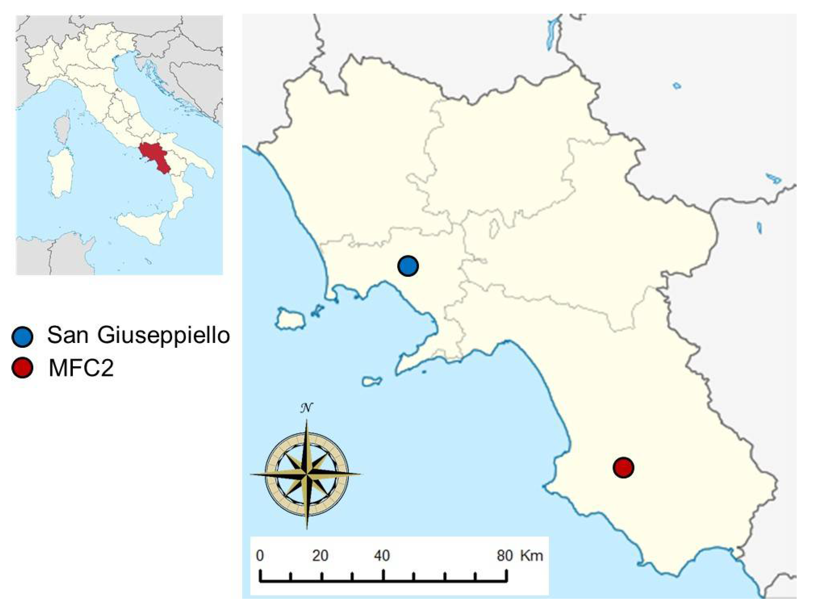
After a brief introduction to the dynamics of the hydrological processes taking place in the groundwater–soil–vegetation–atmosphere system, the remainder of this review proceeds with issues concerning the determination of soil hydraulic characteristics that are key input parameters of hydrological models. Subsequently, tools for measuring and detecting the space-time variability of soil moisture are discussed as this variable is one of the most important state variables of hydrological processes. Finally, and by merging the previous sections in some way, both monitoring and modeling issues are addressed in combination by using the research activities currently underway in the Alento critical zone observatory (CZO). The discussion on the results from these selected investigations winds its way through both the whole Campania (southern Italy; see Figure 1) and some field sites in this region. The map of an indicator of soil hydrological response concerns the entire administrative area of Campania, whereas the analysis and mapping of field-scale soil moisture variability using different techniques refer to two distinct sites: the San Giuseppiello and Monteforte Cilento (MFC2) experimental sites. San Giuseppiello is a contaminated area situated in the municipality of Giugliano (Naples, Italy; see the blue dot in Figure 1) that was confiscated by the authorities from a criminal organization and used to run phytoremediation experiments with poplars and evaluate the feasibility of using groundwater contaminated by volatile organic compounds for irrigation purposes only. MFC2 is located near the village of Monteforte Cilento (Salerno, Italy; see the red dot in Figure 1) and is one of the two test sub-catchments that was selected because it is more representative of the agroforestry ecosystems of the Alento CZO.

2. Observation of Soil Properties: Measurements of Soil Hydraulic Characteristics and Their Variability

Assessing the soil hydrological response using either the Richards-based or bucket-based hydrological models requires knowledge of the nonlinear relationships between the soil water suction head, h; the volumetric soil water content, θ; and the hydraulic conductivity, K. Although these relationships are quite complex and can also exhibit a hysteretic behavior, especially in the case of coarser-textured soils, they are commonly synthesized by the soil water retention, θ(h), and hydraulic conductivity, K[θ(h)], functions. These two functions are referred to as the soil hydraulic properties and are key parameters featuring of the Richards Equation (1), or are required to correctly estimate soil parameters of the bucket model (Equation (2)).

2.1. Basic Soil Hydraulic Characteristics Featuring in the Richards Equation

For mathematical convenience and efficiency when solving the Richards equation, soil hydraulic properties are described by analytical parametric relationships. A commonly used parametric expression for the soil water retention function (WRF) is that of van Genuchten [12]:

$$\mathsf{\Theta }\left(h\right)=\frac{\theta \left(h\right)-{\theta }_r}{{\theta }_s-{\theta }_r}={\left[1+{\left(\alpha \times h\right)}^n\right]}^{-m},$$

(4)

which has proved successful thanks to the fact that its parameters can be employed to estimate the relative hydraulic conductivity (K_r) function (HCF) only by providing a value for the saturated hydraulic conductivity, K_s, as follows:

$$K_r\left(\mathsf{\Theta }\right)=\frac{K\left(S_e\right)}{K_s}={\mathsf{\Theta }}^{\lambda }{\left[1-{\left(1-{\mathsf{\Theta }}^{\frac{1}{m}}\right)}^m\right]}^2.$$

(5)

In Equations (4) and (5), θ_s and θ_r are the saturated and residual volumetric soil water contents, respectively; α (cm⁻¹) is a scale parameter; and n (-) and m = (1–1/n) are shape parameters of WRF. Parameter λ (-) is the pore connectivity/tortuosity parameter of HCF, usually assumed as a coefficient set at 0.5 or −1.0. Effective soil saturation, Θ, varies between 0 (when θ = θ_r) and 1 (when θ = θ_s). These two parametric expressions are known in the literature as the unimodal van Genuchten–Mualem (vGM) soil hydraulic relations. However, Romano and Santini [13] suggested that in some cases, such as for finer-textured soils, more reliable parameter estimates can be obtained by decoupling the two soil hydraulic functions and, for example, one can use the van Genuchten water retention relation and the Brooks and Corey hydraulic conductivity relation (see [12] for the latter relationship).

To overcome some drawbacks of unimodal hydraulic relationships, such as vGM relations, Priesack and Durner [14] described soil hydraulic properties with closed-form multi-modal relations of the van Genuchten–Mualem type. Instead, Romano et al. [15] developed bimodal lognormal relationships as soil hydraulic properties with the following key features: they too are closed-form parametric expressions, but have a sound theoretical basis and enable a more general conceptualization of soil to be provided.

Whatever the unimodal, bimodal, or multi-modal soil hydraulic relationships that one would like to employ, the relevant unknown parameters are determined through direct or indirect methods to be performed in the laboratory or in situ [16,17,18]. Without going into the description of a multitude of laboratory methods, it is suffice to mention here that only the evaporation experiment whose measured data can be used either in a direct manner or with an inverse modeling technique. According to this test, a soil sample is first saturated from below and then dried by evaporation from the upper boundary and with the lower end completely sealed. During this test, the total sample weight and matric suction heads at several soil depths are measured. Romano and Santini [13] employed these measured data to simultaneously estimate the unknown soil hydraulic parameters using an inverse method. Through both experimental and numerical evaluations of the inverse method, they also showed that the length of the soil sample and the number of matric suction sensors can be conveniently reduced to make the evaporation test faster without losing too much in terms of accuracy and precision. The values measured during an evaporation test can instead be also employed within a direct method. To the author’s knowledge, Gardner and Miklich [19] were the first to come forward with the idea of determining soil hydraulic properties by using evaporation data in a sort of instantaneous profile procedure that was then pursued by Wind [20]. This direct technique has been continuously improved and is still receiving additional contributions (e.g., [21,22,23].

The plots in Figure 2 depict the soil hydraulic properties of a soil core collected in the uppermost soil horizon of the MFC2 experimental site located in the Upper Alento River Catchment (UARC) [24]. This soil core was subjected to an evaporation experiment in the laboratory to obtain the water retention (see Figure 2a) and unsaturated hydraulic conductivity (see Figure 2b) data-points using the Wind method as refined by Iden and Durner [22]. Additional soil water retention data points were measured in the dry range with a pressure plate apparatus. All the measured water retention data points are shown in Figure 2a, and were fitted to either the unimodal (vG-WRF, dashed line) or bimodal (bVG-WRF, solid line) van Genuchten water retention relations. The saturated soil water content, θ_s, was measured in the laboratory and was equal to 0.463 cm³ cm⁻³, whereas the residual soil water content, θ_r, was set at zero. By measuring the saturated hydraulic conductivity value, K_s, in the laboratory by the falling-head method (K_s = 0.955 cm h⁻¹) and setting the tortuosity parameter λ = −1, Figure 2b depicts either the unimodal (dashed line) or bimodal (solid line) van Genuchten hydraulic conductivity relations as predicted using either the unimodal or bimodal water retention parameters. From a perusal of the solid and dashed curves shown in these two plots, it is evident that if one fails to model the actual hydraulic behavior of this soil core correctly, at least by a bimodal hydraulic functions, there may be dramatic consequences on the prediction of the unsaturated hydraulic conductivity characteristic, hence on the fluxes simulated by a water budget model. This outcome further corroborates the findings of Priesack and Durner [14], Romano et al. [15], and Romano and Nasta [25].

Determination in situ of the soil hydraulic properties can be obtained, among other techniques, by running a field drainage test whose measured data can again be exploited within either direct or inverse methods. Running a field test has the undoubted advantage of efficiently accounting for the presence of different layers in the soil profile, this being a rule rather than an exception in the real world. An interesting development of this field experiment was achieved by Vachaud et al. [26], whereas Dane and Hruska [27] used the field drainage data within an inversion procedure. As was done for the laboratory evaporation experiment by Romano and Santini [13], for the field drainage experiment Romano [28] provided useful insights for optimally designing this test, especially to make the experimental procedures somewhat simpler without excessively increasing the level of uncertainty in parameter estimation. Among other things, Romano [28] evaluated the feasibility to include the lower boundary condition as an additional unknown parameter to be determined because this position allows for the overcoming of the limitation of setting the lower boundary condition in an actual soil profile.

Actually, an inverse problem can be defined as the calculation of the cause given the effect and expressed as follows [29]:

$$v_{obs}=\partial O\left({\xi }_{obs};p;b;s\right)+\epsilon$$

(6)

where v_obs is a set of observed variables, ∂O represents a generic partial differential operator (the model, for short), ξ_obs is the vector of a space/time coordinate in which v_obs is observed, p is the vector of the model parameter, b is a set of initial/boundary conditions, s is a control variable (e.g., sinks or sources), and ε is the error in both model and measured quantities. Therefore, model calibration can be formulated as (i) the inverse problem of identifying model parameter, p; (ii) the inverse problem of estimating the initial condition, b; or (iii) the inverse problem of locating a point source, s. When p, b, and s are known, Equation (6) is the so-called direct (or forward) problem (usually ε is set at zero in this case), whereas some information on ε is required when formulating the inverse problem. Most of the studies dealing with soil hydrology refer to the inverse problem of parameter identification and specifically with the estimation of the soil hydraulic parameters [30].

2.2. Basic Soil Hydraulic Characteristics Featuring in the Bucket Model

A lumped macroscale soil water budget framed within the bucketing approach is mainly controlled by the following key soil hydraulic parameters: the soil water contents at field capacity, θ_FC, and permanent wilting, θ_WP. These two hydraulic parameters characterize the soil water capacity of the bucket in the rooting zone. Some authors would rather refer to these hydraulic parameters as the upper and lower limits of the water contents of the soil reservoir, respectively [31,32].

In almost all cases, the permanent wilting point (θ_WP) is derived from the soil water retention function (see Equation (4)) when the matric suction head takes on the value h_PW = 150 m, which is considered a sort of standard measure of this soil condition [8]. This definition was derived from the observed soil matric suction head when a dwarf sunflower (Helianthus annuus L.), which was employed as an indicator plant, wilted permanently while failing to recover its turgor upon rewetting. Referring to this wilting point has the distinct advantage that the soil water content value can be easily measured in the laboratory using a pressure plate apparatus. This is clearly a simplified definition because the permanent wilting point actually depends not only on the type of plant (e.g., h_PW values increase when moving from hydrophytes to xerophytes), but also on local environmental conditions because the atmospheric water demand can achieve such a high rate that a plant may wilt, even if a relatively good amount of soil water is present in its rhizosphere.

The “field capacity” in a uniform soil profile is also a rather ill-defined soil water condition in the rhizosphere, and the related value of water content in the soil becomes a parameter subjected to slightly different meanings and determination methods. In a very simplified view, the value of θ_FC is roughly determined from the soil water retention function at the matric suction head of 3.30 m, mostly for medium-textured soils. However, it has been widely shown that more appropriate values for θ_FC are estimated by assuming h_FC = 1.00 m in the case of coarser-textured soils and h_FC = 5.00 m in the case of finer-textured soils [8,33].

The above-mentioned criticisms of the conditions of “field capacity” and “permanent wilting” in a soil profile call for a different perspective to parameterize a bucket-type hydrological model more efficiently. Romano and Santini [8] pointed out that θ_FC is a process-dependent parameter related to a specifically designed drainage experiment to be carried out in situ, especially to account for soil layering because layered soil profiles are the rule rather than exception in actual field conditions. As also discussed by Twarakavi et al. [34], Nasta and Romano [35] showed that the soil water content value at “field capacity” can be conveniently estimated through a synthetic drainage process, and proposed, on a closer examination of the problem, that the flux-based “field capacity” criterion is also a sound technique to identify “effective” soil hydraulic parameters of a layered soil profile to be then conveniently used in a single-layer bucket model.

Therefore, especially allowing for the present-day availability of soil data and computer tools, a modern and more effective way to determine the water capacity of a soil reservoir is to resort to the output of a comprehensive hydrological model. Instead of using the difference θ_FC-θ_WP as a “static” indicator of the available soil water for plant growth (plant-available soil water, PAW), Romano and Santini [8] were perhaps the first to suggest that a “dynamic” (or functional) indicator for PAW should be identified by running a soil–vegetation–atmosphere (SVA) model to compute the variable τ_S that represents the maximum rate at which a rooting system of the plant can uptake water from the soil profile in the absence of water stress. Unlike the static indicator, the use of this dynamic indicator has highlighted how and to what extent the determination of PAW is affected not only by the textural characteristics of soil (as can be retrieved only by calculating the “static” difference θ_FC-θ_WP), but also and more importantly by the type of vegetation and the atmospheric conditions of the local climate.

2.3. Simplified Estimation of the Soil Hydraulic Characteristics and Their Variability

Laboratory or field tests to determine the soil water retention, θ(h), and hydraulic conductivity, K[θ(h)], functions are notoriously burdensome and time-consuming; hence, their use hampers the important issue of retrieving information about the spatial, and sometimes also the temporal, variations exhibited by these characteristics over a certain area. A popular way to overcome this difficulty is to resort to pedotransfer functions (PTFs) that enable the parameters describing the soil hydraulic properties to be estimated from soil properties that are measured with relatively ease and more cost-effectively, such as particle-size distribution, soil organic carbon content, oven-dry bulk density, soil pH, and free calcium carbonate [36].

Nowadays the term PTF has a much wider meaning than in the past and, generally speaking, refers to a way of obtaining difficult-to-retrieve model parameters by transferring knowledge on more easily measurable properties. The downside of a PTF is that it should be considered as strictly valid only within the local area where it was developed because many studies have demonstrated that the accuracy and precision of a PTF can decrease even significantly when it is applied in another environment (e.g., [37]). Instead of developing a new PTF for predicting the soil water retention functions in a certain area, Romano and Palladino [38] put forward the idea that an already established PTF can be locally calibrated by using specific terrain attributes and showed that this procedure can at least reduce the prediction bias within a reasonable value for practical applications. Locally calibrated PTFs are then fruitfully exploited to also obtain information on the structure of spatial variability exhibited by the soil hydraulic properties [39,40]. However, considerable research efforts would be needed to develop efficient PTFs for unsaturated hydraulic conductivity functions. Because recent PTFs are now able to estimate relatively well the scale, α, and shape, n, parameters featuring van Genuchten’s WRF, it has been recognized that a research challenge would be to reduce the uncertainty in estimating parameter K_s as much as possible. Interesting approaches to the latter issue are reported in some recent papers [41,42,43].

As shown by Pringle et al. [40], point estimates offered by a PTF are usually affected by relatively large errors and the main application of such a simplified method is therefore to predict unknown parameters in an efficient and especially cost-effective way over a not-too-small modeling grid. For the benefit of a wider readership, it is useful to close this sub-section by briefly mentioning another issue that comes into play when applying a PTF to map a regionalized variable—interpolation can be done either before or after applying a PTF to predict the target variable, a problem that seems somewhat overlooked or even omitted in a few studies. Therefore, the “interpolate first, then predict (IF-tP)” technique, where the available soil properties are first interpolated to obtain a map of input data for the PTF over the study area, might be in contrast to the “predict first, then interpolate (PF-tI)” alternative because the models governing vadose zone hydrology are highly nonlinear [44]. The above-mentioned techniques can thus generate different maps and even a complete mismatch in some specific cases. Even if neither technique was found to be superior to the other, the IF-tP technique, which first interpolates the measured basic soil properties (i.e., the input for the PTF) and then applies the selected PTF to the interpolated data for estimating the target variable, seems to provide better outcomes than the other way round (e.g., [45,46]).

Within the strategic plan “Transparency in Campania”, which was designed to characterize the main environmental compartments in the region of Campania (southern Italy), more than 3300 locations were visited (see Figure 3a) to collect disturbed and undisturbed topsoil samples to determine soil physical, chemical, and hydraulic properties. The collected datasets were exploited to map different soil quality indicators in the entire region using a random forest kriging technique [47]. As an example, Figure 3b shows the spatial distribution in Campania of the “plant available soil water”, namely, θ_FC-θ_WP, by assuming the soil as uniform in each location and estimating both these variables by using pedotransfer functions found in the literature.

3. Observation of Key State Variables: Soil Moisture Measurements and Space-Time Variations

Soil moisture is an important hydrologic state variable and commonly defined as the volume of water that is present in a certain volume of a field soil [48]. Detection of the soil volume involved in the dynamics of vadose zone processes depends on the type of problem to be tackled [49], but is also influenced by the measuring technique employed to determine the soil moisture values. Sensor devices placed on spaceborne platforms (e.g., the Sentinel family) or unmanned aerial systems (UASs) enable the volumetric soil moisture contents to be observed only in the uppermost soil layer of a certain area (usually the top 5 cm of the soil profile). This information is very valuable for computing evapotranspiration fluxes at the land surface. When dealing with the onset of vegetation stress or rainfall-triggered landslides, one should determine the spatial and temporal fluctuations of soil moisture in the entire rooting zone, or even below it, and ground-based sensor techniques help tackle these problems more effectively. The present-day complex issues of irrigation water management or groundwater recharge require soil moisture monitoring by using an integrated array of ground- and satellite-based sensors, together with recently developed proximal sensing that includes UASs or stationary and rover cosmic-ray neutron probes (CRNPs) (e.g., [50]).

Therefore, the above-mentioned soil volume should be viewed in more “functional” than “physical” terms, and has almost nothing to do with the well-known concept of “representative elementary volume” (REV), which is mainly associated with the definition of intrinsic soil physical properties, such as soil porosity. Measurements of the water present in a very small volume of soil, say at a point scale, can be done using the gamma-ray technique [48]. The thermo-gravimetric technique, which is the only available direct method and therefore considered a point of reference for comparisons, in practice measures the water contained in a soil volume not less than about 200 cm³, hence at a local scale because it entails the collection of an undisturbed soil core of appropriate size depending mostly on its soil texture [51]. A widely used and quite accurate method to measure water in the soil at the local scale under both laboratory and field conditions is time domain reflectometry (TDR), which is an indirect method that measures the bulk soil dielectric permittivity and infers, through a calibration relationship, the water content in a soil volume whose size is a function of the length of the rods and their configuration. Even the recently-developed capacitance sensors have a spatial resolution and sensitivity to soil moisture that depends on the specific configuration of the probe. An indirect method that still operates at the local scale, but is now almost completely abandoned, is based on neutron thermalization that, however, deduces soil moisture values in a volume that mainly depends on the degree of soil saturation (specifically, it is a sphere with a diameter of about 20 cm for larger soil wetness or an ellipsoid with the longest diameter even as much as 60–70 cm in the case of dry soil). Electrical resistivity tomography (ERT) has become another very popular method to monitor soil moisture dynamics [52].

A review of the available methods to measure soil moisture lies far beyond the scope of this article, but it can be useful to briefly present the monitoring program set-up by Palladino et al. [53] at the San Giuseppiello experimental site to explore the feasibility of using groundwater contaminated by volatile organic compounds (VOCs) for irrigation purposes only. This site was planted with poplar trees (Populus nigra spp.) for field-scale demonstrations of phytoremediation activities conducted on some contaminated agricultural areas surrounding the metropolitan city of Naples (Italy). We designed this program by coupling the monitoring of soil water status (with capacitance and porous sensors) and plant responses (using dendrometers) with two geophysical techniques comprising both 2D and 3D cross-hole ERT and Mise-a-la-Masse (MALM) techniques. ERT is a well-known geophysical method, as is MALM, but recently the latter technique has yielded valuable results in elucidating the interactions between soil and vegetation [54]. In this investigation, MALM is complementary to ERT in providing further insights into poplar responses so that water flow and solute transport models are run more effectively.

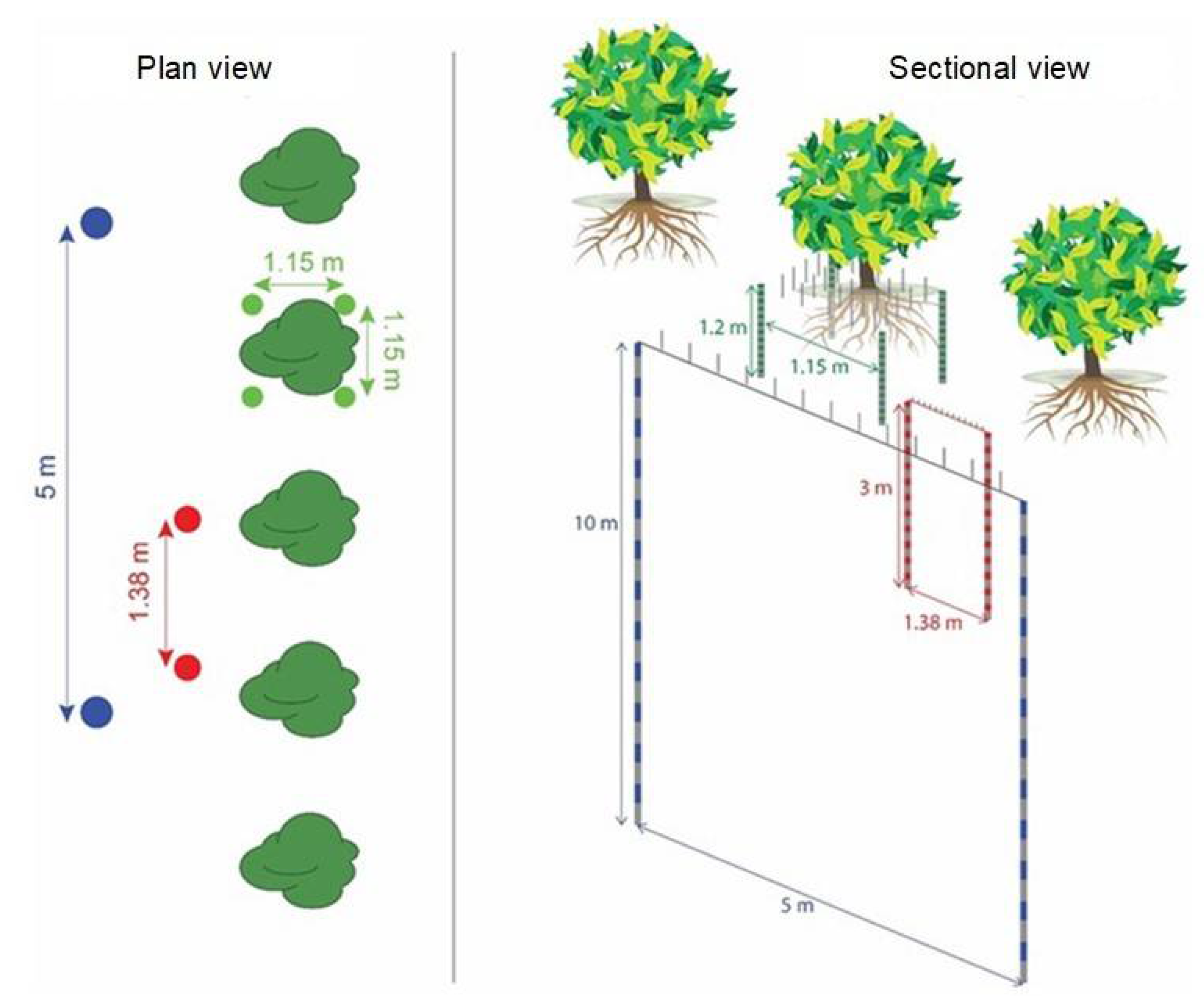
The schematic in Figure 4 shows the ERT monitoring system that consists of three cross-well sub-systems with different locations (see the plan view), reaching different soil depths (see the sectional view). These sub-systems can be briefly described as follows:

• A 3D sub-system consisting of four near-surface boreholes (each 1.2 m in length) drilled at the corners of a square (each side measuring 1.15 m) centered on one of the poplars. Each of these boreholes contains 12 stainless steel electrodes, 0.10 m apart. This monitoring sub-system is complemented by 24 stainless steel electrodes inserted in the soil surface to form an equally spaced grid around the trunk of the poplar. In sum, this subsystem comprises 72 electrodes;
• A 2D subsystem consisting of two 3-m-long boreholes, spaced 1.38 m apart, each containing 24 stainless steel electrodes, with a vertical spacing of 0.12 m. Between these two boreholes, 13 equally spaced stainless steel electrodes were also inserted at the soil surface, making a total of 61 electrodes;
• A 2D subsystem consisting of two 10-m-long boreholes, spaced 5.0 m apart, each containing 24 stainless steel electrodes, with a vertical spacing of 0.4 m. Between these two boreholes, 13 equally-spaced stainless steel electrodes were also inserted at the soil surface for a total of 61 electrodes.

The soil at San Giuseppiello is a typical Andosol of the Campania plain originating from the eruptions of Mt. Somma-Vesuvius. A soil survey made in a pedological pit dug close to the ERT measurements have revealed the following average soil physical characteristics:

• at soil depths of 5–20 cm, soil texture is 42.23% sand, 45.82% silt, and 11.95% clay, whereas the oven-dry bulk density is 1.074 g/cm³;
• at soil depths of 50–75 cm, soil texture is 47.45% sand, 39.73% silt, and 12.82% clay, whereas the oven-dry bulk density is 0.993 g/cm³;
• at soil depths of 110–125 cm, soil texture is 42.55% sand, 49.69% silt, and 7.76% clay, whereas the oven-dry bulk density is 1.080 g/cm³;
• at soil depths of 162–177 cm, soil texture is 39.90% sand, 52.34% silt, and 7.76% clay, whereas the oven-dry bulk density is 1.062 g/cm³.

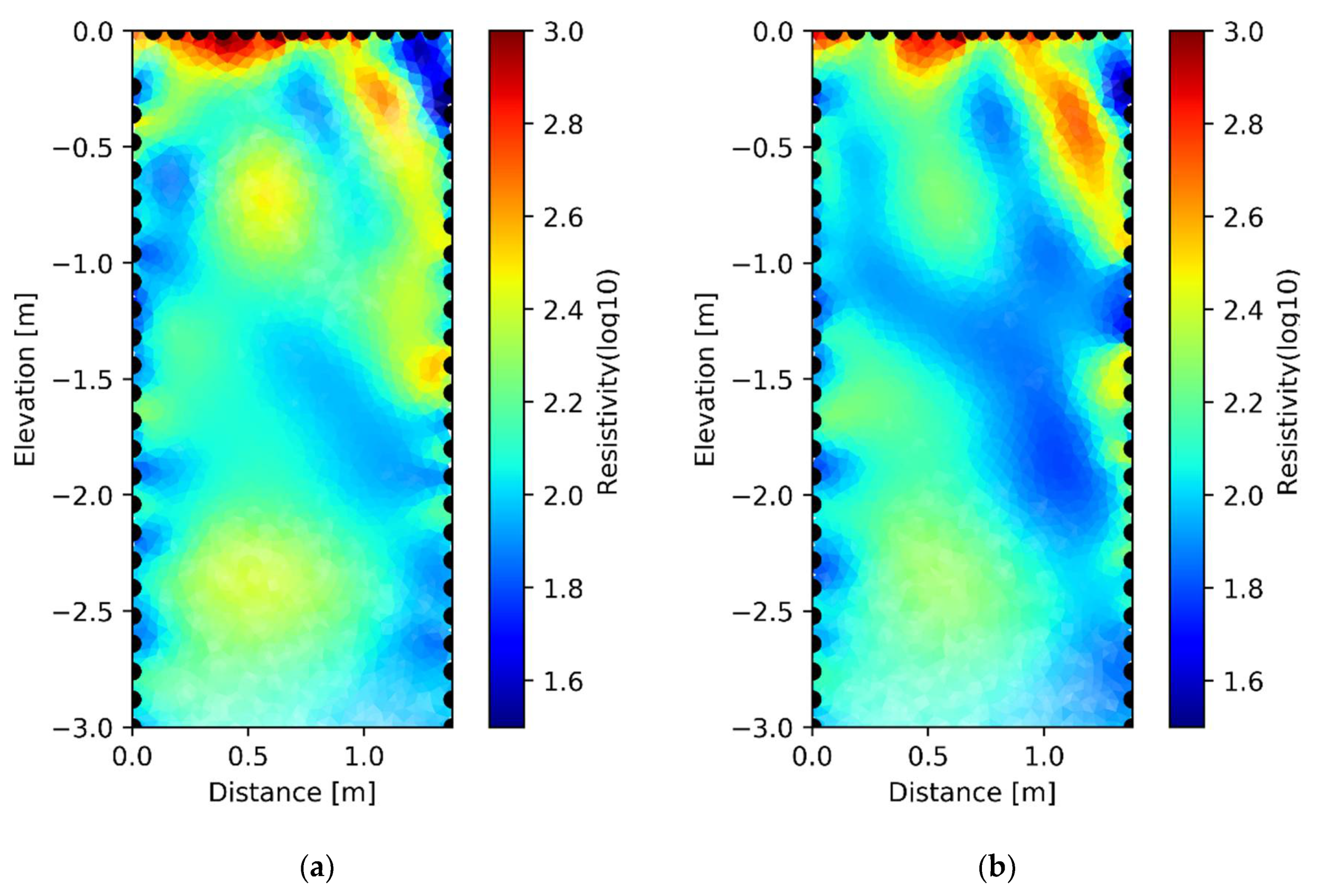
The panels of Figure 5 show the results of the 2D geophysical time-lapse monitoring carried out in October 2019 at the beginning (on 22 October 2019; see Figure 5a) and after the end (on 25 October 2019; see Figure 5b) of an irrigation event. It should first be noted that although the soil physical properties varied little along the vertical profile, both electrical resistivity panels of this figure instead revealed the presence of some sort of heterogeneity. However, in the uppermost soil layer, up to approximately 1.0 m, the observed variations in log₁₀ electrical resistivity did not depend on natural soil variability, but should rather be mainly attributed to the presence of the typical radial and vertical distribution of the roots of the poplar trees. Overall, the most resistive region (more reddish colors) was located near the soil surface and especially in close proximity to the poplar tree. Another resistive soil layer was located approximately in a zone of the profile centered around a soil depth of about 2.5 m. On the left upper side of the 22 Oct 2019 panel (see Figure 5a), the presence of very low resistivity levels due to the infiltrating water at the beginning of the irrigation event was also quite evident. The 2D resistivity image relative to the end of the irrigation event (see the right panel of Figure 5) depicts the significant changes in log₁₀ resistivity because of the soil water redistribution, drainage, and evapotranspiration processes after about 3 days of water supply.

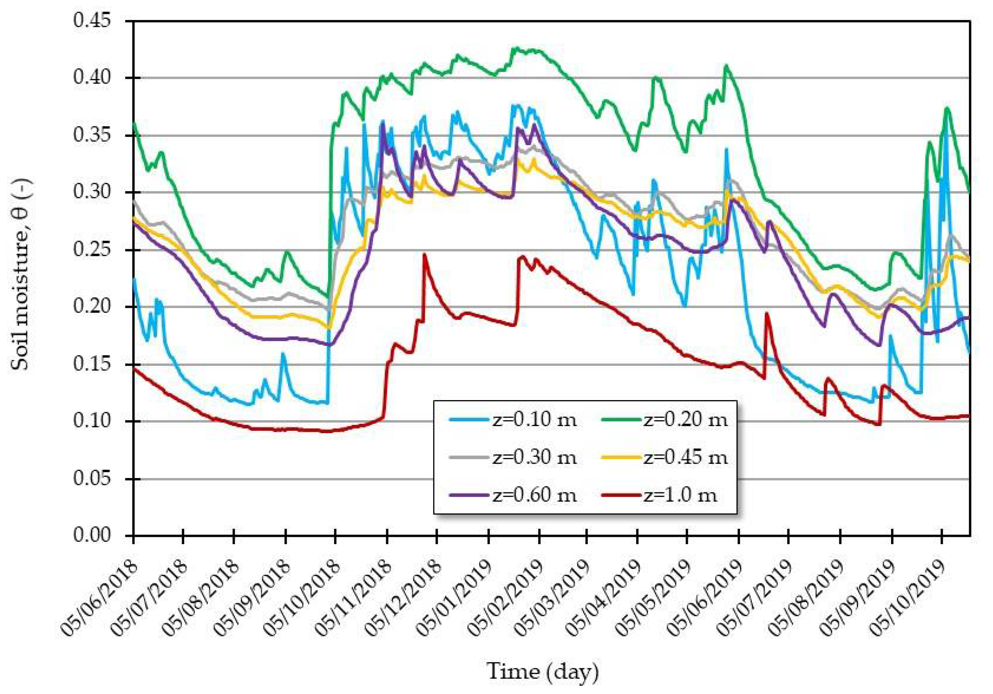
This geophysical monitoring system was coupled, also for calibration/validation purposes, to a system for continuous monitoring of soil water status in the rooting zone of the poplars. This system comprised the following sensors installed in a pit: six Greenhouse Sensors GS3 (METER Group, Inc., USA) capacitance probes, for simultaneous measurements of soil moisture, soil temperature, and apparent electrical conductivity at the soil depths of 0.10, 0.20, 0.30, 0.45, 0.60, and 1.0 m; four Matric Potential Sensors MPS-6 (METER Group, Inc., USA) porous probes that measure matric pressure potentials at the soil depths of 0.20, 0.30, 0.45, and 0.60 m. Note that the GS3 and MPS-6 probes positioned at the same soil depth provided data-points of the soil water retention functions at the relevant soil depths of the pit. Moreover, the gradients between the matric pressure sensors gave an indication about the water fluxes in the vertical direction. As an example of the data collected by this additional monitoring system, Figure 6 shows the dynamics of soil moisture at different soil depths over about one and a half years of operation. This graph clearly shows that the deepest soil layer (i.e., at 1.0 m depth) remained at the driest conditions almost throughout the monitored period, whereas the time variations of soil moisture were more erratic in the upper soil layer (i.e., in the first 0.30 m of soil thickness) as the typical consequence of the dynamics of the infiltration and evapotranspiration processes.

Another example of integration between different soil moisture monitoring techniques can be found in the recent study by Nasta et al. [55]. This kind of integration is definitely not new in the literature, but the cited investigation brought some elements of novelty regarding the refinement of the calibration procedures of the Sentinel-1 Synthetic Aperture Radar (SAR) images to obtain more reliable near-surface soil moisture maps in a small catchment subject to typical Mediterranean rainfall seasonality. Ground-truthing enabling the remotely sensed soil moisture to be validated was provided not only by capacitance probes inserted at different soil depths in 20 locations of the study site, but also by one stationary cosmic-ray neutron probe positioned in the center of the monitoring grid.

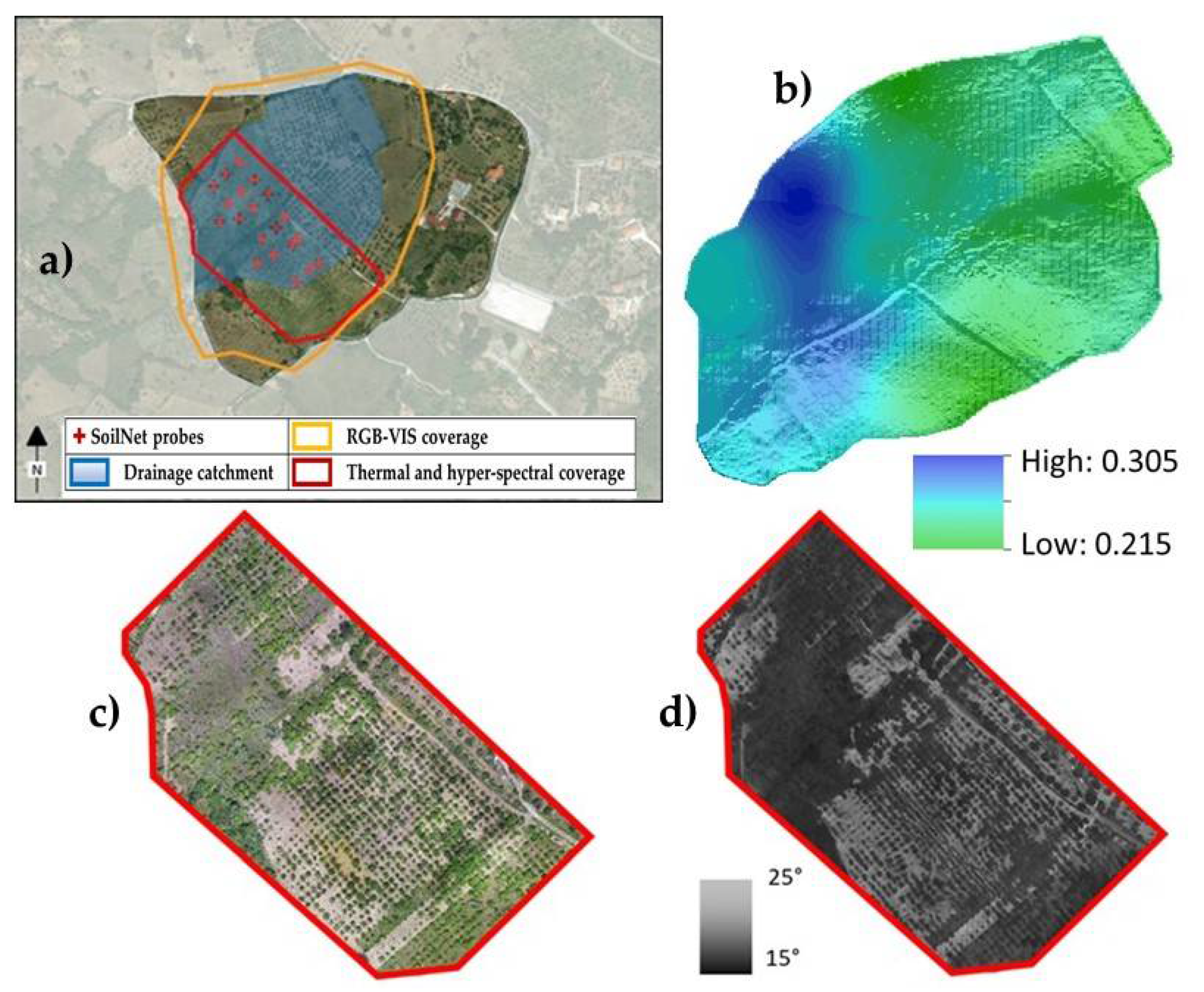
A fruitful merging of different measuring techniques can be found in the field activities specifically devoted to monitoring near-surface soil moisture underway in the MFC2 site (see the red dot in Figure 1), one of the two test sub-catchments established in the Upper Alento River Catchment (UARC; [24]). Within the European Cooperation in Science and Technology (COST) “Harmonious” project [56], a specific field campaign was designed and carried out in this experimental site to explore the potential offered by UASs to obtain hyper-resolution mapping based on visible, hyperspectral, and thermal imagery for retrieving the spatial distribution of soil moisture (see Figure 7). The UAS is based on an octocopter that covered a roughly rectangular area, with a size approximately 400 × 200 m² (see Figure 7a). The flight ran simultaneously with the measurement of near-surface soil moisture values using TDR probes of 15 cm in length and inserted vertically into the soil, and the relevant soil moisture map is depicted in Figure 7b. The set of UAS data were assembled to obtain RGB and thermal ortho-mosaic imageries (see plots Figure 7c,d).

4. Integrating Observations and Modeling Activities: The Case of the Alento CZO

In the previous sections, a few studies were presented that employed different measuring technologies to address some specific research questions. In this section, instead, the important role exerted by the interplay between observations and predictions is discussed with an overview of the activities underway in the Alento critical zone observatory (CZO) established to serve as a representative area of the Mediterranean region.

The Alento River Catchment (ARC) was in the past the setting only of some sparse investigations dealing with geological studies, mainly aiming to characterize the typical flysch of the Cilento area (province of Salerno), as well as rainfall-runoff modeling for flood frequency estimation. More systematic investigations started in the late 1980s when public bodies, together with local farmers’ unions and stakeholders, developed a plan to improve the local socio-economic conditions of the area that had become very depressed mainly because of land abandonment after World War II. Given that the area in question has a strong farming tradition and provides the inspiration for the United Nations Educational, Scientific and Cultural Organization (UNESCO) heritage-listed Mediterranean diet (thanks to Ancel Keys after his visit to the Cilento area), a system of artificial water reservoirs was constructed primarily for irrigation purposes. The main component of this system is the Piano della Rocca earthen dam, which has operated since 1995, and releases water for irrigation, drinking, and hydroelectric uses. This dam subdivides, from both the physical and functional viewpoints, the entire ARC into the Upper Alento River Catchment (UARC), with a drainage area of 102 km², and the Lower Alento River Catchment (LARC), with a drainage area of 309 km². In the last two decades, integrated studies have been undertaken in the area, especially in the UARC, and the reader wishing additional details is directed to the paper by Romano et al. [24]. Investigations in the UARC are being carried out at different spatial scales: the scale of the entire upper catchment (102 km²) and the scale of experimental sub-catchments (each about 10 to 20 hectares) that are used as being representative of the main landscape characteristics of UARC.

Modeling activity at the spatial scale of the entire UARC was mainly carried out using the Soil and Water Assessment Tool (SWAT) package [57]. To obtain soil water balance simulations, which are as reliable as possible, this model was fed with a large quantity of good-quality weather, terrain, land-use/land-cover, and soil property information retrieved from intensive field campaigns and both laboratory and in situ tests [58,59,60]. By exploiting this bulk of input information to parameterize the SWAT model, Nasta et al. [57] investigated the effects exerted on forest–water interactions by the observed land abandonment in UARC, a situation that started in the early 1960s and that has since been experienced by many depressed rural areas in the Mediterranean region. In what way and to what extent afforestation or deforestation affects water resources in catchments is still a controversial matter and a subject of lively debate among scientists who espouse the demand-side or supply-side views of the matter [61]. The scale issue certainly plays a key role here. Without a focus on the latter point, one is most likely to have difficulty highlighting which process may be dominant, thus failing to provide adequate support for decision-making. A response to the question might be sought by enlarging the spatial area of interest to be able to better account for land-atmosphere feedback and precipitation recycling.

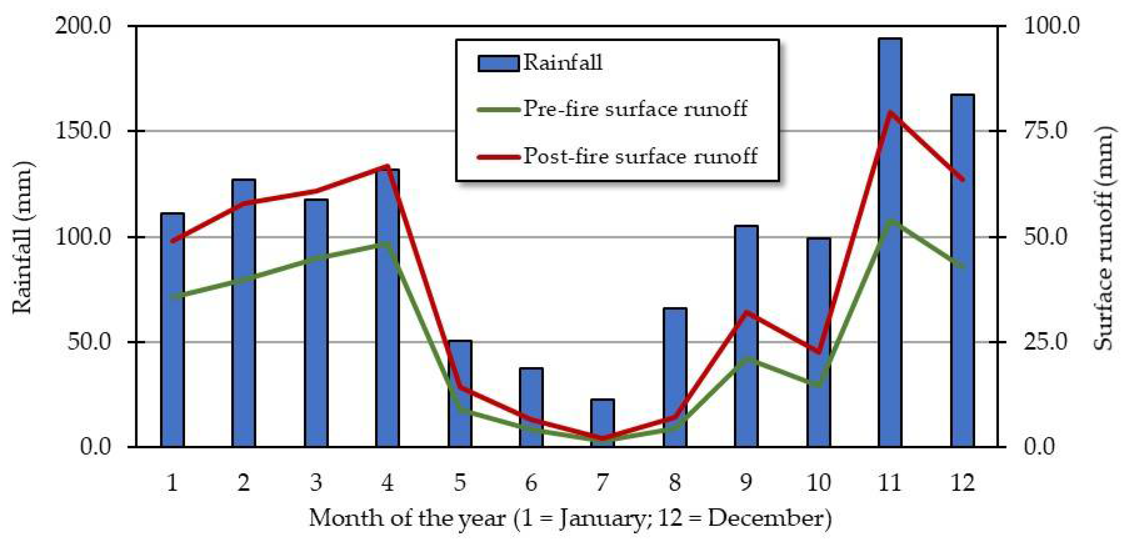
Shifting to a problem that is related to the presence of forested areas in a catchment and their potential as burning biomass (e.g., see [62]), researchers carried out an analysis in the UARC to predict the consequences of wildfires. This is an issue of great concern, partly because the UARC belongs to the Cilento, Vallo di Diano, and Alburni National Park, the largest national park in Italy (covering a protected area of 178,172 hectares). After model calibration and testing using the streamflow data recorded at the Piano della Rocca earthen dam, SWAT was run throughout a simulation period of 5 (pre-fire) plus 5 (post-fire) years, that is, initially under a no-fire scenario and then for a 5-year post-fire scenario obtained by changing the model parameters that govern the land uses, vegetation interception, and soil infiltration as a function of burn severity. Figure 8 reports the mean monthly rainfall (in mm) over the simulation periods and shows the comparison between the pre-fire (green line) and post-fire (red line) mean monthly surface runoff (in mm). Precipitation being equal, the patterns of these lines not only confirmed a somewhat obvious outcome, that is, that an increase in runoff occurred under the post-fire condition, but also highlight the dramatic consequences that the typical seasonality of the Mediterranean climate can cause. The intense rainfall events that occur after a late summer wildfire (generally toward the end of summer and beginning of autumn) can generate such large runoff volumes as to trigger floods and infrastructure failure.

Moving from the catchment scale to the field scale, MFC2 is an experimental sub-catchment located close to the village of Monteforte Cilento in UARC, where a comprehensive monitoring and modeling program is running with the main aim of detecting the hydrological response of part of the upper Alento catchment used mainly for agroforestry, which is to be compared with a sub-catchment positioned in the intensely forested area of the same upper catchment. The MFC2 sub-catchment was described by Romano et al. [24]. It is suffice to mention here that in this experimental site, a network of wireless sensors (SoilNet) was deployed to measure soil dielectric permittivity, soil electrical conductivity, soil temperature, as well as soil matric pressure potential at the two soil depths of 0.15 and 0.30 m in 20 locations within an area of approximately 300 × 120 m² (a cherry orchard with sparse trees for wood production alone). A cosmic-ray neutron probe that measures average soil moisture is located at the center of this area.

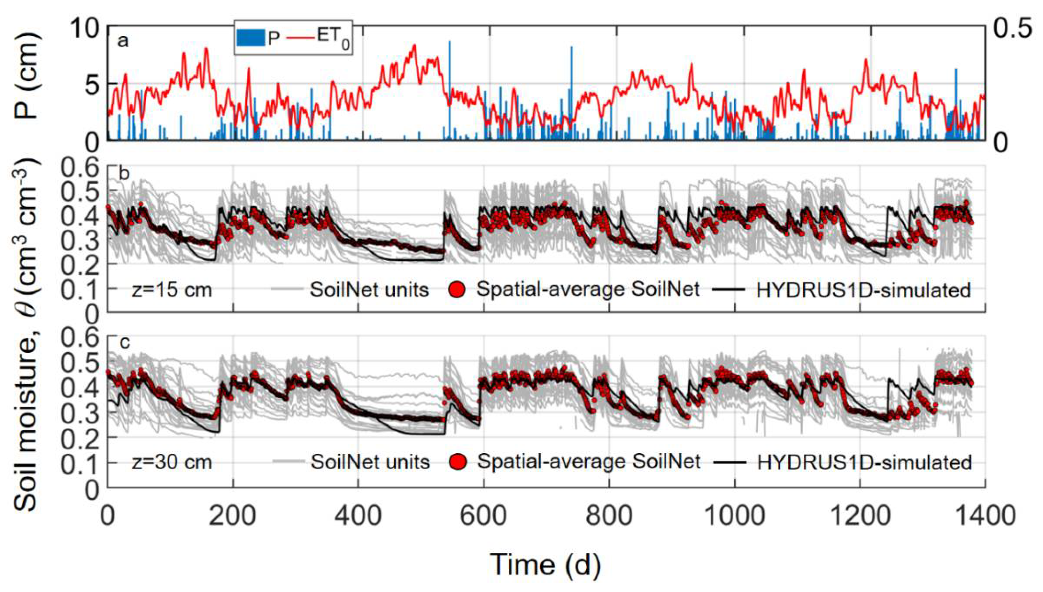
Figure 9 shows the time series of soil moisture contents monitored by the 20 SoilNet end-devices (represented by solid gray lines) at the two soil depths of 0.15 m (panel 9b) and 0.30 m (panel 9c) over a period of 1378 days. As can be seen, the set of gray lines shows some scatter, indicating a somewhat significant spatial variability of soil at the 20 locations, although the soil moisture time series for the soil depth of 0.30 m are contained in a narrower band as might be expected. In both panels, the red circles are the spatial averages of observed soil moisture contents to be compared with the black lines that indicate those predicted using the HYDRUS-1D package [63]. The simulation was run using the average soil hydraulic parameters of a silty clay loam soil, which is the most frequent soil texture in the study site, a 2.0-m-long uniform soil profile with the lower boundary condition set as free drainage, a rooting depth of 0.50 m, and Feddes’ function for plant water stress of a deciduous fruit tree. The initial condition was set as the soil moisture content at “field capacity”, as determined by the numerical procedure suggested by Romano et al. [33].

Although some simplified conditions were adopted to run this numerical simulation, the comparisons between observed and predicted soil moisture contents are very good over most of the monitoring period. During the first 600 days, the greater discrepancies between observed and modeled soil moisture could be seen when the drier periods occurred, with evident underestimates of the model predictions with respect to the observed daily average values. On the other hand, discrepancies were also detected toward the end of the monitoring period when more prolonged rainy days occurred, but in this case the outputs of HYDRUS systematically overpredicted the average observations and this situation was more evident for the data collected at the soil depths of 0.15 m (see panel 9b). Therefore, while feeding the model with these inputs, we were able to predict the average soil moisture dynamics very satisfactorily unless drier or wetter average soil conditions were established in the field. By exploiting the information that we were gathering in the field on the soil hydraulic characteristics at the different soil depths of each location and assigning more accurate initial and lower boundary conditions of the flow domain, we are expecting to gain even better predictions. The upper boundary condition was modeled quite well thanks to the presence of a weather station equipped with precipitation, air temperature, and 4-component net-radiation sensors. To better describe the lower boundary condition, 20 piezometers were installed in June 2020 in this study site to monitor groundwater table.

5. Concluding Remarks and Outlook

Rather than intending to be considered a comprehensive review of monitoring techniques and modeling tools available for investigations in the realm of soil hydrology, this paper surveyed some of the laboratory and field experience gathered by the author’s group with the main aim of discussing the usefulness of fruitfully merging, when possible, information about the characteristics and state of an ecosystem retrieved using different measuring methods. This task is not separate, and should not be viewed as such, from the activity of framing the collected data into models, albeit of different complexity, that enable us not only to describe the observed processes, but principally to interpret them as well as possible to obtain reliable predictions of the complex nonlinear dynamics that govern natural ecosystems.

There is little doubt that present-day progress in sensor technology, the setting-up of new, more accurate measuring techniques; the development of ever more comprehensive computer models; and the fact that much closer mutual cooperation is now required between researchers, authorities, and stakeholders, offer us various opportunities to bridge the gaps still existing between experimentalists and modelers, as well as find suitable and more efficient ways to integrate observations and models over multiple spatial and temporal scales.

References

- Seibert, J.; McDonnell, J.J. On the dialog between experimentalist and modeler in catchment hydrology: Use of soft data for multicriteria model calibration. Water Resour. Res. 2002, 38, 1241. [Google Scholar] [CrossRef]
- Rinderer, M.; Seibert, J. Soil information in hydrologic models: Hard data, soft data, and the dialog between experimentalists and modelers. In Hydropedology—Synergistic Integration of Soil Science and Hydrology; Lin, H., Ed.; Elsevier Academic Press: London, UK, 2012; pp. 515–536. [Google Scholar] [CrossRef]
- United Nations General Assembly. Transforming Our World: The 2030 Agenda for Sustainable Development; A/RES/70/1; United Nations General Assembly: New York, NY, USA, 21 October 2015. [Google Scholar]
- Costanza, R.; d’Arge, R.; de Groot, R.; Farber, S.; Grasso, M.; Hannon, B.; Limburg, K.; Naeem, S.; O’Neill, R.V.; Paruelo, J.; et al. The value of the world’s ecosystem services and natural capital. Nature 1997, 387, 253–260. [Google Scholar] [CrossRef]
- United Nations Economic Commission for Europe. Methodology for Assessing the Water-Food-Energy-Ecosystems Nexus in Transboundary Basins and Experiences from Its Application: Synthesis; United Nations Publication: New York, NY, USA, 2018; pp. 1–66. ISBN 978-92-1-117178-5. [Google Scholar]
- Lin, H.; Hopmans, J.W.; Richter, D.D. Interdisciplinary sciences in a global network of critical zone observatories. Vadose Zone J. 2011, 10, 781–785. [Google Scholar] [CrossRef]
- Vereecken, H.; Huisman, J.A.; Hendricks Franssen, H.J.; Brüggemann, N.; Bogena, H.R.; Kollet, S.; Javaux, M.; van der Kruk, J.; Vanderborght, J. Soil hydrology: Recent methodological advances, challenges, and perspectives. Water Resour. Res. 2015, 51, 2616–2633. [Google Scholar] [CrossRef]
- Romano, N.; Santini, A. Water retention and storage: Field. In Methods of Soil Analysis, Part 4, Physical Methods; SSSA Book Series N. 5; Dane, J.H., Topp, G.C., Eds.; Soil Science Society America: Madison, WI, USA, 2002; pp. 721–738. ISBN 0-89118-841-X. [Google Scholar] [CrossRef]
- Guswa, A.J.; Celia, M.A.; Rodriguez-Iturbe, I. Models of soil moisture dynamics in ecohydrology: A comparative study. Water Resour. Res. 2002, 38, W01166. [Google Scholar] [CrossRef]
- Porporato, A.; D’Odorico, P.; Laio, F.; Ridolfi, L.; Rodriguez-Iturbe, I. Ecohydrology of water-controlled ecosystems. Adv. Water Res. 2002, 25, 1335–1348. [Google Scholar] [CrossRef]
- Rodríguez-Iturbe, I.; Porporato, A. Ecohydrology of Water-Controlled Ecosystems: Soil Moisture and Plant Dynamics; Cambridge University Press: New York, NY, USA, 2005; pp. 1–442. [Google Scholar] [CrossRef]
- Kutilek, M.; Nielsen, D.R. Soil Hydrology; Catena Verlag: Cremlingen-Destedt, Germany, 1994; pp. 1–370. ISBN 3-923381-26-3. [Google Scholar]
- Romano, N.; Santini, A. Determining soil hydraulic functions from evaporation experiments by a parameter estimation Approach: Experimental verifications and numerical studies. Water Resour. Res. 1999, 35, 3343–3359. [Google Scholar] [CrossRef]
- Priesack, E.; Durner, W. Closed–form expression for the multi–modal unsaturated conductivity function. Vadose Zone J. 2006, 5, 121–124. [Google Scholar] [CrossRef]
- Romano, N.; Nasta, P.; Severino, G.; Hopmans, J.W. Using bimodal log-normal functions to describe soil hydraulic properties. Soil Sci. Soc. Am. J. 2011, 75, 468–480. [Google Scholar] [CrossRef]
- Hillel, D.; Krentos, V.D.; Stylianou, Y. Procedure and test of an internal drainage method for measuring soil hydraulic characteristics in situ. Soil Sci. 1972, 114, 395–400. [Google Scholar] [CrossRef]
- Hopmans, J.W.; Šimunek, J.; Romano, N.; Durner, W. Simultaneous determination of water transmission and retention properties: Inverse methods. In Methods of Soil Analysis, Part 4, Physical Methods; SSSA Book Series N. 5; Dane, J.H., Topp, G.C., Eds.; Soil Science Society America: Madison, WI, USA, 2002; pp. 963–1008. ISBN 0-89118-841-X. [Google Scholar] [CrossRef]
- Iovino, M.; Romano, N. Inverse modeling of evaporation and multistep outflow experiments for determining soil hydraulic properties: A comparison. J. Agric. Eng. 2005, 36, 57–67. [Google Scholar]
- Gardner, W.R.; Miklich, F.J. Unsaturated conductivity and diffusivity measurements by a constant flux method. Soil Sci. 1962, 93, 271–274. [Google Scholar] [CrossRef]
- Wind, G.P. Capillary conductivity data estimated by a simple method. In Water in the Unsaturated Zone; Rijtema, P.E., Wassink, H., Eds.; IASAH: Gentbrugge, Belgium, 1968; pp. 181–191. [Google Scholar]
- Peters, A.; Durner, W. Simplified evaporation method for determining soil hydraulic properties. J. Hydrol. 2008, 356, 147–162. [Google Scholar] [CrossRef]
- Iden, S.C.; Durner, W. Free-Form estimation of soil hydraulic properties using Wind’s method. Eur. J. Soil Sci. 2008, 59, 1228–1240. [Google Scholar] [CrossRef]
- Schindler, U.; von Unold, G.; Durner, W.; Müller, L. Evaporation method for measuring unsaturated hydraulic properties of soils: Extending the range. Soil Sci. Soc. Am. J. 2010, 74, 1071–1083. [Google Scholar] [CrossRef]
- Romano, N.; Nasta, P.; Bogena, H.; De Vita, P.; Stellato, L.; Vereecken, H. Monitoring hydrological processes for land and water resources management in a Mediterranean ecosystem: The Alento River catchment observatory. Vadose Zone J. 2018, 17. [Google Scholar] [CrossRef] [Green Version]
- Romano, N.; Nasta, P. How effective is bimodal soil hydraulic characterization? Functional evaluations for predictions of soil water balance. Eur. J. Soil Sci. 2016, 67, 523–535. [Google Scholar] [CrossRef] [Green Version]
- Vachaud, G.; Dancette, C.; Sonko, S.; Thony, J.L. Méthodes de caractérisation hydrodynamique in situ d’un sol non saturé. Application à deux types de sol du Sénégal en veu de la détermination des termes du bilan hydrique. Ann. Agron. 1978, 29, 1–36. [Google Scholar]
- Dane, J.H.; Hruska, S. In-situ determination of soil hydraulic properties during drainage. Soil Sci. Soc. Am. J. 1983, 47, 619–624. [Google Scholar] [CrossRef]
- Romano, N. Use of an inverse method and geostatistics to estimate soil hydraulic conductivity for spatial variability analysis. Geoderma 1993, 60, 169–186. [Google Scholar] [CrossRef]
- Press, W.H.; Teukolsky, S.A.; Vetterling, W.T.; Flannery, B.P. Numerical Recipes in FORTRAN: The Art of Scientific Computing, 2nd ed.; Cambridge University Press: New York, NY, USA, 1992. [Google Scholar]
- Vrugt, J.A.; Bouten, W.; Gupta, H.V.; Hopmans, J.W. Toward improved identifiability of soil hydraulic parameters: On the selection of a suitable parametric model. Vadose Zone J. 2003, 2, 98–113. [Google Scholar] [CrossRef]
- Ritchie, J.T. Soil water availability. Plant Soil 1981, 58, 327–338. [Google Scholar] [CrossRef]
- Logsdon, S. Should upper limit of available water be based on field capacity? Agrosyst. Geosci. Environ. 2019, 2, 190066. [Google Scholar] [CrossRef]
- Romano, N.; Palladino, M.; Chirico, G.B. Parameterization of a bucket model for soil-vegetation-atmosphere modeling under seasonal climatic regimes. Hydrol. Earth Syst. Sci. 2011, 15, 3877–3893. [Google Scholar] [CrossRef] [Green Version]
- Twarakavi, N.K.C.; Sakai, M.; Šimunek, J. An objective analysis of the dynamic nature of field capacity. Water Resour. Res. 2009, 45, W10410. [Google Scholar] [CrossRef]
- Nasta, P.; Romano, N. Use of a flux-based field capacity criterion to identify effective hydraulic parameters of layered soil profiles subjected to synthetic drainage experiments. Water Resour. Res. 2016, 52, 566–584. [Google Scholar] [CrossRef] [Green Version]
- Pachepsky, Y.A.; Rawls, W.J.; Lin, H.S. Hydropedology and pedotransfer functions. Geoderma 2006, 131, 308–316. [Google Scholar] [CrossRef]
- Nasta, P.; Palladino, M.; Sica, B.; Pizzolante, A.; Trifuoggi, M.; Toscanesi, M.; Giarra, A.; D’Auria, J.; Nicodemo, F.; Mazzitelli, C.; et al. Evaluating pedotransfer functions for predicting soil bulk density using hierarchical mapping information in Campania, Italy. Geoderma Reg. 2020, 21, e00267. [Google Scholar] [CrossRef]
- Romano, N.; Palladino, M. Prediction of soil water retention using soil physical data and terrain attributes. J. Hydrol. 2008, 265, 56–75. [Google Scholar] [CrossRef]
- Romano, N. Spatial structure of PTF estimates. In Development of Pedotransfer Functions in Soil Hydrology; Pachepsky, Y.A., Rawls, W.J., Eds.; Elsevier Science BV: Amsterdam, The Netherlands, 2004; pp. 295–319. ISBN 0-444-51705-7. [Google Scholar]
- Pringle, M.J.; Romano, N.; Minasny, B.; Chirico, G.B.; Lark, R.M. Spatial evaluation of pedotransfer functions using wavelet analysis. J. Hydrol. 2007, 333, 182–198. [Google Scholar] [CrossRef]
- Nasta, P.; Vrugt, J.A.; Romano, N. Prediction of the saturated hydraulic conductivity from Brooks and Corey’s water retention parameters. Water Resour. Res. 2013, 49, 2918–2925. [Google Scholar] [CrossRef] [Green Version]
- Pollacco, J.A.; Nasta, P.; Soria-Ugalde, J.M.; Angulo-Jaramillo, R.; Lassabatere, L.; Mohanty, B.P.; Romano, N. Reduction of feasible parameter space of the inverted soil hydraulic parameters sets for Kosugi model. Soil Sci. 2013, 178, 267–280. [Google Scholar] [CrossRef] [Green Version]
- Ghanbarian, B.; Hunt, A.G.; Skaggs, T.H.; Jarvis, N. Upscaling soil saturated hydraulic conductivity from pore throat characteristics. Adv. Water Res. 2017, 104, 105–113. [Google Scholar] [CrossRef] [Green Version]
- Heuvelink, G.B.M.; Pebesma, E.J. Spatial aggregation and soil process modelling. Geoderma 1999, 89, 47–65. [Google Scholar] [CrossRef]
- Sinowski, W.; Scheinost, A.C.; Auerswald, K. Regionalization of soil water retention curves in a highly variable soilscape: II. Comparison of regionalization procedures using a pedotranfer function. Geoderma 1997, 78, 145–160. [Google Scholar] [CrossRef]
- Picciafuoco, T.; Morbidelli, R.; Flammini, A.; Saltalippi, C.; Corradini, C.; Strauss, P.; Blöschl, G. A pedotransfer function for field-scale saturated hydraulic conductivity of a small watershed. Vadose Zone J. 2019, 18. [Google Scholar] [CrossRef] [Green Version]
- Szatmári, G.; Pásztor, L. Comparison of various uncertainty modelling approaches based on geostatistics and machine learning algorithms. Geoderma 2019, 337, 1329–1340. [Google Scholar] [CrossRef]
- Romano, N. Soil moisture at local scale: Measurements and simulations. J. Hydrol. 2014, 516, 6–20. [Google Scholar] [CrossRef]
- Seneviratne, S.I.; Corti, T.; Davin, E.L.; Hirschi, M.; Jaeger, E.B.; Lehner, I.; Orlowsky, B.; Teuling, A.J. Investigating soil moisture-climate interactions in a changing climate: A review. Earth Sci. Rev. 2010, 99, 125–161. [Google Scholar] [CrossRef]
- Babaeian, E.; Sadeghi, M.; Jones, S.B.; Montzka, C.; Vereecken, H.; Tuller, M. Ground, proximal, and satellite remote sensing of soil moisture. Rev. Geophys. 2019, 57, 530–616. [Google Scholar] [CrossRef] [Green Version]
- Topp, G.C.; Ferré, P.A. The soil solution phase: Water Content. In Methods of Soil Analysis, Part 4, Physical Methods; SSSA Book Series N. 5; Dane, J.H., Topp, G.C., Eds.; Soil Science Society America: Madison, WI, USA, 2002; pp. 417–545. ISBN 0-89118-841-X. [Google Scholar] [CrossRef]
- Vereecken, H.; Huisman, J.A.; Bogena, H.R.; Vanderborght, J.; Vrugt, J.A.; Hopmans, J.W. On the value of soil moisture measurements in vadose zone hydrology: A review. Water Resour. Res. 2008, 44, W00D06. [Google Scholar] [CrossRef] [Green Version]
- Palladino, M.; Sica, B.; Chiavarini, S.; Rimauro, J.; Salluzzo, A.; Mary, B.; Boaga, J.; Cassiani, G.; Romano, N. On reducing VOCs concentration from groundwater for irrigation purposes: A detailed monitoring program to test the stripping efficiency of a sprinkler system. In Proceedings of the IEEE International Workshop on Metrology for Agriculture and Forestry (MetroAgriFor), Portici (Naples), Italy, 24–26 October 2019; pp. 286–290. [Google Scholar]
- Perri, M.T.; De Vita, P.; Masciale, R.; Portoghese, I.; Chirico, G.B.; Cassiani, G. Time-lapse Mise-á-la-Masse measurements and modeling for tracer test monitoring in a shallow aquifer. J. Hydrol. 2018, 561, 461–477. [Google Scholar] [CrossRef]
- Nasta, P.; Schönbrodt-Stitt, S.; Bogena, H.R.; Kurtenbach, M.; Ahmadian, N.; Vereecken, H.; Conrad, C.; Romano, N. Integrating ground-based and remote sensing-based monitoring of near-surface soil moisture in a Mediterranean environment. In Proceedings of the IEEE International Workshop on Metrology for Agriculture and Forestry (MetroAgriFor), Portici (Naples), Italy, 24–26 October 2019; pp. 274–279. [Google Scholar]
- Manfreda, S.; McCabe, M.F.; Miller, P.E.; Lucas, R.; Pajuelo Madrigal, V.; Mallinis, G.; Ben Dor, E.; Helman, D.; Estes, L.; Ciraolo, G.; et al. On the use of unmanned aerial systems for environmental monitoring. Remote Sens. 2018, 10, 641. [Google Scholar] [CrossRef] [Green Version]
- Nasta, P.; Palladino, M.; Ursino, N.; Saracino, A.; Sommella, A.; Romano, N. Assessing long-term impact of land-use change on hydrological ecosystem functions in a Mediterranean upland agro-forestry catchment. Sci. Total Environ. 2017, 605–606, 1070–1082. [Google Scholar] [CrossRef] [PubMed]
- Nasta, P.; Kamai, T.; Chirico, G.B.; Hopmans, J.W.; Romano, N. Scaling soil water retention functions using particle-size distribution. J. Hydrol. 2009, 374, 223–234. [Google Scholar] [CrossRef]
- Nasta, P.; Romano, N.; Chirico, G.B. Functional evaluation of a simplified scaling method for assessing the spatial variability of the soil hydraulic properties at hillslope scale. Hydrol. Sci. J. 2013, 58, 1059–1071. [Google Scholar] [CrossRef] [Green Version]
- Nasta, P.; Sica, B.; Mazzitelli, C.; Di Fiore, P.; Lazzaro, U.; Palladino, M.; Romano, N. How effective is information on soil-landscape units for determining spatio-temporal variability of near-surface soil moisture? J. Agric. Eng. 2018, 49, 174–182. [Google Scholar] [CrossRef]
- Ellison, D.; Futter, M.N.; Bishop, K. On the forest cover-water yield debate: From demand- to supply-side thinking. Glob. Chang. Biol. 2012, 18, 806–820. [Google Scholar] [CrossRef] [Green Version]
- Ursino, N.; Romano, N. Wild forest fire regime following land abandonment in the Mediterranean region. Geophys. Res. Lett. 2014, 41, 8359–8368. [Google Scholar] [CrossRef]
- Šimůnek, J.; van Genuchten, M.T.; Šejna, M. Recent developments and applications of the HYDRUS computer software packages. Vadose Zone J. 2015, 15. [Google Scholar] [CrossRef] [Green Version]
Figure 1.
Map showing the region of Campania in southern Italy. The colored circles indicate the locations of the two experimental sites where some of the research activities discussed in this review paper are underway.
Figure 2.
Fitted soil water retention (a) and predicted unsaturated hydraulic conductivity (b) curves of a soil core collected at the Monteforte Cilento (MFC2) experimental site of the Alento critical zone observatory (CZO). The observed data points were determined by the evaporation method. The dot-dashed red curves refer to the unimodal van Genuchten–Mualem (vGM) relations, whereas the solid blue curves refer to the bimodal vGM relations.
Figure 3.
(a) The administrative territory of Campania (southern Italy; the area is about 13,671 km2) with the green circles showing the topsoil sampling locations. (b) The regional map of plant-available soil water (PAW) obtained by using measured soil physico-chemical properties and pedotransfer functions (PTFs).
Figure 4.
Schematic illustration of the electrical resistivity tomography (ERT) monitoring system established at the San Giuseppiello experimental site (located in the municipality of Giugliano near Naples, Italy; see the blue dot in Figure 1). The plan view shows the locations of the three different systems of electrodes for periodic downhole ERT surveys. The sectional view shows the depths reached by each borehole.
Figure 5.
2D images of electrical resistivity (decimal logarithm of Ω·m) monitored at San Giuseppiello on 22 October 2019 at the beginning of the irrigation event (left panel (a)) and on 25 October 2019 at the end of the irrigation event (right panel (b)).
Figure 6.
Time variations of soil moisture at the San Giuseppiello site as measured by the GS3 capacitance probes positioned at different soil depths.
Figure 7.
(a) Overview of the MFC2 study area: the shaded light-blue area delimits the MFC2 drainage sub-catchment, the red crosses are the locations where soil moisture value is measured by time domain reflectometry (TDR) probes, the red polygon delimits the unmanned aerial system (UAS) footprint for RGB, hyper-spectral, and thermal imagery. (b) Near-surface soil moisture map. (c,d) RGB and thermal ortho-mosaic imagery, respectively, obtained with the UAS. The field campaign was performed on 4 October 2018.
Figure 8.
Mean monthly surface runoff (in mm; right y-axis) simulated for the entire Upper Alento River Catchment by the Soil and Water Assessment Tool (SWAT) model during the 5-year scenarios under either pre-fire (solid green line) or post-fire (solid red line) conditions. The vertical blue bars are mean monthly rainfall values (in mm; left y-axis) from recorded precipitations at the Gioi Cilento weather station during the simulated period. On the x-axis, 1 is January and 12 is December.
Figure 9.
Time variations of observed versus simulated soil moisture content at MFC2 study site over the monitoring period from 24 March 2016 to 31 December 2019 (1378 days) and at the soil depths of 0.15 m (panel 9b) and 0.30 m (panel 9c). The top panel 9a reports the precipitation (P; blue bars and left axis) events occurring in this period and the time series of computed potential evapotranspiration (ET0; red lines and right axis). The solid gray lines in panels 9b and 9c are soil moisture contents measured at the 20 sensor units of the SoilNet network, with the red circles being their daily average soil moisture contents.
© 2020 by the author. Licensee MDPI, Basel, Switzerland. This article is an open access article distributed under the terms and conditions of the Creative Commons Attribution (CC BY) license (http://creativecommons.org/licenses/by/4.0/).
Share and Cite
MDPI and ACS Style
Romano, N. Intertwining Observations and Predictions in Vadose Zone Hydrology: A Review of Selected Studies. Water 2020, 12, 1107. https://doi.org/10.3390/w12041107
AMA Style
Romano N. Intertwining Observations and Predictions in Vadose Zone Hydrology: A Review of Selected Studies. Water. 2020; 12(4):1107. https://doi.org/10.3390/w12041107
Chicago/Turabian StyleRomano, Nunzio. 2020. "Intertwining Observations and Predictions in Vadose Zone Hydrology: A Review of Selected Studies" Water 12, no. 4: 1107. https://doi.org/10.3390/w12041107
Note that from the first issue of 2016, this journal uses article numbers instead of page numbers. See further details here.