Article

Spatial Variability of Preferential Flow and Infiltration Redistribution along a Rocky-Mountain Hillslope, Northern China

1
The State Key Laboratory of Simulations and Regulations of Water Cycles in River Basins, China Institute of Water Resources and Hydropower Research (IWHR), Beijing 100038, China
2
Department of Hydraulic Engineering, Tsinghua University, Beijing 100084, China
*
Author to whom correspondence should be addressed.
Water 2020, 12(4), 1102; https://doi.org/10.3390/w12041102
Submission received: 5 March 2020 / Revised: 2 April 2020 / Accepted: 4 April 2020 / Published: 13 April 2020
(This article belongs to the Section Hydrology)

Abstract

:
Rock fragments in soil strongly increase the complexity of hydrological processes. Spatial variability of preferential flow and infiltration characteristics, especially along a rocky-mountain hillslope are poorly understood. In this study, five rainfall–dye tracer experiments were performed in the rocky Taihang Mountains, northern China, to investigate the spatial variability of preferential flow and infiltration redistribution on different hillslope positions. Tracers were used to distinguish macropore flow and actual water flow patterns, and preferential flow indices and spatial non–uniformity of the infiltration redistribution were calculated using image analysis. Results showed increasing trends in the dye coverage, maximum infiltration depth, and steady infiltration rate with increased hillslope position, with a preferential flow fraction of 0.10, 0.11, 0.15, 0.29, and 0.26 for the bottom–, down–, mid–, upper–, and top–slope positions, respectively. With increased hillslope position, the spatial non–uniformity of the infiltration redistribution gradually increased in orthogonal and parallel directions to the stained section, and was supported by the fractal dimensions. Positive (gravel mass ratio, saturated water content, altitude, hydraulic conductivity and roots) and negative (bulk density and clay content) impacts on preferential flow and infiltration redistribution were quantitatively emphasized. The characteristic and mechanism of infiltration process were further identified along a rocky-mountain hillslope.

1. Introduction

Infiltration is an important process within the watershed water cycle, in which the soil absorbs, regulates, and transfers water to the soil layer under the combined actions of gravity and soil water forces [1,2]. Preferential flow plays an important role in the infiltration process. The non–equilibrium flow phenomenon, which penetrates through and bypasses most of the soil matrix and pores along some specific paths, widely exists in heterogeneous, anisotropic permeable media, especially in mountain areas with a complex geological structures [3,4]. In comparison to matrix connective flow, preferential flow is mainly driven by gravity and greatly decreases the contact time and area between the seepage liquid and solid media [5]. It is vital to have an effective buffer for the peak and duration of surface runoff [6,7] for the immediate replenishment of groundwater and required chemical composition [8,9], and to reduce the risks of soil erosion and landslides [10].
Many factors contribute to the formation of preferential flow, thus leading to various patterns of manifestation. The main and current researches are related to macropore flow and unstable finger flow, with other preferential flow patterns also given attention due to their accompanying hydrological and environmental geological problems [11,12]. The corresponding studies on preferential flow in the vadose zone can be traced back to 1864, while Darcy’s law, Richard’s equation, etc. have dominated subsequent theories of seepage and infiltration. It was not until the 1870s that the movement of heterogeneous water in macropores challenged the traditional homogeneous theory [13]. Beven et al. [4] discussed the relationship between soil pores and preferential flow, and initiated the subsequent preferential flow research boom. Much research has been undertaken regarding the basic theory of flow development, morphological characteristics, influencing factors, and model simulation of priority flow [13,14,15,16]. Peters [7] studied the hillslope hydrological process of subsurface flow in Shield forest basin using a hydrological test and geochemical tracer method, and found that most water fluxes in the forest soil were priority flow that did not comply with Darcy’s law. Some scholars believe that most of the priority channels would not be activated until the soil reaches saturation [9,17,18]. Alaoui [19] found that large pores could transport approximately 74–100% of soil water with 0.23–2% of the total soil volume, and that different combinations of preferential types led to different water transfer rates. Studies on the influencing factors of preferential flow have mainly focused on vegetation type and plant roots [5,6,20,21,22], soil structure [23,24], soil physical properties, and insect activities [25,26].
Rock fragments in stony soil also increase the complexity of soil hydrological processes [27]. In the past 20 years, scholars have studied how rock fragments in soil influence soil moisture and solute transport from the aspects of gravel type, particle size, shape, content, and their distribution in the soil matrix [28,29,30,31]. Rock fragments can increase the curvature of water flow and restrict water infiltration, although they can also promote water infiltration by increasing the number of macropores depending on their coverage and content in soil, physical and chemical properties, and spatial relationship with the soil matrix [32]. Dadkhah [22] found that the infiltrated water quantity was positively correlated with the coverage of rock fragments without compaction, and negatively correlated with that compacted in soil. However, results by others have not been consistent due to difficult sampling conditions, a variable spatial distribution, and limited field measurements [33]. Moreover, relatively few experimental studies have focused on the identification and quantification of preferential flow in soil with rocky fragments, especially on a hillslope or mountain scale [17,34,35,36,37,38,39].
Rocky mountains are widely distributed in northern China and cover a total area of ~754,000 km2, which includes the Haihe River basin, Huaihe River basin, and part of the Yellow River basin. In the present study, the rocky Taihang Mountains—where the Jing–Jin–Ji Economic District (one of the most developed metropolitan regions in China) is located—was chosen as a representative study region. Rapid socioeconomic development has greatly aggravated the shortage of resources and the deterioration of the ecological environment in this region. As a result, accurate simulation of the hydrologic cycle is vital for local water resources management and ecological health restoration. However, currently, the contribution of preferential flow to the actual water flow infiltration and its spatial variation were generally ignored by the mainstream distributed hillside hydrological model [40,41]. Observations of δ18O and soil water potential dynamics have demonstrated the contribution of preferential flow for infiltration and groundwater recharge in the Taihang Mountains [42]. Similarly, heterogeneous infiltration and preferential flow have been indirectly proved by studying the process of hillslope precipitation–runoff and the relationship between surface water and groundwater for the Taihang Mountains [39,43,44]. It is therefore necessary to study the spatial variation characteristics and contribution of preferential flow as well as its nonuniform redistribution on a rocky–soil hillslope.
The objective of the present study is to investigate the spatial variation of degree of preferential flow and heterogeneous redistribution of infiltration in soil media with rock fragments on different hillslope positions. For this purpose, a series of dye tracer experiments were performed at the bottom, lower–, mid–, upper–, and top–slope positions of a typical rocky slope in the Taihang Mountains. Two kinds of dye tracers, Brilliant Blue FCF (hereafter BBFCF) and KI with starch (hereafter KI–starch) were used to quantitatively determine (i) the degree of preferential flow, (ii) the spatial redistribution of infiltration, and (iii) factors impacting preferential flow and infiltration redistribution. Our findings will help researchers to further understand the infiltration process of preferential flow in rocky mountain areas, and also contribute to the improvement of simulation accuracy of montane hydrological models.

2. Materials and Methods
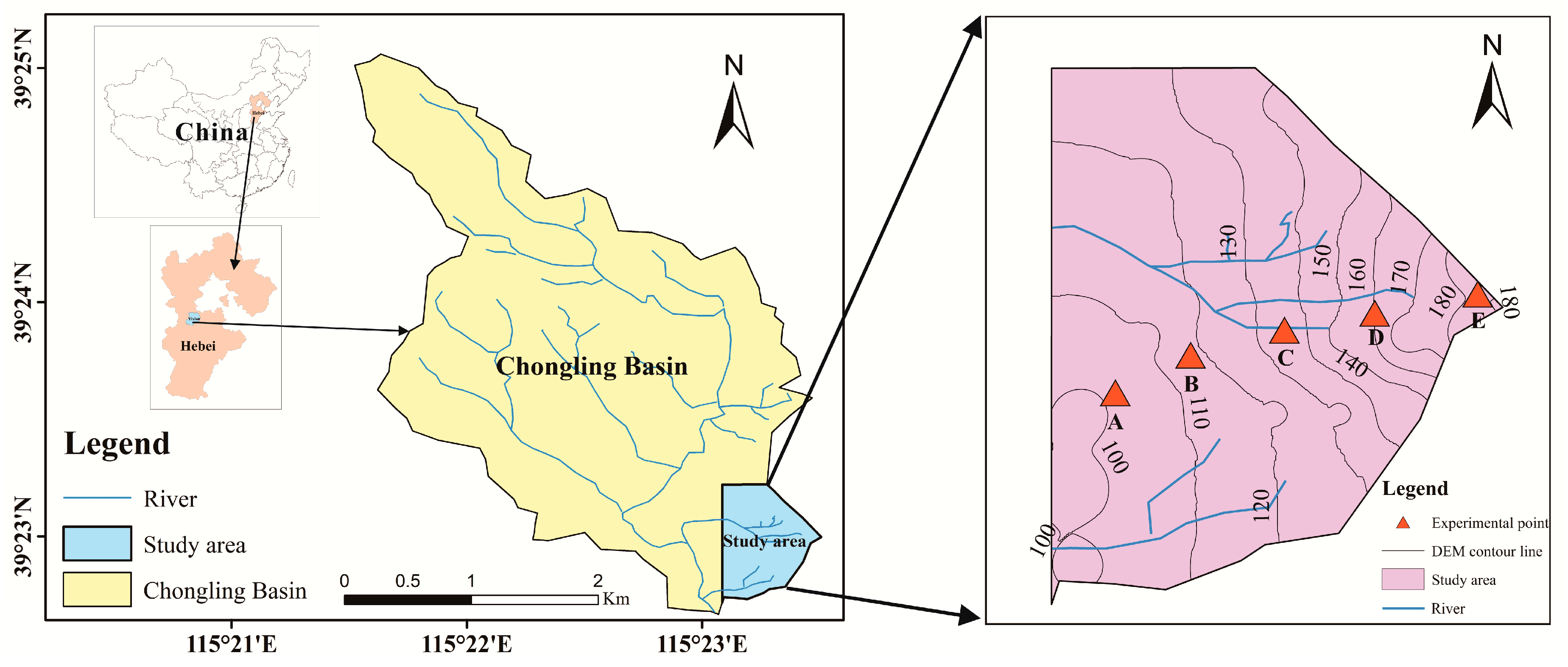
2.1. Study Area

The study area is the Chongling catchment area, which is located in the eastern part of the Yunmeng Mountains—A branch of the Taihang Mountains approximately 105 km southwest of Beijing, China (Figure 1). The Chongling watershed (115°21′–115°23′ E, 39°22′–39°25′ N) belongs to the secondary tributary of the northern Yishui River, and covers a total area of ~6 km2. There are five main river gullies in the watershed and the average river bed gradient is 23%. The landscape is characterized by low rolling hills and valleys with soil–stone mixtures. The altitude decreases from northwest to southeast and range from 85 m to 300 m. Geologically, there are limestone and marble in the northwest, purple–red conglomerate in the southeast, granitic gneiss weathering with a thickness of 1–3 m in the central area, and quaternary sediments composed of sand, clay, loess, and gravel in the valley area where the groundwater table is shallow at a depth of 2.5–4 m [43,44].
The Chongling watershed has a temperate continental monsoon climate. The annual precipitation in the study area ranges from 217.0 mm to 1004.3 mm, with an average of 641.2 mm. Affected by the East Asian monsoon, rainfall during the rainy season (usually between June and September) accounts for >70% of the total annual rainfall. The region is dry and cold during the winter with an average temperature of −7.2 °C, and hot and humid during the summer with an average temperature of 32.2 °C. The annual evapotranspiration (measured by evaporating dishes) is 1905.9 mm/year, >45% of which occurs between April and June due to the aridity and high temperatures [43,44].
The vegetation in the watershed is relatively well protected with high coverage and abundant vegetation types because the region was chosen as the Qing Dynasty Royal Tombs. Due to measures taken to enclose the hills for natural grassing or afforestation in the upstream hillside area, the vegetation coverage is generally 70–80% and mainly includes communities of Eriophorum brachyantherum and Angelica keiskei with shrubs such as Vitex negundo L. and Ziziphus jujuba Mill. The downstream hillside areas are mainly planted forests and nursery fields that include Platycladus orientalis, Pinus tabulaeformisCarr., Robinia pseudoacacia Linn., and Populus tomentosa Carr. The area of cultivated land is lesser and is mainly distributed in the valley area.

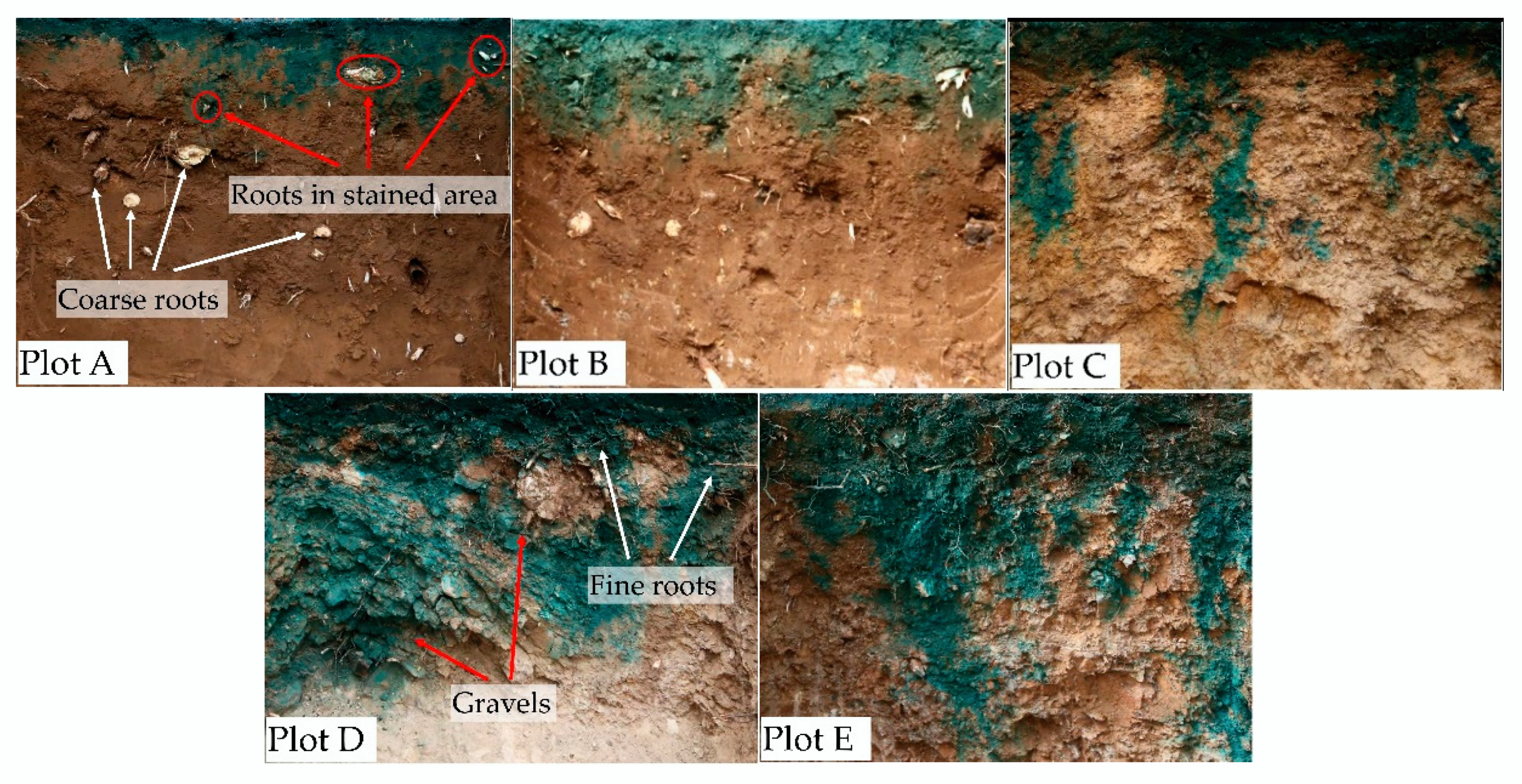
2.2. Experimental Procedure

The field campaign was conducted in May 2018. A representative hillslope in the southeast of the Chongling watershed near its outlet was selected as a typical hillslope to conduct dye experiments with the aim of evaluating the degree of preferential flow and infiltration redistribution at different hillslope positions. Five sample plots were established (A: bottom–, B: lower–, C: mid–, D: upper–, and E: top–slope positions) (Figure 1 and Figure 2, Table 1) and dye experiments were performed using BBFCF and KI–starch in each plot. The experimental plots were located at least 1.5 m from trees to reduce the interference from roots. There had been little rainfall in the two weeks before and during the experiments.
Before the dye experiments, the hillslope surface was flattened and vegetation (e.g., grass, shrubs and fallen leaves) on the surface were carefully removed. On each prepared plot, a rectangle frame made of polymethyl methacrylate (80 cm length × 60 cm width × 30 cm height) was embedded 10 cm into the soil, as illustrated in Figure 2. The soil on both sides of the frame was tamped by a wooden hammer in case of preferential infiltration along the inner wall of the frame.
BBFCF and KI–starch (colorized by spraying a starch solution) were selected as the staining tracers due to their high visibility in soils, ease of dissolution, and relatively low toxicity to the environment [15,45]. BBFCF is only accessible to infiltration paths with a larger diameter because the particles have a relatively large diameter and are easily blocked or absorbed by the soil matrix. However, negative monovalent iodide ions of the KI dye are easily soluble in water and are hardly absorbed by the soil matrix nor cause an obstruction. Hence, in this study, the soil sections stained by BBFCF demonstrated a pattern of preferential flow that was channeled via large pores, whereas those stained by KI–starch demonstrated the actual pattern of water infiltration. Thirty liters of mixed solution containing BBFCF (4 g/L) [15] and KI (10 g/L) [46] was sprayed evenly through a rainfall sprinkler for each plot. According to pre–tests, the simulated rainfall/dye intensity was set at 18 mm/h to avoid ponded or running water on the ground. After the simulated rainfall, the quadrat area was covered with waterproofing and insulation materials to prevent moisture from evaporating. After 24 h, the cover materials and polymethyl methacrylate frame were carefully removed.
Immediately after the remove of the cover and frame, seven vertical soil sections were excavated at each plot to a depth of 80 cm in 10 cm intervals starting from the lower edge along the hillslope (Figure 2); hence, a total of 35 vertical soil sections were obtained (Figure 3). After the excavation of each section, a rectangle scale frame made of aluminum alloy and a cubic white balance calibrator were placed on the section for the correction of geometric distortion and color analysis of images. Firstly, the soil section stained by BBFCF was photographed by a Canon digital camera under a shading plate (Figure 2). Then, the color developing agent containing ferric nitrate (25 g/L) and water–soluble starch (50 g/L) was evenly sprayed on the vertical soil section [46]. After the complete development of colors (~20 min), the soil section stained by KI–starch was also photographed from the same position as for the BBFCF staining. Earthworms and other soil-dependent animals were not observed during the excavation. Bulk density (BD), saturated hydraulic conductivity (Ks), field capacity (FC), saturated soil content (θsat) and soil particle size were measured with the soil samples collected by cutting ring with a volume of 100 m3 in different layers of soil. Meanwhile, about 10 kg mixed soil samples (including lager gravels) from different depths were collected to measure the gravel mass ratio (GMR), which is equal to the ratio of the mass of the dried gravels (>2 mm) to that of the total dried soil sample, to reduce the underestimation due to the limited volume of cutting ring (Table 2). The stable infiltrability was also estimated by means of curving fitting to Philip’s equation using double ring infiltrometers near the experimental plot during the act of excavation [47].

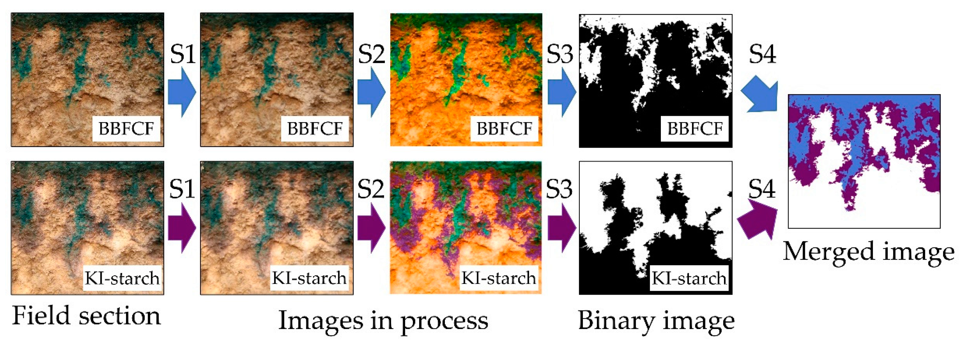
2.3. Image Analysis Techniques

Geometric distortion occurred when the stained sections were photographed with a digital camera. Therefore, the geometrical correction of the images was performed firstly by establishing a relationship between the location of the pixels in the image and the corresponding coordinates on the soil section [15], and the size of the image was set as 8 cm × 8 cm to embody the vertical soil section with a practical size of 80 cm × 80 cm. The image resolution was set as 100 pixels/cm and the total pixels per image was 800 × 800. A series of image analysis procedure for an image of a vertical soil section (Figure 4) was conducted to extract available data for calculation and evaluation. The image recordings of the soil sections that were stained by either BBFCF or KI–starch were treated in the same way, and the processing methods of the stained section images obtained under the two different dying treatments were also the same. The abundance of roots were measured with the method of image processing. The root distributing in the soil vertical section were recognized, color-replaced from the digital image and the pixels of roots were then extracted from the binary image. The abundance of roots (Φroot) were calculated as the proportion of root pixels in the whole section. The maximum depth of the roots (Droot) were also measured (Table 1).

2.4. Preferential Flow Indices

Dye coverage, DC (%), is defined by Flury et al. [45] as the percent coverage of the stained area. The DC at some depth, h, and the total DC (TotDC) of the soil section were calculated using Equations (1) and (2) respectively:
DC h = D h D h + UD h × 100 %
TotDC = Σ h = 0   80 DC h × 100 %
where Dh is the number of dye–stained pixels at the depth of h, and UDh is the unstained pixels on the depth of h.
The maximum infiltration depth, MaxID (cm), is the maximum penetration depth of dying tracer solution on the soil section. The uniform infiltration depth, UniID (cm), was defined by van Schaik [48] as the depth where the stained area strongly decreases, thus presenting the depth of the uniform infiltration front above which the infiltration process is dominated by uniform flow [26]. The depth of 80% of the DC is usually selected as the critical depth to divide the uniform flow area and the preferential flow area [21,26,48].
The preferential flow fraction, PF–fr, is the fraction of the total infiltration that flows through preferential flow paths [48]. The calculation method for the PF–fr was widely used in previous studies that only relied on the UniID as the boundary between the matrix flow area and the priority flow area [20,21,26,48,49]. However, the traditional calculation can lead to the inability to truly and completely distinguish the priority flow from the matrix flow. The first limitation of previous approaches is that they all used BBFCF as a single tracer for the analysis and calculation. As mentioned, during the process of infiltration with water flow, BBFCF particles are easily adsorbed and blocked by the soil matrix, and the redistribution process results in obvious hysteresis when compared with the actual water flow. The use of KI–starch could greatly reduce hysteresis and more accurately simulate the actual distribution of water flow. Another limitation is the imprecise division of the matrix flow region and priority flow region into upper and lower parts. A considerable portion of water flow is transversely diffused through the matrix during rapid infiltration via macropore channels. Although BBFCF dye can mark the macropore channels, it can hardly trace the part of water flowing horizontally through the macropore channel. The use of KI–starch tracer can, however, compensate for the above limitations. Hence, the present study modified the method of predecessors by simultaneous tracing with BBFCF and KI–starch. The matrix flow region is defined here as including the piston matrix flow region above the UniID (DC = 80%) and the transverse diffusion region, which represents the portion stained by the KI–starch while unstained by the BBFCF dye below the UniID in the KI–stained image.
When MaxIDBBFCFUniIDKI–starch, the modified calculation of the PF–fr is calculated using Equation (3); when MaxIDBBFCF < UniIDKI–starch, the modified calculation of the PF–fr is calculated using Equation (4).
PF fr = 1 Σ h = 0 UniID KI starch DC ( KI starch , h ) + Σ h = UniID KI starch MaxID KI starch ( DC ( KI starch , h ) DC ( BBFCF , h ) ) TotStAR KI starch × 100 %
PF fr = 1 Σ h = 0 UniID KI starch DC ( KI starch ,   h ) TotStAR KI starch × 100 %
where TotStARKI–starch is the total area stained by the KI–starch (cm2).

2.5. Evaluation of Infiltration Spatial Redistribution

2.5.1. Non–Uniformity Analysis of Infiltration Depth

In the tracer experiment, the vertical soil sections were not completely stained above the maximum staining depth due to flow inhomogeneity. Therefore, the actual staining depth can replace the maximum staining depth as recommended by others [17]. However, in the vertical section, the difference between the above two depths on the vertical section is mainly due to lateral infiltration, which is one of the important manifestations of preferential flow [32]. The replacement may fail to truly and completely describe the non–uniform characteristics of the preferential flow. Therefore, the non–uniformity coefficient (Cµ) of the preferential infiltration depth defined in this study is defined by Equation (5):
C μ = i = 1 N [ h max ( x i ,   y i ) h ¯ ] N · h ¯
where h max ( x i ,   y i ) is the maximum infiltration depth at ( x i ,   y i ) , h ¯ is the average of the maximum infiltration depth on a section, and N is total number of pixels parallel to (or orthogonal to) the section.

2.5.2. Fractal Dimension of the Preferential Flow Wetting Front

Fractal theory was first proposed by Mandelbrot [50], and was subsequently introduced by Tylor and Wheatcraft [51] for the study of soil science. The preferential flow wetting front trace recorded by the digital camera in the dye tracer experiment had distinct fractal features with obvious irregular, split, and disordered complex structures. In this study, the box–counting fractal dimension is used to describe the non–uniformity of the wetting front distribution in the two staining patterns. The method of calculating the box dimension involves first covering the wetting front by square pixel grids with a side length of δ. The number of boxes covered by the wetting front is N(δ), and then the fractal dimension, Df, is defined by Equation (6) [52]:
D f = lim δ 0 ln N ( δ ) ln δ
Df = 1 indicates that the wetting front is a straight line, thereby meaning that there is no preferential flow. Df > 1 indicates an irregular curve with the existence of preferential flow, and the value of Df is positively correlated with the non–uniformity of preferential flow. In this study, MATLAB was used to automatically calculate the Df of the wetting front, which is verified by the Koch curve and the Sierpinski triangle with high accuracy (relative error <5%).

2.6. Correlation and Error Analysis

Pearson’s correlation coefficient analysis was applied to investigate the correlations between the indices of preferential flow and spatial redistribution and environmental variables by using SPSS 18.0 software. The differences of the results were compared using one–way analysis of variance with SPSS 18.0 software.

3. Results and Discussion

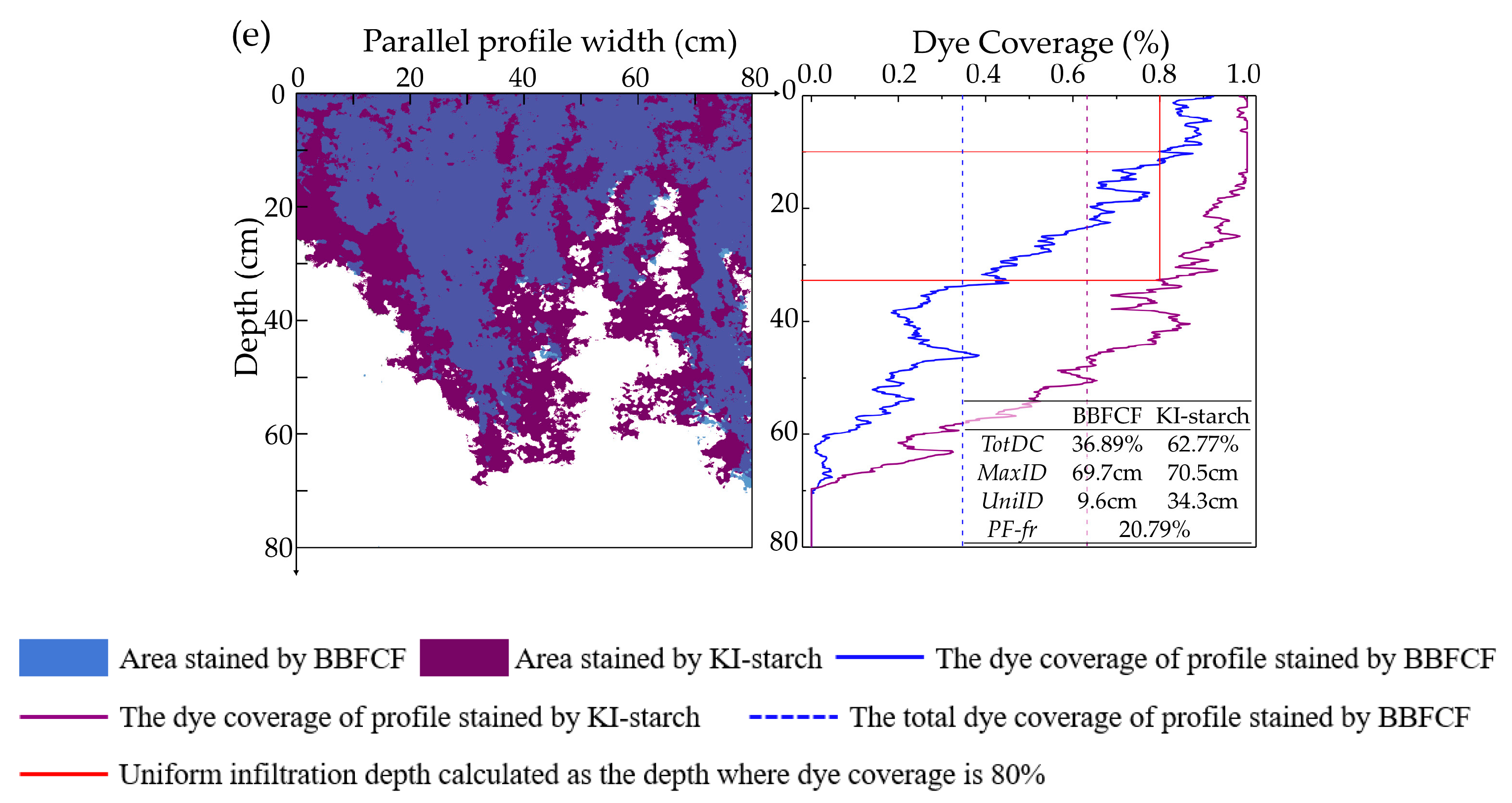
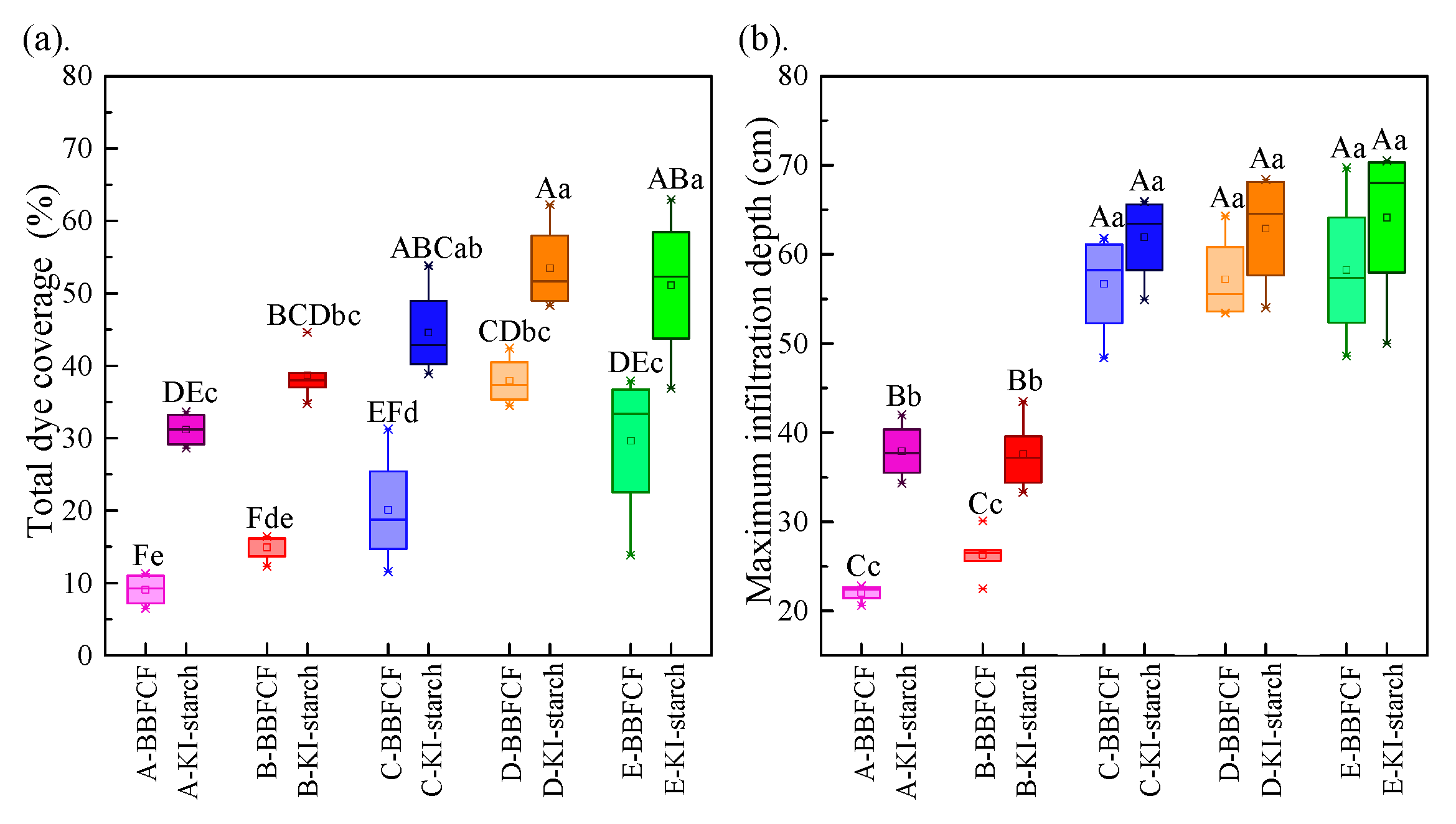
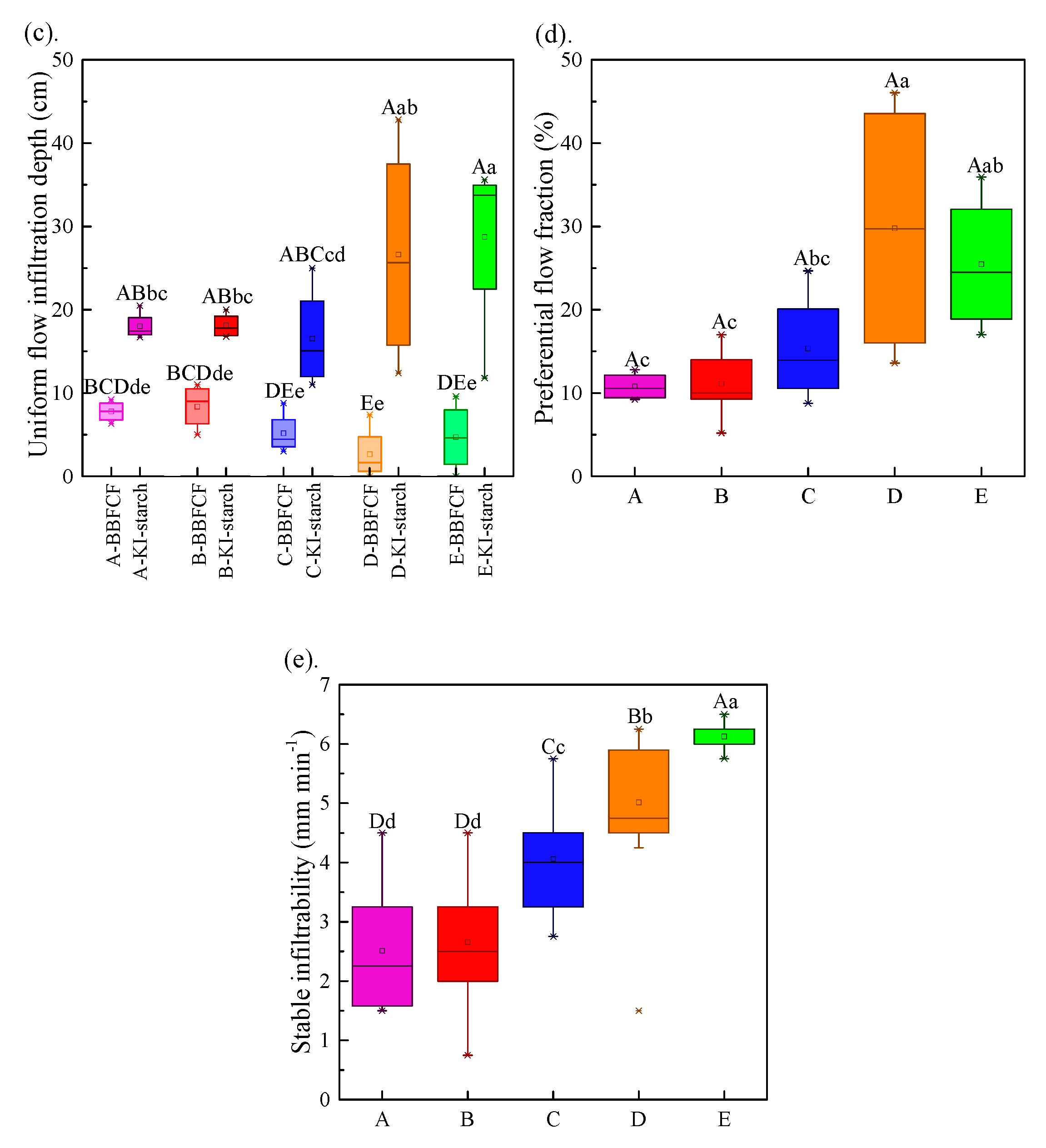
3.1. Degree of Preferential Flow

The two different dye tracers were applied to mark the pattern of soil water infiltration and redistribution on the experimental rocky hillslope. Thirty stained images of vertical soil sections on the five hillslope positions were investigated. Five representative stained section examples and their corresponding change in dye coverage with depth are presented in Figure 5.
The dye was distributed consistently throughout the area in a longitudinal direction at the bottom– and the lower–slope positions (Figure 5a,b). However, the stained area was distributed as the fingerlike, fragmented, and heterogeneous pattern on the mid–, upper–, and top–slope positions as evidenced by the existence of fingerlike extensions or the unstained fraction surrounded by a stained area (Figure 5c–e). In general, the purple KI–starch stained areas in Figure 5 are larger than the blue BBFCF stained areas, which implies that the infiltration flow distribution could not be recorded with a single dye tracer to estimate the degree of priority flow. The purple area is the extension and spread of the blue area, which indicates that soil water mainly infiltrated through some macropore channels and gradually diffused to the surrounding soil matrix. As mentioned, the negative monovalent iodide ions of the KI–starch dye are easily soluble in water and are hardly obstructed or absorbed by soil particles, which could be approximated as a representation of the actual flow [53]. Our results were consistent with those of Germán–Heins [54] and Jiang [55]. In addition, with increased elevation of the hillslope position, the blue area in Figure 5c–e occupies an increasing (previously purple in Figure 5a,b) area, which indicates that the contribution of priority flow to the actual water infiltration gradually increased with the elevation, and that preferential flow was the main contributor to soil water infiltration on the higher hillslope positions.
The variables of preferential flow treated with the two dye tracers on the different hillslope position are shown in Figure 6. The degree of preferential flow that was determined by the two dyes in addition to the soil steady infiltrability both increased with hillslope position (except for UniID with the BBFCF dye). All of the TotDC treated with KI–starch were significantly higher than those treated with the BBFCF dye, irrespective of the hillslope position. However, differences in the MaxID between the dye treatments among each of the higher hillslope plots were not statistically significant, while those between the bottom– and lower–slope plots were significant (p < 0.01). This indicates that a large fraction of the infiltrating dye tracer was channeled through preferential pathways, which is supported by the generally increasing trend of the modified PF–fr with increased hillslope position (bottom: 0.10; lower–slope: 0.11; mid–slope: 0.15; upper–slope: 0.29; top: 0.26). The mean value of the UniID, above which is generally defined as the region dominated by matrix piston flow, was 7.79, 8.36, 5.18, 2.68, and 3.19 cm for the BBFCF treatment and 18.02, 18.14, 16.53, 26.63, and 28.73 cm for the KI–starch treatment, from the bottom to the top of the hillslope, respectively. The mean values of stable infiltrability from the mid–slope to the top of the hillslope were 4.06, 5.01, and 6.13 mm min−1 and were significantly higher than that of the bottom (2.51 mm min−1) and lower–slope (2.65 mm min−1).
The variation range of each variable that is related to preferential flow also exhibited a gradually increasing trend with increased elevation, whereas the range of steady infiltrability was opposite. This indicates that infiltration channels, especially preferential channels, were more irregular in the upper– and top–slope positions and more uniform in the bottom–, lower–, and mid–slope plots.
The degree of preferential flow directly affects the infiltration capacity of water, and presents the more complex and chaotic redistribution pattern of water in soil [14,17,19]. Topographic factors can affect the infiltration process of soil water by influencing the physical and chemical properties of soil, soil thickness, and gravel content amongst others [23,24,26,34]. Even small topographic changes can cause drastic changes in soil conditions over a short distance. Hillslope position is an important terrain factor. With the increased elevation of the terrain, the soil layer became shallower, and the content of gravel increased with slower soil development and enhanced weathering (Table 2). Gravels with a diameter >30 mm were found to account for a larger proportion of the soil in the upper– and top–slope plots. The aforementioned increase in the degree of preferential flow with the rise of hillslope position agrees with the findings of Mei et al. [21], who suggested that the role of rock fragments and plant roots play an emphasized role in leading macropore flow. Macropores were determined by Alaoui et al. [6] to be more efficient at transporting water in comparison to piston flow.

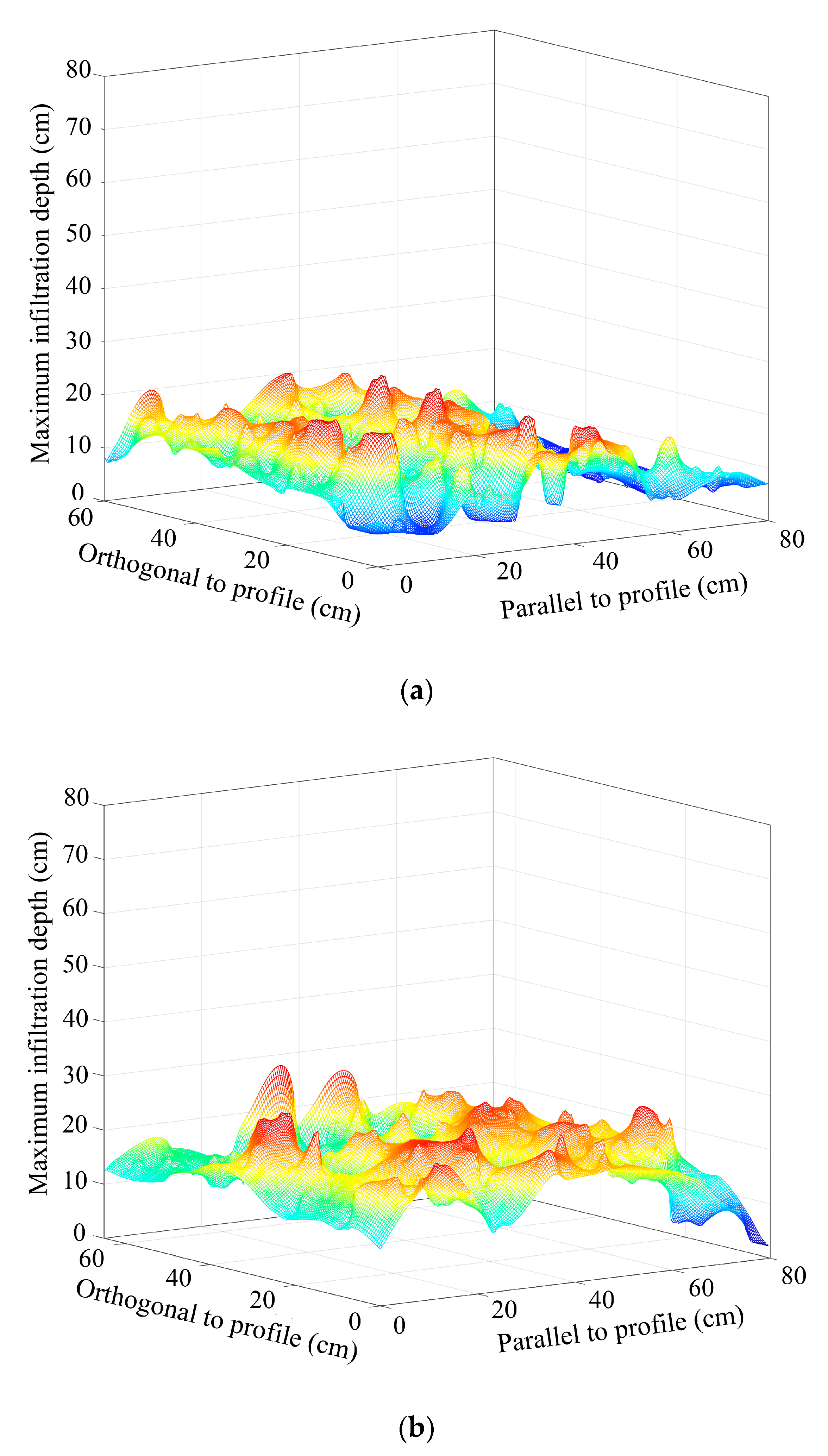
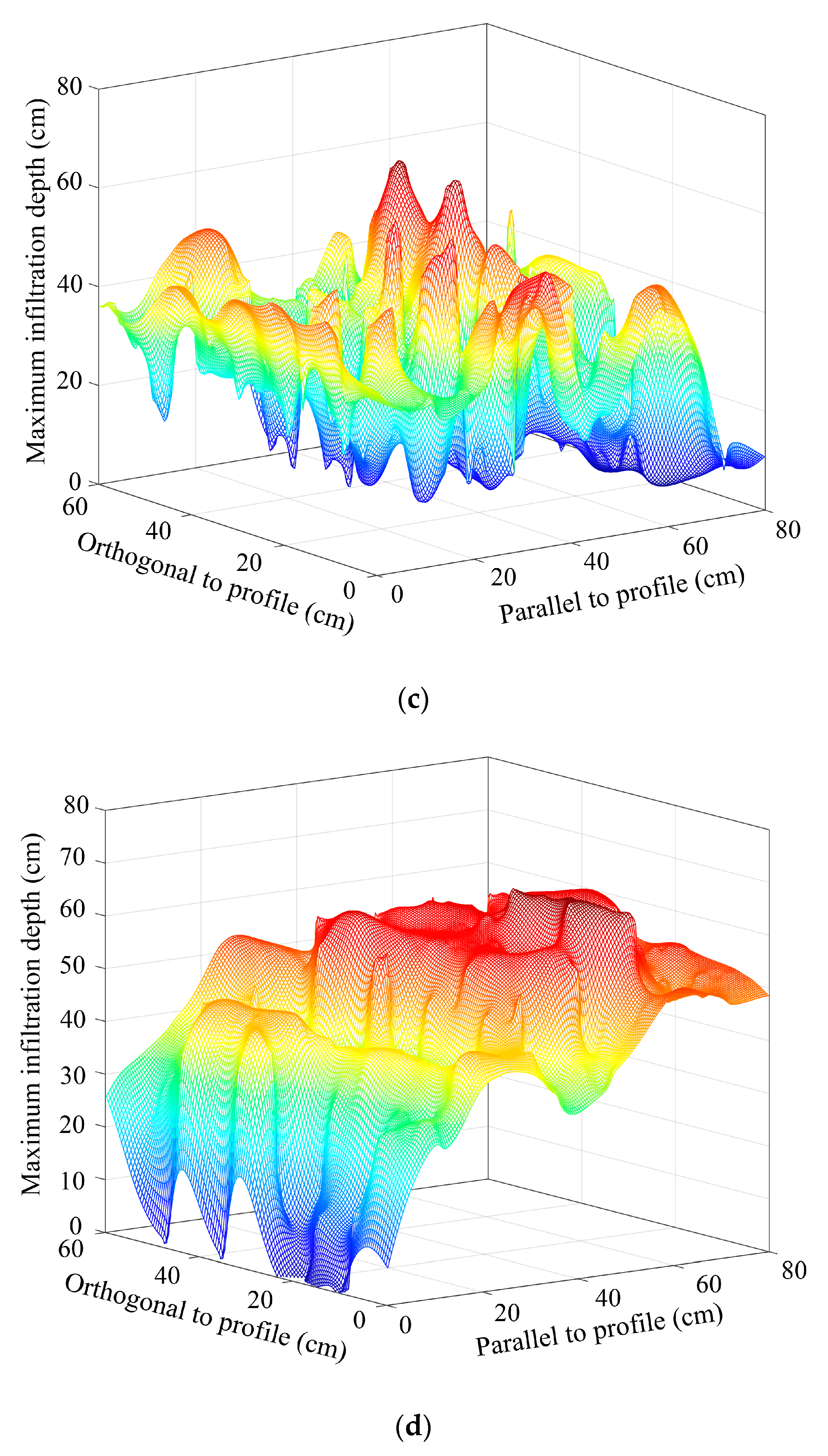
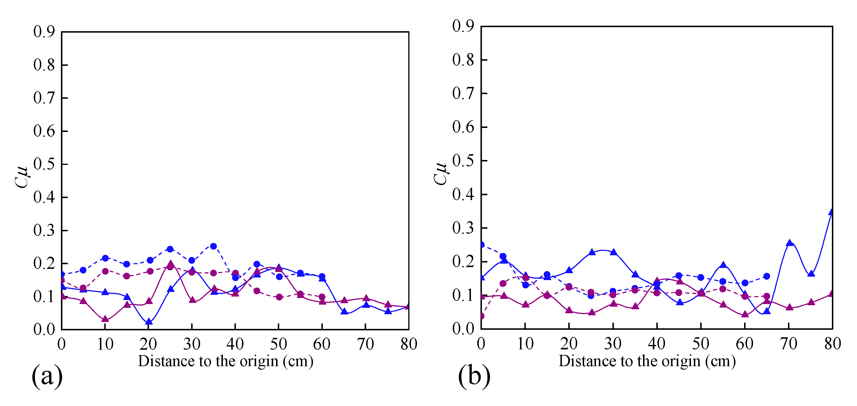
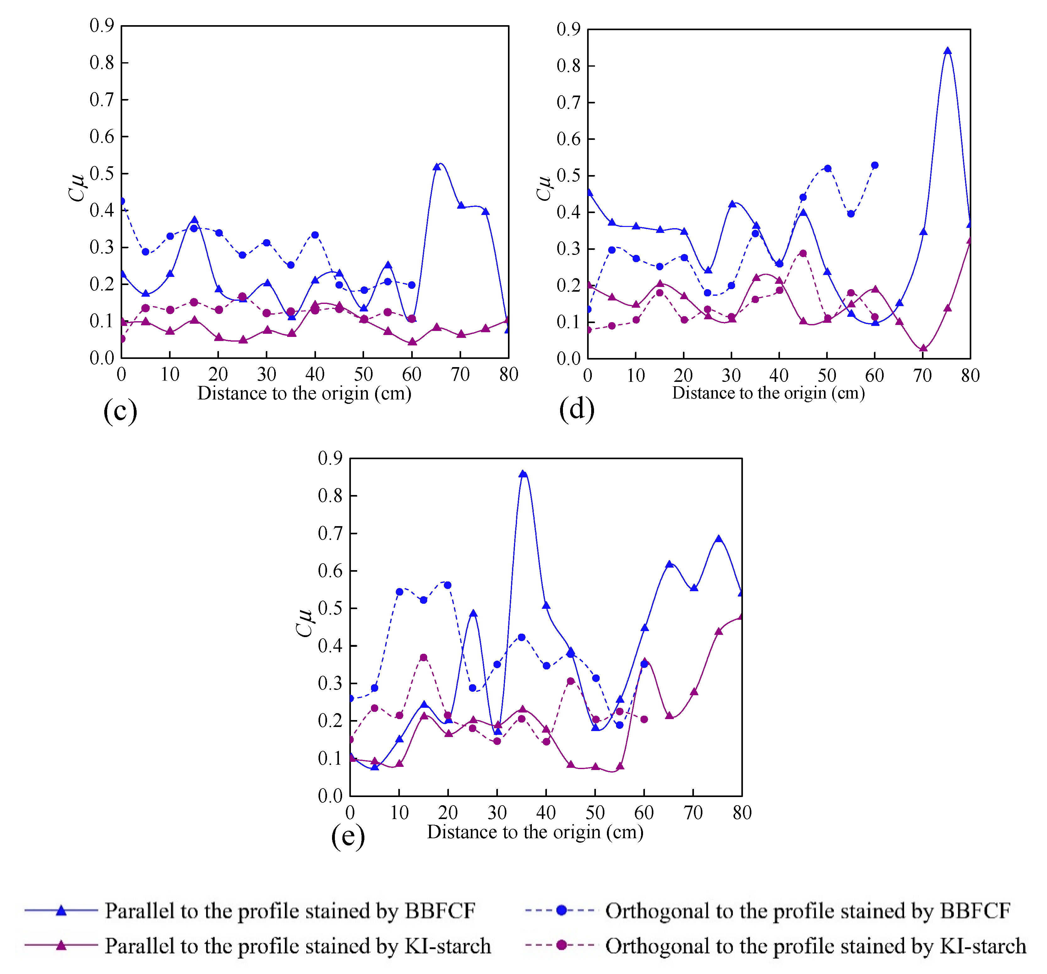
3.2. Spatial Redistribution of Infiltration

In order to reflect the spatial characteristics of soil water redistribution after infiltration, the ground surface of each experimental plot was discretized into a square grid of 0.1 cm × 0.1 cm, thereby obtaining 4.8 × 10⁶ square grids for each experiment. MATLAB was applied to draw a three–dimensional space contour of the maximum infiltration depth of each experimental plot (Figure 7). Great differences were observed in the soil water redistribution after infiltration between experimental plots/hillslope positions.
The Cμ of the infiltration depths were analyzed for each three–dimensional spatial distribution map along the parallel and orthogonal directions of the stained experimental soil cuboid (Figure 8). The solid line with a triangle in Figure 8 represents the variation of Cμ with the distance to the origin in the orthogonal direction (InOrD hereafter) to reflect the degree of heterogeneity in the infiltration depth between the dye–stained sections. The dashed lines with solid circles represent the variation of Cμ in the parallel direction (InPaD hereafter) to reflect the degree of internal heterogeneity in the dye–stained sections. The Cμ–distance curve in Figure 8a for the bottom of the hillslope was similar for the two dye treatments, whereby the orthogonal variation ranged from 0.02 to 0.18 and the parallel variation ranged from 0.11 to 0.28. In comparison to the Cμ InOrD, the Cμ InPaD yielded a higher value and less fluctuation. In Figure 8b for the lower–slope, the variation of the Cμ in the different directions and with the two dyes was consistent with that of Figure 8a, where the overall variation range was between 0.05 and 0.34. The increase of the Cμ fluctuation InOrD was observed for the BBFCF treatment. The Cμ–distance curve of the two dying treatments in Figure 8c show an obvious separation. The curve of the BBFCF dye fluctuates more (ranging from 0.14 to 0.52) than the curve of KI–starch, which maintained a relatively stable trend in both directions, and was closer to that of Figure 8a,b. In Figure 8d, the value and range of the Cμ for the BBFCF dye increases further, and both increase greatly InPaD and InOrD with increased distance to the origin. Meanwhile, the fluctuation of the curve for the KI–starch treatment also increased significantly, but was still more stable than that of the BBFCF dye. The maximum values of Cμ for the BBFCF and KI–starch treatments were found in Figure 8e to be 0.86 and 0.62, respectively. The fluctuation of the Cμ–distance curve also peaked while that for the different dying treatments remain separated.
To accurately compare the Cμ of the water flow infiltration depth at different hillslope positions and in different directions under different dying treatments, the statistical characteristic values of the Cμ curve in Figure 8 are summarized in Table 3.
With increased hillslope position, the statistical characteristic values of the Cμ (i.e., the average, Ave. Cμ, the range, Ran. Cμ, and the standard deviation, Std. Cμ) mainly showed a gradual increasing trend. Although some minimum values were evident for plot B (lower–slope), they were close to the corresponding values determined for plot A (bottom of the hillslope), for example, the Ave. Cμ of the BBFCF dye InOrD and the Ave. Cμ for the KI–starch treatment InPaD. This indicates that the non–uniformity of the spatial redistribution of the soil water infiltration gradually increased with the rise in the hillslope position. The stable curve of the Cμ for the bottom– (plot A) and lower–slopes (plot B) might have been due to a more homogeneous seepage medium. In this case, soil water would have been stored in the soil pores under molecular and capillary forces, thus making any transfer to the surrounding environment difficult [30]. The spatial redistribution of infiltration in the mid– and upper–slopes revealed more potential preferential channels that were caused by the heterogeneous soil structure. These trends were supported by the findings of Liu et al. [56], van Schaik et al. [48], and Öhrström et al. [57].
Comparison of the Cμ under different treatments in the same direction showed that all of the statistical characteristic values of the Cμ for the BBFCF dye were significantly higher than those of the KI–starch dye, which indicates that the spatial heterogeneity of the infiltration pattern recorded by the BBFCF dye was significantly larger than that of the KI–starch. Sheng et al. also found the infiltration of an ionic solution tracer revealed the spatial redistribution more accurately than that of a macromolecule solution [47], while the latter was better for detecting macropores channels. Moreover, the Cμ in different directions under the same treatment were compared, and showed that the Ave. Cμ InOrD was larger than that of the InPaD, while the Ran. Cμ and Std. Cμ presented the opposite trend, which might have represented the non–uniformity lateral flow pathway [32].
The fractal dimension (Df) values of the wet front curve of each plot for the two different dying treatments are shown in Table 4. The Df increased with increasing elevation regardless of the dye type. The larger the Df value, the higher the irregularity of the wet front curve, which further supported the influence of the hillslope position on the redistribution of infiltration [17]. In addition, the Df values for the BBFCF dye were generally larger than those for the KI–starch dye, which emphasized the role of water diffusion in the infiltration process with priority flow [1]. It is necessary to take the convection and diffusion of soil water movement into consideration in the study of matrix and priority flow.

3.3. Factors Impacting Preferential Flow and Infiltration Redistribution

The main environmental factors affecting the preferential flow and infiltration redistribution were assessed using the correlation coefficients between the environmental variables and indices of preferential flow and infiltration redistribution (Table 5).
In the BBFCF treatment, altitude, slope gradient, gravel mass ratio (GMR), soil saturated hydraulic conductivity (Ks), initial water content (θint), saturated water content (θsat), sand and the abundance of the roots in stained area (Φroot-stained) generally had a negative correlation with UniID and a positive correlation with other preferential and redistribution indices. Soil thickness (ST), bulk density (BD), clay, silt, the total abundance of roots (Φroot) and the maximum depth of roots (Droot) exhibited a positive correlation with UniID and a negative correlation with other indices. The relationships between altitude, BD, GMR, θsat, soil particle size and Φroot-stained and MaxID, UniID, Cμ, and Df showed varying levels of significantly correlation. Ks had a significant impact on the Cμ between sections. In the KI–starch treatment, ST, BD exhibited a negative correlation with preferential and redistribution indices, whereas some other environmental variables (altitude, gradient, GMR, Ks, θsat, Φroot-stained) exhibited positive correlations with those indices. The relationships between altitude, BD, GMR, Ks, soil particle size and Φroot-stained and TotDC, MaxID, and Df were significantly correlated. Furthermore, the correlation between BD, θsat, soil particle size and PF–fr was also significant (Table 5). In addition, the results showed that there is little correlation between θint, Φroot and Droot and the preferential flow and infiltration redistribution.
Preferential flow and infiltration redistribution were statistically affected by the GMR and BD. Gravels with a diameter of >30 mm were found in the soil layer on the middle– and upper–slope plots. Katra et al. [30] found that gravel with a diameter of >4.76 mm had a significantly greater impact on the soil infiltration rate than gravel with a diameter of 2.38–4.76 mm. In the uncompacted soil layer, an increased gravel content has been found to significantly increase the number of soil macropores, while the decrease of the overwater section and the increase in the water flow curvature have been shown to have lesser effects on the soil water inhibition [22,32]. In addition, the increased gravel content may also provide potential channels for the lateral soil midstream [32], thus manifesting the increase of the non–uniformity InOrD.
The GMR has also been found to indirectly affect the degree of priority flow and infiltration redistribution by changing the BD, Ks, and θsat amongst others [30]. The BD in the present study exhibited strong negative correlations with the degree of preferential flow and the spatial infiltration redistribution, which were consistent with the findings of Mei et al. [21], who demonstrated that the impact of BD was related to the total porosity. In addition, we found that Ks and θsat were strongly related to the infiltration process, especially with respect to spatial redistribution, which was supported by the results of Laine–Kaulio [58].
The correlation between the roots in stained area (Φroot-stained) and the indices of preferential flow and infiltration redistribution demonstrated that the impact of roots can not afford to be neglected. The plant roots were generally proved to change the soil properties by reducing bulk density and increasing soil properties, which is critically responsible for the depth and heterogeneity of infiltration [6,21,26]. However, there is little correlation between the total abundance of roots (Φroot) and the infiltration indices. The large differences between Φroot and Φroot-stained in Plots A and B were found, contrasting with those in Plots C, D, and E. As mentioned in Table 1, the main difference in surface vegetation types in Plots A and B from those in other higher plots is the Robinia pseudoacacia Linn. The root systems of Robinia pseudoacacia Linn were more deeply spread than those of shrubs [21], and there were coarse roots found in the soil vertical section (like the example of Plot A in Figure 3). However, stained spots were not found around the most of the roots in Plot A, especially around the coarse roots. In contrast, the vertical soli section exhibited more fine roots, particularly in the upper zone, and most of them were surrounded by dye tracer. These results agreed with those obtained by Mei [21], who indicated that root systems in the upper soil have more strong influence on preferential flow. However, Yunusa [59] indicated that roots pathways are deeper and wider under woody perennials compared to annual crops and pasture, contributing to enhance the preferential flow, which conflicted with our results. Limited amounts of simulated precipitation and denser soil texture might led to this confliction.

4. Conclusions

To evaluate spatial variation of the degree of preferential flow and infiltration redistribution on different hillslope positions, dye tracer experiments were performed at the bottom–, lower–, mid–, upper–, and top–slope positions on a representative hillslope in the rocky Taihang Mountains. The dye tracer solution was mixed with BBFCF and KI–starch to distinguish the flow patterns of macropore flow and actual water flow. The three main conclusions of this study are as follows:
(1)
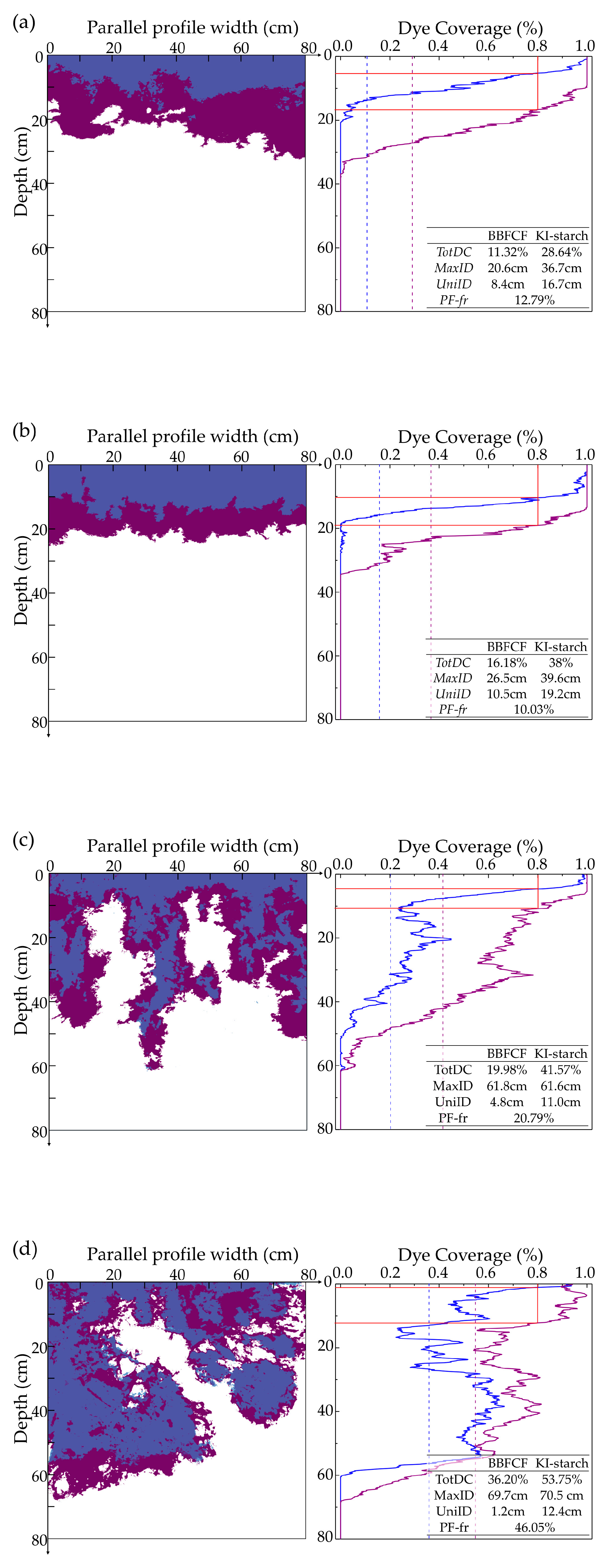
With increasing hillslope position, the total dye coverage, maximum infiltration depth, and saturation steady infiltration rate all showed obvious increasing trends; the contribution of preferential flow to the actual water infiltration gradually increased with plot elevation, whereby the value of the mean preferential flow fraction (PF-fr) was 0.10, 0.11, 0.15, 0.29, and 0.26 for the bottom–, lower–, mid–, upper–, and top–slope positions, respectively.
(2)
The non–uniformity of the spatial redistribution of the soil water infiltration gradually increased with the rise in hillslope position. The mean non-uniformity coefficient (Cμ) of the actual water infiltration maximum depth at the bottom–, lower–, mid–, upper–, and top–slope positions was 0.12, 0.12, 0.14, 0.16, and 0.24 in orthogonal direction to the stained section, and 0.10, 0.08, 0.17, 0.15, and 0.19 in the parallel section direction, respectively. The dimension fraction (Df) value of the actual water infiltration wet front curve for five hillslope positions was 1.2015, 1.2561, 1.3257, 1.3525, and 1.4055 for the bottom–, lower–, mid–, upper–, and top–slope positions, respectively. Additionally, the degree of non–uniformity of the spatial redistribution for macropore flow revealed by the BBFCF dying pattern was larger than that of the actual water flow revealed by the KI–starch dying pattern.
(3)
The GMR, θsat, altitude, Ks, Φroot-stained were found to be the main positive factors impacting the degree of preferential flow and spatial non–uniformity of the infiltration redistribution. A lower BD and lower clay content could effectively promote preferential flow and the spatial distribution of heterogeneity.
The preferential flow and infiltration redistribution exhibited significant spatial variability along a hillslope in the rocky mountain area. It is necessary to take the contribution of preferential flow and heterogeneous infiltration into consideration, particularly in the application and modification of numerical modeling which is worthy further studying. Our findings therefore provide information for other researchers investigating the infiltration process of preferential flow in rocky mountain areas and reference for parameter application and selection, contributing to the improvement of simulation accuracy of montane hydrological models.

Author Contributions

All authors contributed to the conception and development of this manuscript. S.-y.Z. and Y.-w.J. carried out the analysis and wrote the paper. J.-g.G. and C.-w.N. designed the experimental scheme and developed the project implementation plan. S.-y.Z. and H.-d.S. carried out the dye tracer experiment and image analysis process. Y.-d.G. and H.L. participated in the results analysis and diagram drawing. All authors have read and agreed to the published version of the manuscript.

Funding

This study was supported by the National High-level Talent Special Support Fund of China (WR0166A012019), the Projects of the National Science Foundation of China (51779272, 51909129), the Natural Science Foundation of Qinghai Province of China (2018-ZJ-965Q), and the National Basic Research Program of China (973 Program) (2015CB452701).

Conflicts of Interest

The authors declare no conflict of interest.

References

  1. Zhao, N.; Yu, F.; Li, C.; Wang, H.; Liu, J.; Mu, W. Investigation of rainfall–runoff processes and soil moisture dynamics in grassland plots under simulated rainfall conditions. Water 2014, 6, 2671–2689. [Google Scholar] [CrossRef] [Green Version]
  2. Mu, W.; Yu, F.; Li, C.; Xie, Y.; Tian, J.; Liu, J.; Zhao, N. Effects of rainfall intensity and slope gradient on runoff and soil moisture content on different growing stages of spring maize. Water 2015, 7, 2990–3008. [Google Scholar] [CrossRef] [Green Version]
  3. Allaire, S.E.; Roulier, S.; Cessna, A.J. Quantifying preferential flow in soils: A review of different techniques. J. Hydrol. 2009, 378, 179–204. [Google Scholar] [CrossRef]
  4. Beven, K.; Germann, P. Macropores and water flow in soils. Water Resour. Res. 1982, 18, 1311–1325. [Google Scholar] [CrossRef] [Green Version]
  5. Capuliak, J.; Pichler, V.; Flühler, H.; Pichlerová, M.; Homolák, M. Beech forest density control on the dominant water flow types in andic soils. Vadose Zone J. 2010, 9, 747–756. [Google Scholar] [CrossRef]
  6. Alaoui, A.; Caduff, U.; Gerke, H.H.; Weingartner, R. Preferential flow effects on infiltration and runoff in grassland and forest soils. Vadose Zone J. 2011, 10, 367–377. [Google Scholar] [CrossRef]
  7. Peters, D.L.; Buttle, J.M.; Taylor, C.H.; LaZerte, B.D. Runoff production in a forested shallow soil, Canadian Shield basin. Water Resour. Res. 1995, 31, 1291–1304. [Google Scholar] [CrossRef]
  8. Van der Heijden, G.; Legout, A.; Pollier, B.; Bréchet, C.; Ranger, J.; Dambrine, E. Tracing and modeling preferential flow in a forest soil—Potential impact on nutrient leaching. Geoderma 2013, 195–196, 12–22. [Google Scholar] [CrossRef]
  9. Jarvis, N.; Etana, A.; Stagnitti, F. Water repellency, near–saturated infiltration and preferential solute transport in a macroporous clay soil. Geoderma 2008, 143, 223–230. [Google Scholar] [CrossRef]
  10. Jomaa, S.; Barry, D.A.; Heng, B.C.P.; Brovelli, A.; Sander, G.C.; Parlange, J.Y. Effect of antecedent conditions and fixed rock fragment coverage on soil erosion dynamics through multiple rainfall events. J. Hydrol. 2013, 484, 115–127. [Google Scholar] [CrossRef]
  11. Zhang, J.; Lei, T.; Qu, L.; Chen, P.; Gao, X.; Chen, C.; Yuan, L.; Zhang, M.; Su, G. Method to measure soil matrix infiltration in forest soil. J. Hydrol. 2017, 552, 241–248. [Google Scholar] [CrossRef]
  12. Bouma, J.; Belmans, C.F.M.; Dekker, L.W. Water infiltration and redistribution in a silt loam subsoil with vertical worm channels1. Soil Sci. Soc. Am. J. 1982, 46, 917–921. [Google Scholar] [CrossRef]
  13. Ritsema, C.J.; Dekker, L.; Hendrickx, J.M.H.; Hamminga, W. Preferential flow mechanism in a water repellent sandy soil. Water Resour. Res. 1993, 29, 2183–2194. [Google Scholar] [CrossRef]
  14. Gerke, H.H. Preferential flow descriptions for structured soils. J. Plant Nutri. Soil Sci. 2006, 169, 382–400. [Google Scholar] [CrossRef]
  15. Weiler, M.; Flühler, H. Inferring flow types from dye patterns in macroporous soils. Geoderma 2004, 120, 137–153. [Google Scholar] [CrossRef]
  16. Hagedorn, F.; Bundt, M. The age of preferential flow paths. Geoderma 2002, 108, 119–132. [Google Scholar] [CrossRef]
  17. Sheng, F.; Wang, K.; Zhang, R.; Liu, H. Characterizing soil preferential flow using iodine—Starch staining experiments and the active region model. J. Hydrol. 2009, 367, 115–124. [Google Scholar] [CrossRef] [Green Version]
  18. Weiler, M.; Naef, F. Simulating surface and subsurface initiation of macropore flow. J. Hydrol. 2003, 273, 139–154. [Google Scholar] [CrossRef]
  19. Alaoui, A.; Helbling, A. Evaluation of soil compaction using hydrodynamic water content variation: Comparison between compacted and non–compacted soil. Geoderma 2006, 134, 97–108. [Google Scholar] [CrossRef]
  20. Kan, X.; Cheng, J.; Hu, X.; Zhu, F.; Li, M. Effects of grass and forests and the infiltration amount on preferential flow in karst regions of China. Water 2019, 11, 1634. [Google Scholar] [CrossRef] [Green Version]
  21. Mei, X.; Zhu, Q.; Ma, L.; Zhang, D.; Wang, Y.; Hao, W. Effect of stand origin and slope position on infiltration pattern and preferential flow on a Loess hillslope. Land Degrad. Dev. 2018, 29, 1353–1365. [Google Scholar] [CrossRef]
  22. Dadkhah, M.; Gifford, G.F. Influence of vegetation, rock cover, and trampling on infiltration rates and sediment production. J. Am. Water Resour. Assoc. 1980, 16, 979–986. [Google Scholar] [CrossRef]
  23. Liu, C.; Cheng, S.; Yu, W.; Chen, S. Water infiltration rate in cracked paddy soil. Geoderma 2003, 117, 169–181. [Google Scholar] [CrossRef]
  24. Navar, J.; Mendez, J.; Bryan, R.B.; Kuhn, N.J. The contribution of shrinkage cracks to bypass flow during simulated and natural rainfall experiments in northeastern Mexico. Can. J. Soil Sci. 2002, 82, 65–74. [Google Scholar] [CrossRef] [Green Version]
  25. Li, T.; Shao, M.A.; Jia, Y. Effects of activities of ants (Camponotus japonicus) on soil moisture cannot be neglected in the northern Loess Plateau. Agric. Eco. Environ. 2017, 239, 182–187. [Google Scholar] [CrossRef]
  26. Bargués Tobella, A.; Reese, H.; Almaw, A.; Bayala, J.; Malmer, A.; Laudon, H.; Ilstedt, U. The effect of trees on preferential flow and soil infiltrability in an agroforestry parkland in semiarid Burkina Faso. Water Resour. Res. 2014, 50, 3342–3354. [Google Scholar] [CrossRef] [PubMed] [Green Version]
  27. Zhou, B.B.; Shao, M.A.; Wang, Q.J.; Yang, T. Effects of different rock fragment contents and sizes on solute transport in soil columns. Vadose Zone J. 2011, 10, 386–393. [Google Scholar] [CrossRef]
  28. Oshun, J.; Dietrich, W.E.; Dawson, T.E.; Fung, I. Dynamic, structured heterogeneity of water isotopes inside hillslopes. Water Resour. Res. 2016, 52, 164–189. [Google Scholar] [CrossRef] [Green Version]
  29. Mol, L.; Viles, H.A. Geoelectric investigations into sandstone moisture regimes: Implications for rock weathering and the deterioration of San Rock Art in the Golden Gate Reserve, South Africa. Geomorphology 2010, 118, 280–287. [Google Scholar] [CrossRef]
  30. Katra, I.; Lavee, H.; Sarah, P. The effect of rock fragment size and position on topsoil moisture on arid and semi–arid hillslopes. Catena 2008, 72, 49–55. [Google Scholar] [CrossRef]
  31. Oostwoud Wijdenes, D.J.; Poesen, J. The effect of soil moisture on the vertical movement of rock fragments by tillage. Soil Tillage Res. 1999, 49, 301–312. [Google Scholar] [CrossRef]
  32. Zhang, Y.; Zhang, M.; Niu, J.; Li, H.; Xiao, R.; Zheng, H.; Bech, J. Rock fragments and soil hydrological processes: Significance and progress. Catena 2016, 147, 153–166. [Google Scholar] [CrossRef]
  33. Sepaskhah, A.R.; Tafteh, A. Pedotransfer function for estimation of soil–specific surface area using soil fractal dimension of improved particle–size distribution. Arch. Agron. Soil Sci. 2013, 59, 93–103. [Google Scholar] [CrossRef]
  34. Hlaváčiková, H.; Holko, L.; Danko, M.; Novák, V. Estimation of macropore flow characteristics in stony soils of a small mountain catchment. J. Hydrol. 2019, 574, 1176–1187. [Google Scholar] [CrossRef]
  35. Nimmo, J.R.; Creasey, K.M.; Perkins, K.S.; Mirus, B.B. Preferential flow, diffuse flow, and perching in an interbedded fractured–rock unsaturated zone. Hydrogeol. J. 2017, 25, 421–444. [Google Scholar] [CrossRef]
  36. Fu, Z.Y.; Chen, H.S.; Zhang, W.; Xu, Q.X.; Wang, S.; Wang, K.L. Subsurface flow in a soil–mantled subtropical dolomite karst slope: A field rainfall simulation study. Geomorphology 2015, 250, 1–14. [Google Scholar] [CrossRef]
  37. Corwin, D.L.; David, A.; Goldberg, S. Mobility of arsenic in soil from the Rocky Mountain Arsenal area. J. Contam. Hydrol. 1999, 39, 35–58. [Google Scholar] [CrossRef]
  38. Han, S.; Yang, Y.; Fan, T.; Xiao, D.; Moiwo, J.P. Precipitation–runoff processes in Shimen hillslope micro–catchment of Taihang Mountain, north China. Hydrol. Process. 2012, 26, 1332–1341. [Google Scholar] [CrossRef]
  39. Liu, Z.; Yu, X.; Jia, G.; Jia, J.; Lou, Y.; Lu, W. Contrasting water sources of evergreen and deciduous tree species in rocky mountain area of Beijing, China. Catena 2017, 150, 108–115. [Google Scholar] [CrossRef]
  40. Du, J.; Jia, Y.; Hao, C.; Qiu, Y.; Niu, C.; Liu, H. Temporal and spatial changes of blue water and green water in the Taihang Mountain Region, China, in the past 60 years. Hydrol. Sci. J. 2019, 64, 2040–2056. [Google Scholar] [CrossRef]
  41. Xu, F.; Jia, Y.; Peng, H.; Niu, C.; Liu, J.; Hao, C.; Huang, G. Vertical zonality of the water cycle and the impact of land–use change on runoff in the Qingshui River Basin of Wutai Mountain, China. Hydrol. Sci. J. 2019, 64, 2080–2092. [Google Scholar] [CrossRef]
  42. Li, F.; Song, X.; Tang, C.; Liu, C.; Yu, J.; Zhang, W. Tracing infiltration and recharge using stable isotope in Taihang Mt., North China. Environ. Geol. 2007, 53, 687–696. [Google Scholar] [CrossRef]
  43. Song, X.; Wang, P.; Yu, J.; Liu, X.; Liu, J.; Yuan, R. Relationships between precipitation, soil water and groundwater at Chongling catchment with the typical vegetation cover in the Taihang mountainous region, China. Environ. Earth Sci. 2011, 62, 787–796. [Google Scholar] [CrossRef]
  44. Yu, J.; Yang, C.; Liu, C.; Song, X.; Hu, S.; Li, F.; Tang, C. Slope runoff study in situ using rainfall simulator in mountainous area of North China. J. Geogr. Sci. 2009, 19, 461–470. [Google Scholar] [CrossRef]
  45. Flury, M.; Flühler, H.; Jury, W.A.; Leuenberger, J. Susceptibility of soils to preferential flow of water—A field study. Water Resour. Res. 1994, 30, 1945–1954. [Google Scholar] [CrossRef]
  46. Sheng, F.; Liu, H.; Zhang, R.; Wang, K. Determining the active region model parameter from dye staining experiments for characterizing the preferential flow heterogeneity in unsaturated soils. Environ. Earth Sci. 2012, 65, 1977–1985. [Google Scholar] [CrossRef]
  47. Bamutaze, Y.; Tenywa, M.M.; Majaliwa, M.J.G.; Vanacker, V.; Bagoora, F.; Magunda, M.; Obando, J.; Wasige, J.E. Infiltration characteristics of volcanic sloping soils on Mt. Elgon, Eastern Uganda. Catena 2010, 80, 122–130. [Google Scholar] [CrossRef]
  48. Van Schaik, N.L.M.B. Spatial variability of infiltration patterns related to site characteristics in a semi–arid watershed. Catena 2009, 78, 36–47. [Google Scholar] [CrossRef]
  49. Gerke, K.M.; Sidle, R.C.; Mallants, D. Preferential flow mechanisms identified from staining experiments in forested hillslopes. Hydrol. Process. 2015, 29, 4562–4578. [Google Scholar] [CrossRef]
  50. Mandelbrot, B. How long is the coast of Britain? Statistical self–similarity and fractional dimension. Science 1967, 156, 636–638. [Google Scholar] [CrossRef] [Green Version]
  51. Tyler, S.W.; Wheatcraft, S.W. Fractal scaling of soil particle–size distributions: Analysis and limitations. Soil Sci. Soc. Am. J. 1992, 56, 362–369. [Google Scholar] [CrossRef]
  52. Falconer, K. Fractal Geometry—Mathematical Foundations and Applications, 4th ed.; Northeastern University Press: Shenyang, China, 1996; pp. 56–77. [Google Scholar]
  53. Flury, M. Dyes as tracers for vadose zone hydrology. Rev. Geophys. 2003, 41, 2. [Google Scholar] [CrossRef]
  54. Germán–Heins, J.; Flury, M. Sorption of Brilliant Blue FCF in soils as affected by pH and ionic strength. Geoderma 2000, 97, 87–101. [Google Scholar] [CrossRef]
  55. Jiang, X.; Liu, X.; Wang, E.; Li, X.G.; Sun, R.; Shi, W. Effects of tillage pan on soil water distribution in alfalfa–corn crop rotation systems using a dye tracer and geostatistical methods. Soil Tillage Res. 2015, 150, 68–77. [Google Scholar] [CrossRef]
  56. Liu, C.L.; Wu, Y.Z.; Liu, Q.J. Effects of land use on spatial patterns of soil properties in a rocky mountain area of Northern China. Arab. J. Geosci. 2015, 8, 1181–1194. [Google Scholar] [CrossRef]
  57. Öhrström, P.; Persson, M.; Albergel, J.; Zante, P.; Nasri, S.; Berndtsson, R.; Olsson, J. Field–scale variation of preferential flow as indicated from dye coverage. J. Hydrol. 2002, 257, 164–173. [Google Scholar] [CrossRef]
  58. Laine-Kaulio, H.; Backnäs, S.; Koivusalo, H.; Laurén, A. Dye tracer visualization of flow patterns and pathways in glacial sandy till at a boreal forest hillslope. Geoderma 2015, 259–260, 23–34. [Google Scholar]
  59. Yunusa, I.A.M.; Mele, P.M.; Rab, M.A.; Schefe, C.R.; Beverly, C.R. Priming of soil structural and hydrological properties by native woody species, annual crops, and a permanent pasture. Aust. J. Soil. Res 2002, 40, 207–219. [Google Scholar] [CrossRef]
Figure 1. Location of the Chongling catchment study area (with its location within China) and the experimental plots (A: bottom–, B: lower–, C: mid–, D: upper–, and E: top–slope positions). DEM: digital elevation model.
Water 12 01102 g001
Figure 2. (a) Schematic of five experimental plots on the hillslope, and (b) excavation of vertical soil sections in a plot.
Water 12 01102 g002
Figure 3. The examples of the typical vertical soil section of Plot (A)–(E).
Water 12 01102 g003
Figure 4. Flow chart of the image analysis procedure for an image of a vertical soil section, taking the 2nd section in Plot C for example. S1 (step 1) was to reduce the noise of the original image from the field section. S2 (step 2) was to maximize the color saturation so as to subsequently recognize target color as the stained area. S3 (step 3) was to binarize the image by replacing the staining color with white and replacing the unstained area with dark, then to extract data to calculate the statistics of the stained pixels in the binary bitmap as well as the preferential flow indices and evaluate the infiltration redistribution. S4 (step 4) was to merge the binary image of Brilliant Blue FCF (BBFCF) with that of KI-starch, replacing the stained area of BBFCF with blue and that of KI-starch with purple for more directly visual comparison.
Water 12 01102 g004
Figure 5. Examples of representative stained sections of the five experimental plots (a) bottom–, (b) lower–, (c) mid–, (d) upper–, and (e) top–slope, showing their corresponding change of dye coverage with depth. The parameters extracted from the left–hand stained image that were used to quantify the degree of preferential flow are showed in the table in the right–hand chart. TotDC: total dye coverage (%); MaxID: maximum infiltration depth (cm); UniID: uniform infiltration depth (cm); PF–fr: preferential flow fraction (%).
Water 12 01102 g005aWater 12 01102 g005b
Figure 6. Box plots (in quartiles) showing: (a) total dye coverage, (b) maximum infiltration depth, (c) uniform flow infiltration depth, (d) preferential flow fraction, and (e) stable infiltrability extracted from stained images for experimental plots (A) bottom–, (B) lower–, (C) mid–, (D) upper–, and (E) top–slope. The number of samples for each box plot is five, and the band and square inside the boxes are the median and mean, respectively. Capital letters above the box indicate highly significant differences (p < 0.01) between the corresponding variables among experimental plots A–E under 2 different treatments (10 groups for the preferential flow index in Figure 4a–c), whereas lowercase letters indicate significant differences with p < 0.05.
Water 12 01102 g006aWater 12 01102 g006b
Figure 7. Spatial distribution of infiltration depth under different infiltration situation. The ground surface of each test area is discretized into a square grid of 0.1 cm × 0.1 cm, thereby obtaining 4.8 × 10⁶ square grids for each experiment. MATLAB software was used to draw the plots of each experimental infiltration depth distribution. Plots showing (ae) BBFCF tracer for hillslope positions A–E, respectively, (fj) KI starch tracer for hillslope positions A–E, respectively.
Water 12 01102 g007aWater 12 01102 g007bWater 12 01102 g007cWater 12 01102 g007dWater 12 01102 g007e
Figure 8. Nonuniformity coefficient (Cμ) of infiltration depth for the (a) bottom–, (b) lower–, (c) mid–, (d) upper–, and (e) top–slope plots.
Water 12 01102 g008aWater 12 01102 g008b
Table 1. Basic description of the experimental plots.
PlotAltitude (m)Hillslope PositionHillslope AspectHillslope Gradient (°)Main Plant TypeΦroot (‰)Φroot-stained (‰)Droot (cm)Land Coverage (%)
A101BottomSW5DT: Platycladus orientalis
CT: Robinia pseudoacacia Linn.
S: Ziziphus jujuba Mill
11.09 ± 1.112.07 ± 0.735585
B126LowerSW17DT: Platycladus orientalis
CT: Robinia pseudoacacia Linn.
S: Ziziphus jujuba Mill
8.87 ± 1.451.88 ± 0.554880
C163MiddleSW29DT: Platycladus orientalis
S: Ziziphus jujuba Mill, Vitex negundo L.
3.59 ± 0.712.97 ± 0.433580
D184UpperSW25DT: Platycladus orientalis
S: Ziziphus jujuba Mill, Vitex negundo L.
9.26 ± 1.228.40 ± 1.493975
E203TopSW21DT: Platycladus orientalis
S: Ziziphus jujuba Mill, Vitex negundo L.
8.39 ± 1.617.87 ± 0.795070
Note: Φroot: the abundance of roots; Φroot-stained: the abundance of the roots distributed in the stained area; Droot: the maximum depth of roots; C; DT: dominant trees; CT: companion trees; S: shrub.
Table 2. Mean soil physical properties of the experimental plots on the hillslope (A: bottom; B: lower; C: middle; D: upper; E: top).
PlotST (cm)BD (g/cm3)GMR (%)Ks (mm/min)FC (%)θint (%)θsat (%)Particle Size
Clay < 0.002 mm (%)Silt 0.002–0.02 mm (%)Sand 0.002–2 mm (%)
A951.72 ± 0.09 a4.36 ± 0.16 a0.47 ± 0.05 a19.85 ± 1.28 a13.08 ± 1.75 a25.08 ± 3.77 a22.38 ± 1.18 a47.87 ± 1.28 a29.58 ± 2.42 a
B431.73 ± 0.02 a31.88 ± 11.05 b0.54 ± 0.07 a,b21.54 ± 4.21 a11.89 ± 0.73 a24.62 ± 3.73 a29.73 ± 1.14 a,b44.61 ± 1.81 a23.10 ± 2.89 b
C381.6 ± 0.09 a74.18 ± 6.64 c0.72 ± 0.69 a,b18.69 ± 2.08 a14.49 ± 2.25 a26.72 ± 2.82 a13.85 ± 1.98 b32.53 ± 3.45 a46.83 ± 1.21 c
D251.54 ± 0.19 a83.73 ± 9.33 c0.81 ± 0.26 a,b21.48 ± 0.86 a12.74 ± 4.41 a29.80 ± 3.56 a10.76 ± 2.11 c27.56 ± 2.77 b46.66 ± 4.21 c
E16.51.53 ± 0.19 a77.49 ± 8.03 c1.24 ± 0.80 b19.78 ± 1.76 a13.62 ± 2.77 a30.39 ± 8.85 a14.43 ± 2.51 d29.96 ± 4.10 b45.51 ± 2.18 c
Note. Data in the table represent means and standard deviations (SD). Lowercase letters (a,b,c,d) indicate significant differences (p < 0.05) among hillslope positions whereby the letter indicates the relevant plot. ST: soil thickness; BD: bulk density; GMR: gravel (>2 mm) mass ratio, which is defined as the ratio of the mass of the dried gravels (>2 mm) to that of the total dried soil sample; Ks: soil saturated hydraulic conductivity; FC: field capacity; θint: initial water content; θsat: saturated water content.
Table 3. Statistical characteristic values of the non–uniformity coefficient (Cμ)–distance curve in the orthogonal and parallel directions to the stained section.
BBFCFKI–Starch
PlotAve. CμRan. CμStd. CμAve. CμRan. CμStd. Cμ
InOrDA0.220.110.030.120.100.07
B0.170.170.040.120.130.03
C0.320.270.080.140.130.03
D0.350.440.140.160.230.06
E0.410.420.130.240.250.07
InPaDA0.110.160.050.100.170.04
B0.190.2940.070.080.120.03
C0.230.440.120.170.190.07
D0.320.790.140.150.360.06
E0.380.830.210.190.480.11
Note. InPaD: in parallel section direction; InOrD: in orthogonal section direction; Ave. Cμ: average value of the Cμ; Ran. Cμ: range of the Cμ, defined as the subtraction of the maximum of Cμ and the minimum of Cμ; Std. Cμ: standard deviation of the Cμ.
Table 4. Fractal dimension (Df) of the preferential flow wetting front curve in the two different dye tracer experiments for the (A) bottom–, (B) lower–, (C) mid–, (D) upper–, and (E) top–slope plots.
BBFCFKI–Starch
PlotDfR2DfR2
A1.21 ± 0.030.99521.20 ± 0.060.9941
B1.27 ± 0.020.99461.26 ± 0.040.9959
C1.39 ± 0.030.99041.33 ± 0.040.9940
D1.43 ± 0.030.98921.35 ± 0.050.9924
E1.45 ± 0.050.98681.41 ± 0.060.9938
Table 5. Correlation coefficients of preferential flow and environmental variables.
Altitude (m)Slope Gradient (°)ST (cm)BD (g·cm−3)GMR (%)Ks (mm·min−1)FC (%)θint (%)θsat (%)Clay (%)Silt (%)Sand (%)Φroot (‰)Φroot-stained (‰)Droot (cm)
BBFCFTotDC0.7530.413−0.558−0.8390.7060.6190.2390.0950.906 *−0.809−0.8090.7290.1300.956 *−0.305
MaxID0.941 *0.858−0.814−0.962 **0.974 **0.782−0.2700.5930.855−0.982 **−0.891 *0.954 *−0.5740.764−0.680
UniID−0.930 *−0.6550.7340.987 **−0.897 *−0.8080.069−0.410−0.972 **0.961 **0.921 *−0.917 *0.228−0.938 *0.473
Ave.Cμ in PaD0.924 *0.585−0.680−0.974 **0.8390.902 *−0.3100.5870.950 *−0.893 *−0.901 *0.923 *−0.2960.861−0.346
Ave.Cμ in OrD0.984 **0.631−0.866−0.952 *0.880 *0.949 *−0.0050.2970.966 **−0.733−0.908 *0.782−0.2070.924 *−0.315
Std.Cμ in PaD0.949 *0.669−0.814−0.968 **0.908 *0.8190.0860.2620.974 **−0.840−0.957 *0.843−0.1760.964 **−0.456
Std.Cμ in OrD0.967 **0.600−0.813−0.941 *0.8450.984 **−0.1880.4420.936 *−0.734−0.8720.803−0.2810.855−0.268
Df0.990 **0.746−0.895 *−0.976 **0.979 **0.861−0.1140.4410.913 *−0.984 **−0.8240.888 *−0.4520.846−0.579
KI–starchTotDC0.964 **0.796−0.919 *−0.936 *0.961 **0.7930.1290.2220.908 *−0.967 **−0.7610.800−0.3130.894 *−0.571
MaxID0.932 *0.810−0.767−0.973 **0.973 **0.792−0.3050.6250.875−0.975 **−0.891 *0.954 *−0.5330.781−0.638
UniID0.7900.245−0.636−0.7810.6030.8330.276−0.0340.918 *−0.685−0.5640.5360.2750.954 *0.053
Ave.Cμ in PaD0.8200.289−0.637−0.7800.5980.977 **−0.1710.3240.849−0.532−0.6440.590−0.0270.7770.096
Ave.Cμ in OrD0.3970.035−0.560−0.2140.2110.4940.654−0.5900.3790.192−0.182−0.1530.3830.4710.301
Std.Cμ in PaD0.907 *0.442−0.724−0.918 *0.7660.903 *0.0810.2030.989 **−0.740−0.8380.7360.0320.981 **−0.156
Std.Cμ in OrD0.6250.052−0.570−0.5140.3580.8270.212−0.1280.668−0.160−0.3850.2050.2850.6730.360
Df0.997 **0.746−0.895 *−0.962 **0.935 *0.934 *−0.1360.4290.922 *−0.940 *0.7620.839−0.3980.847−0.447
PF–fr0.8770.541−0.728−0.912 *0.8180.7540.2160.1270.962 **−0.890 *0.7990.7650.0070.989 **−0.353
Note. ST: soil thickness; BD: bulk density; GMR: gravel (>2 mm) mass ratio, defined as the ratio of the mass of the dried gravels (>2 mm) to that of the total dried soil sample; Ks: soil saturated hydraulic conductivity; FC: field capacity; θint: initial water content; θsat: saturated water content; Φroot: the abundance of roots; Φroot-stained: the abundance of the roots distributed in the stained area; Droot: the maximum depth of roots; TotDC: total dye coverage; MaxID: maximum infiltration depth; UniID: uniform infiltration depth; Cμ: non–uniformity coefficient of of the preferential infiltration depth; Ave.Cμ in PaD: average value of the Cμ in parallel section direction; Ave.Cμ in OrD: average value of the Cμ in orthogonal section direction; Std.Cμ in PaD: standard deviation of the Cμ in parallel section direction; Std.Cμ in OrD: standard deviation of the Cμ in orthogonal section direction; Df: fractal dimension PF–fr: preferential flow fraction. * Indicates a significant correlation (p < 0.05). ** Represents significant correlation (p < 0.01).

