Information Entropy for Evaluation of Wastewater Composition


Institute of Environmental Technology, VŠB-Technical University of Ostrava, 17. listopadu 2172/15, 708 00 Ostrava, Czech Republic
Water 2020, 12(4), 1095; https://doi.org/10.3390/w12041095
Submission received: 10 March 2020
/
Revised: 3 April 2020
/
Accepted: 7 April 2020
/
Published: 12 April 2020
(This article belongs to the Section Water Quality and Contamination)
Abstract
:The composition of wastewaters collected during one year was evaluated based on the Shannon information entropy. Eleven physico-chemical parameters, biochemical oxygen demand (BOD), chemical oxygen demand (COD), total phosphorus (TP), total nitrogen (TN), total suspended solids (TSS), total dissolved salts (TDS), pH, ammonium, phosphate, cyanide and phenol, were determined for their characterization. Entropy of the parameters calculated by means of their histograms decreased in the order: phosphate > ammonium > TDS > TN > pH > BOD > COD > TSS > TP > phenol > cyanide. Entropy weights of the parameters were calculated for the evaluation of wastewater composition by means of the entropy weighted index (EWI) defined according to the simple additive weighting (SAW) model. The EWI values were statistically processed by us to observe temporal wastewater composition changes and were verified by means of the principal component weighted index (PCWI). The EWI values were statistically analyzed by univariate statistics. The outlaying samples were also confirmed by multivariate analysis. The entropy-based approach allowed us to simply evaluate wastewater composition by means of one index instead of several parameters. The main advantage of EWI is the simple histogram-based calculation of entropy with no need of the normal distribution of the used parameters.
1. Introduction
Real waters represent very complex systems containing organic and inorganic compounds, suspended solids, dissolved gases and different microorganisms. The physico-chemical properties can be characterized by several physical and chemical parameters and, therefore, the evaluation of water composition is a multidimensional problem. The parameters are of different magnitudes and scales, often mutually correlated and non-normally distributed. Some of them, such as chemical oxygen demand (COD), biochemical oxygen demand (BOD), electrical conductivity, total suspended solids (TSS) and total dissolved salts (TDS), characterize groups of similar compounds, while the others provide information about the concentrations (magnitudes) of individual compounds, such as anions and cations, heavy metals and many types of organic compounds.
The concept of entropy was introduced by R. J. E. Clausius (1822–1888) as a measure of dissipated and useless heat. With the development of thermodynamics in the 19th century, L. Boltzmann (1844–1906) defined entropy as a simple function of all possible ordered states W as , where k is the Boltzmann constant, which means that entropy increases with higher disorder of a system. J. W. Gibbs (1839–1903) substituted the number of possible states with n states with probabilities pi and derived the relationship which inspired C. E. Shannon’s (1916–2001) concept of information entropy [1,2].
Unlike a majority of statistical methods based on normal distribution, entropy-based statistics is applicable to any distribution and even in cases when distributions are a priori unknown Maruyama, et al. [3]. It has been commonly used in physics [4,5], chemistry [6,7], informatics [8] and bioinformatics [2,9,10], image processing [11,12], for the evaluation of business organisations [13], economics and finance processes [14] and company systems performance [15,16]. The concept has been used also for the analysis of urban ecosystems [17], environmental analysis [3,18,19,20], medical records [21,22,23] and in scientometrics [24,25]. Several papers focusing on river and groundwater quality assessment have been published as well [26,27,28,29,30,31]. However, to date no papers have been published on the topic of wastewaters evaluation.
The aim of this paper was to statistically evaluate raw wastewaters composition based on the concept of entropy in the information theory. The variance of wastewater parameters was expressed by entropy, and the changes of wastewater composition were evaluated by the single index composed of the parameters and their entropy weights. The entropy weighted index (EWI) values were verified by comparison with the values of principal component weighted index (PCWI) computed based on robust principal component analysis (RPCA) which was introduced recently [32].
2. Materials and Methods
2.1. Sample Collection and Analysis
The 343 wastewater samples were taken at an inlet of a biological wastewater treatment plant (BWWTP). The BWWTP was designed for the capacity of 640,000 population equivalents for the treatment of municipal and industrial wastewaters. Water analyses were performed according to ISO and EN standard procedures: EN 1899-1: 1998 (BOD), ISO 6060: 1989 (COD), EN ISO 6878: 2004 (total phosphorus (TP) and phosphate), EN 25663: 1993 (total nitrogen (TN)), EN 872: 1996 (TSS and TDS), ISO 10523: 2008 (pH), ISO 7150-1: 1984 (ammonium), ISO 6703-1: 1984 (cyanide) and ISO 6439: 1984 (phenol). The summary statistics of all samples is given in Table 1.
2.2. Entropy Calculation
In general, information entropy Hj of each variable xj (the number of variables is m) describing n observations can be defined by Shannon’s relationship [1] as
where pi,j is the probability of xj occurrence; it holds: . The maximal entropy is defined as . The probabilities pi,j can be approximated with relative frequencies fi,j calculated using histograms for N intervals as follows
In analogy with the simple additive weighting (SAW) model [33], EWI describing composition of a water sample i was calculated as
where μj is the mean of parameter xj calculated from n samples and wj is the entropy weight. It holds: . The ratio compensates the different scales and units of the parameters and can be considered as a relative concentration. The entropy weights were calculated as
where
2.3. Principal Component Analysis
Principal component analysis looks for new latent variables of n samples, which are statistically independent [34]. Each latent variable—principal component (PC) is a linear combination of p variables xi and describes a different source of total variation
where X(n x m) is the data matrix, T(n x p) and W(m x p) are the matrix of principal components scores and loadings, respectively, and E(n x m) is the residual matrix representing noise. Classical PCA can be performed by eigenvalue decomposition of a correlation matrix or singular value decomposition (SVD) of an original data matrix [35,36]. RPCA was performed by the eigenvalue decomposition of an estimated correlation matrix with the lowest possible determinant computed using a minimum covariance determinant (MCD) algorithm [37,38,39]. It was computed using a subroutine (mcdcov) in MATLAB (see below).
X = T WT + E
2.4. Mahalanobis Distance
The Mahalanobis distance of a variable xi can be computed as
where μ is the mean vector of n variables xi, x is the row vector of variable xi and C is the covariance matrix. The robust Mahalanobis distance of the variable xi can be computed as
where x is the row vector of variable xi, μM is the MCD estimation of location and Σ is the MCD estimated covariance matrix. The MCD estimator is considered to be a highly robust estimator of multivariate location and scatter.
2.5. Statistic Calculations
An original data matrix of wastewater samples was processed in MS Excel. The MCD estimators were calculated by means of the LIBRA MATLAB Library [40] using MATLAB R2015b (MathWorks, USA). Statistical calculations were performed using the software packages QC.Expert (TriloByte, Czech Republic) and XLSTAT 2019 (Addinsoft, Boston, MA, USA). The data smoothing was performed by a fast Fourier transform (FFT) algorithm in the program OriginPro 9.0.0. (Origin Corporation, Northampton, MA, USA).
The data were standardized in order to avoid misclassifications arising from different orders of magnitude of variables. For this purpose, the data were mean (μ) centred and scaled by standard deviations (σ) as .
3. Results and Discussion
3.1. Entropy and Entropy Weights of Wastewater Parameters
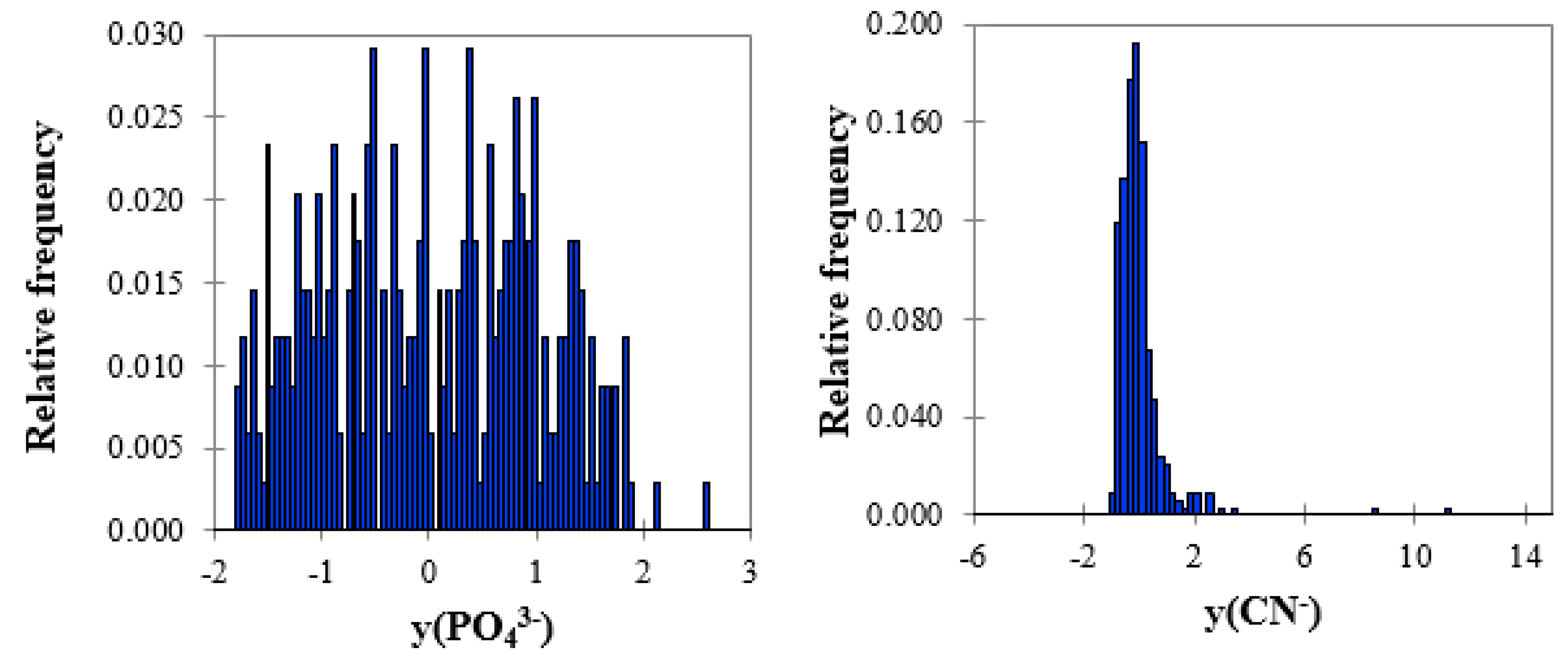
The raw wastewaters mixed from municipal and industrial ones were characterized by the 11 parameters listed in Table 1. The wastewater data were standardized as mentioned above: the original parameters xj were scaled and centred to obtain the transformed parameters yj which were further used by us to approximate their density functions pi,j by relative frequencies f(yi,j) to be used in Equation (2). Two examples of histograms with the highest (PO43−) and lowest entropy (CN−) are shown in Figure 1.
The entropy values summarized in Table 2 decreased in the sequence PO43− > NH4+ > TDS > TN > pH > BOD > COD > TSS > TP > phenol > CN−. Based on explanatory analysis, for example the P-P plot shown in Figure S1 (Supplementary Materials), the parameters were separated into two groups: the first group contained the parameters with higher entropy, such as PO43−, NH4+, TDS, TN, pH, BOD and COD, and the second one consisted of TSS, TP, phenol and CN− with lower entropy. It is obvious that entropy decreased with increasing kurtosis and skewness. The high values of kurtosis and skewness are typical for the variables, which changed in narrow intervals and existed in low magnitudes and, thus, their distributions were tailed. This is the case for the parameters in the second group.
The parameters of the first group were of higher entropy, that is, higher uncertainty, documented by the higher median absolute deviation (MAD) values. From a practical point of view, they should be monitored more frequently than the others by, for instance, the continual determination of pH, phosphate, ammonium, TN and COD. BOD and COD characterize mostly organic compounds, similar to TN and ammonium, which is the prevailing nitrogen form mostly resulting from hydrolysis of urea. Dissolved phosphate also enters wastewaters in the form of urea and detergents [41].
The parameters of the second group were of lower entropy, that is, lower uncertainty. Cyanide and phenol came from coke-making factories; their contractions were of 0.15–0.16 mg/L. The high kurtosis of TSS was caused by tailing of its distribution curve due to heterogeneity of wastewaters including sedimentation of solid particles during physico-chemical analyses.
3.2. Entropy Weighted Index
The calculated entropy weights were used by us to construct the entropy weighted index and to characterize the wastewater composition. A similar approach has been already used for the ground water quality assessment [26,27,31]. This is a simple way to describe complex water systems by one parameter. On the similar principle, for example, soil quality index (SQI) composed from several soil composition indicators (pH, TN, TP, cation exchange capacity, soil organic matter, etc.) has been successfully used for soil composition assessment [42,43]. An analogy with the SAW model, EWI was calculated for every sample i according to Equation (3). The difference 1-hj is called the relative redundancy and can be interpreted as a degree of diversification of information provided [15,16,18,25,30,44]. In information theory, the entropy weights represent useful information on variables (parameters). In other words, the higher the entropy weight, the more useful information on the parameter and vice versa.
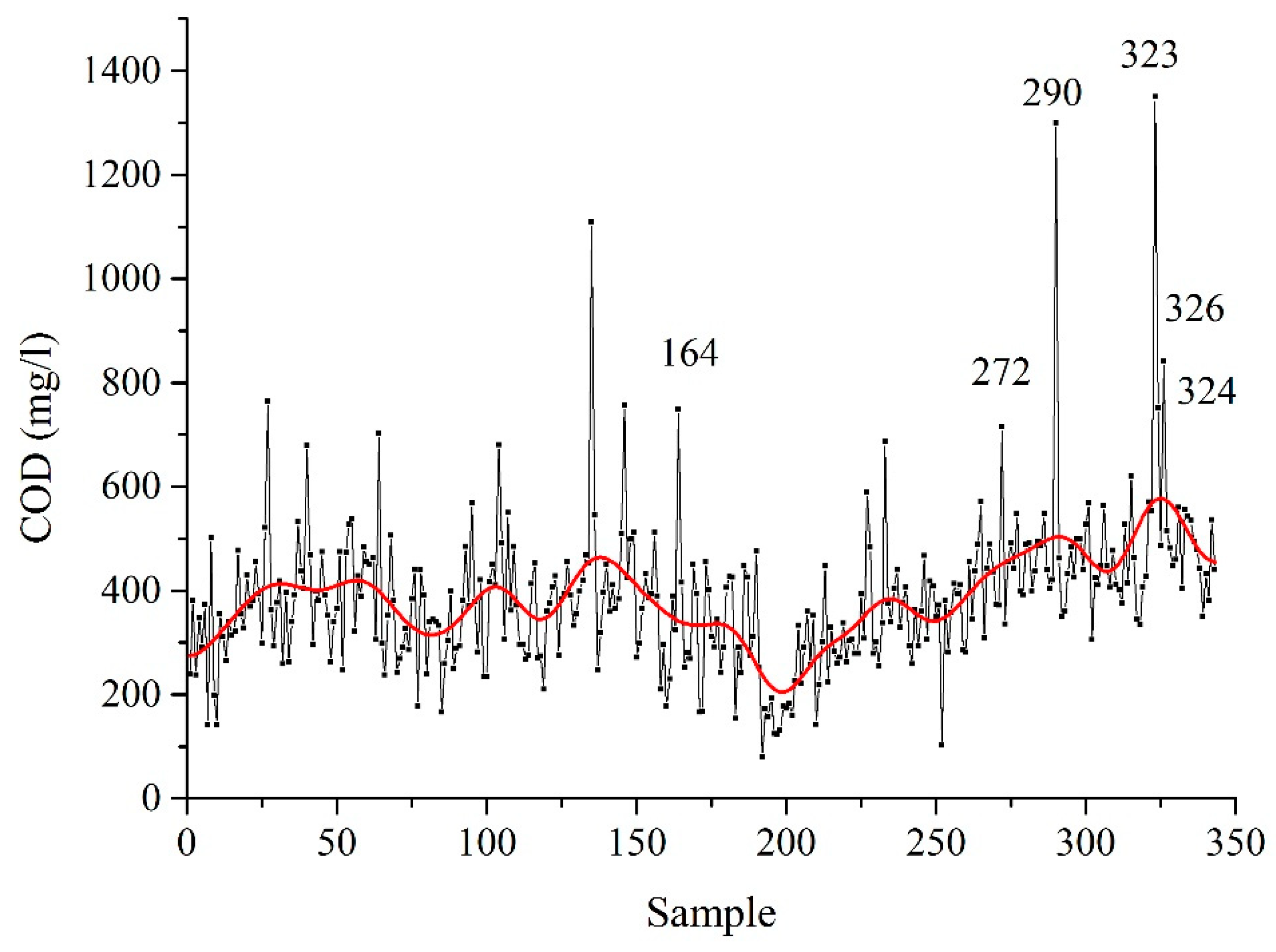
The EWI plot was constructed in order to demonstrate the temporal changes of wastewater composition during a year as shown in Figure 2. The samples were labeled according to their sequence of sampling, therefore the plot demonstrates their temporal composition changes. The EWI values were smoothed by the FFT algorithm by us to clearly see some trends in the data. In the first half of the year, the EWI values slightly increased during January and February and then oscillated around the mean (see the next paragraph) until a period between June and August. The minimal EWI value of 0.610 was reached at the end of July. In this period, people spend their time outside cities and production in some companies is reduced. In addition, higher temperatures accelerate chemical and biochemical processes in wastewaters. Conversely, during winter and autumn EWI increased due to the reduced migration of inhabitants and lower temperatures, which decelerated the chemical and biochemical processes in wastewaters. The EWI plot was compared with the plot of COD (Figure 3), which is the simple and typical wastewater parameter. Both plots were found to be similar as expected.
3.3. Statistical Analysis of EWI Data
The EWI values were statistically processed by exploratory analysis and outlaying samples corresponding to EWI ≥ 1.65 were identified: samples 38, 164, 272, 290, 302, 323, 324 and 326. The composition of the outliers is given in Table S1 (Supplementary Materials); the outlaying parameters detected by box-and-whisker plots were highlighted in bold. All the outliers were confirmed by means of the robust Mahalanobis distances calculated according to Equation (8). The cut-off limit was set at = 4.682 for the 97.5% quantile.
The outlaying samples were excluded from the dataset and remaining 335 were tested for normality which was proved by D’Agostino, Kolmogorov–Smirnov and moment tests (kurtosis = 3.403, skewness = −0.110). The EWI mean and standard deviation were calculated at 0.965 and 0.227, respectively; the EWI median was 0.972. The lower warning limit (LWL) and upper warning limit (UWL) were calculated at 0.511 and 1.419, respectively, and the lower control limit (LCL) and upper control limit (UCL) were calculated at 0.284 and 1.646, respectively (Figure 2). All these limits are commonly used for the statistical regulation of various processes and can be used for the regulation of the EWI values.
3.4. Verification of EWI
The principal component weighted index [32] was employed in order to verify the EWI data. RPCA was applied for this purpose. PCWI was defined as follows
where uk stands for the weight of k-th principal component calculated as
where λk is the eigenvalue of k-th PC and q is the number of selected principal components. The objectivity of PCWI is based on the following facts: (i) principal components are orthogonal and thus independent which is consistent with the SAW theory and (ii) the weights of principal components correspond to their eigenvalues expressing their importance. When all 11 principal components were used (q = 11) their weights were equal to their variabilities. The scree and cumulative plots are shown in Figure 4.
The significant linear correlation between EWI and PCWI (r = 0.910) is shown in Figure 5. It demonstrates a strong agreement between both indexes and confirms the validity of EWI. The outlaying samples (38, 164, 272, 290, 302, 323, 324 and 326) not included into the regression are also clearly visible. In addition, the scree plot indicated four main principal components and PCWI composed from them also correlated well with EWI: the correlation coefficient r = 0.900.
4. Conclusions
The wastewater composition was evaluated using the Shannon entropy. Entropy of the wastewater parameters calculated based on their histograms decreased in the order: PO43− > NH4+ > TDS > TN > pH > BOD > COD > TSS > TP > phenol > CN−. According to the entropy values the parameters were separated into two groups: (i) phosphate, ammonium, TDS, TN, pH, BOD and COD and (ii) TSS, TP, phenol and cyanide. The parameters from the first group should be monitored frequently because of their higher uncertainty in terms of the higher temporal changes.
The entropy weights were calculated by us to define the entropy weighted index analogous to the SAW model. The EWI plot showed the temporal changes of wastewater composition during one year. The EWI values were statistically analyzed by univariate statistics and the limits for statistical regulation, such as UCL, LCL, UWL and LWL, were calculated. In addition, the outlaying samples were detected by univariate and multivariate analyses. EWI was verified by comparison with PCWI composed from the robust principal components. EWI agreed well with PCWI which was documented with their correlation coefficient r = 0.910 for all principal components and r = 0.900 for four main ones.
The validation confirmed the capability of EWI to reliably characterize wastewater composition as the single indicator and could be of interest to BWWTP operators as well as other experts and decision makers in this field. The main advantage of EWI is the simple histogram-based calculation of entropy with no need of the normal distribution of the used parameters. Based on the results mentioned above one can conclude that information entropy is suitable for the evaluation of wastewater composition.
Supplementary Materials
The following are available online at https://www.mdpi.com/2073-4441/12/4/1095/s1, Figure S1: P-P plot of parameter entropies, Table S1: Composition of identified outlaying samples.
Funding
This work was financially supported by the projects “Institute of Environmental Technology—Excellent Research” (CZ.02.1.01/0.0/0.0/16_019/0000853) and Large Research Infrastructure ENREGAT (project No. LM 2018098) provided by the Ministry of Education, Youth and Sports of the Czech Republic. The author has no conflicts of interest to declare.
Conflicts of Interest
The author declares no conflicts of interest. The funders had no role in the design of the study; in the collection, analyses, or interpretation of data; in the writing of the manuscript, or in the decision to publish the results.
References
- Shannon, C.E. A mathematical theory of communication. Bell Syst. Tech. J. 1948, 27, 379–423. [Google Scholar] [CrossRef] [Green Version]
- Dang, T.K.L.; Meckbach, C.; Tacke, R.; Waack, S.; Gültas, M.A. Novel Sequence-Based Feature for the Identification of DNA-Binding Sites in Proteins Using Jensen–Shannon Divergence. Entropy 2016, 18, 13. [Google Scholar] [CrossRef] [Green Version]
- Maruyama, T.; Kawachi, T.; Singh, V.P. Entropy-based assessment and clustering of potential water resources availability. J. Hydrol. 2005, 309, 104–113. [Google Scholar] [CrossRef]
- Tsallis, C. Approach of Complexity in Nature: Entropic Nonuniqueness. Axioms 2016, 5, 20. [Google Scholar] [CrossRef] [Green Version]
- Chamberlin, R. The Big World of Nanothermodynamics. Entropy 2014, 17, 52–73. [Google Scholar] [CrossRef] [Green Version]
- Barigye, S.J.; Marrero-Ponce, Y.; Perez-Gimenez, F.; Bonchev, D. Trends in information theory-based chemical structure codification. Mol Divers 2014, 18, 673–686. [Google Scholar] [CrossRef]
- Eckschlager, K.; Štěpánek, V.; Danzer, K. A review of information theory in analytical chemometrics. J. Chemom. 1990, 4, 195–216. [Google Scholar] [CrossRef]
- Farhadinia, B. Information measures for hesitant fuzzy sets and interval-valued hesitant fuzzy sets. Inf. Sci. 2013, 240, 129–144. [Google Scholar] [CrossRef]
- Gültas, M.; Haubrock, M.; Tüysüz, N.; Waack, S. Coupled mutation finder: A new entropy-based method quantifying phylogenetic noise for the detection of compensatory mutations. BMC Bioinform. 2012, 13, 225. [Google Scholar] [CrossRef] [Green Version]
- Martin, L.C.; Gloor, G.B.; Dunn, S.D.; Wahl, L.M. Using information theory to search for co-evolving residues in proteins. Bioinformatics 2005, 21, 4116–4124. [Google Scholar] [CrossRef] [Green Version]
- Guido, R.C. A tutorial review on entropy-based handcrafted feature extraction for information fusion. Inf. Fusion 2018, 41, 161–175. [Google Scholar] [CrossRef]
- Oguz, I.; Cates, J.; Datar, M.; Paniagua, B.; Fletcher, T.; Vachet, C.; Styner, M.; Whitaker, R. Entropy-based particle correspondence for shape populations. Int. J. Comput. Assist. Radiol. Surg. 2016, 11, 1221–1232. [Google Scholar] [CrossRef] [PubMed]
- Ijadi Maghsoodi, A.; Abouhamzeh, G.; Khalilzadeh, M.; Zavadskas, E.K. Ranking and selecting the best performance appraisal method using the MULTIMOORA approach integrated Shannon’s entropy. Front. Bus. Res. China 2018, 12. [Google Scholar] [CrossRef] [Green Version]
- Tsallis, C. Economics and Finance: Q-Statistical Stylized Features Galore. Entropy 2017, 19, 457. [Google Scholar] [CrossRef] [Green Version]
- Wang, Q.; Wu, C.; Sun, Y. Evaluating corporate social responsibility of airlines using entropy weight and grey relation analysis. J. Air Transp. Manag. 2015, 42, 55–62. [Google Scholar] [CrossRef]
- Shemshadi, A.; Shirazi, H.; Toreihi, M.; Tarokh, M.J. A fuzzy VIKOR method for supplier selection based on entropy measure for objective weighting. Expert Syst. Appl. 2011, 38, 12160–12167. [Google Scholar] [CrossRef]
- Zhang, Y.; Yang, Z.; Li, W. Analyses of urban ecosystem based on information entropy. Ecol. Model. 2006, 197, 1–12. [Google Scholar] [CrossRef]
- Delgado, A.; Romero, I. Environmental conflict analysis using an integrated grey clustering and entropy-weight method: A case study of a mining project in Peru. Environ. Model. Softw. 2016, 77, 108–121. [Google Scholar] [CrossRef]
- Kawachi, T.; Maruyama, T.; Singh, V.P. Rainfall entropy for delineation of water resources zones in Japan. J. Hydrol. 2001, 246, 36–44. [Google Scholar] [CrossRef]
- Singh, V.P. Entropy Theory and its Application in Environmental and Water Engineering; John Wiley & Sons, Ltd.: Hoboken, NJ, USA, 2013; p. 642. [Google Scholar]
- Frank, B.; Pompe, B.; Schneider, U.; Hoyer, D. Permutation entropy improves fetal behavioural state classification based on heart rate analysis from biomagnetic recordings in near term fetuses. Med. Biol. Eng. Comput. 2006, 44, 179–187. [Google Scholar] [CrossRef]
- Güçlü, B. Maximizing the entropy of histogram bar heights to explore neural activity: A simulation study on auditory and tactile fibers. Acta Neurobiol. Exp. 2005, 65, 399–407. [Google Scholar]
- Hasson, U. The neurobiology of uncertainty: Implications for statistical learning. Philos. Trans. R. Soc. Lond. B Biol. Sci. 2017, 372. [Google Scholar] [CrossRef] [PubMed] [Green Version]
- Grupp, H. The concept of entropy in scientometrics and innovation research. Scientometrics 1990, 18, 219–239. [Google Scholar] [CrossRef]
- Zhang, Y.; Qian, Y.; Huang, Y.; Guo, Y.; Zhang, G.; Lu, J. An entropy-based indicator system for measuring the potential of patents in technological innovation: Rejecting moderation. Scientometrics 2017, 111, 1925–1946. [Google Scholar] [CrossRef]
- Islam, A.; Ahmed, N.; Bodrud-Doza, M.; Chu, R. Characterizing groundwater quality ranks for drinking purposes in Sylhet district, Bangladesh, using entropy method, spatial autocorrelation index, and geostatistics. Environ. Sci. Pollut. Res. Int. 2017, 24, 26350–26374. [Google Scholar] [CrossRef]
- Gorgij, A.D.; Kisi, O.; Moghaddam, A.A.; Taghipour, A. Groundwater quality ranking for drinking purposes, using the entropy method and the spatial autocorrelation index. Environ. Earth Sci. 2017, 76. [Google Scholar] [CrossRef]
- Shyu, G.S.; Cheng, B.Y.; Chiang, C.T.; Yao, P.H.; Chang, T.K. Applying factor analysis combined with kriging and information entropy theory for mapping and evaluating the stability of groundwater quality variation in Taiwan. Int. J. Environ. Res. Public Health 2011, 8, 1084–1109. [Google Scholar] [CrossRef]
- An, Y.; Zou, Z.; Li, R. Water quality assessment in the Harbin reach of the Songhuajiang River (China) based on a fuzzy rough set and an attribute recognition theoretical model. Int. J. Environ. Res. Public Health 2014, 11, 3507–3520. [Google Scholar] [CrossRef] [Green Version]
- Wu, J.; Li, P.; Qian, H.; Chen, J. On the sensitivity of entropy weight to sample statistics in assessing water quality: Statistical analysis based on large stochastic samples. Environ. Earth Sci. 2015, 74, 2185–2195. [Google Scholar] [CrossRef]
- Wu, J.; Peiyue, L.; Hui, Q. Groundwater Quality in Jingyuan County, a Semi-Humid Area in Northwest China. E J. Chem. 2011, 8. [Google Scholar] [CrossRef]
- Praus, P. Principal Component Weighted Index for Wastewater Quality Monitoring. Water 2019, 11, 2376. [Google Scholar] [CrossRef] [Green Version]
- Hwang, C.L.; Yoon, K. Multiple Attribute Decision Making; Springer: Berlin/Heidelberg, Germany, 1981; p. 269. [Google Scholar]
- Wold, S.; Esbensen, K.; Geladi, P. Principal component analysis. Chemom. Intell. Lab. Syst. 1987, 2, 37–52. [Google Scholar] [CrossRef]
- Praus, P. Water quality assessment using SVD-based principal component analysis of hydrological data. Water Sa 2005, 31, 417–422. [Google Scholar] [CrossRef] [Green Version]
- Praus, P. SVD-based principal component analysis of geochemical data. Cent. Eur. J. Chem. 2005, 3, 731–741. [Google Scholar] [CrossRef]
- Hubert, M.; Debruyne, M. Minimum covariance determinant. Comput. Stat. 2009, 2, 8. [Google Scholar] [CrossRef]
- Rousseeuw, P.J.; Driessen, K.V. A Fast Algorithm for the Minimum Covariance Determinant Estimator. Technometrics 1999, 41, 212–223. [Google Scholar] [CrossRef]
- Hubert, M.; Rousseeuw, P.J.; Vanden Branden, K. ROBPCA: A New Approach to Robust Principal Component Analysis. Technometrics 2005, 47, 64–79. [Google Scholar] [CrossRef]
- Verboven, S.; Hubert, M. LIBRA: A MATLAB library for robust analysis. Chemom. Intell. Lab. Syst. 2005, 75, 127–136. [Google Scholar] [CrossRef]
- Yeoman, S.; Stephenson, T.; Lester, J.N.; Perry, R. The removal of phosphorus during wastewater treatment. A review. Environ. Pollut. 1988, 49, 183–233. [Google Scholar] [CrossRef]
- Yu, P.; Liu, S.; Zhang, L.; Li, Q.; Zhou, D. Selecting the minimum data set and quantitative soil quality indexing of alkaline soils under different land uses in northeastern China. Sci. Total Environ. 2018, 616, 564–571. [Google Scholar] [CrossRef]
- Li, P.; Zhang, T.; Wang, X.; Yu, D. Development of biological soil quality indicator system for subtropical China. Soil Tillage Res. 2013, 126, 112–118. [Google Scholar] [CrossRef]
- Lotfi, F.H.; Fallahnejad, R. Imprecise Shannon’s Entropy and Multi Attribute Decision Making. Entropy 2010, 12, 53–62. [Google Scholar] [CrossRef] [Green Version]
Figure 1.
Histograms of phosphate and cyanide.

Figure 2.
Entropy weighted index (EWI) plot of wastewaters during year. The labels identify the samples.
Figure 2.
Entropy weighted index (EWI) plot of wastewaters during year. The labels identify the samples.

Figure 3.
Chemical oxygen demand (COD) plot of wastewaters during year. The labels identify the samples.
Figure 3.
Chemical oxygen demand (COD) plot of wastewaters during year. The labels identify the samples.

Figure 4.
Cumulative and scree plots of principal components.

Figure 5.
Linear regression between principal component weighted index (PCWI) and EWI.


Table 1.
Summary statistics of wastewater composition.
| Param. | Mean | Median | St. Dev. | MAD | Min. | Max. | Skew. | Kurt. |
|---|---|---|---|---|---|---|---|---|
| NH4+ | 35.5 | 36.1 | 10.7 | 8.90 | 5.56 | 68.9 | −0.033 | 3.42 |
| BOD | 194 | 191 | 70.6 | 54.9 | 25.7 | 625 | 1.25 | 8.79 |
| COD | 387 | 381 | 144 | 113 | 80.1 | 1350 | 2.14 | 14.2 |
| Phenol | 0.18 | 0.16 | 0.14 | 0.059 | 0.02 | 1.57 | 4.93 | 40.1 |
| PO43− | 5.22 | 5.13 | 2.63 | 3.32 | 0.526 | 12.1 | 0.044 | 1.97 |
| CN− | 0.174 | 0.146 | 0.165 | 0.0786 | 0.016 | 2.03 | 6.40 | 63.2 |
| TN | 40.0 | 40.8 | 9.30 | 7.41 | 13.2 | 90 | 0.050 | 5.52 |
| TSS | 280 | 256 | 141 | 94.9 | 44 | 1665 | 3.61 | 31.0 |
| TP | 6.26 | 6.25 | 2.54 | 1.39 | 1.40 | 34.7 | 5.06 | 52.4 |
| pH | 7.74 | 7.75 | 0.188 | 0.178 | 6.89 | 8.22 | −0.623 | 5.21 |
| TDS | 706 | 730 | 129 | 91.9 | 276 | 1088 | −0.856 | 4.32 |
Note: MAD is median absolute deviation. Except for pH, the units of all parameters were mg/L.
Table 2.
Entropy and entropy weights of wastewater parameters.
| Parameter | Entropy | Entropy Weight |
|---|---|---|
| PO43− | 4.196 | 0.0282 |
| NH4+ | 3.999 | 0.0417 |
| TDS | 3.801 | 0.0554 |
| TN | 3.695 | 0.0628 |
| pH | 3.653 | 0.0656 |
| BOD | 3.573 | 0.0712 |
| COD | 3.456 | 0.0793 |
| TSS | 2.647 | 0.135 |
| TP | 2.497 | 0.1453 |
| Phenol | 2.384 | 0.1531 |
| CN− | 2.250 | 0.1624 |
© 2020 by the author. Licensee MDPI, Basel, Switzerland. This article is an open access article distributed under the terms and conditions of the Creative Commons Attribution (CC BY) license (http://creativecommons.org/licenses/by/4.0/).
Share and Cite
MDPI and ACS Style
Praus, P. Information Entropy for Evaluation of Wastewater Composition. Water 2020, 12, 1095. https://doi.org/10.3390/w12041095
AMA Style
Praus P. Information Entropy for Evaluation of Wastewater Composition. Water. 2020; 12(4):1095. https://doi.org/10.3390/w12041095
Chicago/Turabian StylePraus, Petr. 2020. "Information Entropy for Evaluation of Wastewater Composition" Water 12, no. 4: 1095. https://doi.org/10.3390/w12041095
Note that from the first issue of 2016, this journal uses article numbers instead of page numbers. See further details here.