Lag Times as Indicators of Hydrological Mechanisms Responsible for NO₃-N Flushing in a Forested Headwater Catchment

Abstract

Understanding the temporal variability of the nutrient transport from catchments is essential for planning nutrient loss reduction measures related to land use and climate change. Moreover, observations and analysis of nutrient dynamics in streams draining undisturbed catchments are known to represent a reference point by which human-influenced catchments can be compared. In this paper, temporal dynamics of nitrate-nitrogen (NO₃-N) flux are investigated on an event basis by analysing observed lag times between data series. More specifically, we studied lag times between the centres of mass of six hydrological and biogeochemical variables, namely discharge, soil moisture at three depths, NO₃-N flux, and the precipitation hyetograph centre of mass. Data obtained by high-frequency measurements (20 min time step) from 29 events were analysed. Linear regression and multiple linear regression (MLR) were used to identify relationships between lag times of the above-mentioned processes. We found that discharge lag time (LAG_Q) and NO₃-N flux lag time (LAG_N) are highly correlated indicating similar temporal response to rainfall. Moreover, relatively high correlation between LAG_N and soil moisture lag times was also detected. The MLR model showed that the most descriptive variable for both LAG_N and LAG_Q is amount of precipitation. For LAG_N, the change of the soil moisture in the upper two layers was also significant, suggesting that the lag times indicate the primarily role of the forest soils as the main source of the NO₃-N flux, whereas the precipitation amount and the runoff formation through the forest soils are the main controlling mechanisms.

1. Introduction

Human-induced land use changes and climate change have raised a number of questions related to their impacts on runoff generation, soil erosion, and nutrient cycle [1,2]. Therefore, nutrients, especially nitrogen, due to its essential role for all living things, and it’s most soluble and mobile form, nitrate (NO₃), have been the subject of many hydrological and biogeochemical studies [3,4,5]. Rainfall events impact on the changes in the amount of nitrate-nitrogen (NO₃-N) in the stream water in two ways [6]. Firstly, the rainwater itself contains a certain amount of NO₃-N. Secondly, rainwater represents a transport medium and hydrological driver by which additional quantities of NO₃-N are mobilized from other sources (e.g., from soil, litter). In headwater catchments, which respond relatively quickly to rainfall events (precipitation–discharge lag time ranges from hours to a few minutes in case of micro catchments), high-frequency measurements are needed to capture these changes [7,8,9], and to describe and quantify hydrological and biogeochemical processes [10]. However, to assess different impacts on the nitrogen cycle, monitoring and observations from natural and undisturbed areas, i.e., covered by natural vegetation and with no or low population density, are needed to represent crucial information on the baseline conditions [11,12].

One of the most frequently applied methods to evaluate the causes and control mechanisms of changes in the water chemistry is analysis of the concentration–discharge (C–Q) relationship. For example, Musolff et al. [13] used monthly to bi-monthly concentration and discharge data from nine catchments in Germany to determine the solute export regimes based on the catchment properties. Duncan et al. [9] compared C–Q patterns obtained by high-frequency monitoring and weekly grabbed samples and found that from low-frequency data, only seasonal patterns can be observed, while high-frequency data are needed to reveal complex hydrological and biogeochemical interactions. Moreover, there are many studies where different indices were developed and applied based on the bivariate diagrams of hysteresis loops to describe the relationship between the response (dependent) variable (C) and the independent variable (Q) (e.g., References [14,15,16]). Presence of hysteresis loop is a consequence of the time lag between the variables [17]. In this way, lag time between NO₃-N concentration and discharge [14,18] and soil moisture and discharge [16] have been investigated. Some studies addressed the time lags between C and Q only in qualitative terms [19,20]. However, to the authors’ knowledge, there is no research that would comprehensively address lag times of processes that affect the dynamics of NO₃-N flushing along main rainfall runoff pathways, namely from precipitation, subsurface flow (soil moisture), and surface runoff (stream discharge). Therefore, the present study aims to address lag times between the aforementioned processes taking into account the flux of NO₃-N instead of concentration, as is the practice in numerous other studies. In this way, more representative information regarding the temporal mass dynamics of NO₃-N is obtained, since discharge can account for much of the variability in solute concentrations [21]. Discharge is usually estimated based on the water level, which has been found to be able to fluctuate for some centimetres in headwater streams due to the reasons stemming from the amount of solar energy reaching the hyphoreic zone (e.g., precipitation, evapotranspiration, changes in hydraulic gradient) [22] and consequently influence both the discharge and solute concentration in the stream. Moreover, hydrograph and chemograph can consequently result in multiple peaks, meaning that selection of the representative peak can be a challenge, especially where time-to-peak is in question. The same concept was used in the study of Banasik et al. [23], where sediment load time lags were addressed. They found that the time lag of the sediment load is shorter than that of the discharge and that there is a strong linear correlation between them. A similar temporal dynamic was also found by Bezak et al. [24], who made their conclusions based on diagrams’ peaks.

The aim of this study is three-fold. First, the lag times as the difference between the time of occurrence of precipitation hyetograph centre of mass and centres of mass of other hydrological variables, namely discharge, NO₃-N flux, and volumetric soil moisture in three depths, are calculated. Secondly, individual lag times are analysed in order to characterise time distribution of hydrological processes in small, highly responsive, undisturbed headwater catchment. Thirdly, the results are discussed in terms of the interdependence of the processes with respect to the known catchment hydrological characteristics. The results of this study contribute to improved understanding of complex, hydrologically induced processes of nitrogen flushing and export from catchments.

2. Materials and Methods

2.1. Study Area

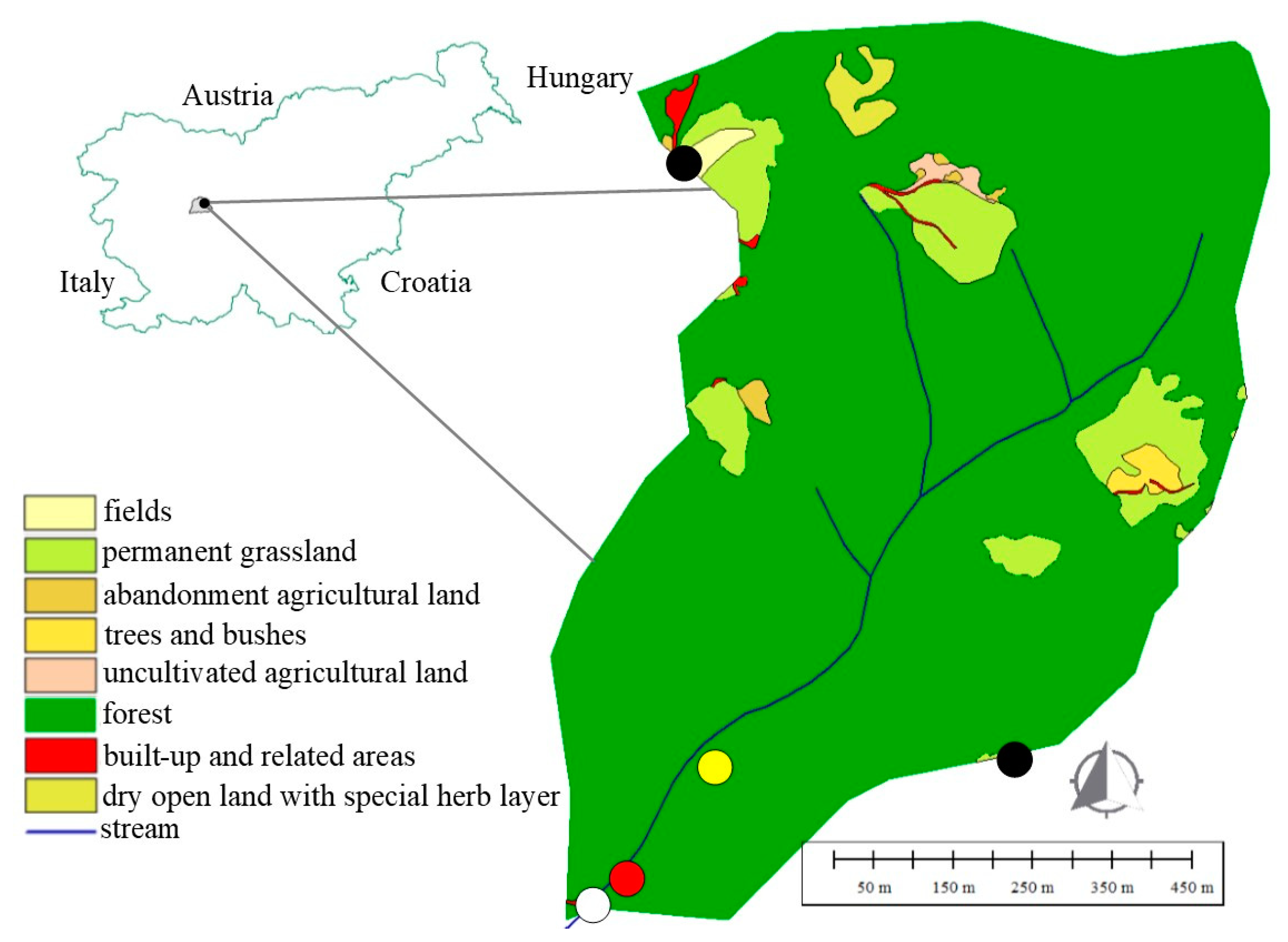
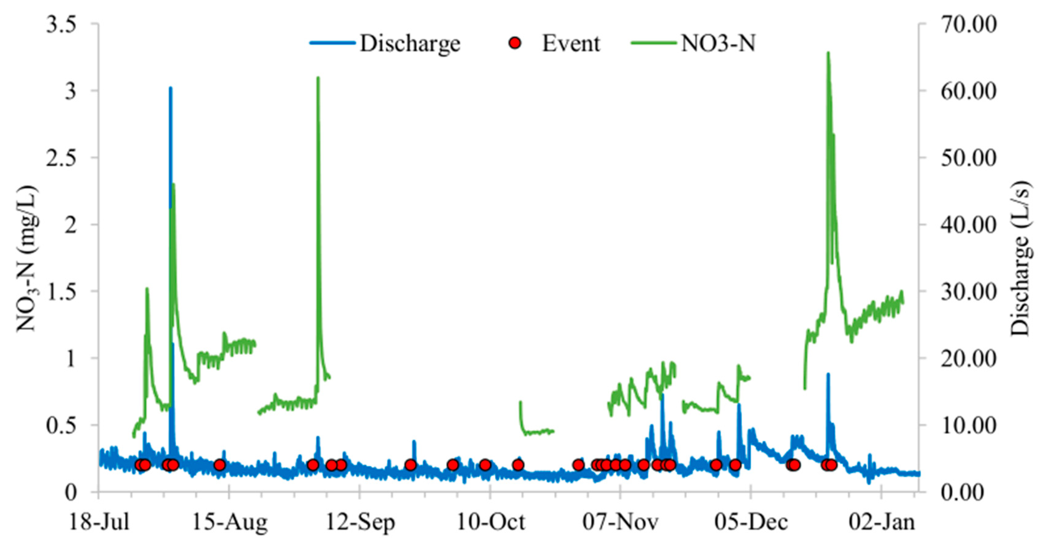
The Kuzlovec torrential stream is part of the larger Gradaščica river catchment, which is one of the major tributaries of the Ljubljanica river, Slovenia (Figure 1). The stream is 1.3 km long with an average slope of 22.2%. The catchment area of the Kuzlovec stream is 0.71 km² with an average slope of 51.6% and maximum slopes up to 105% [25]. For such small torrential catchments, the time of concentration is usually estimated to be short (in the range of 1–2 h) [26]. From the observed hydrographs, we can see that the falling limb of the hydrograph is also very steep, the discharge falls to pre-event values soon after the rainfall events end (in a couple of hours), as can be seen from Figure 2.

Dominant land use is forest (90%) with about the same proportion of mixed and deciduous forest (Figure 1). The next major land use is permanent grassland (7%). Other natural vegetation, namely abandonment agricultural land, trees and bushes, uncultivated agricultural land, and fields, covers the rest of the catchment (2.5%). 0.5% of the catchment represents built-up areas related to the presence of unpaved forest roads. The dominant soil is rendzina on limestone and dolomite with relatively high erodibility [25]. A detailed soil survey was conducted at the location of soil moisture measurements. Nitrogen availability decreases with soil depth, namely from 23 mg/L NO₃-N in the 0–4 cm layer to 1.3 mg/L NO₃-N in the 55–90 cm layer. The carbon-to-nitrogen ratio (C/N) varies through soil depths, with the lowest ratio 12.6 in the two middle layers and with the highest ratio 24.5 in the deepest layer. The soil is classified as well permeable (2–3 × 10⁻² cm/s) and rarely saturated. The average annual precipitation is between 1600 and 1800 mm, with long-term (2000–2019) average monthly maximums in November and minimums in January. Mean monthly temperatures vary between 18.1 and 19.8 °C in the summer months, and between 0.1 and 1.3 °C in the winter months [27].

2.2. Measurements and Data

In the scope of this study, 29 rainfall-runoff events were measured that occurred between 18 July 2019 and 10 January 2020 (Figure 2, red dots). The rainfall events with more than 10 mm of cumulative precipitation were taken into account. The start of the event was set as the time of the beginning of the rainfall, as it was done also in Bezak et al. [28]. To determine the end of the event or the separation point between the two events, we considered the criterion that there is no precipitation for at least four hours between the two events. The methodology of screening the hydrographs was used to determine the time between two consecutive events (e.g., Reference [28]). Guo [29] suggests that the time between events is equal to or longer than the time of concentration. According to Adams and Papa [30], a shorter inter-event time is more appropriate for smaller catchments with a quick response time. We found that most of the hydrographs reach the approximate pre-event discharge after 4 h of the last recorded precipitation data, which is more than two times the estimated time of concentration. Moreover, a longer inter-event time would lead to problems with multiple-peak hydrographs and merging consecutive events into one event. Baseflow was not excluded from the total runoff. As can be seen from Figure 2, the baseflow is relatively constant. Consequently, we believe baseflow has a limited effect on the lag-time calculations (e.g., if methods similar to constant monthly baseflow values were used [31]).

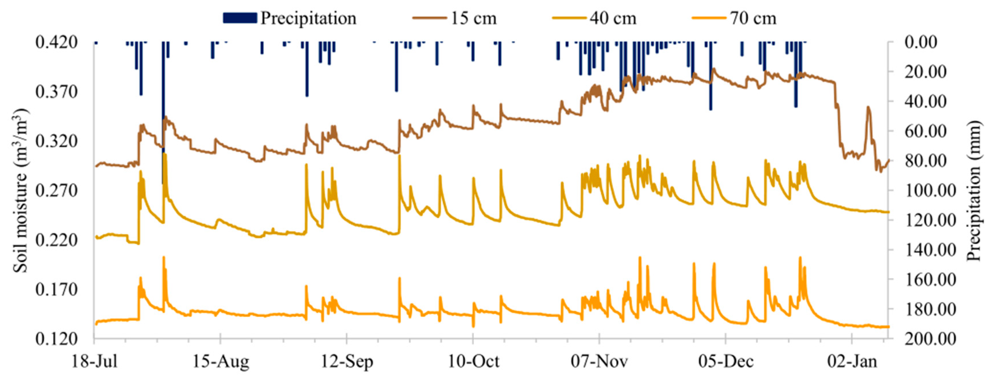
Water level data were measured at 10 min resolution (HOBO Fresh Water Level Data Logger), which were converted to discharge data using the rating curve. Data loggers measure hydrostatic and barometric pressure above the sensor located in the logger (i.e., absolute pressure). Therefore, to obtain the water level, data that are recorded with a logger installed in the water are compensated for barometric pressure measured with an additional data logger that is installed on the ground in the immediate vicinity. A stage–discharge relationship (i.e., rating curve) was determined by performing discharge measurements during contrasting hydrological conditions (i.e., low- and high-flows). Discharge data were aggregated to 20 min intervals to match the measurement frequency of other variables. Tipping-bucket rain gauges (HOBO RG3-M) were used for recording precipitation. Multiparameter sonde (Hydrolab MS5) was used for measurements of stream water chemistry, i.e., nitrate concentration, pH, temperature, and electrical conductivity. A drift correction approach was performed approximately biweekly by taking samples in the field which were later analysed in the laboratory. Soil moisture was measured continuously at 20 min time resolution by volumetric water content sensors (m³/m³) (ECH2O 5TM) at three depths, namely 15, 40, and 70 cm (Figure 3).

The precipitation amount of 29 events varied between 10.2 and 60.3 mm, while rainfall duration ranged between 40 min and 25 h. The highest monitored discharge was 60.3 L/s (

Table 1. General information about 29 rainfall events. P_duration and P_amount are duration and amount of rianfall, respectively, I_mean and I_max are mean and average rainfall intensity, respectively, Q_max and C_max are the maximum discharge and NO₃-N concentration respectively, ΔQ and ΔC are range of discharge and NO₃-N concentration respectively, SM15, SM40, and SM70 are the average soil moisture values in m³/m³ at 15, 40, and 70 cm, respectively. ΔQ and ΔC are calculated as the difference between maximum and minimum value of the individual event.

Event	Pduration (min)	Pamount (mm)	Imean (mm/min)	Imax (mm/min)	Qmax (L/s)	ΔQ (L/s)	Cmax (mg/L)	ΔC (mg/L)	SM15	SM40	SM70
1	180	15	0.083	0.6	8.76	5.15	1.17	0.62	0.31	0.25	0.16
2	1100	35.7	0.032	0.33	7.18	3.12	1.52	0.81	0.33	0.27	0.17
3	200	60.3	0.302	1.425	60.27	55.97	2.11	1.47	0.33	0.27	0.17
4	240	35.7	0.149	0.495	22.01	16.79	2.30	1.06	0.34	0.28	0.17
5	40	10.2	0.255	0.405	6.64	3.04	1.45	0.12	0.34	0.26	0.15
6	560	11.55	0.021	0.21	5.98	3.65	1.19	0.17	0.32	0.24	0.15
7	380	34.2	0.090	0.315	8.14	4.42	3.08	2.33	0.33	0.26	0.16
8	200	13.5	0.068	0.135	3.94	1.53	-	-	0.32	0.26	0.16
9	540	14.7	0.027	0.255	5.82	3.49	-	-	0.33	0.27	0.15
10	300	30.9	0.103	0.405	7.55	5.51	-	-	0.32	0.26	0.16
11	460	15.45	0.034	0.09	4.95	2.77	-	-	0.35	0.27	0.15
12	480	15.6	0.033	0.09	4.55	2.06	-	-	0.34	0.26	0.14
13	140	15.9	0.114	0.255	5.09	2.91	-	-	0.35	0.27	0.15
14	900	12	0.013	0.06	4.95	2.62	-	-	0.35	0.25	0.14
15	840	14.7	0.018	0.09	3.20	1.23	-	-	0.36	0.27	0.15
16	1180	15.9	0.013	0.075	5.37	2.72	-	-	0.37	0.28	0.16
17	860	16.5	0.019	0.06	4.68	2.71	0.75	0.18	0.37	0.28	0.16
18	1040	15.9	0.015	0.06	5.52	2.95	0.81	0.15	0.37	0.28	0.16
19	980	24.9	0.025	0.225	5.37	2.80	0.85	0.28	0.37	0.28	0.16
20	2400	63	0.026	0.15	9.88	7.70	0.92	0.29	0.38	0.29	0.16
21	1160	44.4	0.038	0.315	14.53	11.43	0.97	0.28	0.38	0.29	0.16
22	660	12	0.018	0.09	6.31	2.48	0.86	0.08	0.38	0.28	0.16
23	800	33.6	0.042	0.165	10.36	4.37	0.97	0.16	0.38	0.29	0.17
24	920	36.3	0.039	0.165	8.97	6.64	0.82	0.23	0.38	0.28	0.16
25	1520	49.2	0.032	0.12	13.02	10.69	0.94	0.27	0.39	0.28	0.16
26	460	15.6	0.034	0.195	8.34	2.03	-	-	0.39	0.29	0.18
27	220	18.6	0.085	0.15	7.94	1.47	-	-	0.39	0.29	0.17
28	860	43.5	0.051	0.165	17.60	12.79	3.28	1.76	0.39	0.29	0.18
29	740	24.3	0.033	0.165	10.11	3.81	2.71	1.00	0.39	0.29	0.17

). However, average and minimum discharge during this period were 3.8 (±1.6) and 1.3 L/s, respectively. The range of NO₃-N concentration during 18 events was 0.41–3.28 mg/L, with an average value of 0.91 (±0.39) mg/L. Volumetric water content decreases with depth. Average values of soil moisture, monitored during the study, were 0.340 (±0.03), 0.250 (±0.02), and 0.147 (±0.01) m³/m³ at 15, 40, and 70 cm, respectively.

The dataset was split into 29 individual events starting with the first recorded precipitation. The events ended four hours after the last recorded precipitation data. For all 29 events, precipitation, discharge, and soil moisture data are available, while due to operational conditions (calibration of the sensors) and some technical problems, water chemistry data are available for only 18 events (Figure 2, Table 1).

2.3. Data Analysis

To estimate the lag times for rainfall-runoff-NO₃-N flux, we used the analogous methodology proposed by Banasik et al. [23] for estimation of sediment yield lag time and also applied by Hejduk et al. [32] for snowmelt events:

LAG_Q = M_Q − M_P

(1)

LAG_N = M_N − M_P

(2)

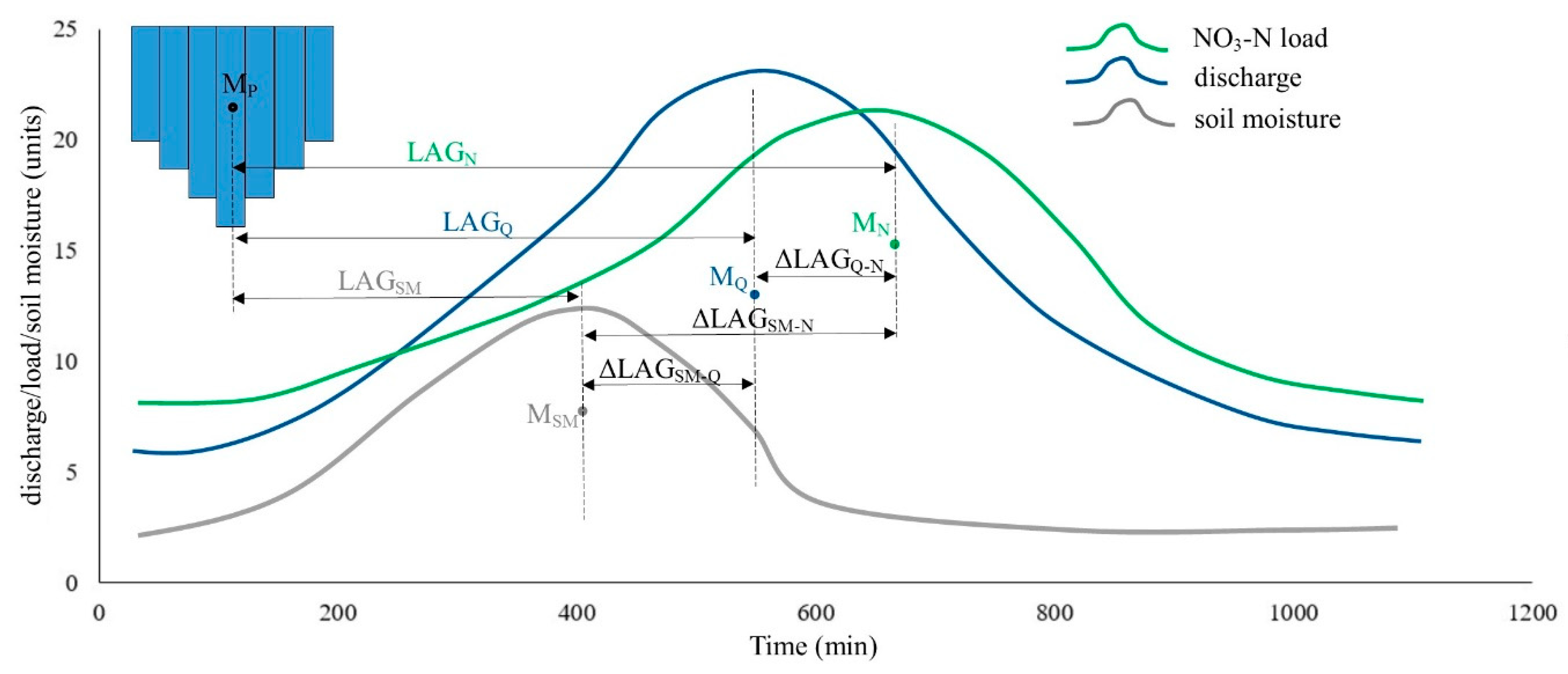
where LAG_Q is the river catchment lag time related to discharge, LAG_N is the lag time for the nitrate nitrogen flux, and M_Q, M_P, and M_N, are the first statistical moments (centres of mass) of the direct hydrograph, rainfall, and NO₃-N flux, respectively. LAG_Q and LAG_N represent the time from the precipitation hyetograph centroid to the time that half of the total runoff volume and NO₃-N mass have passed the measuring point, respectively. Since soil is the second input source of NO₃-N to the stream water, the lag times of centres of mass of volumetric soil moisture in three depth layers (M_SM15, M_SM40, M_SM70) were evaluated and compared with LAG_Q and LAG_N:

LAG_SM15 = M_SM15 − M_P

(3)

LAG_SM40 = M_SM40 − M_P

(4)

LAG_SM70 = M_SM70 − M_P

(5)

A schematic representation of individual lag times used in this paper is shown in Figure 4. The general equation for calculation of the first statistical moment (M_X) for discharge, NO₃-N load, and soil moisture is:

$$M_X=\frac{{\sum }_{i=1}^n\left(Y_i·t_i\right)}{{\sum }_{i=1}^n{Y}_i}$$

(6)

where Y_i is the amount of rainfall, NO₃-N flux, discharge, and soil moisture for i = 1, 2, …, n time periods of equal length. In Equation (6), t is the time from the beginning of the event to halfway through period i. In case of a 20 min time resolution of data, t = 10, 30, 50 … (n × 20 − 10). For example, let us assume we have a rainfall event with a duration of 60 min, where in the first 20 min we have 2 mm of rain, in the second 20 min 5 mm, and in the third 20 min 3 mm (i.e., the time step of measurements is 20 min). Therefore, in this case, the centroid is located 32 min after the start of the event.

To investigate the relations between the variables, i.e., runoff and NO₃-N flux, soil moisture and NO₃-N flux, and runoff and soil moisture, regression analysis was performed. Detailed analysis revealed that the results of two events might not be representative due to the duration of the event. According to our chosen criterion, these two events lasted more than 1 day. Nevertheless, we noticed that the rainfall stopped a few times and started again, but the dry period did not exceed 4 h. Intermediate dry periods may significantly influence the runoff formation in soils and the soil moisture and consequently, the lag times, therefore we excluded these two events from linear regression analysis.

Multiple linear regression (MLR) was used to model the relationship between dependent variables (P_duration, P_amount, I_mean, I_max, ΔC, ΔQ, C_max, Q_max, ΔSM15, SM15_max, ΔSM40, SM40_max, ΔSM70, SM70_max) (

Table 2. Dependent variables taken into account to model LAG_N (NO₃-N flux lag time) and LAG_Q (discharge lag time) using multiple linear regression.

Variable	Description	Units
Pduration	duration of rainfall	min
Pamount	amount of rainfall	mm
Imean	mean intensity	mm/min
Imax	maximum intensity	mm/min
ΔC	difference between max and min NO3-N concentration during the event	mg/L
Cmax	maximum concentration of NO3-N	mg/L
ΔQ	difference between maximum and minimum stream discharge during the event	L/s
Qmax	maximum stream discharge	L/s
ΔSM15	difference between maximum and minimum soil water content in 15 cm depth layer	m3/m3
ΔSM40	difference between maximum and minimum soil water content in 40 cm depth layer	m3/m3
ΔSM70	difference between maximum and minimum soil water content in 70 cm depth layer	m3/m3

) and the independent variable (LAG_N), and with the aim to identify the causes for the variation in NO₃-N lag time. The same dependent variables were used in the MLR to model LAG_Q. Therefore, by MLR, LAG_N, and LAG_Q are estimated as a linear function of predictors X₁, … X_J (corresponding to J dependent variables):

$$LAG=a_0+{\displaystyle \sum }_{i=1}^J{a}_i·X_i$$

(7)

where a₀, … a_J are the linear coefficients for the multiple linear regression estimated by using the least square method. Multiple linear regression was performed in R software [33] using the lm() function. For each of the linear coefficients, the following values are given as a result: standard error, t-value (estimate of coefficient divided by standard error), and p-value. Moreover, the multiple R² of the model indicates how much of the variance is explained by predictor variables (overall fit of the model). The multiple R² would increase by including more and more dependent variables, not necessarily improving the model performance (overfitting). Therefore, a joint report of multiple R² with adjusted R² is needed to more objectively evaluate the model. Unlike as in the case of multiple R², adjusted R² would decrease, if new included variables would not improve the model performance.

3. Results and Discussion

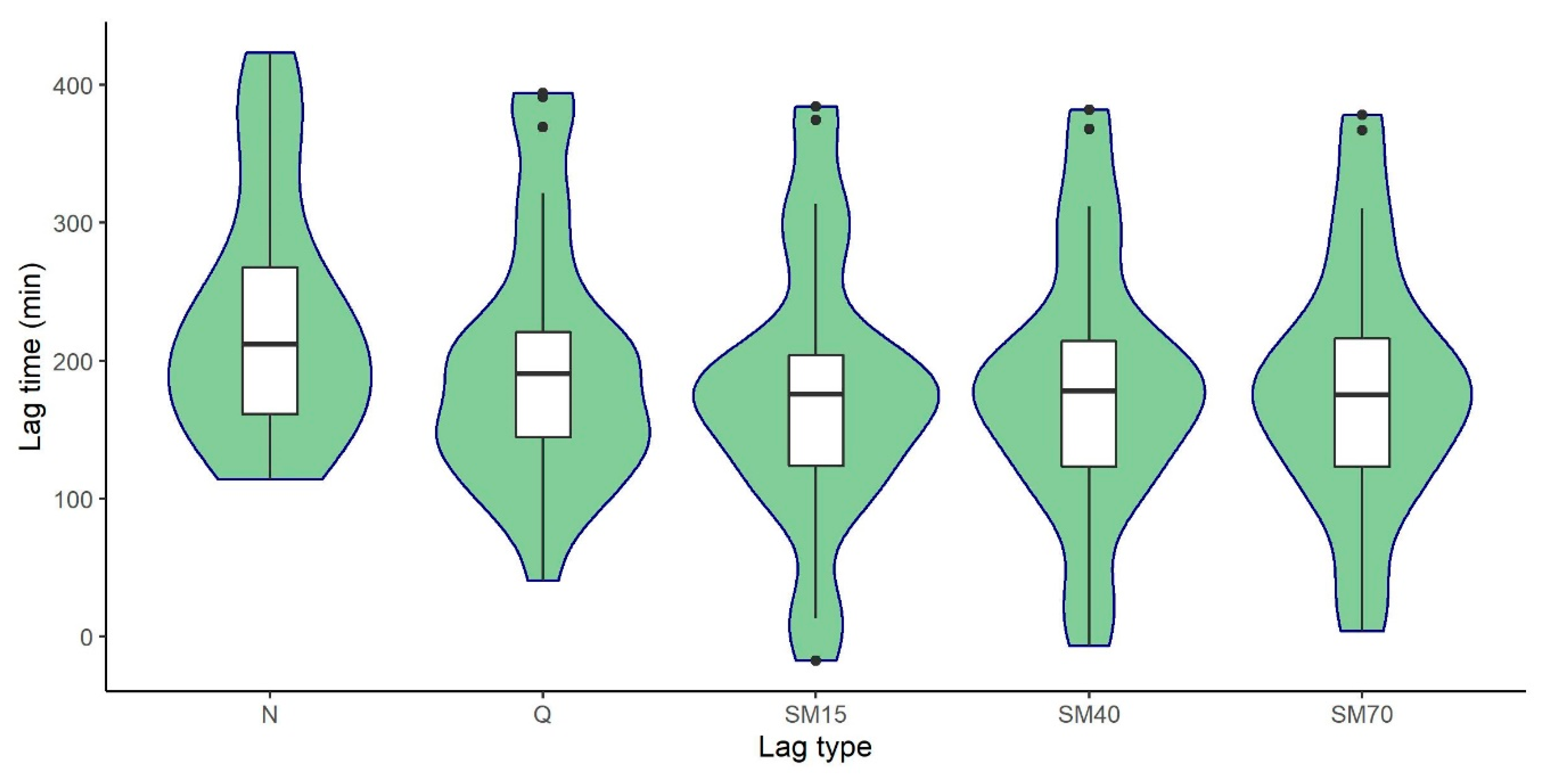
Centres of mass for six hydrological and biogeochemical variables from 29 events (July 2019–January 2020) were calculated to evaluate lag times, namely discharge lag time (LAG_Q), NO₃-N flux lag time (LAG_N), and soil moisture time lag (LAG_SM15, LAG_SM40, LAG_SM70) (Figure 5). LAG_Q and LAG_N for all events were positive, meaning that discharge and NO₃-N flux centres of mass (M_Q and M_N) occurred after the rainfall centre of mass. In other words, more than half of the rainfall had to fall to cause more than half of the runoff volume and NO₃-N mass to pass the measuring point in the Kuzlovec catchment. On average, M_Q and M_N occurred 3.2 and 3.6 h after M_P, respectively. Lag times of soil moisture are also mostly positive, however, there was one event with slightly negative LAG_SM15 that could be a consequence of antecedent precipitation (catchment wetness) conditions. M_SM15, M_SM40, and M_SM70 occurred almost simultaneously in the span of few minutes, confirming relatively fast water percolation through the soil horizons. On average, the centres of water content at all soil depths occurred 3.1 h after M_P.

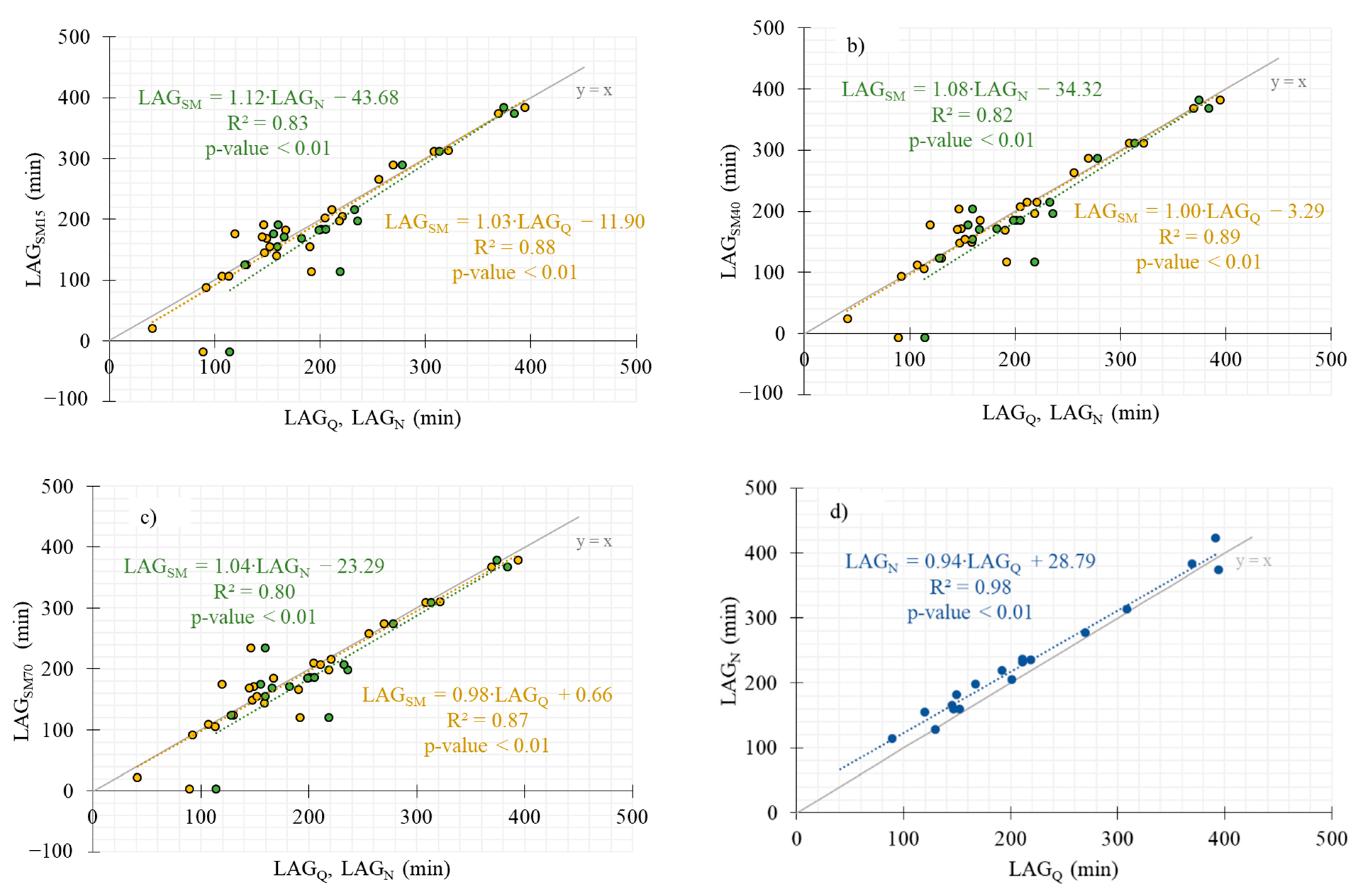
For further investigation of the relationships between observed rainfall-runoff formation processes and stream water nitrate fluxes, linear regression was performed. All pairs of soil moisture lag times (LAG_SM15, LAG_SM40, and LAG_SM70) and LAG_N and LAG_Q were analysed (Figure 6a–c). A statistically significant (p-value < 0.01) positive dependence between the variables at all three depths was found with coefficient of determination ranging between 0.80 and 0.89. All trend lines, representing the linear relationship between lag times of soil moisture and lag times of nitrogen flux (green dashed lines), are below the identity line (x = y). This means that centre of mass of soil moisture occurs before the centre of mass of NO₃-N flux. Moreover, together with a relatively high correlation coefficient, it can be assumed that soil water is a source of NO₃-N, identified in the stream after the rainfall event. A similar conclusion can also be made for the relationship between LAG_SM in all depths and LAG_Q. However, trend lines (orange dashed lines) are slightly below the identity line, almost overlapping it. The linear regression between LAG_N and LAG_Q (Figure 6d) revealed even stronger, statistically significant (p-value < 0.01) positive dependence with coefficient of determination 0.98. In this case, the trend line (blue dashed line) is above the identity line. Moreover, we analysed the relationship between the discharges and concentrations of NO₃-N by performing linear regression between the variables for each of the 18 events. We found that correlation coefficients vary between −0.68 and 0.93, with an average correlation coefficient 0.16. Seven out of eight events with a negative correlation occurred during the summer and early autumn seasons, indicating dilution of NO₃-N, while all 10 events with a positive correlation coefficient occurred during late autumn and winter seasons, indicating flushing of NO₃-N. The same export regimes were determined based on the slope between log(Q) and log(C), a methodology that is widely used for evaluating the dynamics of solute export from catchments (e.g., Reference [13]). During the summer and early autumn, the slope was negative (dilution), whereas during late autumn and winter, the slope was positive (flushing). This indicates that regardless of the seasonal variability of export regimes, the catchment behaviour shown through lag times is relatively consistent.

Results of multiple linear regression analysis showed that in case of LAG_N and LAG_Q, 92% and 91% of variance is explained by the models, respectively (

Table 3. Coefficients of the multiple linear regression (MLR) models for NO₃-N flux lag time (LAG_N) and discharge lag time (LAG_Q) taking into account 11 dependent variables: duration of rainfall (P_duration), rainfall amount (P_amount), mean rainfall intensity (I_mean), maximum rainfall intensity (I_max), difference between max and min NO₃-N concentration during the event (ΔC), maximum NO₃-N concentration (C_max), difference between max and min discharge during the event (ΔQ), maximum discharge (Q_max), differences between maximum and minimum soil water content in 15, 40, and 70 cm depth layers (ΔSM15, ΔSM40, ΔSM70).

LAGN						LAGQ
Variable	Estimate	Standard Error	t Value	Pr (>|t|)	Sign.	Variable	Estimate	Standard Error	t Value	Pr (>|t|)	Sign.
Intercept	210.30	99.27	2.12	0.08	*	(Intercept)	252.10	108.30	2.33	0.06	*
Pduration	−0.09	0.08	−1.13	0.30		Pduration	−0.10	0.09	−1.07	0.33
Pamount	10.98	3.34	3.29	0.02	**	Pamount	11.62	3.64	3.19	0.02	**
Imean	−582.00	438.50	−1.33	0.23		Imean	−746.90	478.50	−1.56	0.17
Imax	29.13	212.80	0.14	0.90		Imax	139.50	232.20	0.60	0.57
ΔC	108.60	121.00	0.90	0.40		ΔC	136.30	132.10	1.03	0.34
Cmax	−106.70	83.28	−1.28	0.25		Cmax	−130.80	90.88	−1.44	0.20
ΔQ	−23.49	15.09	−1.56	0.17		ΔQ	−24.72	16.46	−1.50	0.18
Qmax	18.02	16.12	1.12	0.31		Qmax	17.57	17.59	1.00	0.36
ΔSM15	13,180.00	5190.00	2.54	0.04	**	ΔSM15	10,910.00	5664.00	1.93	0.10
ΔSM40	−6649.00	2748.00	−2.42	0.05	*	ΔSM40	−6994.00	2999.00	−2.33	0.06	*
ΔSM70	−3024.00	1730.00	−1.75	0.13		ΔSM70	−3591.00	1888.00	−1.90	0.11

** p-value < 0.05, * p-value < 0.1.

). Moreover, models are statistically significant (p-value < 0.05) with adjusted R² 0.77 and 0.76 for LAG_N and LAG_Q, respectively. Both models suggest that the most predictive variable for both lag times is amount of precipitation. In the case of the LAG_N model, change of soil moisture in the two upper layers is also significant while change of the soil moisture in the deepest layer was not found to be significant. This could be explained with limited NO₃-N availability, which decreases with depth and consequently does not contribute much to the total mass of NO₃-N flux, although rainfall causes a change in moisture even at this depth. On the other hand, for LAG_Q, the change in the soil moisture in the middle layer is also statistically significant. However, one can notice that all ΔSM p-values (Table 3) are relatively low, indicating that runoff formation through the forest soils is the main controlling mechanism of both the NO₃-N flux and discharge.

High correlation between LAG_Q and LAG_N indicates consistent temporal response of NO₃-N flux and discharge, regardless of the various characteristics of the observed precipitation event (duration, rainfall depth, rainfall intensity, and antecedent wetness), peak discharges, and nitrate concentrations. On average, LAG_N follows LAG_Q with a half hour delay, clearly indicating that NO₃-N flushing is slower compared to runoff formation; therefore, the most intensive NO₃-N flushing occurs during the falling limb of hydrographs. Furthermore, the temporal delay of the NO₃-N flux after the hydrograph centre could indicate that the main sources of the NO₃-N are not near the stream network. Namely, due to the erodibility of the bedrock, the stream network in the observed torrential catchment is heavily incised and relatively separated from the surrounding forest. We argue that the lag times could indicate primarily the role of the forest soils as the main source of the NO₃-N flux, whereas the runoff formation through the forest soils could be the main controlling mechanism (strong linear relationship between LAG_SM and LAG_N, and LAG_Q and LAG_N). Similar temporal dynamics of the NO₃-N flux were also observed by other authors (e.g., References [19,20]). Although the temporal soil moisture variability indicates fast changes in the soil moisture content through the soil horizons, due to steep slopes in the catchment, the surface runoff process formation is very fast. This can be observed through fast re-establishment of the network of small ephemeral tributaries quickly after a rainfall event and consequently, the stream discharge increases soon after the rainfall event (average hydrograph time-to-peak is estimated to be ~1–2 h). The opposite in terms of the concentration lag times could be observed in case of suspended sediment fluxes (e.g., References [23,34]). Suspended sediment monitoring results in the study catchment also showed that the suspended sediment transport is more intensive during the rising limbs of the hydrographs [25]. Namely, the most important element of the suspended sediment transport is surface runoff formation and displacement of the sediment along the preferential surface runoff pathways [24].

4. Conclusions

In this paper, the lag times were used to analyse the temporal dynamics of the rainfall runoff formation and the NO₃-N flux. Based on the presented results, the following conclusions can be made:

• The comparison of lag times by using linear and multiple linear regression analysis revealed high correlation (R² 0.98, p-value < 0.01) between the rainfall runoff formation processes and the nitrate flux formation.
• The lag time’s analysis indicates mechanisms which are able to control the NO₃-N flux formation in relation to rainfall runoff. Regardless of the fact that the observed hydrological events were highly variable and occurred in contrasting seasonal antecedent hydrological conditions, the temporal NO₃-N flux formation remained relatively constant in view of the stream discharge temporal dynamics.
• The results suggest that the forest catchment has the ability to considerably control the temporal dynamics of the NO₃-N flux through rainfall runoff formation, even though the precipitation inputs, the stream discharge hydrographs, and the catchment wetness states are highly variable. Moreover, our results indicate that seasonally conditioned export regimes did not considerably influence the apparent strong connection between the lag times of NO₃-N flux, discharge, and soil moisture.

We believe it would be reasonable to do a similar investigation in other catchments where relevant data would be available to make further conclusions. Investigation of lag times in the river catchments with different land uses or significantly higher anthropogenic impacts (e.g., higher nitrogen loads), would also allow for generalisation of our results. This could improve our understanding of the temporal nitrate flushing dynamics from catchments, which is especially important for planning and deciding about nutrient loss reduction measures related to land use and climate changes, and further, limiting the nutrient fluxes into surface water bodies.

References

- Sterling, S.M.; Ducharne, A.; Polcher, J. The impact of global land-cover change on the terrestrial water cycle. Nat. Clim. Chang. 2013, 3, 385–390. [Google Scholar] [CrossRef]
- Bussi, G.; Janes, V.; Whitehead, P.G.; Dadson, S.J.; Holman, I.P. Dynamic response of land use and river nutrient concentration to long-term climatic changes. Sci. Total Environ. 2017, 590–591, 818–831. [Google Scholar] [CrossRef] [PubMed]
- Judd, K.E.; Likens, G.E.; Groffman, P.M. High nitrate retention during winter in soils of the Hubbard Brook Experimental Forest. Ecosystems 2007, 10, 217–225. [Google Scholar] [CrossRef]
- Rusjan, S.; Vidmar, A. The role of seasonal and hydrological conditions in regulating dissolved inorganic nitrogen budgets in a forested catchment in SW Slovenia. Sci. Total Environ. 2017, 575, 1109–1118. [Google Scholar] [CrossRef]
- van Verseveld, W.J.; McDonnell, J.J.; Lajtha, K. A mechanistic assessment of nutrient flushing at the catchment scale. J. Hydrol. 2008, 358, 268–287. [Google Scholar] [CrossRef]
- Ockerman, D.J.; Livingston, C.W. Nitrogen Concentrations and Deposition in Rainfall at Two Sites in the Coastal Bend Area, South Texas, 1996–1998; U.S. Geological Survey: Austin, TX, USA, 1999; 6p. [CrossRef]
- Blaen, P.J.; Khamis, K.; Lloyd, C.E.M.; Bradley, C.; Hannah, D.; Krause, S. Real-time monitoring of nutrients and dissolved organic matter in rivers: Capturing event dynamics, technological opportunities and future directions. Sci. Total Environ. 2016, 569–570, 647–660. [Google Scholar] [CrossRef] [Green Version]
- Blaen, P.J.; Khamis, K.; Lloyd, C.; Comer-Warner, S.; Ciocca, F.; Thomas, R.M.; MacKenzie, A.R.; Krause, S. High-frequency monitoring of catchment nutrient exports reveals highly variable storm event responses and dynamic source zone activation. J. Geophys. Res. Biogeosci. 2017, 122, 2265–2281. [Google Scholar] [CrossRef]
- Duncan, J.M.; Band, L.E.; Groffman, P.M. Variable nitrate concentration–discharge relationships in a forested watershed. Hydrol. Process. 2017, 31, 1817–1824. [Google Scholar] [CrossRef]
- Aguilera, R.; Melack, J.M. Concentration-Discharge Responses to Storm Events in Coastal California Watersheds. Water Resour. Res. 2018, 54, 407–424. [Google Scholar] [CrossRef]
- Lewis, W.M.; Melack, J.M.; McDowell, W.H.; McClain, M.; Richey, J.E. Nitrogen yields from undisturbed watersheds in the Americas. Biogeochemistry 1999, 46, 149–162. [Google Scholar] [CrossRef]
- Rodríguez-Blanco, M.L.; Taboada-Castro, M.M.; Arias, R.; Taboada-Castro, M.T. Inter- and Intra-Annual Variability of Nitrogen Concentrations in the Headwaters of the Mero River. In Nitrogen in Agriculture; Amanullah, K., Fahad, S., Eds.; IntechOpen: Rijeka, Croatia, 2018. [Google Scholar] [CrossRef] [Green Version]
- Musolff, A.; Schmidt, C.; Selle, B.; Fleckenstein, J.H. Catchment controls on solute export. Adv. Water Resour. 2015, 86, 133–146. [Google Scholar] [CrossRef]
- Andrea, B.; Francesc, G.; Jérôme, L.; Eusebi, V.; Francesc, S. Cross-site comparison of variability of DOC and nitrate c-q hysteresis during the autumn-winter period in three Mediterranean headwater streams: A synthetic approach. Biogeochemistry 2006, 77, 327–349. [Google Scholar] [CrossRef]
- Lawler, D.M.; Petts, G.E.; Foster, I.D.L.; Harper, S. Turbidity dynamics during spring storm events in an urban headwater river system: The Upper Tame, West Midlands, UK. Sci. Total Environ. 2006, 360, 109–126. [Google Scholar] [CrossRef] [PubMed]
- Zuecco, G.; Penna, D.; Borga, M.; van Meerveld, H.J. A versatile index to characterize hysteresis between hydrological variables at the runoff event timescale. Hydrol. Process. 2016, 30, 1449–1466. [Google Scholar] [CrossRef] [Green Version]
- Prowse, C.W. Some Thoughts on Lag and Hysteresis. Area 1984, 16, 17–23. [Google Scholar]
- Lloyd, C.E.M.; Freer, J.E.; Johnes, P.J.; Coxon, G.; Collins, A.L. Discharge and nutrient uncertainty: Implications for nutrient flux estimation in small streams. Hydrol. Process. 2016, 30, 135–152. [Google Scholar] [CrossRef] [Green Version]
- Rusjan, S.; Mikoš, M. Assessment of hydrological and seasonal controls over the nitrate flushing from a forested watershed using a data mining technique. Hydrol. Earth Syst. Sci. 2008, 12, 645–656. [Google Scholar] [CrossRef]
- Higashino, M.; Stefan, H.G. Modeling the effect of rainfall intensity on soil-water nutrient exchange in flooded rice paddies and implications for nitrate fertilizer runoff to the Oita River in Japan. Water Resour. Res. 2014, 50, 8611–8624. [Google Scholar] [CrossRef]
- El-sadek, A.; Radwan, M.; Abdel-gawad, S.; Chairperson, V.; Water, N.; Barrage, D. Analysis of load vs concentration as water quality measures. In Proceedings of the Ninth International Egyptian Water Technology Conference, Sharm El-Sheikh, Egypt, 17–20 March 2005; pp. 1281–1292. [Google Scholar]
- Marciniak, M.; Szczucińska, A. Determination of diurnal water level fluctuations in headwaters. Hydrol. Res. 2016, 47, 888–901. [Google Scholar] [CrossRef]
- Banasik, K.; Madeyski, M.; Mitchell, J.K.; Mori, K. An investigation of lag times for rainfall-runoff-sediment yield events in small river basins. Hydrol. Sci. J. 2005, 50, 857–866. [Google Scholar] [CrossRef]
- Bezak, N.; Grigillo, D.; Urbančič, T.; Mikoš, M.; Petrovič, D.; Rusjan, S. Geomorphic response detection and quantification in a steep forested torrent. Geomorphology 2017, 291, 33–44. [Google Scholar] [CrossRef]
- Bezak, N.; Šraj, M.; Rusjan, S.; Kogoj, M.; Vidmar, A.; Sečnik, M.; Brilly, M.; Mikoš, M. Primerjava Dveh Sosednjih Eksperimentalnih Hudourniških Porečij: Kuzlovec in Mačkov Graben = Comparison Between Two Adjacent Experimental Torrential Watersheds: Kuzlovec and Mačkov Graben. Acta Hydrotech. 2015, 45, 85–97. [Google Scholar]
- American Institute of Hydrology. Challenges in Coastal Hydrology and Water Quality. In Proceedings of the Coastal Hydrology and Processes: Proceedings of the AIH 25th Anniversary Meeting & International Conference; Singh, V.P., Xu, Y.J., Eds.; Water Resources Publications: Highland Ranch, CO, USA, 2006; 509p. [Google Scholar]
- Archive of Slovenian Environment Agency of meteorological data observed and measured in Slovenia. Available online: http://www.meteo.si/met/sl/archive/ (accessed on 3 February 2020).
- Bezak, N.; Rusjan, S.; Fijavž, M.K.; Mikoš, M.; Šraj, M. Estimation of suspended sediment loads using copula functions. Water 2017, 9, 628. [Google Scholar] [CrossRef] [Green Version]
- Guo, Y. Development of Analytical Probabilistic Urban Stormwater Models. Ph.D. Thesis, Department of Civil Engineering, University of Toronto, Toronto, ON, Canada, 1998. [Google Scholar]
- Adams, B.J.; Papa, F. Urban Stormwater Management Planning with Analytical Probabilistic Models; Wiley: New York, NY, USA, 2000; 376p. [Google Scholar]
- US Army Corps of Engineers Hydrologic Modeling System HEC-HMS User’s Manual CPD-74A; US Army Corps of Engineers: Davis, CA, USA, 2016; p. 598.
- Hejduk, A.; Banasik, K. Recorded lag times of snowmelt events in a small catchment. Ann. Warsaw Univ. Life Sci. SGGW Land Reclam. 2011, 43, 37–46. [Google Scholar] [CrossRef]
- R Core Team. R: A Language and Environment for Statistical Computing; R Foundation for Statistical Computing: Vienna, Austria, 2020; Available online: https://www.R-project.org/ (accessed on 3 February 2020).
- Mao, L. The effect of hydrographs on bed load transport and bed sediment spatial arrangement. J. Geophys. Res. Earth Surf. 2012, 117, 1–16. [Google Scholar] [CrossRef] [Green Version]
Figure 1.
Land use in the Kuzlovec catchment. Black dots represent locations of rain gauges. White, red, and yellow dots represent locations of multiparameter sonde, water level sensor, and soil moisture sensors in three depths, respectively.
Figure 2.
Continuously measured data of discharge and event-based nitrate nitrogen concentration in the stream between 18 July 2019 and 10 January 2020. The red dots indicate approximate time of the individual rainfall-runoff events as defined in this study.
Figure 3.
Continuously measured data of cumulative daily precipitation and soil moisture at three soil depths between 18 July 2019 and 10 January 2020.
Figure 4.
Conceptual representation of individual lag times used in this study, where green, blue, and grey lines represent temporal change of nitrate-nitrogen load, discharge, and soil moisture, respectively.
Figure 5.
Violin boxplot of calculated time lags between centroids of precipitation hyetograph and: hydrograph (Q), NO3-N flux (N), soil moisture at 15, 40, and 70 cm depth (SM15, SM40, SM70).
Figure 6.
Linear regression between soil moisture centroid lag time (y-axis) and hydrograph and NO3-N flux centroid (x-axis) without events, where rainfall duration was longer than 1 day (a–c). Yellow dots represent pairs with LAGQ, green dots represent pairs with LAGN. Linear regression between lag times of NO3-N flux first statistical moment and discharge first statistical moment is shown on graph (d).