Dam Breach Size Comparison for Flood Simulations. A HEC-RAS Based, GIS Approach for Drăcșani Lake, Sitna River, Romania


1
Department of Geography, Faculty of Geography and Geology, ‘Alexandru Ioan Cuza’ University of Iasi, 20A ‘Carol I’ Blvd., 700 505 Iasi, Romania
2
Integrated Center of Environmental Science Studies in the North Eastern Region—CERNESIM, ‛Alexandru Ioan Cuza’ University of Iasi, 11 ‘Carol I’ Blvd., 700 506 Iasi, Romania
*
Author to whom correspondence should be addressed.
Water 2020, 12(4), 1090; https://doi.org/10.3390/w12041090
Submission received: 24 February 2020
/
Revised: 5 April 2020
/
Accepted: 10 April 2020
/
Published: 12 April 2020
(This article belongs to the Section Hydrology)
Abstract
:Floods are the most destructive natural phenomenon, by the total number of casualties, and value of property damage, compared to any other type of natural disaster. However, some of the most destructive flash floods are related to dam breaches or complete collapses, that release the large amounts of water, affecting inhabited areas. Worldwide, numerous dams have almost reached or surpassed the estimated construction life span, and pose an increasing risk to structure stability. Considering their continuous degrading state, increasing rainfall aggressiveness, due to climatic changes, technical error, or even human error, there are numerous, potential causes, for which dams could develop breaches and completely fail. This study aims to portray a comparative perspective of flood impact, with real-life consequences, measured by quantifiable parameters, generated from computer simulations of different breach sizes. These parameters include the total flooded surface, water velocity, maximum water depth, number of affected buildings, etc. The analysis was undergone by means of HEC-RAS based 2D hydraulic modeling and GIS, depending on high-accuracy Lidar terrain data and historical hydrological data. As a case study, Drăcșani Lake with the associated Sulița earthfill embankment dam was chosen, being one of the largest and oldest artificial lakes in Romania.
1. Introduction
From the oldest times, the extreme weather conditions have forced humankind to find alternatives to minimize their impact. Concerning droughts and floods, some of the best prevention methods were those implying the construction of earth dams on the river course [1], the oldest constructions of this type being built approximately 6000 years ago in the region of Jordan, 2500–3000 years ago in Egypt [2]. In Japan, approximately 1800–1700 years ago, earth dams were already built all across the country, after which, in the 8th century CE, a dam over 20 m tall was built [1]. According to the International Commission on Large Dams (ICOLD) [3], worldwide, there are over 36,000 large dams (with heights of at least 15 m) and circa 300 dam-related accidents. Currently, the most used type of dam (embankment dam) is the earthfill dam (only in the US there are 75,000 such dams) [1,4].
Although across the globe there are thousands of lakes being held up by earth dams, which appear to be risk-free, the possibility for these structures to collapse still exists, and this implies high risks for the downstream settlements. Globally, in the case of a dam breach, 65% of the recorded cases involved earth dams, in China this percentage being the highest, at 90% [4,5]. The main causes of dam failure are overtopping, foundation/structural defects and piping [1,6,7,8,9]. Annually, an average of 1–2 dam breach events are recorded, which have a high impact on the nearby population [8]. Dam failures have been very current topics during 2018 and even 2019, several such events occurring across the world. On May 9, 2018, Patel Milmet Dam failed, in Solai, Nakuru County, Kenya. In Laos, Xe-Pian Xe-Namnoy dam failed, in Champasak Province, on 23 July, 2018. In Myanmar, the sluice gate of Swar Chaung dam, from Bago region broke off, causing the evacuation of 63,000 people, despite the dam remaining intact. It caused severe floods, despite the relatively small breach size, through which water surged downstream. The most recent catastrophic dam failure took place on Jan 25, 2019, when a mining dam collapsed, near Brumadinho city, Minas Gerais, Brazil. All these events resulted in loss of human lives, tremendous property and infrastructure damage, but also ecosystem harm and even destruction.
These examples emphasize the differential risk, dam failures pose, through the various breach sizes. To avoid disasters and to protect human lives and infrastructure in the case of a breach, prevention measures are taken by installing alarm systems, and devising evacuation plans for the population inhabiting the downstream sections of rivers [10,11]. For such measures to be taken, risk magnitude needs to be known, information that can be generated through dam breach hydraulic simulation, which can further offer details regarding the dam collapse pattern, flooded area, water level, water volume, water velocity, etc. [9,12,13].
According to the Ministry of Water and Forests of Romania, in 2018, there were a total of 2002 dams of regular or reduced importance, out of which, 34% are non-authorized [14]. Average dam density is significantly higher in the north eastern part of Romania, mostly in Botoșani and Iași counties [15]. The main reason for which there are numerous artificial water storage lakes in this area, consists of the temperate-type of climate, encompassing strong continental influences, characterized by average, multiannual precipitation values that are very low (500–550 mm/year), with very pronounced temperature amplitudes, and even stronger evapotranspiration values [16,17]. Furthermore, the entire area is associated with high possibility of extreme meteorological phenomena taking place, which contribute to the occurrence of flash floods [18].
These two reasons have led to the necessity to build numerous storage lakes, that would retain water both for consumption during the drought periods, and for protection, by mitigating flood impact, and their associated, negative effects. The constantly monitored dams in Romania, are those classified as of “exceptional importance” and there are a total of 246 such dams, out of which 84 are earth dams, 96 are gravity dams and earthfill, and 5 are classified as mobile dams, but also of earthfill construction [19,20].
The analysis of dam breaches and the effects that they could inflict is of high importance, including according to Romanian law: “they insure the permanent or non-permanent accumulation of water, industrial liquid waste, or solid waste from the chemical, energetic, mining or oil industry, deposited underwater, whose rupture could generate the uncontrolled loss of the accumulated content, with negative effects of extreme importance, on the social, economic, or natural environment” [14,21]. Romania has been subjected to this kind of disasters in the past, with several recorded events that had negative repercussions on an international level, through the spillage of toxic substances into the hydrographic network [9,22].
Hydraulic flood modeling for floods that occur as a consequence of dam breaches, started to be applied in the 1940s, and has seen great development after 2000, when a series of studies that addressed the issue of comparing different types of modeling and software, were conducted [23]. Most frequently, in the case of this specific type of modeling, in order to better generate outputs that offer a clear and as accurate as possible set of results, researchers apply the Saint-Venant equation, adapted according to the specific requirements of software and simulations [23,24]. This equation (also described as a shallow water equation) has a wider application in the field of hydrology and can be applied in analyses performed on dam break simulations, flow in open channels and rivers, tsunami, and flood modeling. In addition, shallow water models can be also applied in more sophisticated models, such as mud/debris flows [25,26,27].
One of the most frequently used programs, for generating and analyzing flood simulations is HEC-RAS, due to its greatly-enhanced capacity to model and predict, alongside the fact that it is free to download and use. It is appropriate for running both 1D steady flow simulations, and 2D unsteady flow modeling. On one hand, the difference between the two options mainly relies in the fact that, for the case of the unidimensional modeling, the river channel and floodplain are described as a continuous series of transversal cross-sections on the main river flow direction, the water flows on only one dimensional axis, X, and the water level and velocity are constant between two constant sections [23]. On the other hand, the bidimensional modeling is detailed in a very large number of storage cells. These cells contain data regarding landscape topology and geometry, according to the manner they are projected on X and Y spatial coordinates. By contrast to their 1D variants, 2D simulations take into account the lateral flows that occur on a river valley. However, applying the 2D modeling methodology will generate significantly higher accuracy output results, when paired with LIDAR-based elevation models, compared to regular, 1D simulations [28,29,30]. Differences between models have a tendency to decrease, depending on data quality, based on which the analyses are performed, most important of which are related to floodplain topography. If topography data is coarse, then flood extent generated through 1D analysis, compared to the flood extent of a 2D approach, would have a tendency to be similar [31].
Horrit and Bates have compared the simulation algorithms of 1D and 2D variants, by applying an error identification methodology for flood simulations in HEC-RAS, LISFLOOD-FP, and TELEMAC software, and have concluded that all models have proven sufficiently accurate, but have different responses when changing the friction parameters. Furthermore, they emphasize the fact that, no matter the quality of the input data, provided the user does not properly fit the data into the appropriate geometrical description of the model, the final results of the simulation will be considerably lower accuracy [31,32,33,34].
In case of dam breach simulations, different scenarios can be modeled, according to the chosen, hypothetical, breach size. The most important data for such simulations are the river channel morphometry, flow rate values, and water levels. In Romania, previous flood simulations conducted in HEC-RAS, have mainly addressed the 1D approach, for both flash flood scenarios, and long-lasting floods on river valleys [35], while there have been extremely few studies involving 2D simulations on dam break analysis.
The purpose of this study is to highlight the spatial risk following the theoretical breaching of Sulița dam, located on Sitna river, in Botoșani county, NE Romania. The high risk posed by the lake led to the necessity of simulating a number of breaches in the earth dam, with the help of HEC-RAS 5.0.6, which could assist in updating the flood management plans. For the spatial flood extent analysis, the HEC-RAS 2D approach was used, and the required hydrological and hydrotechnical parameters were inserted, in order to generate high accuracy cartographic material [36,37,38,39].
2. Materials and Methods
2.1. Study Area
Sulița dam was constructed on Sitna river and blocks its river course, forming Drăcșani lake. It is located in the north-eastern region of Romania, in Botoșani county (Figure 1). From a geographical perspective, it overlaps a plateau region, and the lithology of the surrounding area is characterized by clayey and marl deposits. These types of rock allow for the accumulation of surface water in the lacustrine basin, due to their impervious character [15].
Sulița is an earthfill dam, with a height of 5.85 m, and an upper dam width of 6 m. Drăcșani Lake extends over a total water surface of approximately 5 km2 [40]. Old historical sources state that the dam was built over the site of another earth dam at the beginning of the 20th century, and led to the formation of a lake with a length of 5 km and a surface of 13.6 km2 [41]. Drăcșani Lake appears to be also mentioned in the historical writings from the 16th century, serving for storing irrigation water and flood attenuation.
The large water volume stored in the lake poses a risk for the population of 7 downstream villages, located on the river floodplain, or on the first valley terraces. The total number of people exposed is 9000, according to INSE (National Institute of Statistics).
The hydrographic basin in which the study area is located is corresponds to Sitna river basin, with a total area of 943 km2 and a river length of 78 km. The watershed is part of Jijia river basin. Relevant information concerning Sitna river basin highlight its hydrographic settings and include several calculated morphometrical coefficients, based on the digital elevation model data (Table 1).
Hydrologically speaking, a low value of the circularity ratio corresponds to a drainage basin in which heavy rainfall would concentrate runoff in a non-synchronized manner, providing a greater degree of morphometrical protection, than a circular drainage basin. Furthermore, the elongation ratio also has hydrological consequences, a higher value implying a small flood risk and vice versa. Rainfall data covering a timeframe of 48 years (1966–2014) reveals that the average multiannual precipitation values registered in Sitna river basin range between 553.3 (at the minimum elevation of 55.95 m) and 575.3 mm (at the maximum elevation of 417.13 m).
2.2. Chosen Area for Dam Breach Flood Simulations
This particular study area was chosen due to several reasons.
Firstly, Drăcșani Lake is one of the oldest artificial lakes, in Romania. Although the exact construction year is not clear, there are testaments regarding the first, reduced version (by surface and volume) of the lake, that dates back from before the First World War, after which the dam underwent additional hydrotechnical changes in order to be raised, to expand into the current form, addressing more purposes, such as irrigation, water supply, or flood attenuation. Some sources point that the lake would date from as far as the rule of Alexander I, ruler of Moldavia, between 1400 and 1432 [42] although aspects about the continuity of the dam are not mentioned. Due to these facts concerning the unclear age of the dam, it is more susceptible to leaks, infiltration, or significant technical problems, being more prone to failure than most modern dams, also considering it is not a concrete and steel dam, but simply an earthfill one, which in turn makes it more vulnerable to damage.
Secondly, as an earthfill embankment dam lake, it is one of the largest lakes in Romania, by volume, retaining a total water volume of 22.22 mil m3 of water, as stated in the official Flood Risk Management Plan, made by the Prut-Bârlad Water Basin Administration [43]. It holds an enormous volume of water, with high-risk potential for the villages located downstream.
Thirdly, high accuracy data was available for the study area, both from a hydrological stand point, and a terrain model.
2.3. Data Aquisition
Figure 2 represents the methodological workflow followed in this study, involving the hydrological recordings of flow rates, the LiDAR derived terrain model, topographical maps, Google Earth derived layers, and the steps concerning the 2D HEC-RAS dam breach flood model.
2.3.1. Generating the Digital Elevation Model
The LiDAR-based DEM used in the present study for the HEC-RAS model encompassed the use of airborne LiDAR technology in order to be acquired. The importance of this type of data stands in the fact that it has greater potential of displaying terrain with higher horizontal and vertical accuracy, compared to many alternatives, and its use has been considered by several authors, especially in two-dimensional hydraulic–hydrodynamic modeling applications [44,45,46]. Lidar technology is not dependent on shadow conditions during data collection process, and the sensor provides high vertical accuracy, while also offering the option to extract a specific class of points for analysis, such as the points associated to the topographic surface. Out of all alternative sources for elevation models, the following are worth mentioning: SRTM (Shuttle Radar Topography Mission) is a free dataset with global coverage, but it has two main drawbacks. Firstly, it is radar-based, meaning it will detect all surfaces as topography, including canopies of dense forests, and would require supplementary processing based on in-field data, therefore providing low vertical accuracy in areas with different vegetation density values. Secondly, the horizontal resolution for the freely available datasets is significantly coarser (e.g., the 30 m SRTM v3). Another alternative would be in-field topographic measurements (e.g., with a total station), but this would be a very time-consuming and expensive solution, despite the potential to generate very high accuracy results. SFM (structure from motion)-derived elevation layers are another alternative, but considering that the aerial imagery obtained by most drones is in the optical spectrum, vertical accuracy would be a serious issue, and it would not be easy to generate a digital elevation model, but rather a DSM (digital surface model), which would require heavy corrections for usage in hydrological modeling. Considering all the aforementioned solutions, LiDAR stands out as the best option, taking into account that it is a high resolution and high accuracy layer, for hydrological modeling uses.
Terrain data which was available for the entire drainage basin of Sitna river (on which Drăcșani Lake is built) was obtained from the National Romanian Water Administration—Prut-Bârlad Water Administration, which consisted of a digital elevation model with a resolution of 0.5 m/pixel, which was afterwards resampled to a resolution of 1 m × 1 m/pixel. This stage was required due to the large extent of the study area, and also, because of time computation reasons, considering the large number of simulations that needed to be undergone.
In order for the elevation model to be ready for the input, additional filtering needed to be done to rule out potential errors in the dataset. By using the Hydrology Toolbox from ArcGIS 10.2, Sink and Fill functions were applied to prevent any potential errors from occurring. As result, a high accuracy terrain model was generated, in order to compute flow rate and flow speed data analysis, as accurate and high resolution, as possible [47,48,49].
2.3.2. Hydrological Data
The hydrological data, which was provided by Prut-Bârlad Water Basin Administration, is comprised of flow rate values registered at three hydrometrical stations, which are located on Sitna river valley: Cătămărăști, Dracșani and Todireni, for which data availability spans over a time interval of 64 years (between 1953 and 2017).
Furthermore, a sketch of the dam sizes and different water levels was available, from which important information could be extracted for the analysis, such as different occurrence probability levels, correlated with the height of the dam, and the absolute hypsometric altitude, thus facilitating the high accuracy of the results (Figure 3). The drawing represents the technical sketch on which the dam was based when being built. Among the information concerning the size of the dam, additional details such as free surface levels corresponding to the probability values of 0.5% and 2%, and also the spillway level values, can be observed on Figure 3.
Flood occurrence probabilities were taken into consideration, for comparing with the HEC-RAS simulations, and the most representative value chosen was 0.1%, associated with a probable flood, which could take place every 1000 years, in order to estimate which breach size would correspond to this probability. The dam was designed to protect against an upstream flood associated with a 0.5% occurrence probability, provided that the lake level is at the normal retention level. Additionally, the 0.1% probability is the first statistical value to threaten the integrity of the dam, considering that the cross-section sketch of the dam reveals a maximum water level of 5.85 m, corresponding to an elevation of 81 m (Figure 3). Any value beyond that could possibly lead to structural damage.
On Sitna river valley, there are a total of 8 vulnerable villages, downstream of Sulița dam, namely Drăcșani, Sulița, Cheliș, Stroiești, Lunca, Cernești, Gârbești, and Todireni. After Sitna river reaches Jijia floodplain, the immediate potentially vulnerable villages are Hlipiceni, Florești, Victoria. The built-up areas were required for the analysis, in order to assess the vulnerable constructions from the study area. To address this, the built-up areas were manually extracted from digital topographic maps and ortophoto imagery.
The lake boundary represents a time-variable parameter, depending of different factors, such as hydrological regime, groundwater depletion, floods, or anthropic intervention. The most relevant lake water extents are the water level associated with the maximum lake capacity, and the one corresponding to the normal retention level.
Due to contradictory sources, the lake extent itself was sourced from topographic maps, which offer the most accurate area, compared to written sources. Other cartographic materials were also analyzed, such as 2017 Google Earth images, ESRI basemap, or recent Sentinel 2 cloud-free satellite images, by using a classified NDVI color composite. However, all alternative results were either at insufficient resolution, or offered inaccurate surfaces. Furthermore, water body extraction can be done using SAR data (synthetic-aperture radar), which is favorable over optical-based Sentinel 2 bands, due to the higher penetration through cloud cover [51].
In addition, alternative levels extracted by the aforementioned means, would require correlation with the lake water level, which was not possible, due to a lack of synchronous time data.
The river network was automatically extracted, based on the high-accuracy terrain model, by means of generating raster layers, such as the flow direction and flow accumulation, and classifying them, according to a terrain model-related threshold value.
The results were converted from raster format, to polyline, in ArcGIS 10.2 software, and this approach was chosen, because of the high-accuracy results and time of layer creation. Furthermore, this methodology for extracting the hydrological network insures compatibility and prevents any errors that might occur from overlaying hydrological spatial data, with other layers included in the flood modeling.
2.4. Dam Breach Hydraulic Model
The approach by which the analysis was carried out was based on the 2D unsteady flow modeling. The reason for such implementation is given by the functionalities of the bidimensional model developed within HEC-RAS, which provide results with a high degree of accuracy. Since the release of version 5.0, 2D capabilities were introduced, based on two equation sets, namely the diffusion wave and full momentum. These functionalities made the software capable of being used for studies that concern floodplains with wide development, dam and levee breach studies, urban settings, and other particular cases, where water dynamics and its behavior are important to be understood from a bidimensional perspective.
In order to describe fluid dynamics in 3 dimensions, Navier–Stokes equations were used. However, in the case of HEC-RAS software, for 2D and unsteady simulations, a simplification of the modeling for canals and floods is required. In this case, shallow water (SW) equations were used. These equations are based on incompressible flow, uniform density, and hydrostatic pressure and are averaged by the Reynolds equation, in such a manner, that the turbulent movement can be approximated with the help of eddy viscosity. Differentiating SW equations is given by the fact that the horizontal extent of the modeling will be larger, indicating a smaller vertical velocity, and a hydrostatic pressure. The momentum equation transforms into a two dimensional variant of the diffusion wave approximation, when the SW equation has gravity and bottom friction as dominant conditions, while the unsteady, advection and viscosity conditions are ignored. By combining the aforementioned equation with mass conservation, a new type of equation will result, namely diffusive wave approximation of the shallow water equation (DSW). In order to improve the simulation time, a coarse sub-grid is recommended to be used, inside which finer topographical details can be extracted [52,53,54,55,56].
HEC-RAS is a well-known and successfully used flood analysis tool, which can be applied with high efficiency in dam breach studies [25,34,57]. As is the case of this paper, the freely available HEC-RAS software was used (version 5.0.6), which was developed by U.S. Army Corps of Engineers (USACE). HEC-RAS was designed to solve both the 2D Full Saint Venant equation and the 2D diffusion wave equations: This analysis represents a shallow water model, with the diffusion wave approximation of the shallow water equations specified below [56]:
where H is the water surface elevation, t is time, the differential operator del () is the vector of the partial derivate operators given by = , , β is the momentum coefficient, represents the surface elevation gradient, q represents a source/sink flux term, R is the hydraulic radius, and n represents the empirical derived Manning’s n coefficient.
The 2D diffusion wave model is documented for its use concerning dam break studies, being considered an appropriate tool to simulate inundation depth and arrival time of dam-break flows [58,59], and is also recognized for its computational efficiency. Before opting for the 2D diffusion wave model, the full momentum model was tested in order to see if results could be improved. Due to modeling errors and unsatisfactory results consisting of large residual water volumes remaining in the lake, at the end of simulations (which did not flow through the breach), the only applied model was the 2D diffusion wave, which is reported to accurately model several use cases, has greater stability and allows the model to run faster [32,56,58,60,61]. Despite providing good stability, there have been reports on instability issues concerning the 2D diffusion wave model [52,53,54].
All necessary data was imported into HEC-RAS, by first converting the digital elevation model into an appropriate format, namely the hierarchical data format (hdf). After defining the input geometry used in the analysis, which represents the reservoir, the dam, Sitna river valley downstream of the dam and the boundary conditions, the geometry was created. The reservoir was defined as storage area. Due to the large surface of the study area, Sitna river valley, downstream of the dam was modeled using a mesh with a cell size of 19 m × 19 m, adding up to a total of 106,241 cells, while the dam was modeled as a weir. By doing this, the mesh was guaranteed to capture the study area in full detail, and provided insurance that the model is computationally efficient, at the same time. To be able to design the dam in HEC-RAS environment, the different parameter sizes were required to be introduced into the module.
As it is specified in previous studies, the mesh cell size is directly proportional with the accuracy of the results when simulating flow over an area [62,63]. When using high resolution DEM over small areas, in order for the model to be accurate, small cell sizes can be used, as the computational requirements are less relevant, and the simulations run faster. For the current study, the LiDAR DEM, which spans the entire study area is high resolution, and covers a large area. Due to this fact, in order to be computationally accurate and time efficient, several tests have been performed, for a small sample area, prior to the analysis, to identify what value could be an appropriate cell size for the mesh. Initial testing was done for a mesh cell size of 30 m × 30 m, to see the effect on the accuracy of the model and afterwards, the size of the cells was reduced, in increments of 5 m, up to a mesh cell size of 1 m × 1 m. The 20 m × 20 m mesh cell size was found to be the limit at which accuracy does not improve significantly, but computational time is still reasonable. It was decided that the simulations would be run slightly below this threshold, therefore at 19 m × 19 m. The test results were also superimposed on the buildings layer to verify for any difference in overlaying (if some buildings would be left out of the flood extent, at certain resolutions). Considering this, the mesh resolution of 19 m × 19 m was identified as an optimal point of diminishing returns, providing both high accuracy and reasonable simulation times. However, this value is only applicable to the current study area, and cannot be considered universal by any means, because of particularities of different river valleys regarding the morphometry and morphology.
To have a better view of the potential risk the dam can pose to the downstream inhabited areas, as well as different information regarding multiple possible scenarios, a number of 12 breaches were considered and introduced into the analysis. They range over an interval from a 1% breach and continue towards a 5% breach, 10%, 20%, 30%, 40%, 50%, 60%, 70%, 80%, 90%, and eventually, to a full collapse of Sulița dam (100% breach). The sizes of the breaches were calculated based on the area of the dam, following the aforementioned percentages. Initially, the intent was to compare flow rates, according to exponential statistical probabilities, similar to common recurrence probabilities, such as 1%, 5%, 10%, and 100%. The original hypothesis was that a critical value would be identified at one of these values. Additionally, after running these simulations, there was no clear value, emphasized as critical. The four simulations provided too much uncertainty, considering that there were no intermediate simulations between 10 and 100. Therefore, 8 more values were chosen to be added to the simulation (from 20 to 90, in increments of 10 percent), in order to clarify or identify a critical value, which was not previously identified. After running these 8 supplementary simulations, the 10% critical value was identified. Running a simulation for every percent was taken into account (100 simulations, in total), but this was not feasible, due to the processing duration of each simulation, which would have added up months of delay for the entire study. Breach sizes are considered reasonable, provided that previous studies/literature references have addressed breach dimensions for earthfill dams, with large breaches of 26%/60% [64]. Common large breach sizes have also been confirmed to be twice to 5 times as wide, as the height of the earth dam [65], which would correspond to a 5% breach size, for the current dam study. Provided that there is no universal standard for earth dam breach sizes (due to multiple factors such as dam dimension, relation with the lake water volume, construction material, etc.), and also the wide range of breach size values referenced in previous studies, the intention was to address as much as possible, as many representative potential breach sizes. In addition, the simulations have been compared to the real-life dam break accident of Belci earth dam, Romania, 29 July 1991. Belci dam break occurred because of overtopping, after extreme torrential rainfall, upstream of the dam and is similarly sized to the current dam. Therefore, comparison between the two dams is extremely relevant. The Belci dam breach size was calculated at 17%, but it could have been significantly larger, if erosion would have not stopped into the concrete structure of the sluice gates (which were not functional at the moment the dam broke). Therefore, large breach size simulations are not novelty, and are highly relevant, in the context of the numerous earth dams that have been built in Romania/across the world. The final extent and values were according to the expected results, within margin of error. By “expected results”, we refer to proportional results, compared to the aforementioned real-life dam break accident, involving dam type, dam size, water volume, reservoir evacuation time, and breach dimensions.
The simulation considered the maximum water capacity of the reservoir, namely 22.22 mil m3 (which corresponds to an elevation of 81 m, along the dam section), introduced into the model based on the “Elevation vs. Volume curve” method. The chosen roughness values (Manning n values) were the default ones (0.06) since the land cover of Sitna river valley does not account for complex patterns, mainly consisting of pastures, agricultural land, and different grass formations. Prior to the simulations, testing was performed with Manning n values, in order to verify the difference in results. This implied performing several simulations, while leaving all parameters the same, except for the Manning values [66]. This revealed a calculated difference in flooded area of 0.97%, which is considered negligible, and this test was performed with the lowest Manning value possible, in accordance to the land cover characteristics of the study area (0.045 for the entire floodplain). It was verified if there are any relevant differences concerning velocity, flood extent or depth, and no such significant differences/results were discovered. This does not necessarily represent the real life scenario, but the intention was to compare any potential differences with a significantly lower Manning value. Previous studies have addressed the effects of mesh resolution on flood modeling, and have analyzed the topic of Manning values, which would be required to be very large, in order to have any significant impact on model predictions [62]. Furthermore, Manning values for the study area range from 0.045 to 0.07, therefore, an average value of 0.06 (the default value) is completely reasonable. In addition, because of the coarse resolution of the CLC land use layer, in conjunction with land use dynamics, too many uncertainty variables could have been introduced into the simulation. Regarding CLC layers, it is known that the methodology for their creation implies drawing polygons of a minimum area of 25 ha, which involves generalizing any fine cartographic details. This generalization is not recommended for high accuracy analyses. Therefore, in order to exclude potential calculation errors between all breach simulations, or induce unknown variables in the analysis, it was decided to standardize the Manning roughness coefficient for the entire floodplain, and leave it at default values.
After the creation of the geometric data and the input of the roughness parameter, the next step referred to establishing the boundary conditions. This parameter consisted of the normal depth boundary condition, representing the average riverbed slope, which is used to allow water to be distributed into the 2D flow area. For the study area, the input value for the normal depth parameter was calculated at a value of 0.001.
The rest of the necessary parameters for the simulation to start were introduced into the model, and the breach formation time was set to 1 h. The breach was not assumed to be instantaneous, due to the fact that the simulation does not imply sudden dam collapse (as would be the case for extreme structural failure, explosions, or dam seepage). The current study addresses the dam breach simulations, made for overtopping—the main cause of earth dam failure, in 48% of all cases [8], which are not instantaneous, because the goal of the study is not to assess a worst-case scenario, such as previous studies [64], but to compare multiple, reasonable scenarios. HEC-RAS manual states that “breach formation time must be estimated outside of the HEC-RAS software, and entered into the program.”. Therefore, a historical event regarding a similar earth dam, with a similar size was identified, and used as reference (Belci dam break, Romania, 29 July 1991). By comparison to Sulița dam (610 m long, 5.85 m tall, a volume of 22.22 mil m3, with a drainage basin of 943 km2), Belci dam was 415 m long, 4–8 m tall, storing a volume of 12.5 mil m3, with a drainage basin of 993 km2. Furthermore, both dams were covered with concrete slabs on the lake-side slope. Belci dam was breached by overtopping, due to exceptional rainfall, and maximum flow rate was recorded in approximately 2 h after the breach occurred. According to the official hydrological report of Siret Water Basin Administration, there was a total volume of 34.01 mil m3 of water that flowed through the breach, during the flood. Considering this relevant comparative study, an empirically recommended breach formation time of half of the Belci event was included into the simulations (1 h). This information is backed up by previous studies, that mentioned failure times of earth dams between 15 min, up to 1 h [67]; or that 50% of earth dam breach formation times are under 1.5 h [68].
Alongside with the unsteady flow set parameters, the computational time steps were specified accordingly, in order to balance the accuracy-stability level of the model. This process is a time-consuming one, considering the fact that dam breach analysis is amongst the most unstable hydraulic model.
Time steps were calculated according to the courant condition. Prior to running the 12 simulations, three simulations were done for the 1%, 10%, and 100%, with a time step of 30 s, only to identify the average water velocity. This value of 30 s was chosen, due to the recommendation given in the HEC-RAS manual, which states that typical time steps for dam break simulations range between 1 and 60 s, therefore the average value was used. The average water velocity was extracted from these simulations, because errors regarding average water velocity values are negligible. From these 3 average velocity values, the other 9 values were extrapolated, for the remaining breach sizes. These average water velocities were multiplied by 1.5, in order to identify the flood wave speed (according to the recommendations of HEC-RAS manual, stating that such a multiplication can be used for practical reasons, in order to identify the flood wave speed). The courant condition also requires the distance step, which corresponds to the value of the mesh cell size (19 m), and the Time step (in seconds). Courant condition values were calculated for all 12 breach sizes, for 3 representative time step values (10, 20, and 30 s), resulting in a table of courant values. From this table, values lower than 1 were chosen for simulations, according to the courant condition. Therefore, the final time step values corresponding to the courant values were, as follows: 10 s time step for 100% breach size; 30 s for the 1% breach size; and 20 s for breach sizes from 5% to 90%.
The results of the simulations consisted of the following layers: flood boundary, flood depth, flood velocity, and flood arrival time, for every input breach scenario.
3. Results
After running the simulation for the 12 representative breach sizes, the most relevant parameters were extracted, in order to emphasize the comparison between the different scenarios. The most relevant parameters involved the number of buildings affected by each flood extent; total flooded area (including the delimited confluence area with Jijia river); maximum flood water depth; maximum water velocity; flood propagation time from the moment the breach occurs, until the first flood wave exists Sitna River Valley, and enters Jijia floodplain; reservoir evacuation time; and average water velocity (Table 2).
Results were not distributed in a linear manner, but rather more similarly to an exponential trendline. Most parameters values suggest similar manifestation types, except for the extreme breach size scenarios, at both ends of the spectrum (1%, 5% vs. 100%). These generate the most individualized results in the parameters table, mostly considering the number of affected buildings, water depth or reservoir evacuation time.
In order to calculate the reservoir evacuation time, a hydrograph-based approach was applied: for each simulation, the flow-rate hydrograph was generated, for the same cross-section, located at the dam. This hydrograph contains flow-rate over time. Therefore, the moment that the flow-rate dropped below the flow-rate associated with a 99.9% recurrence probability was identified. This flow rate value corresponds to 41 m3/s, and was derived using the flood frequency curve. Based on historical hydrological data, this would be the predicted value of a yearly flood. Resulting times were rounded to 15 min increments, as this parameter is preferred to be considered as “estimated time”, rather than “exact”, as precise calculations would be impossible, due to the numerous factors that would influence them in a real-life scenario. These factors range from potentially larger flow-rates from upstream, sediment-related aspects of the bottom of the lake, residual water volume after the break, etc. In addition, the values corresponded to the expected results, when considering a comparison to the only similar dam break accident in Romania (Belci earth dam break by overtopping, 29 July 1991), which emptied out its 34.1 mil m3 volume (not designed volume, but a real, upstream flood-generated, total water volume) in 5 h (according to an official hydrological report of Siret Water Basin Administration). Calculations revealed that this historical accident corresponded to a breach size of 17%, of the total dam size.
The total flooded area increased in size, drastically, for the first three scenarios, becoming relatively stabilized, only showing a slight value increase for most of the given parameters. This is mostly due to the floodplain width, which helps distribute the water evenly from side to side, also as a consequence of low slope values. At a certain point, after the lowest areas are flooded, in order for the total flooded area to expand, water has to build-up vertically, therefore requiring significantly more amounts of water. That certain point was identified in the results, as the 10% breach size. This is a critical value, because above it (except for the 100% breach size), the other simulations generate only negligible increases of total flooded area, and number of affected buildings. It is important to state that this critical breach size is the point at which the relative maximum damage potential is reached (number of affected buildings, total flooded area, etc.), with the lowest flow rate value. This can only be validated for the present study area, it is not considered a universal standard value, due to the difference in floodplain topography, flow rates, roughness, channel sinuosity, and other morphometrical and morphological parameters.
The largest differences occurred in the water velocity and depth parameters. Both maximum and average velocity grew by larger unit increments, compared to the other parameters, due to the topography. The same valley section needs to accommodate for the transportation of a larger volume of water, at the highest flow rates simulated, due to the fact that at 10%, the floodplain reaches almost complete water coverage. Therefore, in order for the same valley section to be able to transport the potential flow rates generated the higher breach size simulations, the flood water level has to rise, and velocity increases. Considering the floodplain is almost fully inundated at 10%, this explains why the water velocity keeps rising in value, up to 100% breach size simulation, by contrast to the other parameters.
Starting at the 5% simulated breach and up, water flowing from the lake is subjected to the backwater phenomenon, when the flood water from a river course intersects with a left-side tributary, along its path and starts flooding upstream of that particular creek [69]. This backwater flood is not negligible, covering considerable areas in the flood of both the first tributary of Sitna River, immediately downstream of Sulița dam, named Burla Stream, and Jijia River, after the confluence with Sitna River.
The flooded areas were significant, from the 10% simulation, up to the 100% one, with similar potential damage, as measured. In the case of Burla tributary, flood water flows upstream for 2 km, for the 10% breach size, and for 2.14 km, for the 100% breach size, while on Jijia floodplain, the floodwater reached similar values: 2 km for the 10% simulation, and 2.1 km for the 100% one. Furthermore, some potential damages were associated to these large flood extents, quantified as 3 houses being flooded on Jijia River, both at 10%, and 100% breach size simulations; and 63 and 66 houses, for the 10%, respectively 100% simulation.
The 12 mapped scenarios emphasized the vulnerability of the numerous buildings in Sulița village, in the face of backwater flood water phenomenon, which also emphasized the 10% critical scenario, at which floodplain saturation with floodwater was almost met (Figure 4). Both average and maximum depths were of significant importance, due to the increased potential destructive energy of the flood wave at deeper flood water layers. The maximum depth distribution for the given scenarios confirmed the presence of the critical 10% breach size. Above this threshold, maximum depth values tended to stagnate, at 8.5–8.8 m, which was explained by the large floodplain widths, which could accommodate a very large volume of water.
Considering the fairly similar values of the average water velocity for the breaches above and including 20%, the high maximum water velocity values were only valid for isolated situations, mostly associated with the breach location and certain narrow, straight river sections. Otherwise, the average speed was very much attenuated by the large flooded areas (mostly on a lateral orientation). Here, water was almost stagnant, at a significant distance from the flood wave centerline, such as the outer, side regions of the floodplain, where depth values were also reduced. Additionally, the general river course was significantly sinuous, and the floodplain roughness mostly corresponded to arable land (Manning coefficient value of 0.06). Taking into consideration the existence of a critical breach size at 10%, and the lowest and largest parameter values, velocity and time travel were relevant to be mapped at these specific simulations (Figure 5).
Maximum and average velocity values were not the only relevant ones, considering the different floodplain widths, along the entirety of Sitna River valley. The first half section was narrower, up to the point where the river exists Lunca village sector. Here, the average speed was significantly higher at approximately double the average speeds, compared to the middle section (where the floodplain widened to a constant 1 km distance, rather than 0.5–0.7 km), which corresponds to the upstream section. Next to the confluence, the floodplain tightened again, introducing similarly increasing average speeds, as seen immediately downstream of the dam. This only emphasized the importance of the topography in simulations, which greatly influenced the travel time, average velocity values, and maximum velocity, in a larger manner than roughness or river sinuosity. The 1% simulation generated the most constant travel speeds, along the entire Sitna River valley.
Isochrones were generated from the flood propagation time raster (FPT), to emphasize the travel time required by the flood wave to reach the confluence area, with a time start point associated with the breach location.
The 100% breach size flood travel time was more uniform across the entire length of the valley, which is justifiable by the large height of the flood wave. It would travel more compactly, while encountering less relative resistance from the topographic features, compared to the lower breach size simulations. Regarding the latter, the water was differently distributed (it is a two-stage expansion: firstly, it fills the permanent riverbeds’ limits; secondly, it extends into the entirety of the floodplain). Although, upwards of the 10% scenario, the severity of the flood impact diminished significantly, the 100% breach size flood had more destructive potential. This is due to the fact that the main river channel was not firstly filled with flood water, but it travelled in a block-type manner. Therefore, it did not provide any early warning signs for any residents downstream, as was the case for the lower-tier simulations.
There are differently constructed built-up areas along the river valley, some locations offering better flood protection for the local homes, while others are mostly exposed. Lunca village has numerous buildings distributed on a perpendicular direction to the river’s flow direction, which makes them highly vulnerable in the direct path of the flood wave. On the contrary, Cernești village, for example, is comprised of houses more suitably built, safe from potential floods (Figure 6). This stands as a testimony for the importance of building permit restrictions in flood prone areas, and good land planning management, as well as the need to address the issue of proper hydrotechnical constructions, for flood damage mitigation.
Land use categories affected by the chosen flood simulation values were also taken into account, and compared, to reveal the classes that would suffer the most damage. Fortunately, for all 12 given cases, the vast majority of damaged land used would be pastures, followed by non-irrigated arable land, and other types of land involving agricultural use (Table 3).
Out of economic reasoning, these vulnerable classes comprising most of the land exposed to floods could be considered to be significantly large, but the inhabited areas were relatively reduced in size (Figure 7).
Land along the floodplain is regularly more fertile than surrounding areas, and almost perfectly flat (which aids in the easy deployment and operation of farming machines), and this was also the case here. This explains the dominance of agriculture-related areas, which are potentially subjected to flooding, at various breach size simulations. The most notable issue is that the inhabited areas most exposed to flooding (Lunca village) are located in the upper third of Sitna river valley, which is unfavorable because of the narrow width of the floodplain, and the shorter alert time for evacuation.
4. Discussion
4.1. General Discussion
Flow rate hydrographs and cross-section depth graphs were generated from the table data exported from HEC-RAS, both downstream of Sulița dam, and also upstream, corresponding to the backwater flood sector [69]. Hydrographs of both flow rates and depth levels are relevant to the flood analysis, in addition to flood bands, depth distribution or velocity layers. This is due to the fact that they can emphasize different types of danger, through different aspects (shape of the hydrograph, single or multiple peak discharge values, total duration, and flow rate distribution in time).
Out of all 12 breach size simulations, only 6 were chosen for comparison, in order to mitigate graphic redundancy (overlaying multiple, very similar data graphs), and increase visual fidelity (a more-easily understandable graph). These 6 breach sizes are, as follows: 1%, 5%, 10%, 20%, 50%, and 100%. Despite the high accuracy input and output layers that are used by HEC-RAS software, there have been previous reports of instability issues, especially regarding table datasets [70,71,72]. For the current study, multiple locations for cross-sections were proposed, but, unfortunately, several downstream cross-section table datasets present flawed values, for certain sectors of the dataset, and they were not accounted for. In other instances, an intermediate hydrograph (e.g., 20% breach size) would peak at almost double the flowrate, of even the 100% breach size, with an abrupt, vertical start, surpassing all other trendlines. Another example of table error was the introduction of sine-wave oscillations, for some hydrographs, such as seen in Figure 8a. These datasets were subjected to cross-validation with depth layers, and the errors do not perpetuate into the spatial layers. However, in previous studies, 2D modeling has provided accurate results, being used even in large scale flood analysis for urban areas [73].
Errors were encountered while generating the depth level tables for the 6 scenarios selected, for the 100% breach size, which did not contain values for depth. This was the only case for which HEC-RAS did not export values, and despite running the simulations again at 98% and 99% breach sizes, the table could not be generated, based on the instability issues posed by HEC-RAS simulations.
Despite numerous issues, two locations for cross-sections were identified (Figure 8), which did not exhibit significant errors (if any), in the form of upstream profile P1 (both flow rate graph and water depth profiles were generated: Figure 8a,b), and downstream profile P2 (with graphs in Figure 8c,d). These cross-sections are the most representative, considering that one corresponds to backwater flooding, while the other is a typical case of a downstream flood cross section.
After analyzing the time-coded flow rate and water level data, in conjunction to depth and velocity layers, it would have been assumed that hydrographs downstream of the dam breach would have two crests/peak values for each simulation. This was assumed due to the temporary storage character of Burla floodplain, which would drain immediately after the lake was mostly emptied out, generating a second crest, after the initial one caused directly by the lake water. However, this was not the case. Only one crest was identified on all hydrographs. This does not imply that the temporary backwater flooding does not have an impact on the general flood. On the contrary, it contributes to the severity of the general flood simulations, by acting as an extra-source of flood water, after a given amount of time.
4.2. Backwater Discussion
Profile P1 was chosen to emphasize the backwater character of the flood. For cross-section P1, the total duration of the flood was significantly shorter than the downstream P2 profile. In contrast to Profile P2, the backwater character of Burla stream induces lower peak flow rates, a shorter overall flood time, and steeper recession limbs on the hydrograph. The backwater flood manifests in three stages. Firstly, there is an initial flooding of the upstream sector, during which flood water travels upstream. Secondly, there is a short stagnation period, when the storage capacity of the floodplain is saturated. Thirdly, the water starts to flow back, in the opposite direction. The flow stagnates for all breach scenarios for less than 1 h and 30 min. While flowing upstream, the entire volume of water does not transit the floodplain in one direction, but cumulates as a temporary lake, followed by the flow in the opposite, downstream direction. On the hydrograph (Figure 8a), the moment of upstream flow stagnation is given by the exact time at which the flow values reach 0 m3/s. This is followed by negative values, which represent the reversal of the flow, back towards downstream (Figure 8a).
The dam is located in the vicinity of a confluence area of two rivers with significantly wide floodplains. The floods simulated from the dam have very large flow rates, and because of this, the floodplain located downstream of the dam cannot accommodate the large amount of water. Therefore, the entire volume of water is spread along a larger area, including the Burla floodplain, which is upstream. Therefore, the flood initially extends into an “uphill”/upstream direction, as well as the regular, downstream direction. This backwater phenomenon has been emphasized in HEC-RAS for Profile P1, through the negative flow rates, which come after the initial, positive ones. The 100% breach simulation has a higher peak flow rate (for both profiles P1 and P2), and a shorter, steeper limb on the hydrograph, which emphasizes the massive flood wave. Due to this massive flood wave, the water that forms the backwater flood on Burla stream is captive, until the peak of the hydrograph passes. This peak takes half an hour to decrease, and during this time (3:30–4:00), the backwater flood is in a relative stage of stagnation. Therefore, the entire volume of water from the backwater flood cannot return downstream, because of the massive flood wave on the Sitna floodplain. After this half hour, the backwater starts to flow back, but relatively slower than the 50% simulation, because it was blocked by the massive flood wave, which still stood in its path. This is the reason for which the 100% breach hydrograph did not reach such high negative flow rate values, as the 50% scenario. By contrast, the 50% breach flood had a lower peak flow rate and the flood wave was significantly lower than the 100% scenario, therefore it could not block the backwater flood it generated, as efficiently, as the 100% scenario. Due to this, the backwater flood corresponding to the 50% scenario was more powerful, after changing direction back to downstream, and it reached a higher flow rate, meaning that it flowed back almost as fast, as it flowed upstream. In conclusion, the 50% flood flows back in a compact form/”block”, while in the 100% scenario, the backwater flood was blocked by the main flood wave, and could not return downstream as fast as the 50% scenario.
As additional information, although not completely visible on Figure 8a (due to overlapping of flow rate values from all simulations), all scenarios had backwater flooding (Figure 4), with negative flow values, as generated by HEC-RAS. This is proof that the negative values from the backwater flow rate hydrograph (Figure 8a) correspond to the entire volume of flood water, which had initially flowed upstream, and was now flowing back downstream, after reaching the maximum extent.
All the aforementioned behavior was confirmed by several animations, generated in HEC-RAS at different zoom levels and the water movement was analyzed in synchronization with the hydrographs, via timestamps. Therefore, the moments at which flood water started retreating from the backwater flood, were identified from the animations, which included time data, this time data was correlated with the time data of the hydrographs. By doing this synchronization and analysis of the animations from HEC-RAS, the negative values of the flow rate on P1 profile hydrographs could be explained.
The six selected breaches differed proportionally. The higher the flow rate, the faster Burla floodplain fills up, and the more abruptly the flow rate stops on an upstream direction. Several tests were performed to verify if there were any differences in the shape of the hydrograph, depending on the location of the cross-section. Location for this cross-section was changed from the confluence with Sitna river, all the way upstream, to the furthest point where all six scenarios extended. All characteristics remained the same, except for the absolute values (the shape, the rising and recession limbs, peak flow order, or delay order).
Initially, it was believed that the backwater flood contribution on the general Sitna valley flood would be identified on the flow rate hydrograph, as a second peak discharge value, but this was not the case. The influence of this temporary storage of the backwater flood sector can be seen on the flow rate hydrograph of the downstream profile: the flow rate values succeeding the peak hydrograph readings (on the recession limb) increased slightly, and this effect was best visible for the 100% and 50% scenarios. This prolonged and intensified the flood waves, and its effect was greatest for the following 1–2 h (depending on the breach size). Following that, the backwater flood ended completely in another 6 h (interval that corresponds to the 100% breach size), flowing out of Burla floodplain entirely. Therefore, the effect of the backwater river sector flood on the Sitna valley flood manifested in two stages. Firstly, it provided “protection”, redirecting part of the initial peak flood wave, upstream, while lowering the maximum peak flow rate value for the downstream flood sector. Secondly, after reaching maximum storage capacity, it started flowing back into Sitna floodplain, increasing the flow rate of the flood, after roughly 1 h, and contributing to potential, increased damage.
In order to standardize the results, all simulations were carried out based on a time-code, with a breach occurring at 3:00 AM, by convention. Comparing flow rate hydrographs for P1 and P2 profiles, a few relevant aspects are revealed. Firstly, the greatest difference emerged from the maximum flow rate values (approximately 770 m3/s, for P1, and 1730 m3/s, for P2), as well as the average flow values. Secondly, flood duration was larger for the downstream cross-section. The backwater flooding simulations for all 12 breach sizes reached peak extent in a time interval that ranged from a minimum of 55 min (100% breach size) to a maximum time of 1 h and 15 min (1% breach size). Afterwards, it started to flow backwards, in a regular, downstream-oriented manner.
In order to prove the impact of the backwater flood on the overall, downstream flood on Sitna river, cumulated flood water volumes were calculated using both the surface volume function in ArcGIS, and multiplications between flood surface and average depth pixel values, in order to validate the results. These numbers were converted into relative values, in regard to the total water volume simulated for Drăcșani lake (22.22 mil m3). The lowest influence was of 0.19% (42,500 m3), for the 1% breach size, while the largest was of approximately 3.9% (86,600 m3), for the 100% breach, with intermediate values of 1.72%, 2.78%, 3.44%, and 3.76%, for the 5%, 10%, 20%, and 50% respectively. As previously mentioned, all of these values aid in moderating the high peak flow rates for the given simulations.
4.3. Temporal Aspects
Time propagation delay for flood waves of the different scenarios is an important matter to address, because there were also significant differences between all simulations. Results led to a simple classification of the selected breach scenarios. For the purpose of this discussion, a cross-section corresponding to Lunca village was chosen, considering its high vulnerability to floods (as seen in Figure 6, numerous buildings were associated with flood risk). This cross-section revealed a flow rate hydrograph that emphasized three classes of delay times for the six simulations. They had, as a starting reference time, the original moment associated to the breach occurrence:
- The first class (the 1% scenario) corresponded to a delay of 7 h and 50 min. It posed little to no risk to the local population. Additionally, the flood extent would be limited enough, that it would only reach a reduced number of buildings.
- Second class was comprised of the 5% and 10% simulations, with an average delay of 6 h and 15 min. This was still considered to have low risk, during which warnings could reach the population early enough, that potential casualties would be completely preventable.
- The last, and most dangerous class, grouped the 20% to 100% scenarios, with an estimated delay ranging from 2 h and 30 min (100% breach) to 3 h and 30 min (20% breach), posing significantly less warning time, in addition to the high flow rate values, which would cause considerably more potential damages and casualties.
Therefore, the values of this last class (all simulations over 20%) were the ones posing the greatest degree of risk on Lunca village, which was the most vulnerable village in Sitna river valley.
The flow rate hydrograph revealed different lengths of time associated to values exceeding 1000 m3/s, which we considered to be a critical, reference value for this particular case. Taking into account the fact that there was a significant difference in flow rates between scenarios lower than 10%, and greater than 10%, all modeled simulations were virtually divided into two classes: critical and non-critical. Therefore, flow rates surpassed the 1000 m3/s threshold, for different time spans, as follows: 55 min for the 100% flow rate, 65 min for 50%, 75 min for 20%, 40 min for 10%, while at 5%, registering an estimated 600 m3/s.
4.4. Flood Mitigation Aspects
Considering the floodplain widths varied significantly, and reached a maximum value of approximately 1 km after the first third sector of Sitna valley, the addition of the backwater flood contribution was not easily identifiable on any flow rate hydrographs, downstream of Profile 2. This translated into a natural form of protection, given by the widening of the floodplain, where the flood wave could spread more to the sides of the river valley. By contrast, in the hypothetical case of a narrow valley, instead of having a water volume distributed on the sides, actual depths and velocity would increase and provoke more damage.
Another reason for the lower than expected flood impact was also attributed to the existence of small fishing lakes, downstream of the dam, bordered by earth levees, which act as partial or complete polders, for flood mitigation. Their influence on the flood distribution was both protective, and harmful. Firstly, it is necessary to state that the LIDAR model used for the purpose of the current analysis encompassed these lakes at regular water levels, and all breach size simulations were undergone taking them into consideration, with no further editing of the elevation model. On one hand, they filled up and temporarily stored a significant volume of flood water, reducing the downstream impact of the flood. On the other hand, once filled, they left only a narrow section of the floodplain (Figure 8d) for the rest of the flood wave to pass through (on the right side of the valley). This led to increased velocities, and also, after the flood wave passed, they acted as storage areas, which prolonged the negative potential flood effects. This fact was also validated by HEC-RAS animations, which revealed the flooded areas at any moment in time.
However, the exact quantitative effects were not measured, such as in other previous studies [73]. Future research on this topic will include the impact of polders and embankments on flood mitigation, quantified at different water levels, flow rates, through 1D and 2D approaches, at different occurrence probabilities, in order to identify the theoretical, critical flood probability, and its potential correspondence with the values from this current study.
4.5. Validation
Validation is a key concept in any mathematical simulations, and implicitly in comparative analyses, due to the numerous parameters encompassed in a complex model, such as dam breach flood models. Data availability is another serious issue, and in-field validation is frequently impossible. Therefore, direct validation could not be performed for the given simulations, but several alternative approaches to validate inputs/parameters and results were addressed:
Firstly, several aforementioned references from literature were analyzed and data regarding both the input parameters and output results was compared. Breach formation time was set to 1 h as provided in the aforementioned studies [67,68]. Choice of mesh cell size was validated as appropriate, provided by previous studies, addressing mesh resolution differences at 4 m, 8 m, 16 m, and 32 m resolutions, proving that intermediate values (similar to the 19 m mesh cell size used in this study) provide high accuracy, while keeping computational times and errors at lower levels [62].
Similarly sized dams, with significantly similar hydrometric characteristics have been subject of dam break simulations, such as Chipembe Dam, Mozambique (an embankment dam with a 946 km2 drainage basin, 24.8 mil m3 of storage capacity, and comparable downstream slope) [52]. For this particular case, average velocities ranged from 0.5 to 1 m/s and flow rates between 1450 and 2748 m3/s were generated, offering similar results with the current study (maximum of 1730 m3/s, for P2). Furthermore, flood hydrographs revealed similarly shaped attenuation curves. This comparison is even more relevant, when accounting for the fact that this particular reference study was validated by comparison to real life dam failure data, also confirming the highly similar results of different Manning coefficients for the modeling. Furthermore, breach sizes were chosen according to literature references centralizing tens of real earth dam break cases, and covered a wide range of scenarios, with case studies concluding that breach sizes could get significantly large 26%/60% [64] regularly 2–5 times wider than the the dam height [65].
Secondly, a spatial flood extent layer made by the Prut-Bârlad Water Administration, on Sitna valley, for a 0.1% recurrence probability was used, to compare current results to official flood results. This layer corresponds to an unsteady flow analysis, therefore validation involved two steps. First of all, the 10% breach size simulation was chosen for comparison to an unsteady simulation performed for the same flow-rate, with all other parameters left unchanged (mesh cell size, time steps, manning values, and boundary conditions). The results yielded a coverage similarity of 98.7% between the flood extent layers, with negligible difference between simulations. Validation via flood extent has been addressed in Table 4, correlating flood extents generated from different approaches. Similar studies have provided validation via flood extent validation, also using HEC-RAS software, while including layers such as satellite imagery [39].
This confirms the fact that, at the same flow rate and using same input parameters for Sitna river valley, results were significantly similar, when comparing dam break to a regular unsteady flow simulation. Second of all, the flood frequency curve was calculated, in order to identify the flow rate value corresponding to the 0.1% official flood band. For this value, an unsteady flow simulation was run, in order to be able to correlate the official 0.1% flood extent, with the simulated 0.1% flood extent layer. These layers had a surface area that correlated in proportion to 90.2%. By doing this, validation extent in a proportion of over 90% could be partially provided for the 10% breach scenario.
Lastly, supplementary validation was empirically performed via comparison with the closest resembling real-life case of earth dam breach accident in Romania, of similar parameters and size, namely Belci dam. Provided comparable water volumes (12.5 mil m3 vs. 22.22 mil m3), dam dimensions and characteristics (415 m long, 4–8 m high vs. 610 m long, 5.85 m high), drainage basins (993 km2 vs. 943 km2), and large breach size, Belci dam was used as a reference for the current outputs. This correlation was reasonably high, regarding reservoir evacuation time (Belci had an average evacuation rate of 6.82 mil m3/h, while Sulița reached very similar values), peak flow-rate values (1730 m3/s for Sulița vs. 2100 m3/s for Belci), and breach size dimensions (which in the case of the Belci dam was 17%). Furthermore, result values for all simulations fell in line with the expected results [22].
Lastly, the fact that the simulations included a backwater sector, besides the regular downstream flood, added an extra layer of complexity regarding validation, and any further attempts at improving validation directly in field, would require experimental work, under laboratory conditions.
5. Conclusions
The dam breach size comparison simulation revealed several aspects for Drăcșani Lake, out of which the most important one was the 10% breach size flood simulation, which was identified as critical, due to significant reduction in the increase trend of the analyzed parameters values, compared to higher breach sizes. At these values, parameters tended to stabilize and not increase as much in an exponential manner, but rather negligibly, following a logarithmic trend. The 10% critical value was identified and emphasized on both spatial layers (depth and velocity), and table/graph form (flow rate hydrographs and cross-section depth graphs).
Different average and maximum speeds emphasized the importance of the topography in the flood simulations, which greatly influenced the travel time, average velocity values, and maximum velocity, in a greater manner, than roughness or river sinuosity.
Flood propagation time was an important factor, due to the fact that there were two types of manifestation: Firstly, there was a two-stage flood form (1%, 5%, and 10% breach sizes), during which the river channel filled up first, after which there was a significant delay (up to 1–1.5 h, along certain sections), until the entire floodplain was flooded. Secondly, there was a more dangerous, no-warning single-stage flood type (all simulations above 10% breach size), when the water was traveling at sufficient speed, that it filled the floodplain with short delay, compared to the main river channel (<10 min). These delay times are relevant, because they act as warning signs of flood, for downstream inhabitants, and they provide potential evacuation time. Furthermore, delay times from the moment the breach occurs, to the moment of risk occurrence for the most vulnerable village (Lunca) varied from almost 8 h (1% breach) down to 2 h and 30 min (for the 100% breach), with different degrees of risk for the local population.
Backwater flooding is a complex phenomenon, which acts both as an indirect mitigation process (by temporarily storing part of the initial peak flood wave), and also as a flood enhancing effect, considering it added up to 3.9% (for the 100% simulated breach size) of the total water volume of the lake, into the downstream flood, itself.
The small fishing lakes, located downstream of the dam, acted as flood mitigation enclosures, namely—as polders, that even when partially filled up, provide a form of protection against the flood water, which is very relevant, taking into consideration the large surface they cover—fact validated also, by the depth evolution animation.
Therefore, adding up all the aforementioned specific findings, the main conclusion is that the breach size did not have to be associated with a highly improbable catastrophic dam failure, of 100%, in order to be considered disastrous, but rather, with a minimum 10% breach size value, which corresponds to a significant flood extent, and low travel times.
This approach was proven applicable to reservoirs, where data is sufficient and highly accurate, and could be applied to other similar inhabited river valleys, in order to emphasize the analyzed parameters and the potential flood damage.
The novelty of the current study is that HEC-RAS 2D simulations were applied to address differently sized breaches in Sulița dam within a complex floodplain situation, including backwater flooding, hydromorphometric parameter calculations (flow rates, flood times, depths, and velocity), and also estimative damage assessment, such as the number of potential affected buildings and damaged land use categories.
Author Contributions
Conceptualization, A.E.; Data curation, M.I.; Formal analysis, A.E.; Investigation, L.-M.A. and M.I.; Methodology, L.-M.A., A.E. and M.I.; Resources, M.I.; Software, L.-M.A.; Supervision, A.E.; Validation, L.-M.A. and A.E.; Visualisation, I.-G.B.; Writing—original draft, A.E.; Writing—review&editing, A.E., M.I. and I.-G.B. All authors contributed equally and have equal rights to this research paper. All authors have read and agreed to the published version of the manuscript.
Funding
This research received no external funding.
Acknowledgments
This work was financially supported by the Department of Geography of the ‘Alexandru Ioan Cuza’ University, of Iasi, and the infrastructure was provided through the POSCCEO 2.2.1, SMIS-CSNR 13984-901, No 257/28.09.2010 Project, CERNESIM. This paper was co-financed from the European Social Fund, through the Human Capital Operational Program, Project Number POCU/380/6/13/123623 << Doctoral students and postdoctoral researchers prepared for the labor market!>>.
Conflicts of Interest
The authors declare no conflict of interest.
References
- Singh, V.P. Dam Breach Modeling Technology; Springer Science & Business Media: Dordrecht, The Netherlands, 1996; p. 242. [Google Scholar]
- Kérisel, J. The history of geotechnical engineering up until 1700. In Proceedings of the 11th International Conference on Soil Mechanics and Geotechnical Engineering, San Francisco, CA, USA, 12–16 August 1985; pp. 3–93. [Google Scholar]
- International Commission on Large Dams. Available online: https://www.icold-cigb.org/ (accessed on 10 December 2019).
- Wang, B.; Wu, C.; Song, J.; Liu, W.; Peng, Y.; Chen, Y.; Liu, X. Empirical and semi-analytical models for predicting peak outflows caused by embankment dam failures. J. Hydrol. 2018, 562, 692–702. [Google Scholar] [CrossRef]
- Zhang, L.; Xu, Y.; Jia, J.S. Analysis of earth dam failures: A database approach. Georisk 2009, 3, 184–189. [Google Scholar] [CrossRef] [Green Version]
- Zhong, Q.M.; Chen, S.S.; Deng, Z.; Mei, S.A. Prediction of Overtopping-Induced Breach Process of Cohesive Dams. J. Geotech. Geoenviron. Eng. 2019, 145, 1–9. [Google Scholar] [CrossRef]
- Sharma, R.P.; Kumar, A. Case Histories of Earthen Dam Failures. In Proceedings of the Seventh International Conferences on Case Histories in Geotechnical Engineering, Chicago, IL, Chicago, 29 April–5 May 2013; Missouri University of Science and Technology: Rolla, MO, USA; pp. 1–7. [Google Scholar]
- Foster, M.; Fell, R.; Spannagle, M. The statistics of embankment dam failures and accidents. Can. Geotech. J. 2000, 37, 1000–1024. [Google Scholar] [CrossRef]
- Albu, L.M.; Enea, A.; Stoleriu, C.C.; Iosub, M.; Romanescu, G.; Huțanu, E. Evaluation of the propagation time of a theorethical flood wave in the case of the breaking of Catamarasti Dam, Botosani (Romania). In Proceedings of the International Scientific Conference Geobalcanica 2018, Ohrid, North Macedonia, 12–13 May 2018; pp. 497–504. [Google Scholar] [CrossRef]
- Peter, S.J.; Siviglia, A.; Nagel, J.; Marelli, S.; Boes, R.M.; Vetsch, D.; Sudret, B. Development of Probabilistic Dam Breach Model Using Bayesian Inference. Water Resour. Res. 2018, 54, 4376–4400. [Google Scholar] [CrossRef] [Green Version]
- Shoda, D.; Kawamoto, O.; Yoshisako, H.; Inoue, K. Prediction of inundation areas due to failure in small earthfill dam using numerical analysis. Jpn. Agric. Res. Q. 2015, 49, 97–102. [Google Scholar] [CrossRef] [Green Version]
- Drobot, R.; Dinu, C.; Draghia, A.; Adler, M.J.; Corbus, C.; Matreata, M. Simplified approach for flood estimation and propagation. In Proceedings of the 2014 IEEE International Conference on Automation, Quality and Testing, Robotics, Cluj-Napoca, Romania, 22–24 May 2014; pp. 1–6. [Google Scholar] [CrossRef]
- Moglen, G.E.; Hood, K.; Hromadka, T.V. Examination of Multiple Predictive Approaches for Estimating Dam Breach Peak Discharges. J. Hydrol. Eng. 2018, 24, 1–11. [Google Scholar] [CrossRef]
- Ministerul Apelor și Pădurilor. Available online: http://apepaduri.gov.ro/situatia-barajelor-din-romania-la-finele-anului-2018/ (accessed on 7 February 2020).
- Romanescu, G.; Sandu, I.; Stoleriu, C.C.; Sandu, I.G. Water resources in Romania and their quality in the main lacustrine basins. Rev. Chim. (Buchar.) 2014, 65, 344–349. [Google Scholar]
- Prăvălie, R.; Piticar, A.; Roșca, B.; Sfîcă, L.; Bandoc, G.; Tiscovschi, A.; Patriche, C. Spatio-temporal changes of the climatic water balance in Romania as a response to precipitation and reference evapotranspiration trends during 1961–2013. Catena 2019, 172, 295–312. [Google Scholar] [CrossRef]
- Sandu, I.; Pescaru, V.I.; Poiana, I.; Geicu, A.; Candea, I.; Tastea, D. The Climate of Romania; Romanian Academy Publishing: Bucharest, Romania, 2008. (In Romanian) [Google Scholar]
- Iosub, M.; Minea, I.; Chelariu, O.E.; Ursu, A. Assessment of flash flood susceptibility potential in Moldavian Plain (Romania). J. Flood Risk Manag. 2020. [Google Scholar] [CrossRef]
- Romanescu, G.; Romanescu, A.M.; Romanescu, G. History of Building the Main Dams and Reservoirs. In Proceedings of the 2nd International Conference on Water Resources and Wetlands, Tulcea, Romania, 11–13 September 2014; pp. 11–13. [Google Scholar]
- The Romanian Register of Big Dams. Available online: http://www.baraje.ro/rrmb/rrmb_idx.html (accessed on 10 December 2019).
- Government Emergency Ordinance No. 244/2000 Regarding the Safety of the Dams; Republished; Approved by the Law No. 466/2001; The Government of Romania: Bucharest, Romania, 2001.
- Enea, A. Metode şi Tehnici Moderne de Cuantificare a Vulnerabilităţii la Inundaţii în Bazinul Hidrografic Tazlău. Ph.D. Thesis, Alexandru Ioan Cuza University of Iași, Iași, Romania, 2017. (In Romanian). [Google Scholar]
- Eleutério, J. Flood Risk Analysis: Impact of Uncertainty in Hazard Modeling and Vulnerability Assessments on Damage Estimations. Ph.D. Thesis, Université de Strasbourg, Strasbourg, France, 2012. [Google Scholar]
- Kreis, N. Modélisation des Crues des Rivières de Moyenne Montagne Pour la Gestion Intégrée du Risque D’inondation: Application à la Vallée de la Thur (Haut-Rhin). Ph.D. Thesis, Centre d’Ecologie Végétale et d’Hydrologie, Ecole Nationale du Génie de l’eau et de l’Environnement de Strasbourg, Strasbourg, France, 2004. [Google Scholar]
- Papa, M.N.; Sarno, L.; Vitiello, F.S.; Medina, V. Application of the 2D depth-averaged model, FLATModel, to pumiceous debris flows in the Amalfi Coast. Water 2018, 10, 1159. [Google Scholar] [CrossRef] [Green Version]
- Ciervo, F.; Papa, M.N.; Medina, V.; Bateman, A. Simulation of flash floods in ungauged basins using post-event surveys and numerical modelling. J. Flood Risk Manag. 2015, 8, 343–355. [Google Scholar] [CrossRef]
- García-Navarro, P.; Murillo, J.; Fernández-Pato, J.; Echeverribar, I.; Morales-Hernandez, M. The shallow water equations and their application to realistic cases. Environ. Fluid Mech. 2019, 19, 1235–1252. [Google Scholar] [CrossRef] [Green Version]
- Woodhead, S. Evaluation of Inundation Models—Limits Capabilities of Models; FLOOD Site Consortium: Wallingford, UK, 2007; p. 34. [Google Scholar]
- Mihu-Pintilie, A.; Cîmpianu, C.I.; Stoleriu, C.C.; Pérez, M.N.; Paveluc, L.E. Using High-Density LiDAR Data and 2D Streamflow Hydraulic Modeling to Improve Urban Flood Hazard Maps: A HEC-RAS Multi-Scenario Approach. Water 2019, 11, 1832. [Google Scholar] [CrossRef] [Green Version]
- Pappenberg, F.; Beven, K.; Horitt, M.; Blazkova, S. Uncertainty in the calibration of effective roughness parameter in HEC-RAS using inundation and downstream level observation. J. Hydrol. 2005, 302, 46–69. [Google Scholar] [CrossRef]
- Horrit, M.S.; Bates, P.D. Evaluation of 1D and 2D numerical models for predicting river flood inundation. J. Hydrol. 2002, 268, 87–99. [Google Scholar] [CrossRef]
- Farooq, M.; Shafique, M.; Khattak, M.S. Flood hazard assessment and mapping of River Swat using HEC-RAS 2D model and high-resolution 12-m TanDEM-X DEM (WorldDEM). Nat. Hazards 2019, 97, 477–492. [Google Scholar] [CrossRef]
- Zeleňáková, M.; Fijko, R.; Labant, S.; Weiss, E.; Markovič, G.; Weiss, R. Flood risk modelling of the Slatvinec stream in Kružlov village, Slovakia. J. Clean. Prod. 2019, 212, 109–118. [Google Scholar] [CrossRef]
- Hardesty, S.; Shen, X.; Nikolopoulos, E.; Anagnostou, E. A numerical framework for evaluating flood inundation hazard under different dam operation scenarios—A case study in Naugatuck river. Water 2018, 10, 1798. [Google Scholar] [CrossRef] [Green Version]
- Khosravi, K.; Rostaminejad, M.; Cooper, J.R.; Mao, L.; Melesse, A.M. Dam break analysis and flood inundation mapping: The case study of Sefid-Roud Dam, Iran. In Extreme Hydrology and Climate Variability; Melesse, A., Abtew, W., Senay, G., Eds.; Elsevier: Amsterdam, The Netherlands, 2019. [Google Scholar] [CrossRef]
- Stoleriu, C.C.; Urzică, A.; Mihu-Pintilie, A. Improving flood risk map accuracy using high-density LiDAR data and the HEC-RAS river analysis system: A case study from north-eastern Romania. J. Flood Risk Manag. 2019, 13, e12572. [Google Scholar] [CrossRef]
- Romanian Limnogeographical Association; Vartolomei, F. Date Privind Amenajarile Hidrotehnice din Bazinul Prut. Water Resour. from Rom. Vulnerability to Press. Man’s Act. 2010, pp. 202–208. Available online: https://www.limnology.ro/water2010/Proceedings/26.pdf (accessed on 20 November 2019). (In Romanian).
- Lahovari, G.I.; Brătianu, C.I.; Tocilescu, G. Marele Dictionar al României; Stab. Grafic. J.V. Socecu: Bucharest, Romania, 1900; Volume 3. (In Romanian) [Google Scholar]
- Enea, A.; Urzică, A.; Breabăn, I.G. Remote sensing, GIS and HEC-RAS techniques, applied for flood extent validation, based on landsat imagery, lidar and hydrological data. Case study: Bașeu river, Romania. J. Environ. Prot. Ecol. 2018, 19, 1091–1101. [Google Scholar]
- Maftei, C.; Papatheodorou, K. Flash flood prone area assessment using geomorphological and hydraulic model. J. Environ. Prot. Ecol. 2015, 16, 63–73. [Google Scholar]
- Sonmez, O.; Demir, I.H.; Demir, F.; Dobrucali, E. Determination of flood inundation areas and assessment of flood hazard costs in urban settlements: A case study of Agva. J. Environ. Prot. Ecol. 2017, 18, 509–523. [Google Scholar]
- Olaru, L.; Shram, M. Analiza palinologica a sedimentelor lacului Sulita-Dracsani (Botoșani). Comunicări Bot. 1969, 10, 103–110. (In Romanian) [Google Scholar]
- Planul de Management al Riscului la Inundații. Administratia Bazinala a Apelor Prut-Barlad. 2016, p. 232. Available online: http://www.rowater.ro/daprut/EPRI (accessed on 12 October 2019).
- Chen, B.; Krajewski, W.F.; Goska, R.; Young, N. Using LiDAR surveys to document floods: A case study of the 2008 Iowa flood. J. Hydrol. 2017, 553, 338–349. [Google Scholar] [CrossRef]
- Croke, J.; Todd, P.; Thompson, C.; Watson, F.; Denham, R.; Khanal, G. The use of multi temporal LiDAR to assess basin-scale erosion and deposition following the catastrophic January 2011 Lockyer flood, SE Queensland, Australia. Geomorphology 2013, 184, 111–126. [Google Scholar] [CrossRef]
- Leitão, J.P.; de Sousa, L.M. Towards the optimal fusion of high-resolution Digital Elevation Models for detailed urban flood assessment. J. Hydrol. 2018, 561, 651–661. [Google Scholar] [CrossRef]
- Tschiedel, A.F.; Paiva, R.C.D. Uncertainty assessment in hydrodynamic modeling of floods generated by dam break. RBRH 2018, 23, 1–17. [Google Scholar] [CrossRef] [Green Version]
- Quiroga, V.M.; Kure, S.; Udo, K.; Mano, A. Application of 2D numerical simulation for the analysis of the February 2014 Bolivian Amazonia flood: Application of the new HEC-RAS version 5. Ribagua 2016, 3, 25–33. [Google Scholar] [CrossRef] [Green Version]
- Chen, A.S.; Evans, B.; Djordjević, S.; Savić, D.A. A coarse-grid approach to representing building blockage effects in 2D urban flood modelling. J. Hydrol. 2012, 426, 1–16. [Google Scholar] [CrossRef] [Green Version]
- County Emergency Plan. 2006. Available online: http://www.botosani.eu.org/urgenta/plan_jud_2006.pdf (accessed on 20 September 2019). (In Romanian).
- Kreiser, Z.; Killough, B.; Rizvi, S.R. Water Across Synthetic Aperture Radar Data (WASARD): SAR Water Body Classification for the Open Data Cube. In Proceedings of the IGARSS 2018–2018 IEEE International Geoscience and Remote Sensing Symposium, Valencia, Spain, 22–27 July 2018; p. 440. [Google Scholar] [CrossRef]
- Álvarez, M.; Puertas, J.; Peña, E.; Bermúdez, M. Two-dimensional dam-break flood analysis in data-scarce regions: The case study of Chipembe dam, Mozambique. Water 2017, 9, 432. [Google Scholar] [CrossRef] [Green Version]
- Sarno, L.; Carravetta, A.; Martino, R.; Tai, Y.C. Pressure coefficient in dam-break flows of dry granular matter. J. Hydraul. Eng. 2013, 139, 1126–1133. [Google Scholar] [CrossRef]
- Sarno, L.; Papa, M.N.; Martino, R. Dam-break flows of dry granular materials on gentle slopes. In Proceedings of the 5th International Conference on Debris-Flow Hazards Mitigation: Mechanics, Prediction and Assessment, Padua, Italy, 14–17 June 2011; pp. 503–512. [Google Scholar] [CrossRef]
- Wu, W.; Wang, S.S. One-dimensional modeling of dam-break flow over movable beds. J. Hydraul. Eng. 2007, 133, 48–58. [Google Scholar] [CrossRef]
- USACE HEC-RAS. HEC-RAS River Analysis System, 2D Modeling User’s Manual Version 5.0; US Army Corps of Engineers California USA: Davis, CA, USA, 2016. [Google Scholar]
- Yakti, B.P.; Adityawan, M.B.; Farid, M.; Suryadi, Y.; Nugroho, J.; Hadihardaja, I.K. 2D modeling of flood propagation due to the failure of way Ela natural dam. MATEC Web Conf. 2018, 17, 03009. [Google Scholar] [CrossRef] [Green Version]
- Cannata, M.; Marzocchi, R. Two-dimensional dam break flooding simulation: A GIS-embedded approach. Nat. Hazards 2012, 61, 1143–1159. [Google Scholar] [CrossRef]
- Wang, L.; Liang, Q.; Kesserwani, G.; Hall, J. A 2D shallow flow model for practical dam-break simulations. J. Hydraul. Res. 2011, 49, 307–316. [Google Scholar] [CrossRef]
- Vozinaki, A.K.; Morianou, G.G.; Alexakis, D.D.; Tsanis, I.K. Comparing 1D and combined 1D/2D hydraulic simulations using high-resolution topographic data: A case study of the Koiliaris basin, Greece. Hydrol. Sci. J. 2017, 62, 642–656. [Google Scholar] [CrossRef]
- Brunner, G.W.; Piper, S.S.; Jensen, M.R.; Chacon, B. Combined 1D and 2D Hydraulic Modeling within HEC-RAS. World Environ. Water Resour. Congr. 2015, 2015, 1432–1443. [Google Scholar] [CrossRef]
- Yu, D.; Lane, S.N. Urban fluvial flood modelling using a two-dimensional diffusion-wave treatment, part 1: Mesh resolution effects. Hydrol. Process. 2006, 20, 1541–1565. [Google Scholar] [CrossRef]
- Betsholtz, A.; Nordlöf, B. Potentials and Limitations of 1D, 2D and Coupled 1D-2D Flood Modelling in HEC-RAS. Master’s Thesis, Lund University, Lund, Sweden, 2017. [Google Scholar]
- Annunziato, A.; Andredakis, I.; Probst, P. Impact of Flood by a Possible Failure of the Mosul Dam; EUR 27923 EN; Publications Office of the European Union: Brussels, Belgium, 2016. [Google Scholar] [CrossRef]
- Wahl, T. Prediction of Embankment Dam Breach Parameters. A Literature Review and Needs Assessment. U.S Department of the Interior, Bureau of Reclamation, Dam Safety Office U.S.; 1998; p. 67. Available online: https://www.nrc.gov/docs/ML0901/ML090150051.pdf (accessed on 7 February 2020).
- Chow, V.T. Open-Channel Hydraulics; McGraw-Hill Book Co.: New York, NY, USA, 1959; p. 680. [Google Scholar]
- Singh, K.; Snorrason, A. Sensitivity of Outflow Peaks and Flood Stages to the Selection of Dam Breach Parameters and Simulation Models; SWS Contract Report, 288; Illinois Department of Energy and Natural Resources, State Water Survey Division, Eds.; Surface Water Section at the University of Illinois: Champaign, IL, USA, 1982; p. 182. [Google Scholar]
- Singh, V.P.; Scarlatos, P.D. Analysis of Gradual Earth-Dam Failure. J. Hydraul. Eng. 1988, 114, 21–42. [Google Scholar] [CrossRef]
- Romanescu, G.; Stoleriu, C.C. An inter-basin backwater overflow (the Buhai Brook and the Ezer reservoir on the Jijia River, Romania). Hydrol. Process. 2014, 28, 3118–3131. [Google Scholar] [CrossRef]
- Gharbi, M.; Soualmia, A.; Dartus, D.; Masbernat, L. Comparison of 1D and 2D Hydraulic Models for Floods Simulation on the Medjerda Riverin Tunisia. J. Mater. Environ. Sci. 2016, 7, 3017–3026. [Google Scholar]
- Dimitriadis, P.; Tegos, A.; Oikonomou, A.; Pagana, V.; Koukouvinos, A.; Mamassis, N.; Koutsoyiannis, D.; Efstratiadis, A. Comparative evaluation of 1D and quasi-2D hydraulic models based on benchmark and real-world applications for uncertainty assessment in flood mapping. J. Hydrol. 2016, 534, 478–492. [Google Scholar] [CrossRef]
- Rubiu, F. Flood Risk Assessment in the Vicinity of Kartena Town Using HEC-RAS 1D-2D Models. Master’s Thesis, Aleksandras Stulginskis University, Akademija, Lithuania, 2018. [Google Scholar]
- Patel, D.P.; Ramirez, J.A.; Srivastava, P.K.; Bray, M.; Han, D. Assessment of flood inundation mapping of Surat city by coupled 1D/2D hydrodynamic modeling: A case application of the new HEC-RAS 5. Nat. Hazards 2017, 89, 93–130. [Google Scholar] [CrossRef]
Figure 1.
Geographical location of Drăcșani Lake and the downstream, corresponding study area a. Location at county-level; b. Location of Sitna watershed in Botoșani county; c. Location of Sitna river, its main tributary (Burla stream), and the three hydrometrical stations from Sitna watershed; and d. Location of Drăcșani Lake, and the river sector for which the simulations were performed (between Drăcșani Lake and the confluence with Jijia river).

Figure 2.
Simplified methodological workflow for flood breach comparison analysis.

Figure 3.
Cross-section sketch of Sulița Dam [50].
Figure 3.
Cross-section sketch of Sulița Dam [50].

Figure 4.
Flood water depth in the vicinity of the dam breach, for all simulated scenarios.

Figure 5.
Water velocity and time travel values for representative breach sizes (1%, 10%, and 100%).
Figure 5.
Water velocity and time travel values for representative breach sizes (1%, 10%, and 100%).

Figure 6.
Worst (left) and best (right) scenarios, concerning the location of built-up areas (100% breach size).
Figure 6.
Worst (left) and best (right) scenarios, concerning the location of built-up areas (100% breach size).

Figure 7.
Land use distribution and total affected surfaces by category, for 100% breach size.

Figure 8.
Flow rate hydrographs of upstream (a), and downstream (c) cross-sections, with the associated cross-section depth graphs ((b), and (d) respectively).
Figure 8.
Flow rate hydrographs of upstream (a), and downstream (c) cross-sections, with the associated cross-section depth graphs ((b), and (d) respectively).


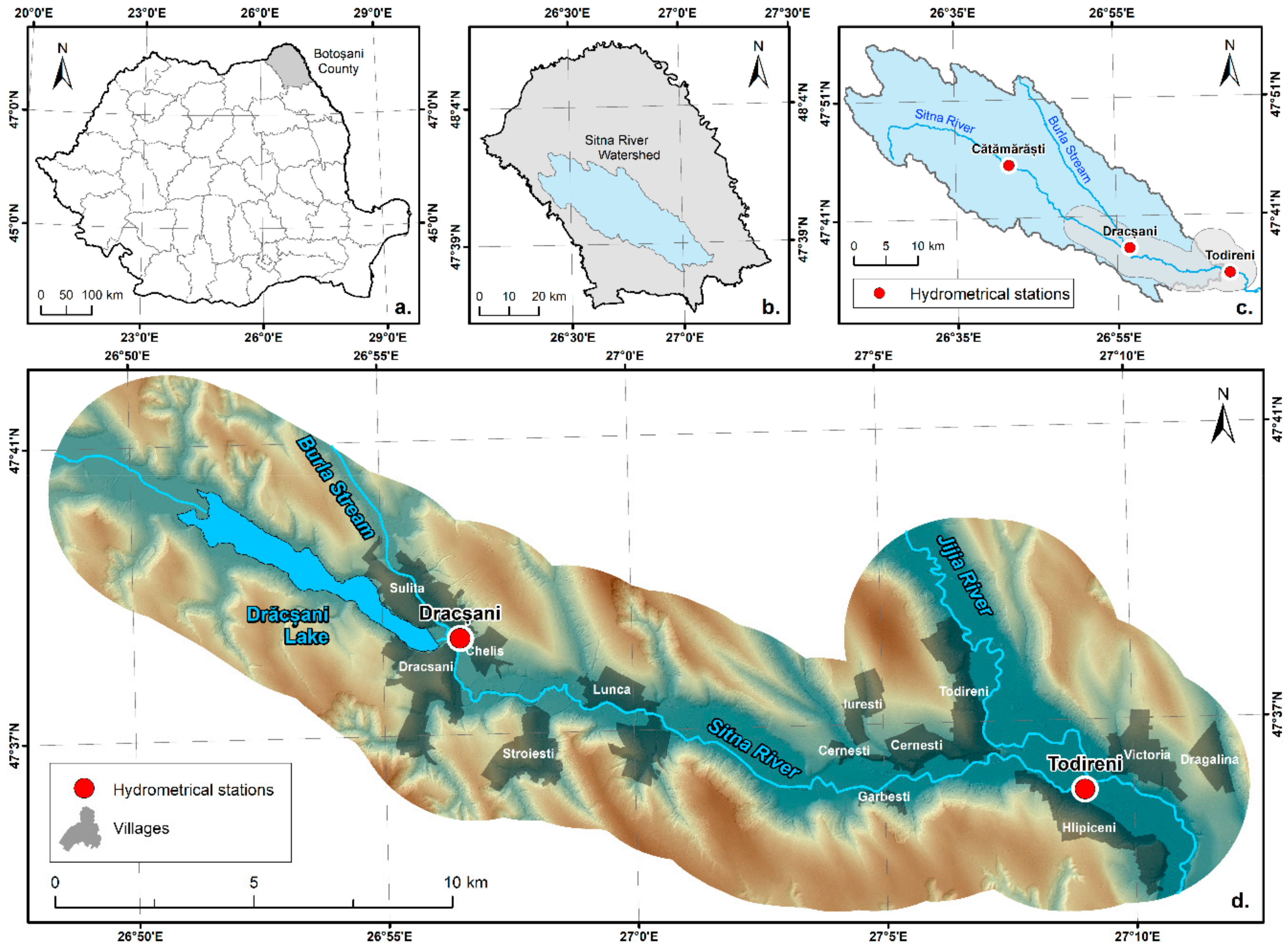
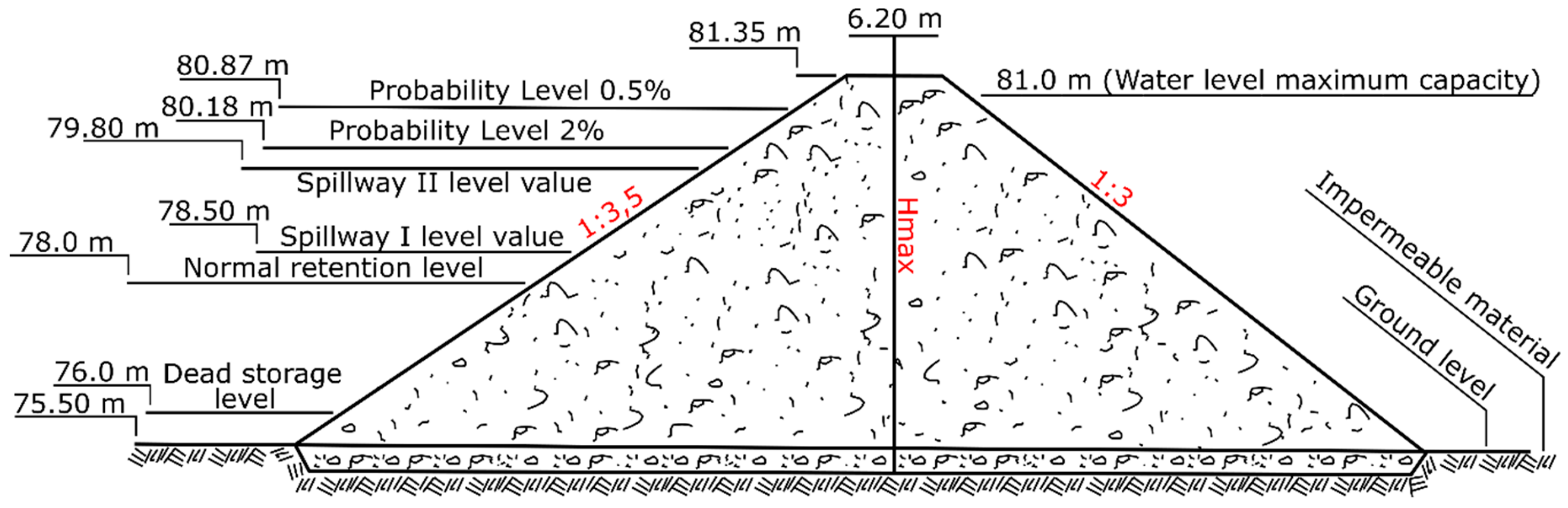
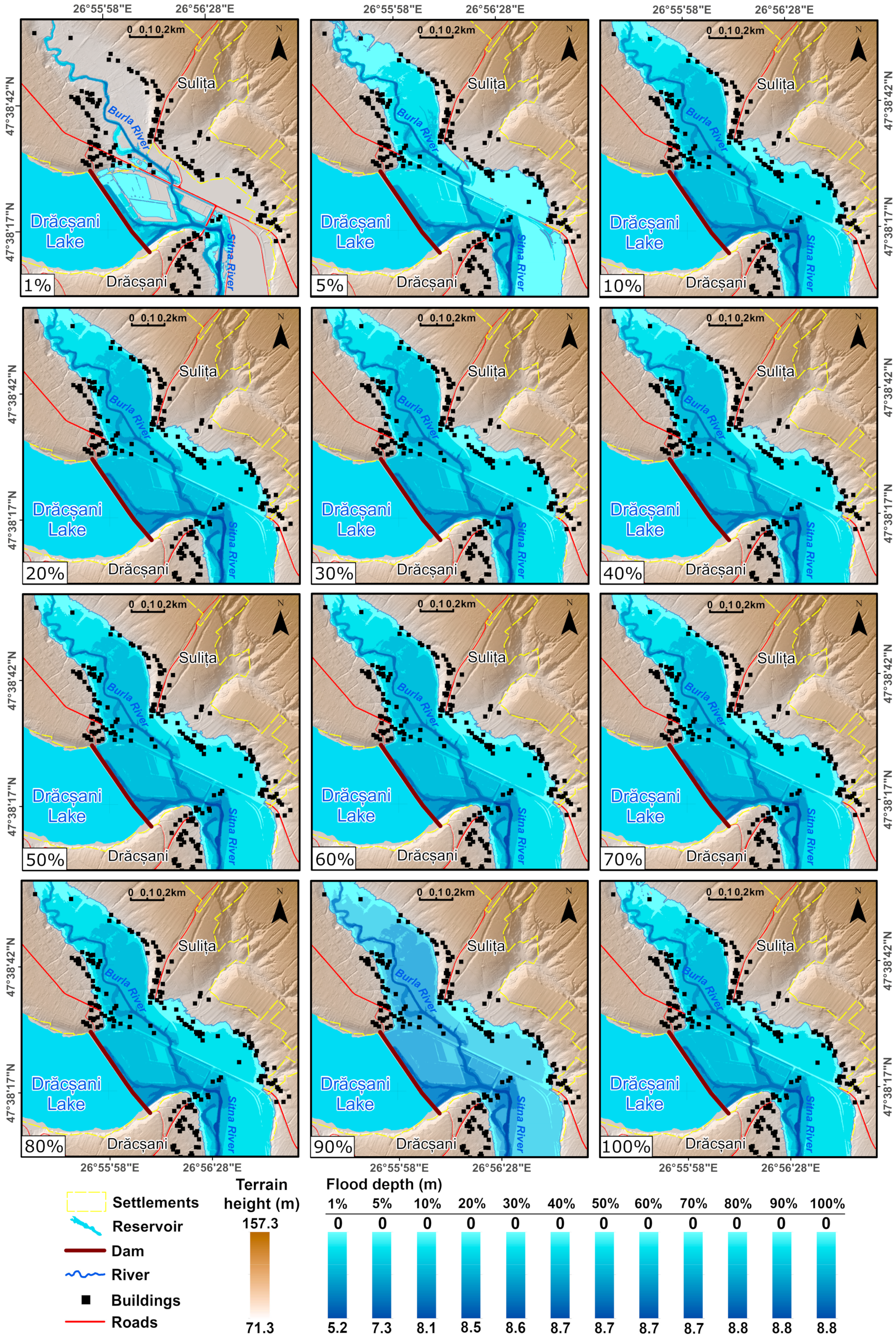
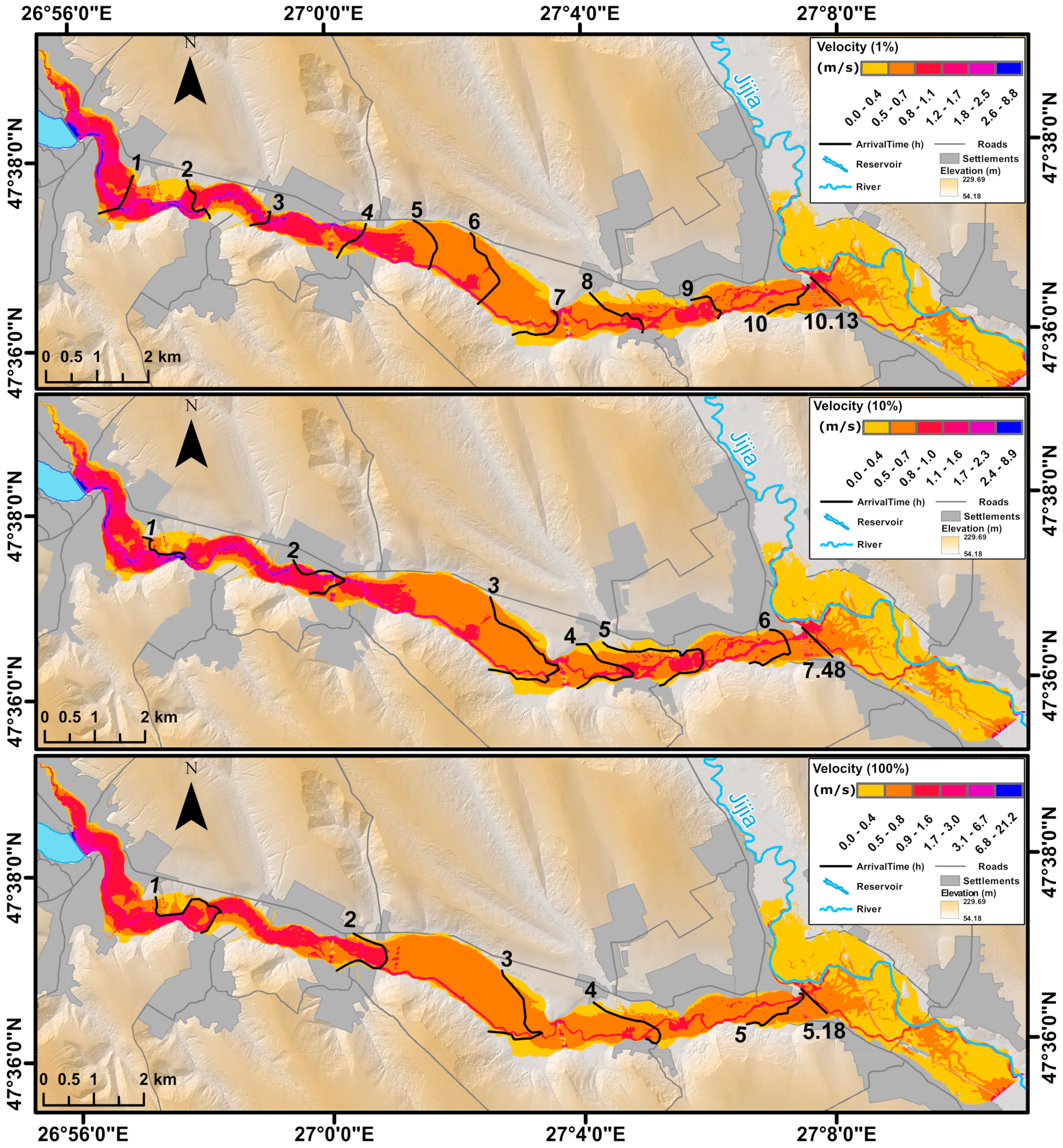
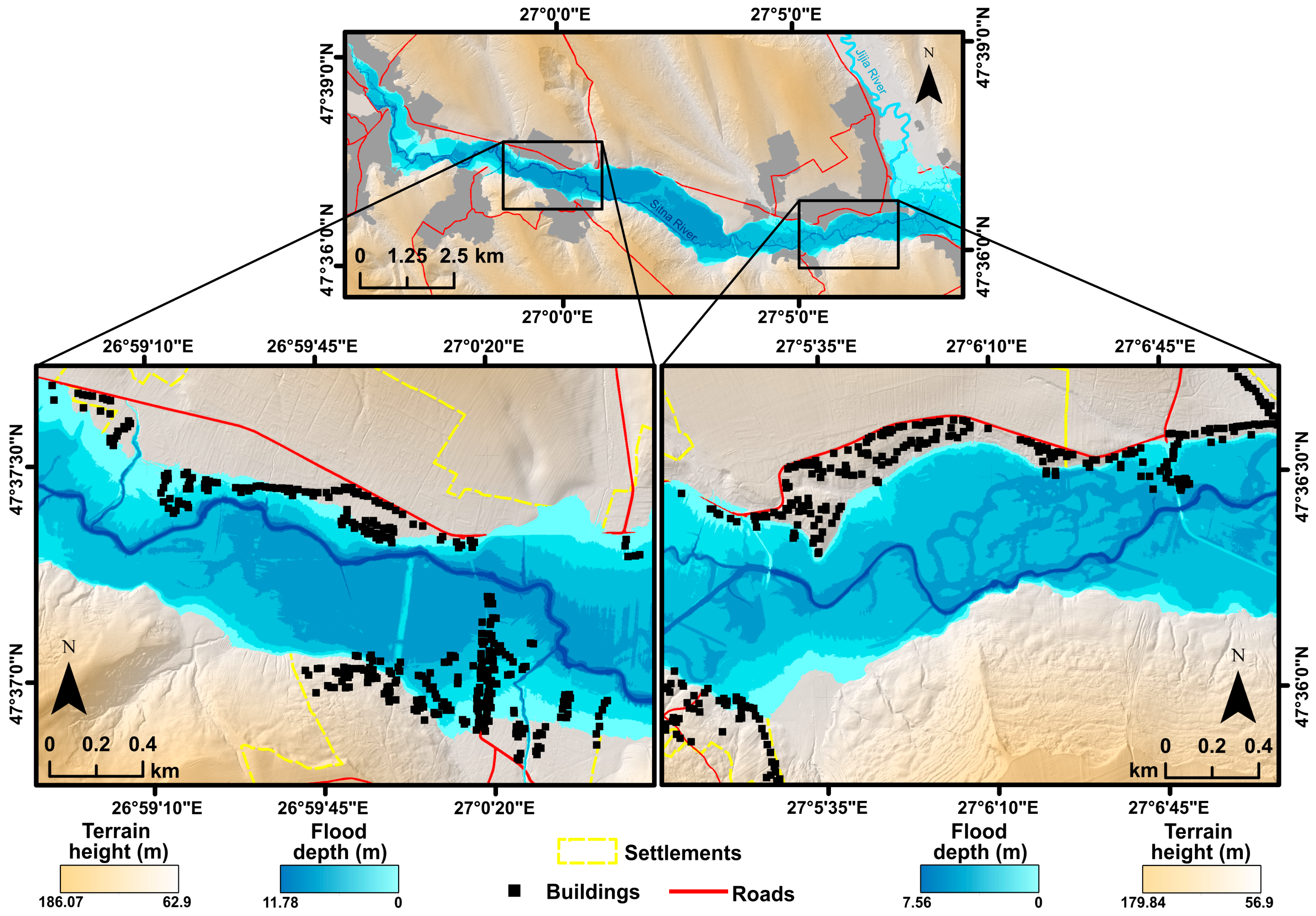
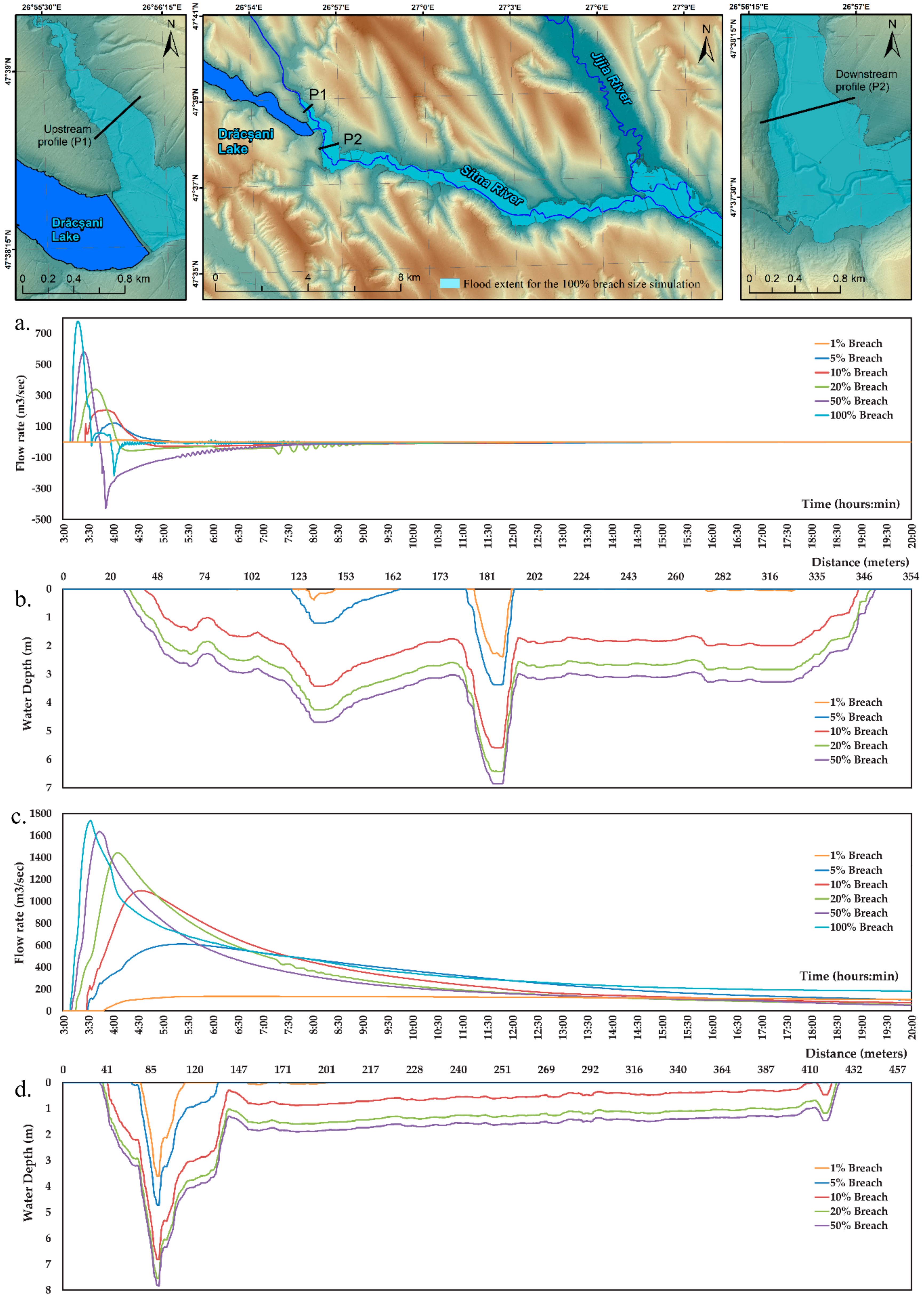
Table 1.
Morphometric parameters for Sitna river basin.
| Relief Ratio | Drainage Density | Form Factor | Circularity Ratio | Elongation Ratio |
|---|---|---|---|---|
| 5.28 | 1.31 | 0.21 | 0.14 | 0.52 |
Table 2.
Parameter comparison results for the given flood simulations, corresponding to each breach size.
Table 2.
Parameter comparison results for the given flood simulations, corresponding to each breach size.
| Breach Size | NFB | TFA (ha) | MWD (m) | MWV (m/s) | FPT(h) | RET (min) | AWV (m/s) |
|---|---|---|---|---|---|---|---|
| 1% | 36 | 1179.70 | 8.44 | 8.78 | 10 h 13 min | 54 h | 0.35 |
| 5% | 214 | 1876.74 | 9.95 | 8.80 | 7 h 59 min | 32 h | 0.57 |
| 10% | 233 | 1903.52 | 9.97 | 8.82 | 7 h 48 min | 23 h | 0.59 |
| 20% | 235 | 1908.71 | 10.01 | 8.83 | 5 h 41 min | 20 h | 0.60 |
| 30% | 238 | 1909.71 | 10.02 | 8.84 | 5 h 37 min | 14 h | 0.62 |
| 40% | 240 | 1913.38 | 10.05 | 9.19 | 5 h 32 min | 11 h | 0.62 |
| 50% | 241 | 1918.36 | 10.06 | 9.28 | 5 h 26 min | 8 h 15 min | 0.63 |
| 60% | 241 | 1921.03 | 10.07 | 10.13 | 5 h 21 min | 7 h 15 min | 0.63 |
| 70% | 242 | 1922.40 | 10.07 | 11.65 | 5 h 20 min | 6 h 30 min | 0.63 |
| 80% | 242 | 1926.84 | 10.08 | 12.91 | 5 h 19 min | 5 h 30 min | 0.63 |
| 90% | 242 | 1929.75 | 10.10 | 13.55 | 5 h 19 min | 4 h 15 min | 0.63 |
| 100% | 376 | 2068.34 | 11.76 | 21.78 | 5 h 18 min | 3 h 15 min | 0.68 |
NFB—Number of flooded buildings; TFA—Total flooded area; MWD—Maximum water depth; MWV—Maximum water velocity; FPT—Flood propagation time; RET—Reservoir evacuation time; AWV—Average water velocity.
Table 3.
Flooded areas, by land use category, according to Corine Land Cover 2018, for all breach sizes.
Table 3.
Flooded areas, by land use category, according to Corine Land Cover 2018, for all breach sizes.
| CLC Code | Flooded Areas (ha) | |||||||||||
|---|---|---|---|---|---|---|---|---|---|---|---|---|
| 1% | 5% | 10% | 20% | 30% | 40% | 50% | 60% | 70% | 80% | 90% | 100% | |
| 112 1 | 40.3 | 85.8 | 87.2 | 86.3 | 87.7 | 82.9 | 85.3 | 86.9 | 87.2 | 87.1 | 86.4 | 110.6 |
| 211 2 | 204.7 | 339.8 | 343.9 | 340.5 | 347.1 | 329.0 | 337.6 | 343.1 | 344.4 | 343.9 | 341.6 | 398.7 |
| 221 3 | - | 0.3 | 0.3 | 0.3 | 0.3 | 0.3 | 0.3 | 0.3 | 0.3 | 0.3 | 0.3 | 0.3 |
| 222 4 | 3.6 | 5.3 | 5.3 | 5.3 | 5.3 | 5.3 | 5.3 | 5.3 | 5.3 | 5.3 | 5.3 | 6.5 |
| 231 5 | 771.1 | 1095.8 | 1106.3 | 1094.0 | 1107.0 | 1092.1 | 1093.3 | 1099.0 | 1101.4 | 1100.6 | 1096.7 | 1163.3 |
| 242 6 | 25.5 | 108.1 | 110.0 | 109.4 | 107.7 | 94.7 | 108.4 | 109.6 | 109.4 | 109.5 | 109.0 | 105.8 |
| 243 7 | 117.3 | 164.5 | 164.6 | 164.7 | 165.3 | 164.8 | 164.2 | 164.9 | 165.0 | 165.0 | 164.8 | 173.2 |
1 Discontinuous urban fabric; 2 Non-irrigated arable land; 3 Vineyards; 4 Fruit trees and berry plantations; 5 Pastures; 6 Complex cultivation patterns; 7 Land principally occupied by agriculture, with significant areas of natural vegetation.
Table 4.
Flood extent area correlation.
| Study Results (10% Breach Size) | 2D Unsteady (10% Breach Flow Rate) | Correlation | |
|---|---|---|---|
| Area (m2) | 20,683,352.5 | 20,403,841.6 | 98.70% |
| Official 0.1% flood extent | 2D Unsteady flow—0.1% recurrence | Correlation | |
| Area (m2) | 9,466,001.6 | 8,537,745.3 | 90.20% |
| Study results (50% breach size) | Full momentum (50% breach size) | Correlation | |
| Area (m2) | 19,183,623.66 | 17,987,918.28 | 93.80% |
© 2020 by the authors. Licensee MDPI, Basel, Switzerland. This article is an open access article distributed under the terms and conditions of the Creative Commons Attribution (CC BY) license (http://creativecommons.org/licenses/by/4.0/).
Share and Cite
MDPI and ACS Style
Albu, L.-M.; Enea, A.; Iosub, M.; Breabăn, I.-G. Dam Breach Size Comparison for Flood Simulations. A HEC-RAS Based, GIS Approach for Drăcșani Lake, Sitna River, Romania. Water 2020, 12, 1090. https://doi.org/10.3390/w12041090
AMA Style
Albu L-M, Enea A, Iosub M, Breabăn I-G. Dam Breach Size Comparison for Flood Simulations. A HEC-RAS Based, GIS Approach for Drăcșani Lake, Sitna River, Romania. Water. 2020; 12(4):1090. https://doi.org/10.3390/w12041090
Chicago/Turabian StyleAlbu, Liviu-Marian, Andrei Enea, Marina Iosub, and Iuliana-Gabriela Breabăn. 2020. "Dam Breach Size Comparison for Flood Simulations. A HEC-RAS Based, GIS Approach for Drăcșani Lake, Sitna River, Romania" Water 12, no. 4: 1090. https://doi.org/10.3390/w12041090
Note that from the first issue of 2016, this journal uses article numbers instead of page numbers. See further details here.